BaSAL: Size Balanced Warm Start Active Learning for LiDAR Semantic Segmentation

Abstract

Active learning strives to reduce the need for costly data annotation, by repeatedly querying an annotator to label the most informative samples from a pool of unlabeled data and retraining a model from these samples. We identify two problems with existing active learning methods for LiDAR semantic segmentation. First, they ignore the severe class imbalance inherent in LiDAR semantic segmentation datasets. Second, to bootstrap the active learning loop, they train their initial model from randomly selected data samples, which leads to low performance and is referred to as the cold start problem. To address these problems we propose BaSAL, a size-balanced warm start active learning model, based on the observation that each object class has a characteristic size. By sampling object clusters according to their size, we can thus create a size-balanced dataset that is also more class-balanced. Furthermore, in contrast to existing information measures like entropy or CoreSet, size-based sampling does not require an already trained model and thus can be used to address the cold start problem. Results show that we are able to improve the performance of the initial model by a large margin. Combining size-balanced sampling and warm start with established information measures, our approach achieves a comparable performance to training on the entire SemanticKITTI dataset, despite using only 5% of the annotations, which outperforms existing active learning methods. We also match the existing state-of-the-art in active learning on nuScenes. Our code will be made available upon paper acceptance.

I Introduction

Autonomous vehicles are often equipped with LiDAR, a time-of-flight sensor that accurately scans the environment and excels at 3D perception tasks. Semantic segmentation is a popular task for LiDAR-based perception systems whose goal is to assign a predefined class label for each point in the LiDAR scan. Existing methods on this task are mostly learning-based and evaluated on large-scale benchmark datasets like SemanticKITTI [1] and nuScenes [2]. However, training such models requires a large amount of data, which is expensive to label. Active learning is a machine learning technique that reduces the demand for annotation by interactively selecting informative samples and querying an oracle for annotation [3].

Research on active learning for LiDAR (semantic) segmentation [4, 5] focuses on novel information measures that quantify the importance of unlabeled data, such that a limited annotation budget is spent on the most informative samples. We identify two problems that have not been explicitly addressed in existing active learning methods for LiDAR segmentation: class imbalance and the cold start problem.

The performance on the LiDAR segmentation task is commonly measured using the mean Intersection over Union (mIoU) metric, which assigns the same weight to all classes. However, since there is a strong class imbalance, models are trained on fewer points of rare classes, thus yielding a lower performance in general. Consequently, points belonging to rare classes have a larger impact on the mIoU metric. In contrast, the active learning budget is measured by the number of points, which treats points of all classes the same. This reveals a fundamental mismatch between the performance metric and the active learning budget. By reducing class imbalance in the sampled data, we can reduce this mismatch.

One approach to address class imbalance is to use a model trained on a small subset of labels to classify the unlabeled pool and pick samples according to their predicted label. In preliminary studies we found that this approach does not work well, as a weak model trained on a small amount of data is not able to detect rare classes and thus the approach breaks down. We find that objects sharing the same labels tend to be of similar sizes. Thus by creating a size-balanced dataset, we can also create a more class-balanced dataset.

The cold start problem [6] in active learning is about selecting an initial set of data for label acquisition and model training. Existing methods initialize the active learning loop by annotating randomly sampled data from a pool of unlabeled data [5, 4] and training a model with this data. They then compute their proposed information measure based on the outputs of the trained model to select the most informative samples. However, the performance of the initial model is often lacking, which affects subsequent active learning iterations. We then find that sampling objects according to their size does not require a trained model and can thus already be utilized in the first active learning cycle. Therefore such a method can address the cold start problem.

Following the above intuitions, we propose BaSAL, a size-balanced warm start active learning strategy that addresses the class imbalance and the cold start problem. To handle class imbalance, we propose Average Point Information (API), a metric that measures the informativeness of each object cluster using its size. We use the API metric to create partitions of clusters that have approximately the same amount of information. By sampling data from these partitions, our size-balanced sampling is also more class-balanced. To initiate model training, we uniformly sample clusters from all size partitions for label acquisition. For subsequent rounds of active learning, we adopt well-established information measures, such as entropy [7] and CoreSet [8] to rank unlabeled data and select top-ranking clusters from each partition for further label acquisition. Experiments on SemanticKITTI [1] show that by labeling only $5\%$ points, we are able to achieve a comparable performance of fully supervised learning. We also outperform existing active learning methods by a large margin on SemanticKITTI [1]. On nuScenes [2], our model performs competitively with the state-of-the-art LiDAL [5] method and reaches $95\%$ performance of fully supervised learning.

In summary, our contribution can be outlined as follows:

• Based on the insight that is non-trivial to sample objects according to their class, we instead propose a method that addresses class imbalance by sampling object clusters according to their size.

• We initialize our model by sampling data uniformly from the size-based partitions and thus address the cold start problem.

• Our experiments demonstrate that BaSAL outperforms the state-of-the-art in active learning on SemanticKITTI [1] and matches it on nuScenes [2].

II Related work

In this section we discuss the literature on active learning, class imbalance and the cold start problem in active learning. We focus on pool-based active learning that assumes a large pool of unlabeled data available [3].

II-A Active Learning

There are numerous strategies to query a new sample for label acquisition, including uncertainty-based methods, diversity-based methods or combinations of multiple approaches. Uncertainty-based methods select hard examples by measuring model disagreement [9, 10], entropy [7, 11], predicted loss [12], discriminator scores [13], or geometric distances to the decision boundary [14]. However, uncertainty-based methods tend to draw similar samples without taking diversity into account. Other works [8, 15, 16, 17] propose a diversity-based strategy that finds a subset of samples that best represents the entire pool. Follow-up works [18, 19] combine model uncertainty and diversity.

Recent research on active learning for LiDAR segmentation takes similar strategies, but exploits task-specific prior knowledge. LiDAL [5] considers inconsistencies in model predictions across frames as the uncertainty measure for informative sample selection. ReDAL [4] divides a point cloud into regions and then selects diverse regions according to multiple cues, including softmax entropy, color discontinuity, and structural complexity. [20] proposes a diversity-based method for 3D object detection by enforcing both spatial diversity and temporal diversity. [21] uses detection and prediction entropy as the information measures for the prediction and planning tasks. Similar to previous works [5, 4], we take both uncertainty and diversity as our information measure.

II-B Class imbalance problem in active learning

Class imbalance is a common problem for datasets collected in the wild.  [22] summarizes two kinds of techniques to cope with the class imbalance problem: Density-sensitive active learning and skew-specialized active learning [23]. The former assigns an informativeness score to each sample by imposing an assumption on the input space. Examples include information density [24], pre-clustering [25] and alternate density-sensitive heuristics [26]. The latter incorporates a bias towards underrepresented classes, thus resulting in a more balanced sampling [27, 28, 29]. [30] addresses class imbalance in active learning for visual tasks by introducing a sample balancing step that prioritizes minority classes. However, most methods require a pretrained model. In contrast, we tackle class imbalance in LiDAR segmentation without pretraining by creating size-balanced partitions as size is a characteristic trait of class.

II-C Cold start in active learning

Cold start in active learning refers to the problem of which data to label first given an unlabeled pool of data [6]. The labeled data is then used to train an initial model which serves as the starting point of active learning. [31, 32] take advantage of pre-trained models and cluster unlabeled samples in the embedding space. Those samples closer to the cluster centers are selected for annotation, as they better represent categories than random samples. [33] focuses primarily on selecting examples that are hard to learn via self-supervised contrastive learning, based on the assumption that if a model can not separate a sample from others, this sample is expected to exhibit typical characteristics, such as common visual patterns in vision, that are shared by others. [34] proposes TypiClust that aims to find out typical examples which better represent the entire dataset. The typicality of a sample is measured by the inverse of the average Euclidean distance to its K-nearest neighbors in the feature space. [35] proposes ProbCover, a solution for cold start that maximizes the probability of covering the unlabeled set in the embedding space. [6] uses pseudo labels to pre-train models and then rank unlabeled data by uncertainty, after which the top-ranking samples are used for label acquisition. We handle the cold start problem by a simple size-based sampling.

III Method

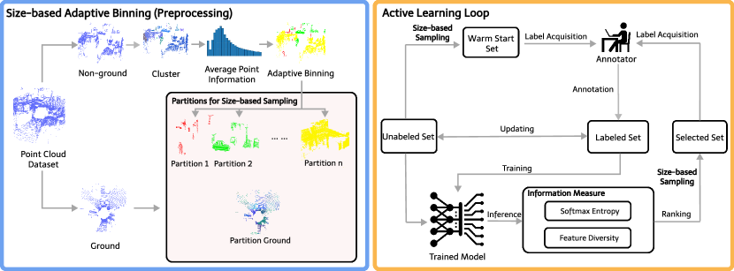
Figure 1: Overview of BaSAL. Our framework consists of a preprocessing step and the active learning loop. Size-balanced sampling is used both to determine the warm start set, as well as the selected set for successive active learning iterations.

Fig. 1 shows an overview of BaSAL, which consists of a preprocessing step and the active learning loop. We preprocess the input point clouds to create multiple partitions for size-balanced sampling (Section III-A). During the active learning loop, we use size-based sampling (Section III-B) in both the model initialization phase (warm start) and subsequent active learning iterations to ensure a size-balanced training set. After warm starting the model, we adopt popular information measures (Section III-C) to rank and select the most informative clusters from each partition, until we exceed the annotation budget. Then we add them to the labeled set and retrain the model.

III-A Size-based Adaptive Binning

Given a dataset $\mathcal{D}$, we first apply ground plane detection and obtain the ground points which are further split into a number of grids $\mathcal{G}$ of size 10m $\times$ 10m. The remaining non-ground points are split into a collection of class-agnostic clusters $\mathcal{C}$ using HDBSCAN [36]. Based on the assumption that objects of similar sizes tend to share the same semantic labels, we group the class-agnostic clusters $\mathcal{C}$ by size, i.e. the sum of the dimensions of the 3D bounding box that encloses a cluster. We round all sizes to integers. To balance the information among sizes, we calculate the Average Point Information (API) per size, by

$$API_{s}=\left(\frac{logP_{s}}{C_{s}}\right)^{-1},$$ (1)

where $C_{s}$ is the number of clusters and $P_{s}$ is the number of accumulated points from all clusters, for a particular size $s$. $\frac{P_{s}}{C_{s}}$ stands for the average number of points per cluster and the additional logarithm penalizes larger clusters, as each additional point brings less information gain. We adaptively bin all sizes by API and obtain several partitions such that the accumulated API inside each partition is approximately the same. We show an example in Fig. 2, where the number of partitions $B$ is set to 3.

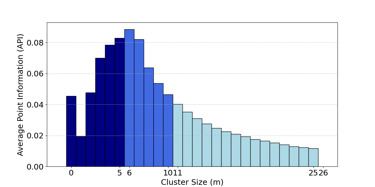
Figure 2: Adaptive binning over sizes. We split all size groups into 3 partitions, as indicated by colors. The accumulated API from each partition is approximately the same. We balance object classes by creating a size-based partition.

III-B Size-based Sampling

We employ size-based sampling in two places in our pipeline. In the initial active learning iteration, most works [4, 5] use random sampling. Instead we sample clusters uniformly from all partitions (including the ground partition). This achieves the desired warm start. In later active learning iterations, most works [4, 5] rank samples according to one or several information criteria and select the top-ranking samples. Instead we rank clusters within each size-based partition using standard information measures (Section III-C).

III-C Information measures

To rank clusters, we combine two well-established information measures: Softmax entropy [7] and feature diversity (CoreSet) [8]. Entropy aims to select the data that the model is most uncertain of. Feature diversity (CoreSet) prioritizes unlabeled data that is far from the labeled data in the latent space to ensure diversity. After ranking, we choose the top-ranking clusters for training a network that will be used in the next active learning iteration.

III-C1 Softmax entropy

We calculate the entropy for each unlabeled cluster, where $N$ is the number of points in a cluster and $p$ is the predicted probability per point:

$$E=-\frac{1}{N}\sum_{n=1}^{N}p_{n}\log(p_{n})$$ (2)

III-C2 Feature diversity

We use the feature from the last layer in the encoder-decoder network before classification and calculate the mean feature vector f for each cluster. The feature diversity $D_{j}$ is defined as the summed Euclidean distance between an unlabeled cluster $j$ and all $N_{l}$ labeled clusters from the same partition:

$$D_{j} =\sum_{i=1}^{N_{l}}||\textbf{f}_{i}-\textbf{f}_{j}||_{2}$$ (3)

III-C3 Combination

We sort all unlabeled clusters by entropy and diversity per partition, as defined Eq. (4), where $r_{j}^{E}$ and $r_{j}^{D}$ denote the rank for $j$ th cluster in terms of entropy and diversity, respectively. $\mathcal{D}_{u}^{b}$ indicates the collection of unlabeled clusters from partition $b$.

$$r_{j}=\underset{j\in\mathcal{D}_{u}^{b}}{argsort}\left(\frac{1}{r_{j}^{E}}+\frac{1}{r_{j}^{D}}\right)$$ (4)

IV Experiments

We conduct extensive experiments on SemanticKITTI [37] and nuScenes [2] datasets, and compare with baselines [5, 4] on LiDAR segmentation task.

IV-A Datasets and Evaluation Metric

On SemanticKITTI, we take sequences $00-07$ and seq $09-10$ for training and report the performance on validation sequence $08$. On nuScenes, we train our model on the official training split which contains 700 scenes, and report the performance on the validation split with 150 scenes. We compare the mean Intersection over Union (mIoU) metric. There are 19 semantic classes on SemanticKITTI and 16 classes on nuScenes, respectively.

IV-B Experimental settings

IV-B1 Network Architectures

Following ReDAL [4] and LiDAL [5], we test our model with two backbone architectures: SPVCNN [38] based on point-voxel CNN, and MinkowskiNet [39] based on sparse convolution.

IV-B2 Baselines

We select nine baselines for comparison, including random point cloud selection (RAND), softmax confidence (CONF) [40], softmax margin (MAR) [40], softmax entropy (ENT) [40], MC-dropout (MCDR) [41], CoreSet selection (CSET) [8], segment-entropy (SEGENT) [42], ReDAL [4] and LiDAL [5]. Experimental results come from from LiDAL [5].

IV-B3 Active Learning Protocol

BaSAL training has two stages: warm start initialization and subsequent active learning. We warm start the model by size-based sampling. The annotation budget in this phase is $x_{init}\%$. After warm start, we conduct $K$ active learning iterations. During each iteration, we interactively select top-ranking clusters from each partition for label acquisition such that the total annotation is no greater than $x_{active}\%$, We load the previous checkpoint and fine-tune the model with all labeled data.

The labeling budget is measured as the percentage of the labeled points with respect to the entire dataset. For both SemanticKITTI [1] and nuScenes [2], we set $x_{init}=1$, $K=4$, and $x_{active}=1$. The annotation budget is uniformly distributed over all partitions and the ground grid in each active learning iteration. We report the average result over three runs.

IV-C Main Results

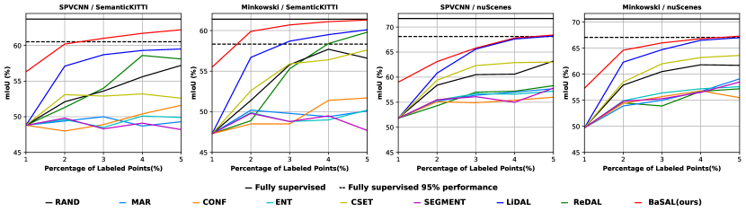
Figure 3: Experiment results of different active learning strategies on SemanticKITTI [1], nuScenes [2] using SPVCNN [38], Minkowski [39] network. We compare BaSAL with other existing works. The solid line is the performance of the fully supervised model. The dashed line indicates 95% performance of the fully supervised model. Our model outperforms all existing active learning approaches on SemanticKITTI and gets on par performance with the state-of-the-art active learning method LiDAL [5] on nuScenes.

Fig. 3 compares BaSAL with all baselines. The x-axis represents the percentage of labeled points with respect to the entire training set and the y-axis represents performance (mIoU). On SemanticKITTI, our model consistently outperforms all baselines in all settings. When the annotation budget increases to $5\%$, BaSAL (with Minkowski backbone) is able to match the performance of fully supervised training on the entire dataset, demonstrating the benefit of active learning in reducing annotation effort. BaSAL with the SPVCNN backbone still achieves 98$\%$ the performance of the fully supervised model. On the nuScenes dataset, BaSAL surpasses all the baselines given $1\%$, $2\%$ and $3\%$ labeled data. LiDAL[5] is able to match the performance of BaSAL when the annotation budget is up to $5\%$. Both models reach $95\%$ performance of fully supervised learning. We also compare the performance between cold and warm start at $1\%$. Notably, the advantage of our model over other baselines is more than $5\%$ mIoU on both datasets, validating the advantage of our warm start in tackling the cold start problem.

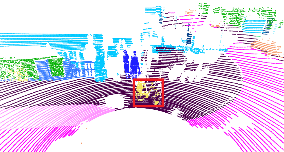
(a) Ground Truth

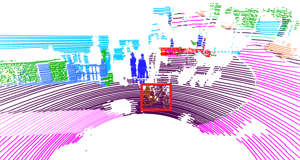
(b) Fully Supervised (100%)

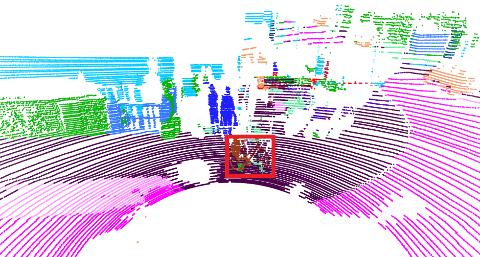
(c) ReDAL (5%)

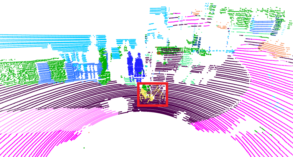
(d) BaSAL (5%)

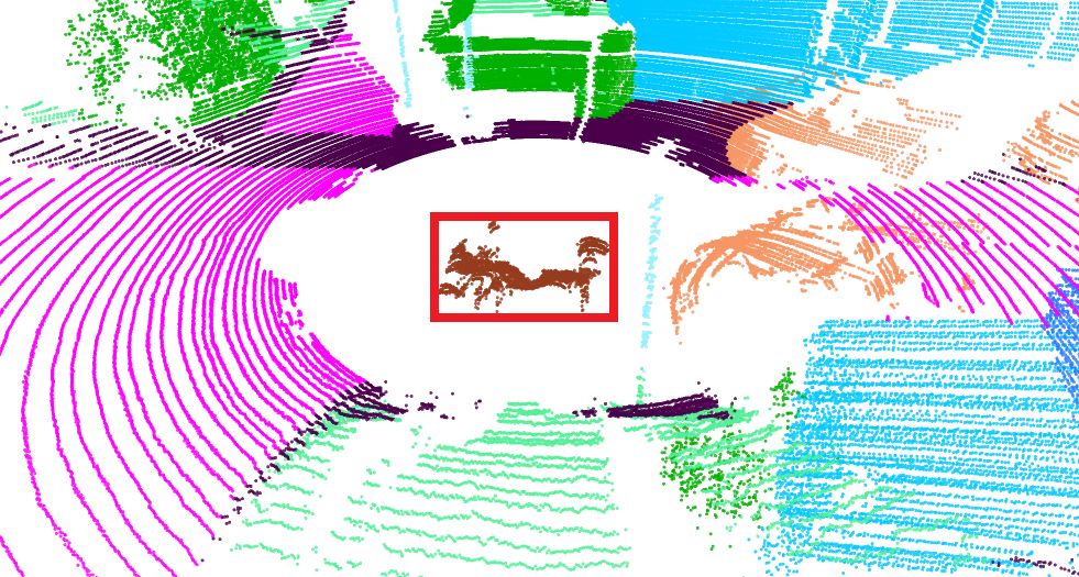
(e) Ground Truth

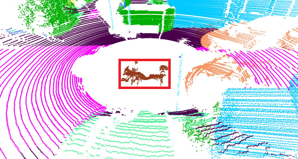
(f) Fully Supervised (100%)

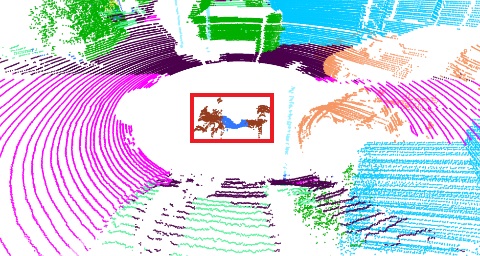
(g) ReDAL (5%)

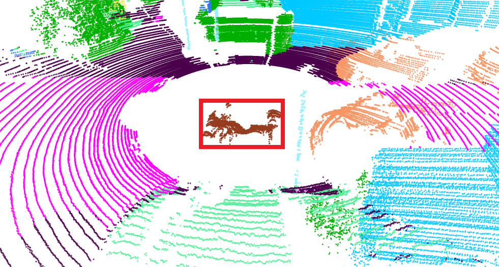
(h) BaSAL (5%)

Figure 4: Qualitative comparison on SemanticKITTI [1] using the Minkowski [39] backbone. We visualize semantic segmentation results on two examples. Our model successfully detects the bicycle in (d), as indicated by the red box. In comparison, other models misclassify the bicycle as sidewalks in (b) and (c). In the second example, our model better detects the motorcycle in (h), while ReDAL [4] over-segments the motorcycle. We improve the performance on underrepresented classes.

TABLE I: Class distribution on SemanticKITTI [1]. We calculate the class distribution over the entire dataset and over partitions of different size. We use 3 partitions and ground. Classes are highly imbalanced over the dataset and we can observe that most classes have a characteristic size (highlighted in bold text).

	car	bicycle	motorcycle	truck	other vehicle	person	bicyclist	motorcyclist	road	parking	sidewalk	other ground	building	fence	vegetation	trunk	terrain	pole	traffic sign
Entire dataset	5.7	0.01	0.05	0.3	0.3	0.04	0.02	0.005	27.3	2.0	19.7	0.5	10.2	3.9	18.6	0.8	10.3	0.3	0.07
Partition1 (small)	26.7	23.4	77.3	3.6	17.7	53.9	68.2	76.3	0.1	0.1	0.2	1.2	6.5	4.4	9.3	48.7	1.1	42.9	50.5
Partition2 (medium)	63.9	14.3	10.6	29.6	56.5	23.2	24.3	18.1	0.1	0.2	0.2	1.6	13.1	9.0	18.0	33.2	1.7	19.6	23.6
Partition3 (large)	6.5	40.4	6.9	62.9	23.7	17.8	5.6	0.8	0.1	0.1	0.4	4.4	71.1	49.8	50.7	14.7	3.4	31.6	25.7
Ground Partition	2.8	21.9	5.2	3.9	2.1	5.1	1.9	4.9	99.7	99.6	99.3	92.7	9.3	36.8	22.1	3.5	93.9	5.8	0.2

TABLE II: Performance on less frequent classes. We measure mIoU (%) on SemanticKITTI [1] using the Minkowski [39] backbone. We also calculate the proportion of points per class with respect to the full dataset. Our model boosts the performance on rare classes substantially, verifying the advantage of our model in tackling class imbalance. FS stands for fully supervised learning on the full dataset.

	bicycle	motorcycle	person	bicyclist	motorcyclist
$\%$	0.01	0.05	0.04	0.02	0.005
RAND	9.5	45.0	52.0	47.8	0.0
ReDAL	29.6	58.6	63.4	84.1	0.5
FS	20.4	63.9	65.0	78.5	0.4
Ours	43.5	70.6	70.4	88.4	0.2

IV-D Ablation study

TABLE III: Ablation study. We conduct our ablation on SemanticKITTI [1]. We train all models from scratch in iteration 1 and fine-tune them in iteration 2-5. Our size-based partition contributes the most to the final performance. RS: random sampling from all unlabeled data; SS: size-based sampling; EN: softmax entropy as the information measure; FD: feature diversity as the information measure [8].

Iteration 1	Iteration 2-5				mIoU(%)
Initialization	Info measure		Data Sampling
	EN	FD	RS	SS
Cold start			✓		56.8
				✓	60.1
Warm start				✓	60.4
	✓			✓	61.1
	✓	✓		✓	61.3

IV-D1 Method ablation

We numerically evaluate the contribution of each component in our design on SemanticKITTI [1] in Tab. III. RS stands for random sampling from all unlabeled clusters. SS represents size-based sampling. EN and FD indicate the information measures: entropy and feature diversity, respectively. We first ablate our size-based partition. Without relying on any learning-based information measures, our model gains a 3.3% improvement, by simply replacing the random sampling with our size-based partition, when using cold start. Notably, this is the most significant increase in our ablation study. Warm starting the model further results in a $0.3\%$ improvement. Next, we evaluate the effect of information measures. Adding softmax entropy as an information measure increases the result by $0.7\%$. Taking feature diversity as an extra measure marginally improves the result by $0.2\%$.

IV-D2 Number of partitions

We also experiment with different numbers of partitions when warm starting the model. We set the number of partitions $B$ to 3, 6, 12 and 25 partitions, and achieve 56.3%, 56.1%, 55.4% and 54.8% mIoU. In general, we find the number of partitions has a minor impact on the performance when $B$ is between 3 and 6. It is also worth mentioning that our approach avoids setting the size boundaries manually, as it determines the boundaries directly from the adaptive binning, thus reducing the number of hyperparameters.

IV-E Analysis of class imbalance

IV-E1 Analysis on less frequent classes

We show our results on less frequent classes in Tab. II. We outperform ReDAL and fully supervised learning by a substantial margin on four classes: bicycle, motorcycle, person and bicyclist. For example, the advantage over baselines is more than $20\%$ on the bicycle class and approximately $10\%$ on the bicyclist class. It is worth noting that these two classes only occupy $0.01\%$ and $0.02\%$ of the entire dataset. We attribute the remarkable improvement to our size-based partition which better handles class-balance. We show qualitative results on two samples in Fig. 4. In the top row, our model is able to recognize the bicycle, labeled by the red box in (d), while other models fail. In the second row, our model better segments the motorcycle than ReDAL [4], verifying our advantage in segmenting underrepresented classes.

IV-E2 Analysis on size-based partition

We also analyze the distribution of all classes on SemanticKITTI in Tab. I. We first enumerate the proportion of each class and then calculate the distribution of each class after size-based partition. All the numbers are vertically normalized by classes over partitions. One key observation is that each object class has a size bias, which aligns with our assumption that size is an informative cue to distinguish classes. For example, the less frequent classes, person, motorcyclist and motorcycle, come mostly from partition 1. Compared to random sampling from the entire dataset, sampling from partition 1 is likely to increase the chance of obtaining an underrepresented object class, thus reducing the class imbalance considerably. However, we also notice that the majority of the bicycle class falls in partition 3. We suspect that in the real world, bicycles have much fewer points. Consequently, they may not be well separated by HDBSCAN [36].

V Discussion

Active learning aims to reduce the labeling effort. However, recent works use different techniques to quantify labeling effort. [43] counts the number of frames and bounding boxes. ReDAL [4], LiDAL [5], Just Label What You Need [21] count the number of point labels. Some other works measure the number of clicks of an annotator, such as OneThingOneClick [44] and LESS [45]. LESS achieves approximately 100% performance using only 0.1% of the annotations. A crucial difference between our method and LESS is that they require the annotator to inspect the entire dataset, whereas in our case the annotator only inspects 5% of the data.

VI Conclusion

We present BaSAL, a size-based warm start strategy for active learning on LiDAR semantic segmentation. BaSAL reduces the class imbalance in large-scale autonomous driving datasets by sampling from a size-based partition. Our intuition is that each object class has a characteristic size. Thus we are able to indirectly reduce the class imbalance and the cold start problem by grouping class-agnostic clusters according to size. We fuse the size-based partition into state-of-the-art active learning models and improve the performance considerably. Particularly, on SemanticKITTI we achieve the same performance as fully supervised learning on the entire dataset, while using only $5\%$ of the annotation. Meanwhile, we boost the performance on less frequent classes significantly. Future work will explore better ways to create the object clusters, e.g. via a self-supervised learning-based approach. Furthermore, we want to develop a novel cost function to accurately quantify human annotation effort.

Supplementary Material

The supplementary material is organized as follows: Section A describes the implementation details. Section B visualizes the query units adopted in baselines and our work. Section C provides more details for the experimental results on SemanticKITTI [1] and nuScenes [2].

A. Implementation Details

A.1 Network Training

All experiments are conducted with a single A40 GPU. For SemanticKITTI [1], we set the training batch size to 10 and validation batch size to 20. We first train our network using the warm start data for 100 epochs. Then we finetune the model for 30 epochs for each active learning iteration. For nuScenes [2], we set the training batch size to 30 and validation batch size to 60. The warm start data is first trained for 200 epochs and then finetuned for 150 epochs for each active learning iteration. For both datasets, we train the networks by minimizing the cross-entropy loss using an Adam optimizer with an initial learning rate of 1e-3.

A.2 Size-based Adaptive Binning (Preprocessing)

We explain our size-based adaptive binning step in detail. Given a point cloud dataset, we first use PatchWork++ [46] with the default parameters to separate the ground points and the non-ground points. The ground points are then divided into grids of size 10m $\times$ 10m, named Partition Ground. For non-ground points, we use the HDBSCAN clustering  [36] algorithm to split them into clusters. In the algorithm, we set $min\_cluster$, $min\_samples$ and $cluster\_selection\_epsilon$ to be 20, 10 and 0.5 for SemanticKITTI and 20, 1 and 0.5 for nuScenes. We then calculate the size of all the non-ground clusters. The size of a cluster is defined by the rounded value of the sum of the length, width and height of its bounding box. We filter those clusters with a size larger than 25 meters. For clusters smaller than 25m, as mentioned in Section III-A, we calculate the Average Point Information (API) metric and adaptively group the sizes to 3 partitions to balance their information. The size ranges calculated by API are [0-5m, 6-10m, 11-25m] for SemanticKITTI and [0-7m, 8-12m, 13-25m] for nuScenes.

A.3 Size-based Sampling

The size-based sampling method is used in both the warm start step and successive active learning iterations. For warm start (1% budget), we uniformly sample clusters from Partition 1, Partition 2, Partition 3, and Partition Ground until the accumulated number of points of the clusters in each Partition reaches 0.25% of the entire dataset. For each successive active learning iteration, we increase the point budget by 1%, which is also uniformly allocated to the partitions mentioned above. Different from the sampling approach used in warm start, we uniformly select the top-ranking clusters from each partition after calculating the information measure, as mentioned in Section  III-C. The budget for each partition is also 0.25%, such that the total number of labeled points is 1% of the entire dataset.

B. Visual comparison of query units

Different active learning approaches query the oracle annotator to label samples at different levels of granularity, which we call query units. Common query units include entire point clouds [43, 21], supervoxels  [4, 5] or the more fine-grained object clusters used in our model. We qualitatively compare the supervoxels and object clusters in Fig. 5. ReDAL and LiDAL use the VCCS [47] algorithm to construct supervoxels. As shown in Fig. 5(b), the algorithm separates the point cloud frame to several connected supervoxels. However, compared with the ground truth object clusters, the supervoxels of the baselines are coarse, which often puts many different objects in one supervoxel (undersegmentation). In addition, the car at the bottom is segmented into two different supervoxels (oversegmentation). In contrast, as shown in Fig. 5(c), our clustering pipeline separates different objects well, making the querying and sampling process more fine-grained and accurate.

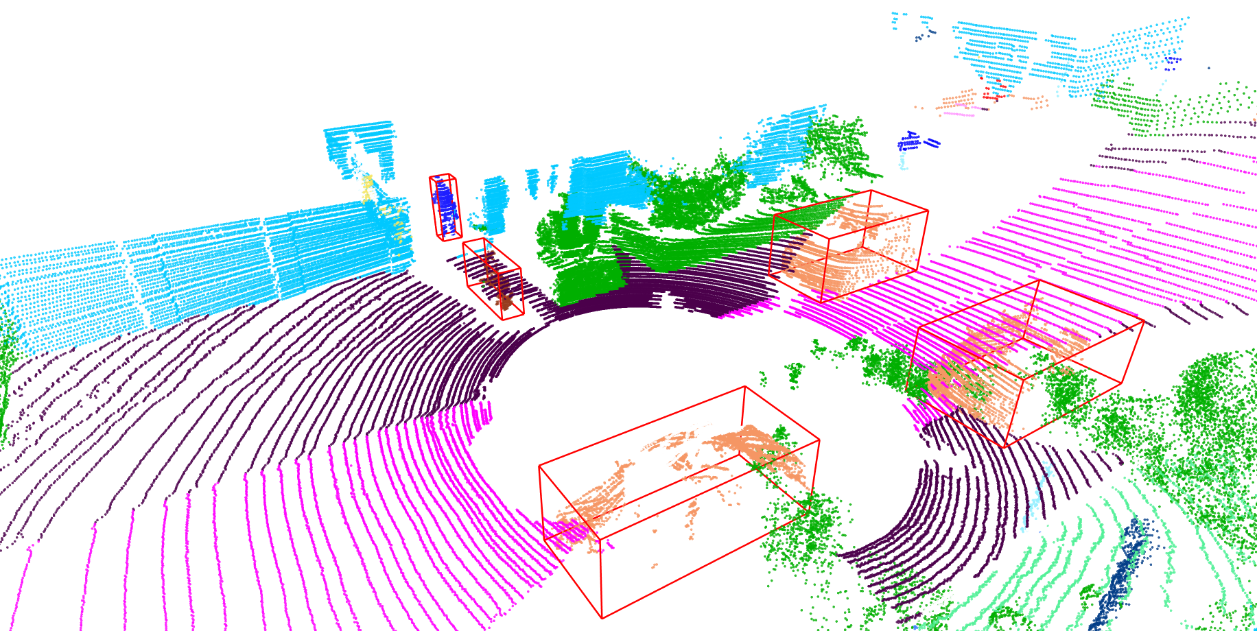
(a) Ground truth semantic labels.

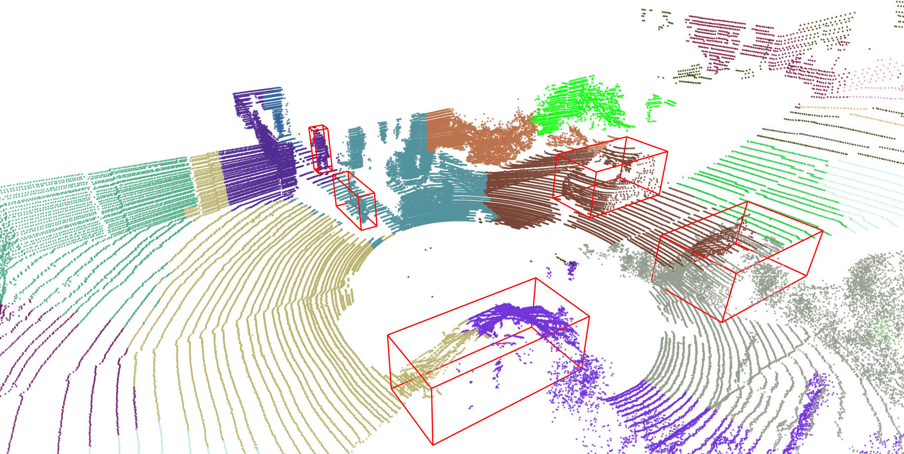
(b) Supervoxels used in ReDAL [4] and LiDAL [5].

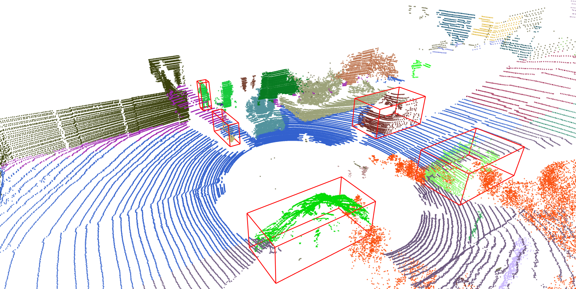
(c) Object clusters used in our work.

Figure 5: Visualization of the object clusters and the supervoxels. Points with the same color belong to one supervoxel (cluster). Red bounding boxes indicate ground truth object clusters.

C. Details on the Main Results

The baseline experiment results are taken from LiDAL [5], including random selection (RAND), softmax confidence (CONF), softmax margin (MAR), softmax entropy (ENT), MC-Dropout (MCDR), Core-Set selection (CSET), segment-entropy (SEGMENT), ReDAL, and LiDAL.

Tab. IV shows the numerical results (mIoU) on the SemanticKITTI [1] validation set with the SPVCNN [38] network, which aligns with Fig. 3. With 1% labeling budget, we achieve 56.3% mIoU, outperforming the baselines (48.8%) by a large margin. When the budget increases to 5%, we reach 62.2% mIoU, improving previous state-of-the-art by 2.7%.

Methods	Init 1%	2%	3%	4%	5%
RAND	48.8	52.1	53.6	55.6	57.2
MAR	48.8	49.4	50.0	48.7	49.3
CONF	48.8	48.0	48.9	50.4	51.6
ENT	48.8	49.6	48.5	50.1	49.9
CSET	48.8	53.1	52.9	53.2	52.6
SEGMENT	48.8	49.8	48.3	49.1	48.2
ReDAL	48.8	51.3	54.0	58.6	58.1
LiDAL	48.8	57.1	58.7	59.3	59.5
BaSAL (Ours)	56.3	60.2	61.0	61.7	62.2

TABLE IV: Mean intersection over union (%) on SemanticKITTI [1] validation set with SPVCNN [38] network.

Tab. V shows the mIoU results on SemanticKITTI [1] validation set with Minkowski [39] network. We achieve an 8.2% improvement over other baselines using 1% annotation budget. Given 5% annotation budget, we reach 61.3% mIoU, outperforming the previous state-of-the-art.

Methods	Init 1%	2%	3%	4%	5%
RAND	47.3	51.4	55.8	57.7	56.6
MAR	47.3	50.2	49.8	49.4	50.1
CONF	47.3	48.5	48.5	51.4	51.7
ENT	47.3	49.9	48.8	49.0	50.2
CSET	47.3	52.6	55.9	56.4	57.6
SEGMENT	47.3	49.8	48.8	49.5	47.7
ReDAL	47.3	56.7	58.7	59.5	60.1
LiDAL	47.3	51.4	55.8	57.7	56.6
BaSAL (Ours)	55.5	59.9	60.7	61.1	61.3

TABLE V: Mean intersection over union (%) on SemanticKITTI [1] validation set with Minkowski [39] network.

Tab. VI and Tab. VII show the mIoU results on the nuScenes [2] validation set with SPVCNN [38] and Minkowski [39] network, respectively. We substantially improve over the baselines by approximately 8% using 1% of the annotation budget. We also match the state-of-the-art for a budget of 5%.

Methods	Init 1%	2%	3%	4%	5%
RAND	51.8	58.4	60.5	60.6	63.2
MAR	51.8	55.2	56.4	57.0	57.7
CONF	51.8	55.1	54.9	55.4	56.0
ENT	51.8	55.4	56.7	56.6	57.2
CSET	51.8	59.4	62.3	62.9	63.0
SEGMENT	51.8	55.5	56.1	55.0	57.8
ReDAL	51.8	54.3	57.0	57.2	58.3
LiDAL	51.8	60.8	65.6	67.6	68.2
BaSAL (Ours)	59.0	63.1	65.8	67.8	68.4

TABLE VI: Mean intersection over union (%) on nuScenes [2] validation set with SPVCNN [38] network.

Methods	Init 1%	2%	3%	4%	5%
RAND	49.7	57.9	60.5	61.8	61.7
MAR	49.7	53.9	55.0	56.7	59.1
CONF	49.7	54.4	55.7	56.8	55.5
ENT	49.7	54.9	56.4	57.2	57.6
CSET	49.7	58.5	62.0	63.2	63.6
SEGMENT	49.7	54.8	55.3	56.5	58.5
ReDAL	49.7	54.5	53.9	56.7	57.2
LiDAL	49.7	62.3	64.7	66.5	67.0
BaSAL (Ours)	57.3	64.6	66.0	66.8	67.3

TABLE VII: Mean intersection over union (%) on nuScenes [2] validation set with Minkowski [39] network.

References

- [1] J. Behley, M. Garbade, A. Milioto, J. Quenzel, S. Behnke, C. Stachniss, and J. Gall, “Semantickitti: A dataset for semantic scene understanding of lidar sequences,” in ICCV, 2019, pp. 9297–9307.
- [2] H. Caesar, V. Bankiti, A. H. Lang, S. Vora, V. E. Liong, Q. Xu, A. Krishnan, Y. Pan, G. Baldan, and O. Beijbom, “nuscenes: A multimodal dataset for autonomous driving,” in CVPR, 2020, pp. 11 621–11 631.
- [3] B. Settles, “Active learning literature survey,” University of Wisconsin-Madison Department of Computer Sciences, 2009.
- [4] T.-H. Wu, Y.-C. Liu, Y.-K. Huang, H.-Y. Lee, H.-T. Su, P.-C. Huang, and W. H. Hsu, “Redal: Region-based and diversity-aware active learning for point cloud semantic segmentation,” in ICCV, 2021, pp. 15 510–15 519.
- [5] Z. Hu, X. Bai, R. Zhang, X. Wang, G. Sun, H. Fu, and C.-L. Tai, “Lidal: Inter-frame uncertainty based active learning for 3d lidar semantic segmentation,” in ECCV, 2022, pp. 248–265.
- [6] V. Nath, D. Yang, H. R. Roth, and D. Xu, “Warm start active learning with proxy labels and selection via semi-supervised fine-tuning,” in MICCAI 2022, 2022.
- [7] A. Holub, P. Perona, and M. C. Burl, “Entropy-based active learning for object recognition,” in CVPR Workshop. IEEE, 2008, pp. 1–8.
- [8] O. Sener and S. Savarese, “Active learning for convolutional neural networks: A core-set approach,” arXiv preprint arXiv:1708.00489, 2017.
- [9] W. H. Beluch, T. Genewein, A. Nürnberger, and J. M. Köhler, “The power of ensembles for active learning in image classification,” in CVPR, 2018, pp. 9368–9377.
- [10] B. Lakshminarayanan, A. Pritzel, and C. Blundell, “Simple and scalable predictive uncertainty estimation using deep ensembles,” NeurIPS, vol. 30, 2017.
- [11] Y. Gal, R. Islam, and Z. Ghahramani, “Deep bayesian active learning with image data,” in International conference on machine learning. PMLR, 2017, pp. 1183–1192.
- [12] D. Yoo and I. S. Kweon, “Learning loss for active learning,” in CVPR, 2019, pp. 93–102.
- [13] S. Sinha, S. Ebrahimi, and T. Darrell, “Variational adversarial active learning,” in ICCV, 2019, pp. 5972–5981.
- [14] S. Tong and D. Koller, “Support vector machine active learning with applications to text classification,” Journal of machine learning research, vol. 2, no. Nov, pp. 45–66, 2001.
- [15] H. T. Nguyen and A. Smeulders, “Active learning using pre-clustering,” in Proceedings of the twenty-first international conference on Machine learning, 2004, p. 79.
- [16] Y. Guo, “Active instance sampling via matrix partition,” NeurIPS, vol. 23, 2010.
- [17] D. Gudovskiy, A. Hodgkinson, T. Yamaguchi, and S. Tsukizawa, “Deep active learning for biased datasets via fisher kernel self-supervision,” in CVPR, 2020, pp. 9041–9049.
- [18] A. Kirsch, J. Van Amersfoort, and Y. Gal, “Batchbald: Efficient and diverse batch acquisition for deep bayesian active learning,” NeurIPS, vol. 32, 2019.
- [19] J. T. Ash, C. Zhang, A. Krishnamurthy, J. Langford, and A. Agarwal, “Deep batch active learning by diverse, uncertain gradient lower bounds,” arXiv preprint arXiv:1906.03671, 2019.
- [20] H. Liang, C. Jiang, D. Feng, X. Chen, H. Xu, X. Liang, W. Zhang, Z. Li, and L. Van Gool, “Exploring geometry-aware contrast and clustering harmonization for self-supervised 3d object detection,” in ICCV, 2021, pp. 3293–3302.
- [21] S. Segal, N. Kumar, S. Casas, W. Zeng, M. Ren, J. Wang, and R. Urtasun, “Just label what you need: fine-grained active selection for perception and prediction through partially labeled scenes,” arXiv preprint arXiv:2104.03956, 2021.
- [22] J. Attenberg and Ş. Ertekin, “Class imbalance and active learning,” Imbalanced Learning: Foundations, Algorithms, and Applications, pp. 101–149, 2013.
- [23] K. Tomanek and U. Hahn, “Reducing class imbalance during active learning for named entity annotation,” in Proceedings of the fifth international conference on Knowledge capture, 2009, p. 105–112.
- [24] B. Settles and M. Craven, “An analysis of active learning strategies for sequence labeling tasks,” in proceedings of the 2008 conference on empirical methods in natural language processing, 2008, p. 1070–1079.
- [25] H. T. Nguyen and A. Smeulders, “Active learning using pre-clustering,” in Proceedings of the twenty-first international conference on Machine learning, 2004, p. 79.
- [26] P. Donmez and J. G. Carbonell, “Paired-sampling in density-sensitive active learning,” Carnegie Mellon University, 2008.
- [27] K. Tomanek and U. Hahn, “Reducing class imbalance during active learning for named entity annotation,” in Proceedings of the fifth international conference on Knowledge capture, 2009, pp. 105–112.
- [28] S. Ertekin, J. Huang, L. Bottou, and L. Giles, “Learning on the border: active learning in imbalanced data classification,” in Proceedings of the sixteenth ACM conference on Conference on information and knowledge management, 2007, pp. 127–136.
- [29] M. Bloodgood and K. Vijay-Shanker, “Taking into account the differences between actively and passively acquired data: The case of active learning with support vector machines for imbalanced datasets,” arXiv preprint arXiv:1409.4835, 2014.
- [30] U. Aggarwal, A. Popescu, and C. Hudelot, “Active learning for imbalanced datasets,” in WACV, 2020, pp. 1428–1437.
- [31] M. Yuan, H.-T. Lin, and J. Boyd-Graber, “Cold-start active learning through self-supervised language modeling,” arXiv preprint arXiv:2010.09535, 2020.
- [32] K. Pourahmadi, P. Nooralinejad, and H. Pirsiavash, “A simple baseline for low-budget active learning,” arXiv preprint arXiv:2110.12033, 2021.
- [33] L. Chen, Y. Bai, S. Huang, Y. Lu, B. Wen, A. L. Yuille, and Z. Zhou, “Making your first choice: To address cold start problem in vision active learning,” arXiv preprint arXiv:2210.02442, 2022.
- [34] G. Hacohen, A. Dekel, and D. Weinshall, “Active learning on a budget: Opposite strategies suit high and low budgets,” arXiv preprint arXiv:2202.02794, 2022.
- [35] O. Yehuda, A. Dekel, G. Hacohen, and D. Weinshall, “Active learning through a covering lens,” NeurIPS, vol. 35, pp. 22 354–22 367, 2022.
- [36] L. McInnes, J. Healy, and S. Astels, “hdbscan: Hierarchical density based clustering,” The Journal of Open Source Software, vol. 2, no. 11, p. 205, 2017.
- [37] A. Geiger, P. Lenz, and R. Urtasun, “Are we ready for autonomous driving? the kitti vision benchmark suite,” in 2012 IEEE conference on computer vision and pattern recognition. IEEE, 2012, pp. 3354–3361.
- [38] H. Tang, Z. Liu, S. Zhao, Y. Lin, J. Lin, H. Wang, and S. Han, “Searching efficient 3d architectures with sparse point-voxel convolution,” in European conference on computer vision, 2020, pp. 685–702.
- [39] C. Choy, J. Gwak, and S. Savarese, “4d spatio-temporal convnets: Minkowski convolutional neural networks,” in CVPR, 2019, pp. 3075–3084.
- [40] D. Wang and Y. Shang, “A new active labeling method for deep learning,” in 2014 International joint conference on neural networks (IJCNN). IEEE, 2014, pp. 112–119.
- [41] Y. Gal and Z. Ghahramani, “Dropout as a bayesian approximation: Representing model uncertainty in deep learning,” in international conference on machine learning. PMLR, 2016, pp. 1050–1059.
- [42] Y. Lin, G. Vosselman, Y. Cao, and M. Yang, “Efficient training of semantic point cloud segmentation via active learning,” ISPRS Annals of the Photogrammetry, Remote Sensing and Spatial Information Sciences, vol. 2, pp. 243–250, 2020.
- [43] Z. Liang, X. Xu, S. Deng, L. Cai, T. Jiang, and K. Jia, “Exploring diversity-based active learning for 3d object detection in autonomous driving,” arXiv preprint arXiv:2205.07708, 2022.
- [44] Z. Liu, X. Qi, and C.-W. Fu, “One thing one click: A self-training approach for weakly supervised 3d semantic segmentation,” in CVPR, 2021, pp. 1726–1736.
- [45] M. Liu, Y. Zhou, C. R. Qi, B. Gong, H. Su, and D. Anguelov, “Less: Label-efficient semantic segmentation for lidar point clouds,” in ECCV, 2022, pp. 70–89.
- [46] S. Lee, H. Lim, and H. Myung, “Patchwork++: Fast and robust ground segmentation solving partial under-segmentation using 3D point cloud,” in Proc. IEEE/RSJ Int. Conf. Intell. Robots Syst., 2022, pp. 13 276–13 283.
- [47] J. Papon, A. Abramov, M. Schoeler, and F. Worgotter, “Voxel cloud connectivity segmentation-supervoxels for point clouds,” in CVPR, 2013, pp. 2027–2034.