MLP-AMDC: An MLP Architecture for Adaptive-Mask-based Dual-Camera snapshot hyperspectral imaging

Abstract

Coded Aperture Snapshot Spectral Imaging (CASSI) system has great advantages over traditional methods in dynamically acquiring Hyper-Spectral Image (HSI), but there are the following problems. 1) Traditional mask relies on random patterns or analytical design, both of which limit the performance improvement of CASSI. 2) Existing high-quality reconstruction algorithms are slow in reconstruction and can only reconstruct scene information offline. To address the above two problems, this paper designs the AMDC-CASSI system, introducing RGB camera with CASSI based on Adaptive-Mask as multimodal input to improve the reconstruction quality. The existing SOTA reconstruction schemes are based on transformer, but the operation of self-attention pulls down the operation efficiency of the network. In order to improve the inference speed of the reconstruction network, this paper proposes An MLP Architecture for Adaptive-Mask-based Dual-Camera (MLP-AMDC) to replace the transformer structure of the network. Numerous experiments have shown that MLP performs no less well than transformer-based structures for HSI reconstruction, while MLP greatly improves the network inference speed and has less number of parameters and operations, our method has a 8 db improvement over SOTA and at least a 5-fold improvement in reconstruction speed. (https://github.com/caizeyu1992/MLP-AMDC.)

Introduction

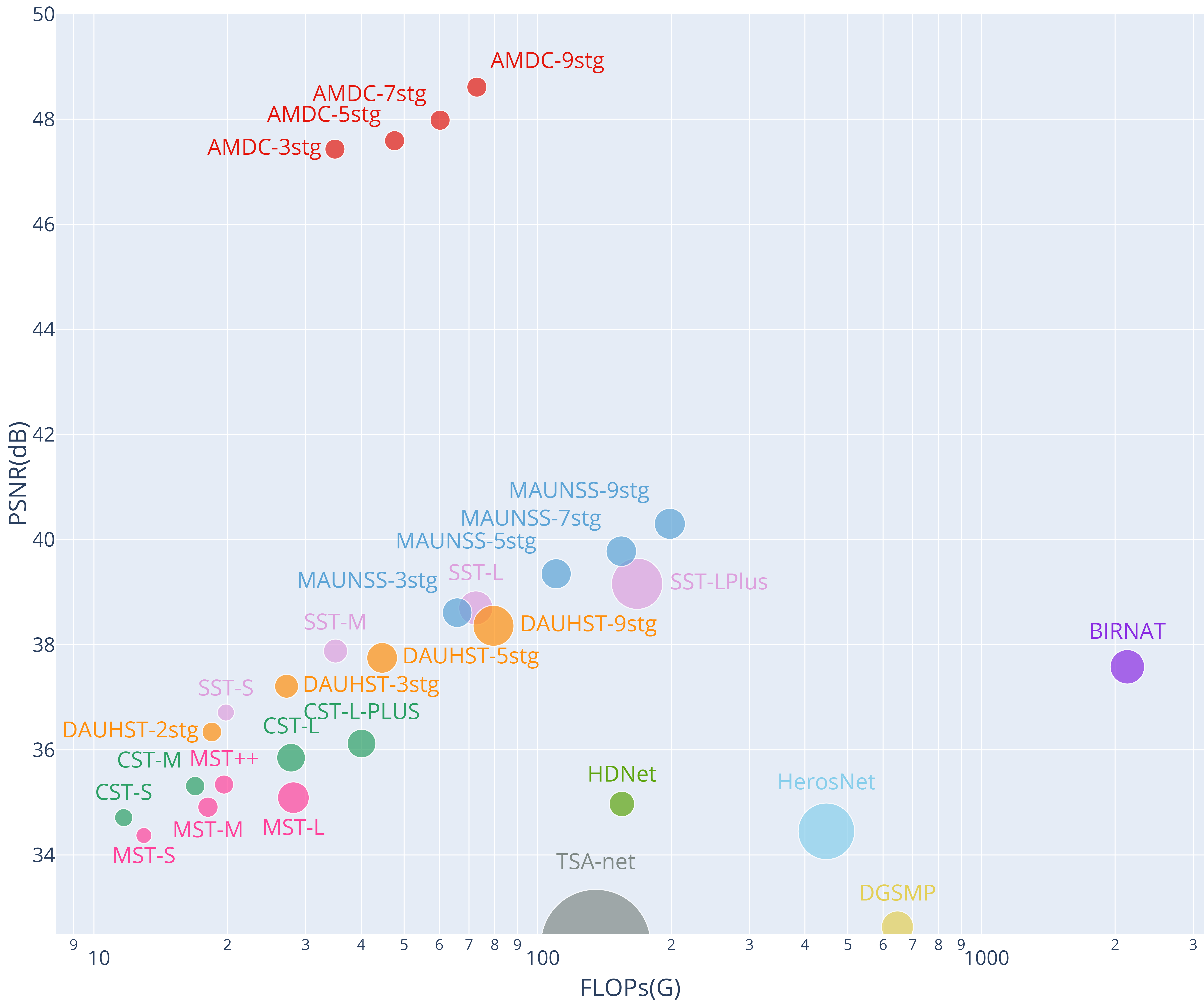
Figure 1: PSNR-parameters-FLOPs comparisons of our MLP-AMDC and SOTA HSI reconstruction methods.The vertical axis is PSNR (dB), the horizontal axis is FLOPs (computational cost), and the circle radius is parameters (memory cost).

Hyper-Spectral Image (HSI) has important applications in astrophysics, remote sensing, precision agriculture, medical biology, material identification, photogrammetry and other fields (Schechner et al. 2021; Guo, Dian, and Li 2022). Conventional hyper-spectral imaging uses line sweep, surface sweep, or rotating filters to capture HSI 3D cube. the introduction of mechanical components has resulted in a less reliable system and is not capable of capturing dynamic scenes. CASSI based on compressed sensing has theoretically demonstrated the advantages of CASSI: 1) the ability to capture HSI of dynamic scenes(Cao et al. 2016), 2) lower storage cost, and 3) more reliable lifetime without mechanical components.

However, current CASSI systems and reconstruction algorithms have two problems. 1) The MASK in CASSI either relies on random patterns or analytical design, and although existing algorithms achieve good results in these Masks, the fixed coding is not adaptive to changes in the data and more detailed textures are lost. In addition, the joint design of coding elemnets (CEs) and computational decoders is a trend in computational optical imaging (COI). Is it possible to design a multimodal adaptive coding in spectral compressed imaging to compensate for the lack of fixed coding? 2) Although the CASSI reconstruction algorithm achieves good reconstruction results, the reconstruction speed cannot meet the requirements of online reconstruction, and the existing algorithms are still offline reconstruction of HSI. how to improve the reconstruction speed without reducing the reconstruction accuracy?

To solve above problems: To further improve the reconstruction quality, in this paper, we firstly introduce Adaptive-Mask to adjust the Mask by learning the distribution of data to improve the capture capability of CASSI. Secondly, in order to reconstruct the lost detailed texture information, we introduce RGB cameras and design a dual-stream network of RGB images and CASSI images to complement each other with information from different modalities. To improve the reconstruction speed, we propose an multi-layer perceptron (MLP) Architecture for the reconstruction of spectral images, which does not use self-attention. Instead, the new architecture is based entirely on MLPs that are repeatedly applied across either spatial channels or spectral channels. To evaluate the performance of different algorithms in terms of reconstruction speed, we introduce frame rate as an evaluation metric on the dataset.

The mian contributions of this work can be summarized as follows:

• We propose a dual-camera CASSI system based on Adaptive-Mask, a multimodal CASSI system with joint optimization of CEs and decoding networks.

• We designed an MLP Architecture for hyperspectral reconstruction, and designed spectral-MLP and Swin-spatial-MLP to obtain the global correlation between CASSI measurements and RGB images, respectively, and embed them into AMDC CASSI.

• We demonstrate on several datasets that MLP, a simple structure, has no less performance than CNN, Transformer, and has faster inference, including a larger and more recent dataset (ARAD_1K). Numerous experiments have shown that our method has faster reconstruction results and reconstruction speed, and has less number of parameters and operations.

Related Work

Related works of CASSI system coding

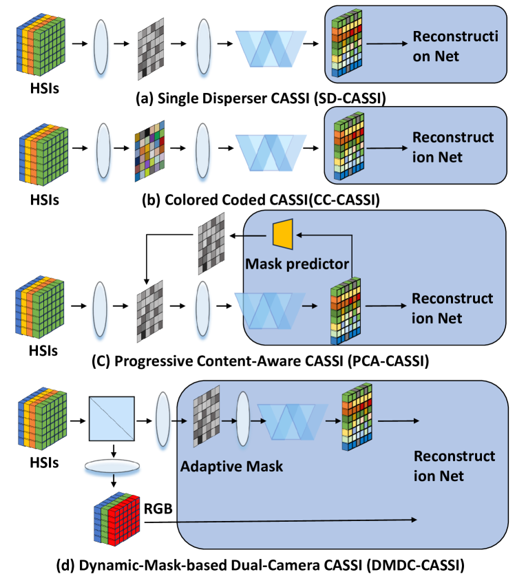
Figure 2: Detailed architecture of our MLP-AMDC.

The coding development of CASSI systems is shown in Fig. 2. A typical Single-Dispersive CASSI (SD-CASSI) design is shown in Fig. 2(a) (Wagadarikar et al. 2008), SD-CASSI utilizes a manual a priori grayscale Mask to encode the HSI, which is subsequently disperse by a dispersive device and eventually measured by the sensor. Then Dual-Dispersive CASSI (DD-CASSI) with spectral-spatial encoding (Gehm et al. 2007) and Colored Coded CASSI (CC-CASSI, Fig. 2(b)) (Arguello and Arce 2014) with multi-channel spectral encoding have been developed. Previous studies have focused on how to improve the encoding efficiency with a fixed Mask, without much consideration of the adaptation of the Mask to the data. In order to improve the effect of fixed MASK on CASSI, a multi-MASK CASSI system (MS-CASSI) at the expense of CASSI multiple imaging has been proposed (Kittle et al. 2010). Besides, Some existing works on traditional CS have explored the possibility of joint mask optimization and image reconstruction. For instance, Zhang et al. proposed a constrained optimization-inspired network (HerosNet) for adaptive sampling and recovery (Zhang et al. 2022). In the spectral SCI, Zhang et al. designed an end-to-end learnable auto-encoder to optimize the illumination pattern and compress the HSIs (Zhang et al. 2023), as shown in Fig. 2(c). However, there are fewer studies on the methods of adaptive Mask for CASSI enhancement, and the multimodal network composed of adaptive-Mask based CASSI with RGB camera inspired by DCCHI (Wang et al. 2016) has not been discussed yet. The study of joint optimization of adaptive MASK and multimodal networks is still challenging and worth exploring.

HSI reconstruction algorithms

CASSI projects HSI from 3D cube to 2D camera CCD sensor, the reconstruction problem is an ill-posed problem. HSI reconstruction algorithms can be classified into traditional methods, plug-and-play methods, End-to-End (E2E) methods, deep unfolding frameworks, and optical path reversible-based frameworks.

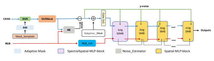
Figure 3: Detailed architecture of our MLP-AMDC.

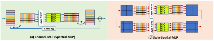
Figure 4: Detailed architecture of our MLP-AMDC.

Traditional methods are based on optimization theory and are solved by iteratively minimizing the objective function (Liu et al. 2018; Wang, Wang, and Chanussot 2021; Bioucas-Dias and Figueiredo 2007). For example, Yuan et al. used generalized alternating projection (GAP) to solve the total variation (TV) minimization problem based on the CS theory (Yuan 2016). Plug-and-play methods improve the reconstruction quality by introducing deep learning-based denoising modules into traditional methods. E2E methods are classified into CNN-based, RNN-based, and Transformer-Based methods, e.g., Zhang et al. trained a convolutional neural network (CNN)-based coded HSI reconstruction method by coded image internal learning after external learning by public HSI datasets (Zhang et al. 2019). Yang et al. introduced a symmetric residual module and a nonlocal spatial–spectral attention module into a deep learning network to capture nonlocal spatial and spectral correlations of HSI (Yang et al. 2021). Miao et al. introduced self-attention to model nonlocal features (Miao et al. 2019). Cai et al. proposed a spectral global feature extraction module of MSA-attention to obtain good reconstruction results with low parameters (Cai et al. 2022b). The depth unfolding framework replaces the convex optimization formulation by the depth module and obtains interpretable results by iterative solving. The reversible optical path-based framework reprojects each reconstruction result to the 2D measurement space, constructs new residuals with the measured values, and then minimizes the residuals by iterations to obtain results comparable to the depth unfolding framework, while having fewer parameters and operations (Cai et al. 2022d).

Methods

Model of AMDC-CASSI System

The concise AMDC-CASSI schematic is shown in Fig. 2(d). In terms of math, think about a 3D HSIs cube, denoted by $X\in\mathbb{R}^{n_{x}\times n_{y}\times n_{\lambda}}$, where $n_{x}$, $n_{y}$, $n_{\lambda}$ represent the HSIs’s height, width, and number of wavelengths. First, the scene goes through a beamsplitter. By default, the energy of the light is split evenly, and the RGB measurement, g(x,y), can be written as:

$$g\left(x,y\right)=\frac{1}{2}\int_{\Lambda}\omega\left(\lambda\right)X\left(x,y,\lambda\right)d\lambda+N$$ (1)

where$x\in n_{x},y\in n_{y},\lambda\in n_{\lambda}$, $X\left(x,y,\lambda\right)$ is the 3D hyperspectral data cube. $\Lambda$ is the spectral response range of the RGB detector. $\omega\left(\lambda\right)$ is the spectral response function of the detector. $N$ is the noise on the RGB detector.

The RGB measurements are passed through an adaptive Mask network that learns the spatial features of the scene and produces an adaptive Mask, which can be expressed as:

$$M\left(x,y\right)=AdaptiveMaskNet\left(g(x,y)\right)$$ (2)

Where $M$ denotes the Mask of CASSI. The other light path of the spectroscopic prism, which is then modulated by the adaptive mask and a dispersive prism, is finally captured by the CASSI detector. We can express it as:

$$X^{\prime}(x,y,:)=\frac{1}{2}M(x,y)\odot X(x,y,:)$$ (3)

Where $X^{\prime}\in\mathbb{R}^{n_{x}\times n_{y}\times n_{\lambda}}$ denotes the modulated spectral data cub.

$$X^{\prime\prime}(x,y,:)=X^{\prime}(x,y+d_{\lambda},:)$$ (4)

Finally, the captured 2D compressed measurement $Y\in\mathbb{R}^{n_{x}\times\left(n_{y}+d\left(n_{\lambda}-1\right)\right)}$ can be obtained by:

$$Y=\frac{1}{2}\sum_{\lambda=1}^{n_{\lambda}}M(x,y+d_{\lambda})\odot X(x,y+d_{\lambda},:)+G$$ (5)

where $G\in\mathbb{R}^{n_{x}\times\left(n_{y}+d\left(n_{\lambda}-1\right)\right)}$ is the random noise generated by the photon sensing detector during the measurement.

Combining Eq. (1) and Eq. (5) and rewriting them as linear transformations, the imaging model of dual-camera in the matrix form can be written as:

$$\begin{cases}Y_{r}=\Phi_{r}X+N_{r}\\ Y_{c}=\Phi_{c}X+N_{c}\end{cases}$$ (6)

Where $Y_{r}$ is the measurement of RGB detector. $N_{r}$ is the noise of RGB detector. $\Phi_{r}$ is the sensing matrix of RGB detector. $Y_{c}$ is the measurement of CASSI detector. $N_{c}$ is the noise of CASSI detector. $\Phi_{c}$ is the sensing matrix of CASSI detector, which is generally consider it as the shifted mask.

Overall architecture of MLP-AMDC

The observational model in Eq. (6) classifies HSI reconstruction from AMDC-CASSI and panchromatic images as an optimization problem. An observation model-derived regularization model is recommended:

$$\arg\min\left\|Y_{c}-N_{c}-\Phi_{c}X\right\|_{2}^{2}+\left\|Y_{r}-N_{r}-\Phi_{r}X\right\|_{2}^{2}$$ (7)

Equation (6) says each detector has noise. We assume that the sensor noise has the same distribution, which can be inferred from both detectors.

$$noise=\frac{\Phi_{c}^{-1}Y_{c}-\Phi_{r}^{-1}Y_{r}}{\Phi_{c}^{-1}-\Phi_{r}^{-1}}=Denoise(Y_{c},Y_{r})$$ (8)

During reconstruction, based on the optical path’s invertibility, we reproject each reconstruction’s results back into measurement space, inspired by SST-net (Cai et al. 2023). The unique solution of the forward process and the actual measurements can create residuals for the network to learn the detailed features of the spectral cube, as described by the following equation:

$$x_{n+1}=f(Y_{c}-N-\Phi_{c}x_{n},Y_{r})+x_{n}$$ (9)

where $x_{n}$ is the result of the reconstruction after the n-stage iteration. $f$ is an E2E reconstruction module that shares weighted parameters in different phases, except for the initialization phase of the reconstruction.

Adaptive mask network

As illustrated in Fig. 3, the adaptive mask network learns the spatial distribution of the scene from the dataset during training and predicts if each pixel represents redundant information. we designed the CNN-based network using the manual mask as a template. This adaptive mask network will update weights synchronously with the reconstruction network during training, then freeze and update only the reconstruction network weights, save the Mask, and delete this module during inference. Adaptive mask network:

$$M(x,y)=\mathcal{S}(\mathcal{C}(\mathcal{U}(y_{rgb}(x,y)+\mathcal{MT}(x,y))))$$ (10)

where $\mathcal{S}$ is Sigmoid function, $\mathcal{C}$ is a Convolution layer, $\mathcal{U}$ is a u-net, $\mathcal{MT}$ is the Mask Template.

Multimodal reconstruction network

The function of the multimodal reconstruction network is to reconstruct the spectral 3D cube from the RGB and CASSI measurements. As shown in Fig. 3, the reconstruction network uses a dual-stream architecture and constructs a residual learning network of Eq. (9) based on the reversible nature of the optical path, and reconstitutes the input of n+1 stage using the results of the n-stage to improve the reconstruction quality. The key modules of the Subnet are Noise-Estimator module (NE), RGB-init module, Swin-Spatial-MLP block and SpectralSpatial MLP block. First, the network predicts the noise distribution of the detector by the NE module and corrects the CASSI data. Subsequently, the job of the RGB initialization module is to transfer RGB to a higher dimensional space, synchronize the number of RGB channels with the number of CASSI channels, and assist in learning the long-range correlations of RGB branches in each channel. Finally, the dual-stream data are iterated to learn the entire correlation of the spectrum and the full correlation of the space.

Noise-Estimator module (NE). We presume that the distribution function of the noise on the RGB detector and the CASSI detector is the same. The NE module transfers the RGB and CASSI branches to a high-dimensional space, learns the noise distribution, downscales it to the original space, and then estimates the noise using the imbalance data between the two branches. The following is a description of this procedure:

$$N=\mathcal{O}(\mathcal{D}(\mathcal{C}(Up(x_{c}))))-\mathcal{O}(\mathcal{D}(\mathcal{C}(Up(x_{r}))))+\varepsilon$$ (11)

where $N$ is the estimated noise, $\mathcal{O}$ is a Softmax layer, $\mathcal{D}$ is a downsampling layer, $\mathcal{C}$ is a Convolution layer, Up is a upsampling layer.

RGB-init module. RGB initialization module that scales raw RGB measurements to 64 dimensions before downscaling them to original channels, allowing RGB measurements to be aligned with CASSI channel counts.

SpectralSpatial MLP block. Because C¡¡W=H, Channel-MLP has the lowest reconstruction cost and is suited for CASSI branch and RGB branch initiation. Swin-Spatial-MLP learns the global similarity of the two branches in space using spectral characteristics.

Spatial MLP block. The residuals of the measurement and the n-stage reconstruction results are constructed, the Swin-Spatial-MLP is utilized to learn the global correlation between the residuals and the RGB images in space.

Loss function

Our network has reversible module and reconstruction net, so our loss includes outputting and reversible loss. The outputting loss is calculated as the L2 loss of $x_{out}$ - $x_{truth}$. The reversible loss calculation $x_{out}$ is mapped back to the CCD under the nature of the reversible optical path to obtain the L2 loss of the G ($x_{out}$) value to the actual measurement y. We defined the loss function as follows:

$$\mathcal{L}=\left\|\widehat{x}_{out}-x_{truth}\right\|_{2}^{2}+\xi\cdot\left\|\Phi\widehat{x}_{out}-x_{in}\right\|_{2}^{2}$$ (12)

where $\widehat{x}_{out}$ is the predicted values of the network, $\Phi$ represents the process of mask coding and dispersion of predicted values, $x_{in}$ is the measurement of CCD. $\xi$ is the penalty coefficient.

Table 1: Comparisons between MLP-AMDC and SOTA methods on 10 simulation scenes (S1$\sim$S10) in KAIST. PSNR and SSIM are reported.

	$\lambda$	ADMM	TSA	Gap	DGS	PnP-DIP	BIR	HD	MST	CST	Heros	DAUHST	SST	RDLUF	AMDC
	-net	-Net	-net	-net	MP	-HSI	NAT	Net	++	-L	Net	-9stg	-LPlus	-9stage	-9stg
PSNR	31.77	33.58	32.30	24.36	32.63	31.26	37.58	34.97	35.34	36.12	34.45	38.36	39.16	39.57	48.61
SSIM	89.0%	91.8%	91.6%	66.9%	91.7%	89.4%	96.0%	94.3%	95.3%	95.7%	97.0%	96.7%	97.4%	97.4%	99.6%

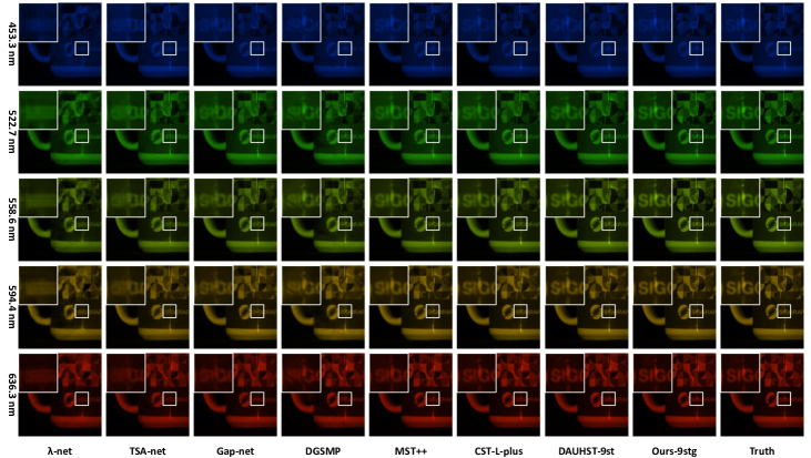
Figure 5: Visual comparisons of our MLP-ADAM and other SOTA methods of Scene 5 with 5 out of 28 spectral channels on the KAIST dataset.

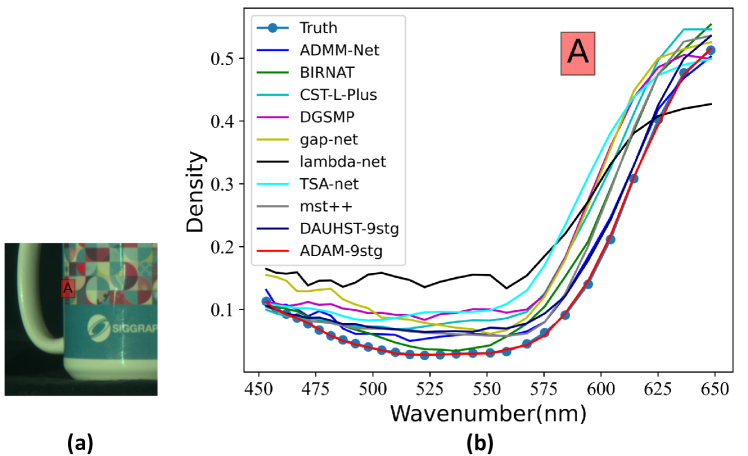
Figure 6: Spectral curves on the selected regions (A) and the visualization results show that our results have higher spectral accuracy and better perceptual quality.

Figure 7: Comparison of FPS and PSNR for AMDCs and other SOTA methods.

Experiments

This section shows how the proposed SOTA reconstruction method outperforms others on numerous datasets, including re-evaluating the SOTA model in CASSI on the current dataset ARAD_1K.

Experiment Setup

CAVE (Park et al. 2007) and KAIST’s (Choi et al. 2017) testing dataset has 28 spectral channels, ranging from 450 to 650 nm. CAVE and KAIST simulation hyperspectral image datasets are used. CAVE dataset has 32$\times$ 512 $\times$ 512 hyperspectral pictures. 30 hyperspectral photos from KAIST are 2704 $\times$ 3376. CAVE is the training set, following TSA-Net’s schedule (Meng, Ma, and Yuan 2020). Test 10 KAIST scenes.

ARAD_1K presents a larger-than-ever natural hyperspectral image dataset. This data collection approximately doubles the ARAD_1K HS data set to 1,000 pictures. ARAD_1K has 31 hyperspectral images at 482 $\times$ 512 from 400 to 700 nm with a 10 nm increment. The 1,000 data set photos were divided: 900 training, 50 validation, and 50 test photos (Arad et al. 2022).

We select peak signal-to-noise ratio (PSNR), structural similarity (SSIM)(Wang et al. 2004), Mean Relative Absolute Error (MRAE) and Root Mean Square Error (RMSE) as the metrics to evaluate the HSI reconstruction performance. CAVE and KAIST continue to use PSNR, SSIM, parameters, and floating point numbers as evaluation measures. MRAE is ARAD_1K’s major metric.

We implement MLP-AMDC in Pytorch. All mrthods are trained on 1 $\times$ RTX 3090 GPU. Adam(Kingma and Ba 2014) optimizer for 300 epochs ($\beta_{1}=0.9$ and $\beta_{2}=0.999$). The training rate starts at $4\times 10^{-4}$ and is halved every 50 epochs.

Table 2: Comparisons between MLP-AMDC and SOTA methods on 50 scenes in ARAD_1K. MRAE, RMSE, PSNR, SSIM , parameters, FLOPS and reconstruction time are reported.

method	Avg MRAE	Avg RMSE	Avg PSNR	Avg SSIM	Params(M)	GFLOPS(G)	Time for 50 pics (s)
$\lambda$-net	0.1664	0.0228	33.29	91.63%	32.73	31.18	0.19
TSA-net	0.1392	0.0193	34.82	93.82%	44.30	142.34	0.53
Gap-net	0.3005	0.0466	27.02	84.26%	4.28	87.55	1.10
Admm-net	0.2949	0.0475	27.03	84.22%	4.28	87.55	1.02
MST-S	0.0984	0.0135	37.93	96.51%	1.12	14.93	0.77
MST-M	0.0855	0.0119	39.02	97.21%	1.81	20.85	1.33
MST-L	0.0776	0.0102	40.64	97.71%	2.45	32.18	1.97
MST++	0.0936	0.0127	38.49	96.92%	1.63	23.88	0.55
CST-S	0.1308	0.0165	36.25	95.23%	1.46	12.21	0.64
CST-M	0.1147	0.0153	36.91	95.77%	1.66	15.96	1.17
CST-L	0.0956	0.0125	38.95	96.74%	3.66	27.17	1.68
CST-LPlus	0.0854	0.0115	39.63	97.16%	3.66	33.95	2.15
DAUHST-3stg	0.0686	0.0094	41.31	97.90%	1.64	29.13	0.99
DAUHST-5stg	0.0590	0.0076	43.89	98.36%	2.70	47.72	1.50
DAUHST-7stg	0.0575	0.0074	44.20	98.44%	3.77	66.32	3.62
DAUHST-9stg	0.0602	0.0073	44.18	98.45%	4.83	84.92	4.42
AMDC-1stg	0.0710	0.0077	43.28	98.59%	1.25	25.81	0.34
AMDC-3stg	0.0432	0.0046	47.15	99.34%	1.77	41.28	0.71
AMDC-5stg	0.0429	0.0046	47.47	99.34%	1.77	56.75	1.59
AMDC-7stg	0.0442	0.0045	47.75	99.32%	1.77	72.23	2.49
AMDC-9stg	0.0420	0.0044	47.99	99.35%	1.77	87.80	3.54

results on CAVE and KAIST

(i)On CAVE and KAIST, our best model AMDC-9stg yields very impressive results, i.e., 48.61 dB in PSNR and 99.6% in SSIM ,which is more than 9 dB than the best PSNR of the SOTA published models, and the SSIM is more than 2.2%. AMDC-9stg significantly outperforms RDLUF-9stage (Dong et al. 2023), SST-LPlus (Cai et al. 2023), DAUHST-9stg (Cai et al. 2022d), HerosNet (Zhang et al. 2022), CST-L (Cai et al. 2022a), MST++ (Cai et al. 2022c), HDNet (Hu et al. 2022), BIRNAT (Cheng et al. 2022), PnP-DIP-HSI (Meng et al. 2021), DGSMP (Huang et al. 2021), GAp-net (Meng, Jalali, and Yuan 2020), TSA-net (Meng, Ma, and Yuan 2020), ADMM-Net (Ma et al. 2019), and $\lambda$-net (Miao et al. 2019) of PSNR by 9.04, 9.45, 10.25, 14.16, 12.49, 13.27, 13.64, 11.03, 17.35, 15.98, 24.25, 16.31, 15.03 and 16.84 dB, and 2.2%, 2.2%, 2.9%, 2.6%, 3.9%, 4.3%, 5.3%, 3.6%, 10.2%, 7.9% , 32.7% , 8.0% , 7.8% , and 10.6% improvement of SSIM. Detailed comparison data are shown in Table 1, See appendix for detailed data.

Table 3: Evaluation of the effectiveness of different components.

Base-line	Adaptive Mask	RGB	Noise Estimator	MRAE	RMSE	PSNR	SSIM	Params	GFLOPs
				Avg	Avg	Avg(dB)	Avg	(M)
AMDC-3stg	$\surd$	$\surd$	$\times$	0.0459	0.0049	46.71	99.27%	1.67	34.69
AMDC-3stg	$\surd$	$\times$	$\surd$	0.0668	0.0070	43.65	98.71%	0.69	17.05
AMDC-3stg	$\surd$	$\surd$	$\surd$	0.0432	0.0046	47.15	99.34%	1.77	41.28

Table 4: Evaluation of the performance between MLP and transformer.

Base-line	backbone	Avg MRAE	Avg RMSE	Avg PSNR	Avg SSIM	Params	GFLOPs	FPS
				(dB)		(M)
AMDC-3stg	Transformer	0.0488	0.0052	46.22	99.28%	1.93	45.08	45.8
AMDC-5stg	Transformer	0.0453	0.0049	46.64	99.33%	1.93	63.62	22.0
AMDC-7stg	Transformer	0.0455	0.0048	47.32	99.31%	1.93	82.15	14.6
AMDC-9stg	Transformer	0.0430	0.0044	47.85	99.38%	1.93	100.69	11.1
AMDC-3stg	MLP	0.0432	0.0046	47.15	99.34%	1.77	41.28	70.4
AMDC-5stg	MLP	0.0429	0.0046	47.20	99.34%	1.77	56.75	31.5
AMDC-7stg	MLP	0.0442	0.0045	47.75	99.32%	1.77	72.23	20.88
AMDC-9stg	MLP	0.0421	0.0044	47.99	99.35%	1.77	87.80	14.12

Table 5: Evaluation of the effectiveness of different types of Mask.

Base-line	Mask type	Avg MRAE	Avg RMSE	Avg PSNR	Avg SSIM	Params	GFLOPs
				(dB)
AMDC-3stg	Manual Prior Mask	0.0582	0.0067	44.03	98.81%	1.77	41.28
AMDC-3stg	Rand Mask	0.0504	0.0057	45.47	99.09%	1.77	41.28
AMDC-3stg	Normal Mask	0.0515	0.0056	45.60	99.13%	1.77	41.28
AMDC-3stg	Aynamic Mask	0.0432	0.0046	47.15	99.34%	1.77	41.28

(ii)It can be observed that our MLP-AMDC significantly surpass SOTA methods by a large margin while requiring much cheaper memory and computational costs. Compared with DU methods, AMDC-5stg outperforms RDLUF-9stage by 7.90 db but only costs 79.4% (1.47/1.85) parameters and 39.6% (47.59/120.08) FLOPs, outperforms DAUHST-9stg 9.11 db but only costs 23.9% (1.47/6.15) parameters and 57.3% (47.59/79.50) FLOPs. And outperforms other Transformer-based methods, our AMDC-1stg outperforms CST-L (Cai et al. 2022a) by 4.36 dB but only costs 34.6% (1.04/3.00) Params and 79.7% (22.18/27.81) FLOPs, and AMDC-1stg outperforms MST++ (Cai et al. 2022b) by 4.87 dB, but only costs 28.4% (1.04/3.66) Params and 78.8% (22.18/28.15) FLOPs. In addition, our AMDC-3stg, AMDC-5stg, AMDC-7stg and AMDC-9stg outperforms other competitors by very large margins. we provide PSNR-parameters-FLOPs comparisons of different reconstruction algorithms in Fig. 1.

Fig. 5 plots the visual comparisons of our AMDC-9stg and other SOTA methods on Scene 3 with 5 (out of 28) spectral channels. The top-left part shows the zoomed-in patches of the white boxes in the entire HSIs, the reconstructed HSIs produced by AMDCs have more spatial details and clearer texture in different spectral channels than other SOTA methods. In addition, the spectral curves of the AMDCs have a higher correlation with the reference spectra in the quantitative spectral data. As shown in Fig. 6(b) with the red line and the blue line.

Results on ARAD_1K

On ARAD_1K, the comparison data of AMDC and SOTA models are shown in Table 2, our AMDC-9stg yields 0.0420 in MRAE, 0.0044 in RMSE, 47.99 in PSNR, 99.35% in SSIM. AMDC-9stg still significantly outperforms DAUHST-9stg (Cai et al. 2022d), CST-LPlus (Cai et al. 2022a), MST++ (Cai et al. 2022c), Admm-net (Ma et al. 2019), Gap-net (Meng, Jalali, and Yuan 2020), TSA-net (Meng, Ma, and Yuan 2020), and $\lambda$-net (Miao et al. 2019) of MRAE by 0.0182, 0.0434, 0.0516, 0.2529, 0.2585, 0.0972, and 0.1244, and of PSNR by 3.45, 8.36, 9.50, 20.96, 20.97, 13.17, and 14.70, and 0.90%, 2.09%, 2.43%, 15.13%, 15.09%, 5.53%, and 7.72% improvement of SSIM, suggesting the effectiveness of our method.

Ablation study

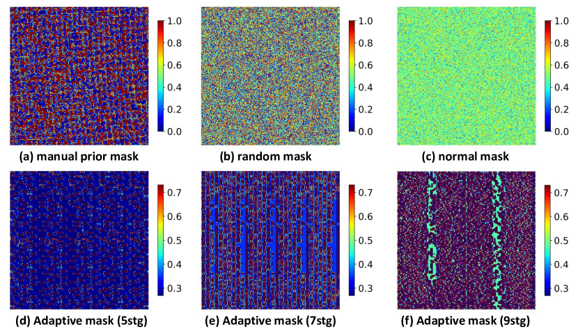
Figure 8: Comparison of manual prior mask, random mask, normal mask and dynamic mask.

Ablation analysis using ARAD_1K datasets evaluates the proposed AMDCs’ components. Adaptive mask, RGB branching, Noise Estimator, and MLP vs. transformer performance are our key focus. Tab. 3, tab. 4 and tab. 5 displays MRAE, RMSE, PSNR, and SSIM for RGB ranching and Noise Estimator settings, different AMDC sizes, and different mask methods.The adaptive mask and RGB branching increase the network equally. The difference between adaptive mask and other masks is shown in Fig. 8. Adaptive mask has a better encoding method based on RGB prior.

To evaluate the combined comparison of the reconstruction speed and performance of different algorithms on ARAD_1K, we analyzed the PSNR and FPS of SOTA methods. As shown in Fig. 7, our AMDC-1stg is ten as fast for the same reconstruction quality, as well as other AMDCs.

Conclusion

This study proposes AMDC, a CASSI framework. The new approach addresses the problem of random and manual masks not fitting the dataset, which lowers reconstruction performance, and the transformer-based method is slower and more arithmetic. We present an MLP-AMDC with adaptive mask and multimodal reconstruction networks to integrate CASSI data with RGB photos using AMDC-CASSI. These unique methods provide very efficient MLP-AMDC models. Our technique outperforms SOTA algorithms even with cheaper settings and FLOPs.

References

- Arad et al. (2022) Arad, B.; Timofte, R.; Yahel, R.; Morag, N.; Bernat, A.; Cai, Y.; Lin, J.; Lin, Z.; Wang, H.; Zhang, Y.; et al. 2022. Ntire 2022 spectral recovery challenge and data set. In Proceedings of the IEEE/CVF Conference on Computer Vision and Pattern Recognition, 863–881.
- Arguello and Arce (2014) Arguello, H.; and Arce, G. R. 2014. Colored coded aperture design by concentration of measure in compressive spectral imaging. IEEE Transactions on Image Processing, 23(4): 1896–1908.
- Bioucas-Dias and Figueiredo (2007) Bioucas-Dias, J. M.; and Figueiredo, M. A. 2007. A new TwIST: Two-step iterative shrinkage/thresholding algorithms for image restoration. TIP, 16(12): 2992–3004.
- Cai et al. (2022a) Cai, Y.; Lin, J.; Hu, X.; Wang, H.; Yuan, X.; Zhang, Y.; Timofte, R.; and Van Gool, L. 2022a. Coarse-to-fine sparse transformer for hyperspectral image reconstruction. 686–704.
- Cai et al. (2022b) Cai, Y.; Lin, J.; Hu, X.; Wang, H.; Yuan, X.; Zhang, Y.; Timofte, R.; and Van Gool, L. 2022b. Mask-guided spectral-wise transformer for efficient hyperspectral image reconstruction. In CVPR, 17502–17511.
- Cai et al. (2022c) Cai, Y.; Lin, J.; Lin, Z.; Wang, H.; Zhang, Y.; Pfister, H.; Timofte, R.; and Van Gool, L. 2022c. Mst++: Multi-stage spectral-wise transformer for efficient spectral reconstruction. In CVPR, 745–755.
- Cai et al. (2022d) Cai, Y.; Lin, J.; Wang, H.; Yuan, X.; Ding, H.; Zhang, Y.; Timofte, R.; and Van Gool, L. 2022d. Degradation-Aware Unfolding Half-Shuffle Transformer for Spectral Compressive Imaging. NeurIPS.
- Cai et al. (2023) Cai, Z.; Yu, J.; Zhang, Z.; Jin, C.; and Da, F. 2023. SST-ReversibleNet: Reversible-prior-based Spectral-Spatial Transformer for Efficient Hyperspectral Image Reconstruction. arXiv preprint arXiv:2305.04054.
- Cao et al. (2016) Cao, X.; Yue, T.; Lin, X.; Lin, S.; Yuan, X.; Dai, Q.; Carin, L.; and Brady, D. J. 2016. Computational snapshot multispectral cameras: Toward dynamic capture of the spectral world. IEEE Signal Processing Magazine, 33(5): 95–108.
- Cheng et al. (2022) Cheng, Z.; Chen, B.; Lu, R.; Wang, Z.; Zhang, H.; Meng, Z.; and Yuan, X. 2022. Recurrent neural networks for snapshot compressive imaging. TPAMI.
- Choi et al. (2017) Choi, I.; Kim, M.; Gutierrez, D.; Jeon, D.; and Nam, G. 2017. High-quality hyperspectral reconstruction using a spectral prior. TOG, 36(6): 218.
- Dong et al. (2023) Dong, Y.; Gao, D.; Qiu, T.; Li, Y.; Yang, M.; and Shi, G. 2023. Residual Degradation Learning Unfolding Framework With Mixing Priors Across Spectral and Spatial for Compressive Spectral Imaging. In Proceedings of the IEEE/CVF Conference on Computer Vision and Pattern Recognition (CVPR), 22262–22271.
- Gehm et al. (2007) Gehm, M. E.; John, R.; Brady, D. J.; Willett, R. M.; and Schulz, T. J. 2007. Single-shot compressive spectral imaging with a dual-disperser architecture. Optics express, 15(21): 14013–14027.
- Guo, Dian, and Li (2022) Guo, A.; Dian, R.; and Li, S. 2022. A Deep Framework for Hyperspectral Image Fusion between Different Satellites. IEEE Transactions on Pattern Analysis and Machine Intelligence.
- Hu et al. (2022) Hu, X.; Cai, Y.; Lin, J.; Wang, H.; Yuan, X.; Zhang, Y.; Timofte, R.; and Van Gool, L. 2022. Hdnet: High-resolution dual-domain learning for spectral compressive imaging. In CVPR, 17542–17551.
- Huang et al. (2021) Huang, T.; Dong, W.; Yuan, X.; Wu, J.; and Shi, G. 2021. Deep gaussian scale mixture prior for spectral compressive imaging. In CVPR, 16216–16225.
- Kingma and Ba (2014) Kingma, D. P.; and Ba, J. 2014. Adam: A method for stochastic optimization. arXiv preprint arXiv:1412.6980.
- Kittle et al. (2010) Kittle, D.; Choi, K.; Wagadarikar, A.; and Brady, D. J. 2010. Multiframe image estimation for coded aperture snapshot spectral imagers. Applied optics, 49(36): 6824–6833.
- Liu et al. (2018) Liu, Y.; Yuan, X.; Suo, J.; Brady, D. J.; and Dai, Q. 2018. Rank minimization for snapshot compressive imaging. TPAMI, 41(12): 2990–3006.
- Ma et al. (2019) Ma, J.; Liu, X.-Y.; Shou, Z.; and Yuan, X. 2019. Deep tensor admm-net for snapshot compressive imaging. In Proceedings of the IEEE/CVF International Conference on Computer Vision, 10223–10232.
- Meng, Jalali, and Yuan (2020) Meng, Z.; Jalali, S.; and Yuan, X. 2020. Gap-net for snapshot compressive imaging. arXiv preprint arXiv:2012.08364.
- Meng, Ma, and Yuan (2020) Meng, Z.; Ma, J.; and Yuan, X. 2020. End-to-end low cost compressive spectral imaging with spatial-spectral self-attention. In ECCV, 187–204.
- Meng et al. (2021) Meng, Z.; Yu, Z.; Xu, K.; and Yuan, X. 2021. Self-supervised neural networks for spectral snapshot compressive imaging. In Proceedings of the IEEE/CVF International Conference on Computer Vision, 2622–2631.
- Miao et al. (2019) Miao, X.; Yuan, X.; Pu, Y.; and Athitsos, V. 2019. l-net: Reconstruct hyperspectral images from a snapshot measurement. In ICCV, 4059–4069.
- Park et al. (2007) Park, J.-I.; Lee, M.-H.; Grossberg, M. D.; and Nayar, S. K. 2007. Multispectral imaging using multiplexed illumination. In ICCV, 1–8.
- Schechner et al. (2021) Schechner, Y. Y.; Bala, K.; Katz, O.; Sunkavalli, K.; and Nishino, K. 2021. Guest Editorial: Introduction to the Special Section on Computational Photography. IEEE Transactions on Pattern Analysis and Machine Intelligence, 43(7): 2175–2178.
- Wagadarikar et al. (2008) Wagadarikar, A.; John, R.; Willett, R.; and Brady, D. 2008. Single disperser design for coded aperture snapshot spectral imaging. Applied optics, 47(10): B44–B51.
- Wang et al. (2016) Wang, L.; Xiong, Z.; Shi, G.; Wu, F.; and Zeng, W. 2016. Adaptive nonlocal sparse representation for dual-camera compressive hyperspectral imaging. IEEE transactions on pattern analysis and machine intelligence, 39(10): 2104–2111.
- Wang, Wang, and Chanussot (2021) Wang, M.; Wang, Q.; and Chanussot, J. 2021. Tensor Low-Rank Constraint and Total Variation for Hyperspectral Image Mixed Noise Removal. IEEE Journal of Selected Topics in Signal Processing, 15(3): 718–733.
- Wang et al. (2004) Wang, Z.; Bovik, A. C.; Sheikh, H. R.; and Simoncelli, E. P. 2004. Image quality assessment: from error visibility to structural similarity. TIP, 13(4): 600–612.
- Yang et al. (2021) Yang, Y.; Xie, Y.; Chen, X.; and Sun, Y. 2021. Hyperspectral snapshot compressive imaging with non-local spatial-spectral residual network. Remote Sensing, 13(9): 1812.
- Yuan (2016) Yuan, X. 2016. Generalized alternating projection based total variation minimization for compressive sensing. In 2016 IEEE International conference on image processing (ICIP), 2539–2543. IEEE.
- Zhang et al. (2019) Zhang, T.; Fu, Y.; Wang, L.; and Huang, H. 2019. Hyperspectral image reconstruction using deep external and internal learning. In Proceedings of the IEEE/CVF International Conference on Computer Vision, 8559–8568.
- Zhang et al. (2023) Zhang, X.; Chen, B.; Zou, W.; Liu, S.; Zhang, Y.; Xiong, R.; and Zhang, J. 2023. Progressive Content-aware Coded Hyperspectral Compressive Imaging. arXiv preprint arXiv:2303.09773.
- Zhang et al. (2022) Zhang, X.; Zhang, Y.; Xiong, R.; Sun, Q.; and Zhang, J. 2022. Herosnet: Hyperspectral explicable reconstruction and optimal sampling deep network for snapshot compressive imaging. In Proceedings of the IEEE/CVF Conference on Computer Vision and Pattern Recognition, 17532–17541.