Reset It and Forget It: Relearning Last-Layer Weights Improves Continual and Transfer Learning

Abstract

This work identifies a simple pre-training mechanism that leads to representations exhibiting better continual and transfer learning. This mechanism—the repeated resetting of weights in the last layer, which we nickname “zapping”—was originally designed for a meta-continual-learning procedure, yet we show it is surprisingly applicable in many settings beyond both meta-learning and continual learning. In our experiments, we wish to transfer a pre-trained image classifier to a new set of classes, in a few shots. We show that our zapping procedure results in improved transfer accuracy and/or more rapid adaptation in both standard fine-tuning and continual learning settings, while being simple to implement and computationally efficient. In many cases, we achieve performance on par with state of the art meta-learning without needing the expensive higher-order gradients, by using a combination of zapping and sequential learning. An intuitive explanation for the effectiveness of this zapping procedure is that representations trained with repeated zapping learn features that are capable of rapidly adapting to newly initialized classifiers. Such an approach may be considered a computationally cheaper type of, or alternative to, meta-learning rapidly adaptable features with higher-order gradients. This adds to recent work on the usefulness of resetting neural network parameters during training, and invites further investigation of this mechanism.

1 Introduction

Biological creatures display astounding robustness, adaptability, and sample efficiency—while artificial systems suffer catastrophic forgetting or struggle to generalize far beyond the distribution of their training examples. It has been observed in biological systems that repeated exposure to stressors can result in the evolution of more robust phenotypes (Rohlf & Winkler, 2009; Félix & Wagner, 2008). However, it is not clear what type of stressor during the training of a neural network would most effectively, or efficiently, convey robustness and adaptability to that system at test time.

It is common practice to have the training of a machine learning system mimic the desired use-cases at test time as closely as possible. In the case of an image classifier, this would include drawing independent training samples from a distribution identical to the test set (i.i.d. training). When the test scenario is itself a learning process—such as few-shot transfer learning from a limited number of novel examples—training can include repeated episodes of rapid adaptation to small subsets of the whole dataset, thereby mimicking the test scenario. Meta-learning algorithms (learning to learn) for such contexts are able to identify patterns that generalize across individual learning episodes (Schmidhuber, 1987; Bengio et al., 1990; Hochreiter et al., 2001; Ravi & Larochelle, 2017; Finn et al., 2017).

Going even further, we are interested in challenging scenarios of online/continual learning with few examples per class. Recent work by Javed & White (2019) and Beaulieu et al. (2020) has tackled this challenging setting with the application of meta-learning. When the learning process itself is differentiable, one way to perform meta-optimization is by differentiating through several model updates using second-order gradients, as is done in MAML (Finn et al., 2017). When applied to episodes of continual learning, this approach introduces an implicit regularization strategy (it penalizes weight changes that are disruptive to previously learned concepts, without needing a separate heuristic to quantify the disruption).

OML (Javed & White, 2019) divide their architecture into two parts, where later layers are updated in a fast inner loop but earlier layers are only updated in a slower outer meta-update. Subsequently, ANML (Beaulieu et al., 2020) restructured the OML setup by moving the earlier meta-only layers into a parallel neuromodulatory path which meta-learned an attention-like context-dependent multiplicative gating, achieving state of the art performance in sequential transfer.

However, in this work we show that neither the asymmetric training of different parts of the network (like OML), nor a neuromodulatory path (like ANML), nor even expensive second-order updates (like both), are necessary to achieve equivalent performance in this setting. Instead, we reveal that the key contribution of the OML-objective appears to be a previously overlooked mechanism: a weight resetting and relearning procedure, which we call “zapping”. This procedure consists of frequent random resampling of the weights leading into one or more output nodes of a deep neural network, which we refer to as “zapping” those neurons.

After reinitializing the last layer weights, the gradients for the weights in upstream layers quantify how the representation should have been different to reduce the loss given a new set of random weights. This is exactly the situation that the representation will find itself in during transfer. In the case where all weights of the last layer are reset, zapping closely matches transfer learning (when using the common technique of resetting the classifier layer(s) on top of pre-trained feature extraction layers; Yosinski et al. (2014)). Over multiple repetitions, this leads to representations which are more suitable for transfer.

We show that:

• Dedicating second-order optimization paths for certain layers isn’t necessary and doesn’t explain the performance of meta-learning for continual transfer (Section 3.1).

• The zapping forget-and-relearn mechanism accounts for the majority of the meta-learning improvements observed, and can be useful even without much more expensive higher-order gradients (Section 3.2).

• Representations learned by models pre-trained using zapping are better for general transfer learning, not just continual learning (Section 3.3).

2 Methods

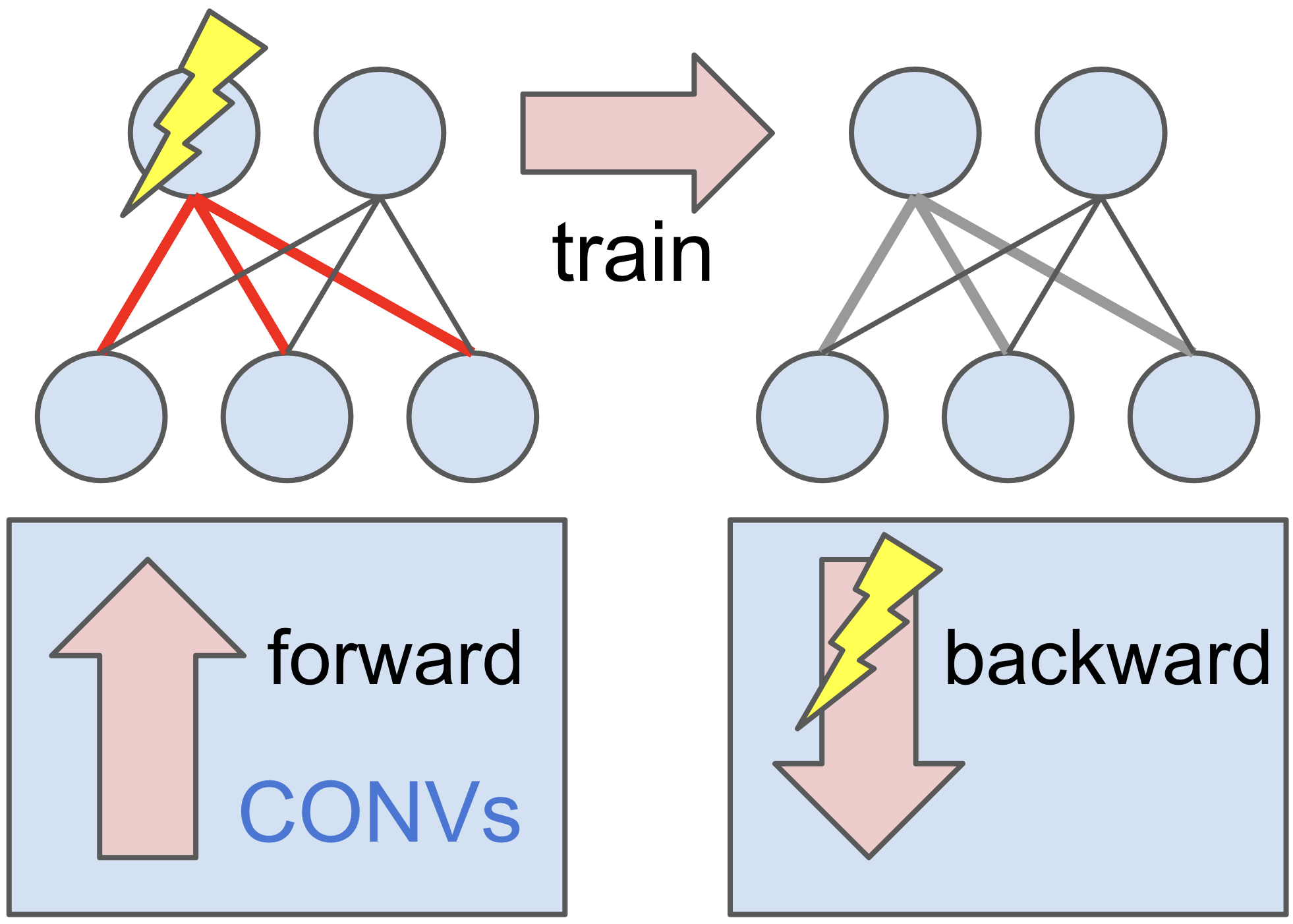
Figure 1: The effect of ↯ zapping an existing class is backpropagated to lower layers.

As described in Javed & White (2019) and Beaulieu et al. (2020), we seek to train a model capable of learning a large number of tasks $\mathcal{T}_{1..n}$, in a few shots per task, with many model updates occurring as tasks are presented sequentially. Tasks $\mathcal{T}_{i}$ come from a common domain $\mathcal{D}$. In our experiments we consider the domain to be a natural images dataset and tasks to be individual classes $\mathcal{C}_{i}$ in that dataset.

Deep learning models learn hierarchical representations but the exact contribution of each individual level in the hierarchy is still under active research. Recent works show that reinitialization of layers during training can be used as a regularization method (Zhao et al., 2018; Li et al., 2020; Alabdulmohsin et al., 2021; Zhou et al., 2022). But there are several ways in which this reinitialization can be applied. We focus our attention on the last fully connected layer, right before the output. While the information value within this last layer may be marginal (Hoffer et al., 2018) interventions in the last layer will affect the gradient calculation of all the other layers in the network during backpropagation (see Figure 1).

Our model consists of a small convolutional network with two main parts: a stack of convolutional layers that act as a feature extractor, and a single fully connected layer that acts as a linear classifier using the extracted features (see Appendix D, Figure 9). Our “zapping" procedure consists of re-sampling all the connections corresponding to one of the output classes. Because of the targeted disruption of the weights, the model suddenly forgets how to map the features extracted by previous convolutional layers to the correct class. To recover from this sudden change, the model is shown examples from the forgotten class, one at a time. By taking several optimization steps, the model recovers from the negative effect of zapping. This procedure constitutes the inner loop in our meta-learning setup and is followed by an outer loop update using examples from all classes (Javed & White, 2019). The outer loop update is done with a higher-order gradient w.r.t. to the initial weights of that inner loop iteration (Finn et al., 2017). But, as we will see, these inner and outer updates do not actually need to be performed in a nested loop—they can also be arranged in a flat sequence, yielding similar performance with much more efficient training.

2.1 Training Phases

Since we want to learn each class in just a few shots, it behooves us to start with a pre-trained model rather than starting tabula rasa. Therefore our problem set-up involves two stages. Within each stage, we examine multiple possible configuration options, described in more detail in the next sections.

1. (Sec. 2.1.1) Pre-Training: We use one of the following algorithms to train on a subset of classes: (1) standard i.i.d. pre-training, (2) alternating sequential and batch learning (ASB), or (3) meta-learning through sequential and batch learning (meta-ASB). Each of these may or may not include the zapping procedure to forget and relearn.

2. (Sec. 2.1.2) Transfer: Following pre-training, we transfer the classifier to a separate subset of classes using (1) sequential transfer (continual learning) or (2) standard i.i.d. transfer (fine-tuning).

2.1.1 Stage 1: Pre-Training

Our pre-training algorithm is described in Algorithm 1, and visualized in Appendix E, Figure 10. Our algorithm is based on the “online-aware” meta-learning (OML, Javed & White (2019)) procedure, which consists of two main components:

• Adapting (inner loop; sequential learning): In this phase the learner is sequentially shown a set of examples from a single random class and trained using standard SGD. The examples are shown one at a time, so that the optimization performs one SGD step per image.

• Remembering (outer loop; batch learning): After each adapting phase, the most recent class plus a random sample from all classes are used to perform a single outer-loop batch update. Those samples serve as a proxy of the true meta-loss (learning new things without forgetting anything already learned). The gradient update is taken w.r.t. the initial inner-loop parameters, and those updated initial weights are then used to begin the next inner-loop adaptation phase following the MAML paradigm (Finn et al., 2017).

Compared to OML we use a different neural architecture (which improves classification performance; Appendix D, Figure 9), and do not draw a distinction between when to update the feature extraction vs. classification layers (updating both in the inner and outer loops). Furthermore, while the original OML procedure included both zapping and higher-order gradients, we ablate the effect of each component by allowing them to be turned on/off as follows.

In configurations with zapping (denoted as zap in Algorithm 1), prior to each sequential adaption phase on a single class $\mathcal{C}_{i}$, the final layer weights corresponding to that class are re-initialized—in other words, they are re-sampled from the initial weight distribution. We call this procedure zapping as it destroys previously learned knowledge that was stored in those connections.

In the meta-learning conditions (denoted as meta in Algorithm 1), the “remembering” update is performed as an outer-loop meta-update on the initial weights of each inner-loop (as described above). However, we also wish to examine the effect of zapping independent of meta-learning, and introduce a new pre-training scenario in which we alternate between the adapting phase and the remembering phase. Different from meta-learning, this new method does not backpropagate through the learning process nor rewind the model to the beginning of the inner loop. Instead, it simply takes normal (non-meta) gradient update steps for each image/batch seen. The weights at the end of each sequence-and-batch are used directly on the next sequence.

We refer to this approach as Alternating Sequential and Batch learning (ASB), and the difference between ASB and meta-ASB can be seen visually in Fig. 10. This approach—like Lamarckian inheritance rather than Darwinian evolution (Fernando et al., 2018)—benefits from not throwing away updates within each inner-loop adaptation sequence, but loses the higher-order updates thought to be effective for these continual learning tasks (Javed & White, 2019; Beaulieu et al., 2020). This sequential approach allows us to employ the same zapping procedure as above: resetting the output node of the class which we are about to see a sequence of.

We also wished to study how zapping may influence the learning of generalizable features without being coupled with sequential learning. Thus, we also apply zapping to i.i.d. pre-training, which uses standard mini-batch learning with stochastic gradient descent.

Algorithm 1 Pre-Training: ASB and Meta-ASB, with or without zapping

1:Dataset $\mathcal{D}:$ C classes, N examples per class, (H, W, Ch) images

2:Network $f:$ (H, W, Ch) $\rightarrow\mathcal{C}$ with parameters $\theta:[\theta^{\color[rgb]{0,0,1}conv},\theta^{\color[rgb]{1,.5,0}fc}]$

3:$\eta_{\text{in}},\;\eta_{\text{out}}$ inner and outer learning rates

4:$K$ number of sequential inner-loop examples

5:$R$ number of outer-loop “remember” examples

6:$S$ number of outer-loop steps

7:for iteration $=1,2,\ldots,S$ do $\triangleright$ outer loop; remembering

8:     $\mathcal{C}\sim\mathcal{D}$ $\triangleright$ Sample one class

9:     $X_{\text{inner}}\sim\mathcal{C}$ $\triangleright$ $K$ examples from class $\mathcal{C}$

10:     $X_{\text{rand}}\sim\mathcal{D}$ $\triangleright$ $R$ examples from the whole dataset

11:     $X_{\text{outer}}\leftarrow X_{\text{inner}}\cup X_{\text{rand}}$

12:     if zap then

13:         Reset connections in $\theta^{\color[rgb]{1,.5,0}fc}$ corresponding to class $\mathcal{C}$ $\triangleright$ zapping      

14:     $\theta_{0}\leftarrow\theta$

15:     for i = 0, …, K-1 do $\triangleright$ inner loop; adapting

16:         $\hat{y}\leftarrow f(X_{\text{inner}}^{i};\theta_{i})$

17:         $\theta_{i+1}\leftarrow\theta_{i}-\eta_{\text{in}}\nabla_{\theta_{i}}\mathcal{L}(\hat{y},\mathcal{C})$ $\triangleright$ single example SGD      

18:     if meta then

19:         $\theta\leftarrow{\color[rgb]{1,0,0}\theta_{0}}-\eta_{\text{out}}\nabla_{{\color[rgb]{1,0,0}\theta_{0}}}\mathcal{L}(f(X_{\text{outer}};\theta_{K}),Y)$ $\triangleright$ meta batch SGD (expensive)

20:     else

21:         $\theta\leftarrow{\color[rgb]{1,0,0}\theta_{K}}-\eta_{\text{out}}\nabla_{{\color[rgb]{1,0,0}\theta_{\text{K}}}}\mathcal{L}(f(X_{\text{outer}};\theta_{K}),Y)$ $\triangleright$ standard batch SGD (cheap)      

2.1.2 Stage 2: Transfer

We evaluate our pre-trained models using two different types of transfer learning. In sequential transfer (Appendix A, Alg. 2) the model is trained on a long sequence of different unseen classes (continual learning). Examples are shown one at a time, and a gradient update is performed for each image. While in i.i.d. transfer (Appendix A, Alg. 3) the model is trained on batches of images randomly sampled from unseen classes. In both transfer scenarios, the new classes were not seen during the pre-training phase. There are only 15-30 images per class (few-shot learning). Between the end of pre-training and transfer, the final linear layer of the model is replaced with a new, randomly initialized linear layer, so it can learn a new mapping of features to classes. Fine-tuning is allowed to update all weights in the model (not just the final layer). This setting where all layers are “unfrozen” creates ample opportunity for catastrophic forgetting. Both sequential and i.i.d. transfer use the same set of classes and images—the only difference is how they are presented to the model.

3 Results

We evaluate two significantly different datasets, both in the few-shot regime.

Omniglot (Lake et al. (2015); handwritten characters, 1600 classes, 20 images per class) is a popular dataset for few-shot learning. Its large number of classes allows us to create very long, challenging trajectories for testing catastrophic forgetting under continual learning. However, due to its simple imagery, it is possible to achieve high accuracy even by learning a linear classifier on top of an untrained network. Thus we also include a dataset consisting of more complex natural images.

Mini-ImageNet (Vinyals et al. (2016); natural images, 100 classes, 600 images per class) contains hundreds of images per class, but in transfer we limit ourselves to 30 training images per class. This allows us to test the common scenario where we are allowed a large, diverse dataset in our pre-training, but our transfer-to dataset is of the limited few-shot variety.

Furthermore, we evaluate our method on OmnImage (Frati et al., 2023), which contains many classes like Omniglot but uses natural images like Mini-ImageNet. See Appendix F.

For each pre-training configuration (Meta-ASB / ASB / i.i.d. and with/without zapping; Section 2.1.1), we report the average performance across 30 trials for transfer/continual learning results (3 random pre-train seeds and 10 random transfer seeds). We sweep over three pre-training learning rates and seven transfer learning rates, and present the performance of the top performing learning rate for each configuration. All architectures are convnets (see Appendix D, Figure 9). We only evaluate the models at the end of training (i.e. no early stopping), but the number of epochs is tuned separately for each training method and dataset so as to avoid overfitting. See Appendix C for more details on pre-training and hyperparameters.

Here we review the results on sequential transfer (Sec. 3.2) and i.i.d. transfer (Sec. 3.3), but in the Appendix we also evaluate cross-domain transfer (Appendix G) and show more comparisons of i.i.d. pre-training with different amounts of zapping (Appendix H).

3.1 Neuromodulation is Not Necessary

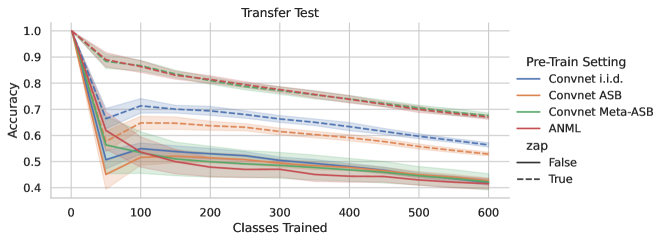
Figure 2: Performance in One-Layer Fine-Tuning on Omniglot. Removing the neuromodulation layers from ANML has no impact on performance (Meta-ASB and ANML both achieve 67% final accuracy). Removing zapping, however, drastically affects performance, even when employing meta-learning. We do not compare directly to OML since ANML represents the state of the art.

Compared to previous work our Meta-ASB setup doesn’t use heuristics on where/when in the model to apply optimization (like OML; Javed & White (2019)), nor context-dependent gating (like ANML; Beaulieu et al. (2020)), and uses fewer parameters than both prior works (see Appendix B). Despite the smaller architecture and simplified training regime used in our experiments, the continual learning performance is equal or better than both OML and ANML; see Figure 2 for a comparison against the ANML model in the setting where only One Layer is Fine-Tuned and the rest of the model is frozen (called OLFT in Beaulieu et al. (2020)). In the prior work, ANML achieved 63.8% accuracy after sequential learning of 600 classes. In our reimplementation, we show a slightly higher performance of 67% for both ANML and Meta-ASB.

This begs the question: if neither the separate optimization of inner-loop layers and outer-loop layers (as in both OML and ANML), nor neuromodulation (as in ANML) are necessary, then exactly what is it about these meta-learning algorithms that is contributing such drastic improvements? As we see from the solid green and red lines in Figure 2, the models trained without zapping—even though they were trained with meta-learning—show significantly lower performance (41.5% and 42.2% vs 67%).

In the following sections we will explore further how much both meta-learning and zapping contribute to classification performance in various settings. This is hinted at by the performance of Meta-ASB, ASB, and i.i.d. in Figure 2—zapping consistently improves all of them. However, for all further experiments we will focus on the “unfrozen” setting, where all layers are fine-tuned during transfer, as a better representative of continual learning.

3.2 Continual Learning

We evaluate the pre-trained variants described in 2.1.1 on the sequential transfer task as described in Section 2.1.2. To quickly recap, the entire models are fine-tuned (no weights are frozen) on a few examples from classes not seen during pre-training, the examples are shown one at a time, and an optimization step is taken after each one. In all datasets, the meta-learned models with zapping significantly outperform their non-zapping counterparts, and outperform i.i.d. pre-training by an additional margin (Figure 3).

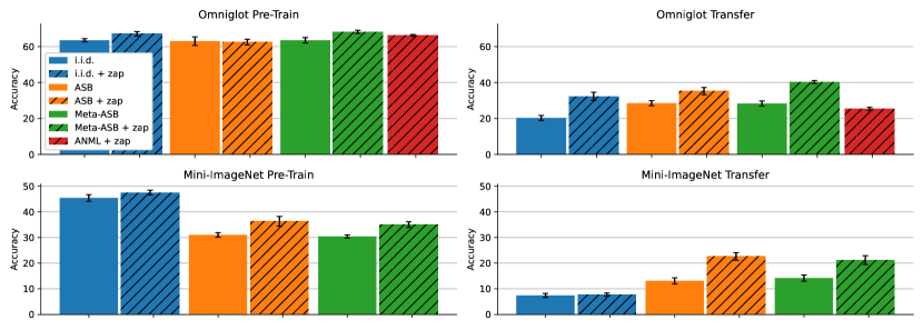
Figure 3: Average accuracy (and std dev error bars) for the unfrozen sequential transfer learning problem. Pre-Train is the final validation accuracy of the model on the pre-training dataset. Transfer is the accuracy on held-out instances from the transfer-to dataset at the very end of sequential fine-tuning (i.e. after training on all 600 or 20 classes). Models trained with zapping produce significantly better transfer accuracy than their counterparts without zapping in almost all cases. Additionally, our Convnet architecture improves substantially over the ANML method when all weights are unfrozen (red vs. green in the top right plot).

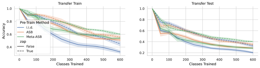
Figure 4: Accuracy on classes seen so far during sequential transfer learning on the Omniglot dataset. Left: Models are trained on a few (15) examples from 600 new classes not seen during pre-training. All 15 images from a class are shown sequentially one at a time before switching to the next class. Right: After each set of 50 classes (750 images), validation accuracy on the transfer set is measured using the remaining 5 examples from all classes seen up to that point. Models with zapping for all three pre-training methods (dashed lines) retain significantly more validation accuracy during and after the 600 classes (9000 updates), relative to models without zapping (solid lines).

On Omniglot (Figure 4), the best method with zapping achieves state-of-the-art transfer-and-finetune-all-layers validation accuracy of 40.3% after continual learning on a sequence of 9000 gradient updates (15 updates on each of 600 classes). The best model without zapping achieves only 28.5%. In fact, when applying zapping to i.i.d. pre-training, we can even achieve better performance (32.3%) than the models which are meta-learned without zapping (28.3%). This suggests that zapping may be an efficient and effective alternative (or complement) to higher-order gradients during pre-training.

On Mini-ImageNet (Figure 5), we again see a substantial difference between zapping models and their non-zapping counterparts (except for i.i.d.+zap). The same trends are more noticeable in the training accuracy, where the (zap ✔, meta ✔) model is able to retain nearly 100% of its training performance over 20 classes (600 image presentations), while the non-zapping models end up around 60%.

Figure 5: Accuracy on classes seen so far during continual transfer learning on Mini-ImageNet. Left: Models are trained on 30 examples from 20 new classes not seen during pre-training. All 30 images from a class are shown sequentially one at a time before switching to the next class. Right: After each class, validation accuracy on the transfer set is measured using 100 examples per class, from all classes seen up to that point. Models with zapping pre-trained with ASB (with or without meta-gradients) significantly outperform those configuration when trained without zapping. Models with i.i.d. pre-training show only transient improvements from zapping, achieving similar train and test accuracies at the end of these training sequences, and fail to reach the final accuracies found by any of the ASB methods.

In Figure 3, we also include the pre-train validation accuracy: this is the validation accuracy of the pre-trained model on the pre-training dataset, before it was modified for transfer. We observe that ranking models by validation performance is not well correlated with ranking of transfer performance. This lack of pre-training/transfer ranking correlation introduces a dilemma, whereby we may not have a reliable way of judging which models will be better for transfer until we actually try them.

Across all three datasets, we have observed that:

1. Zapping is a significant driver of performance improvements (see dashed vs. solid lines per treatment in Figures 2, 4, and 5).

2. Zapping sometimes also improves normal (pre-)training performance, although this trend is less consistent (Figure 3; more details in Tables 5 & 6 in the Appendix).

3. Counter-intuitively, even the Alternating Sequential and Batch learning (ASB) sampling routine alone (without meta-gradients) appears to provide some benefits for transfer (see ASB vs i.i.d. in Figure 5). It may sometimes be unnecessary to use the much more expensive and complex higher-order gradients.

3.3 Transfer Learning

Although the zapping and meta-learning methods described in Algorithm 1 were originally designed to learn robust representations for continual learning, we show that they are beneficial for transfer learning in general. Here we feature the results of standard i.i.d. transfer, as described in Section 2.1.2. We train each model for five epochs of unfrozen fine-tuning on mini-batches of data using the Adam optimizer.

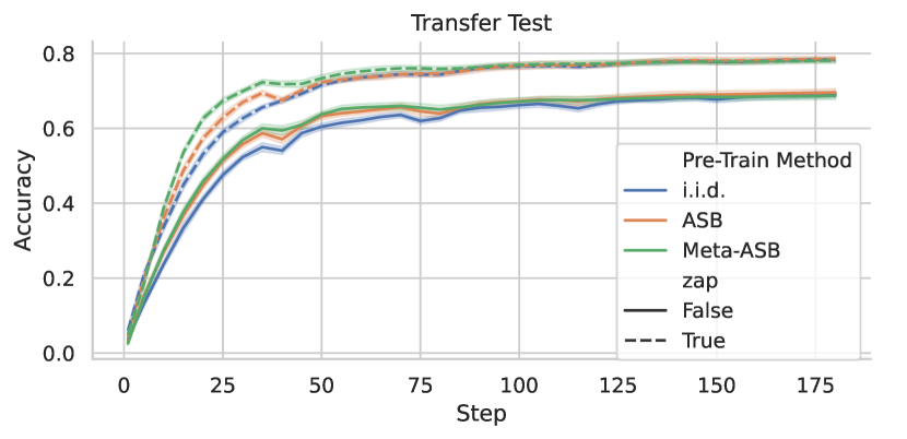
(a) Omniglot
(15 training images / 5 testing images per class).

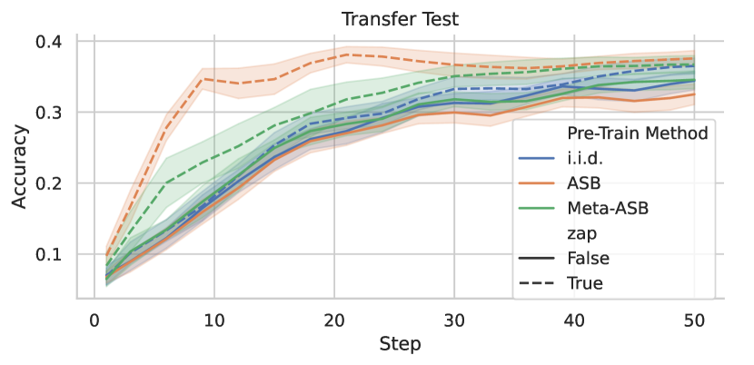
(b) Mini-ImageNet
(30 training / 100 testing images per class).

Figure 6: Validation accuracy over training time on all classes in the transfer set during fine-tuning with standard i.i.d. batches. For all datasets, models pre-trained with with zapping achieve significantly higher transfer accuracy at end of fine-tuning. While ASB methods (green, orange) do not dramatically improve final performance, they achieve more rapid fine-tuning relative to i.i.d. pre-training (blue).

Figure 6 shows results on Omniglot and Mini-ImageNet. As in the continual learning tests, here we also see substantial gains for the models employing zapping over those that do not. When zapping is not employed, models pre-trained with meta-gradients are comparable to those trained simply with standard i.i.d. pre-training. See Table 1 in Appendix A for a detailed comparison of final values.

Despite both the zapping and ASB pre-training methods stemming from attempts to reduce catastrophic forgetting in continual learning settings, zapping consistently provides advantages over non-zapped models for all pre-training configurations on standard i.i.d. transfer learning. We hypothesize that these two settings—continual and transfer learning—share key characteristics that make this possible. Both cases may benefit from an algorithm which produces more adaptable, robust features that can quickly learn new information while preserving prior patterns that may help in future tasks.

4 Discussion

Across three substantially different datasets (see Appendix F for the third dataset, OmnImage), zapping consistently results in better representations for transferring to few-shot datasets, leading to better performance in both a continual learning and standard transfer setting. In many cases, we are still able to achieve the best performance by just applying zapping and alternating optimizations of sequential learning and batch learning (ASB) without applying any meta-gradients.

We even see some benefit from applying zapping directly to i.i.d. training, without any sequential learning component. This raises the question of whether we can match the performance of meta-learning using only zapping and standard i.i.d. training. However, this setting introduces new choices of when and where to reset neurons, since we are learning in batches and not just one class at a time. We include ablations in Appendix H that examine this question; in most cases, more zapping leads to better performance, but it is still outmatched by ASB. However, more investigation of resetting schedules and heuristics will likely lead to discoveries of better hyperparameters.

It is reasonable to suppose that the constant injection of noise by resetting weights during training helps to discover weights which are not as affected by this disruption, thus building some resilience to the shock of re-initializing layers. If the improved performance can be attributed to noise injections reducing the co-adaptation of layers (Yosinski et al., 2014), thus increasing their resilience, it begs the question of how it relates to other co-adaptation reducing mechanisms such as dropout, which is also shown to improve continual (Mirzadeh et al., 2020) and transfer (Semwal et al., 2018) learning.

The approaches explored here include pre-training by alternating between sequential learning on a single class and batches sampled from all pre-training classes (ASB), and resetting classifier weights prior to training on a new class (zapping). The information accumulated by repeating these simple methods across many tasks during the pre-training process mimics the condition experienced during transfer learning at test time. We thus argue that the results above demonstrate a simple yet effective version of meta-learning—one without expensive meta-gradients to backpropagate through tasks.

5 Related work

As we have shown, the zapping operation of resetting last-layer weights provides clear performance improvements, but what about random weights enables this improved learning capability? The work of Frankle et al. (2020) investigates the dynamics of learning during the early stages of network training. They show that large gradients lead to substantial weight changes in the beginning of training, after which gradients and weight signs stabilize. Their work suggests that these initial drastic changes are linked to weight-level noise. Dohare et al. (2021) also investigate the relationship between noise and learning, showing that stochastic gradient descent is not enough to learn continually, and that this problem can be alleviated by repeated injections of noise. Rather than resetting classification neurons of the last layer, they choose weights to reset based on a pruning heuristic.

The reinitialization of weights in a neural network during training is an interesting emerging topic, with many other works investigating this phenomenon in a number of different settings. Like us, Zhao et al. (2018) periodically reinitialize the last layer of a neural network during training. Their focus is on ensemble learning for a single dataset, rather than transfer learning. Li et al. (2020) also periodically reinitialize the last layer, but they do it during transfer, rather than pre-training. Both Alabdulmohsin et al. (2021) and Zhou et al. (2022) investigated the idea of reinitialization of upper layers of the network, building upon the work of Taha et al. (2021). They show performance improvements in the few-shot regime. However, they they focus on learning of a single dataset rather than transfer learning. Zaidi et al. (2022) evaluate an extensive number of models to find under which circumstances reinitialization helps, although their work is also specific to training on a single dataset.

Nikishin et al. (2022) apply a similar mechanism to deep reinforcement learning. They find that periodically resetting the final layers of the Q-value network is beneficial across a broad array of settings. Some concurrent work (Ramkumar et al., 2023) study the application of resetting to a version of online learning where data arrives in mega-batches. They employ resetting as a compromise between fine-tuning a pre-trained network and training a new network from scratch.

One major difference between these prior works and our investigation is the zapping + ASB routine, where we forget one class at a time and focus on relearning that class. This meta-learning-like setting often achieves substantial gains beyond i.i.d.+zapping, and gives us a new lens through which to view weight resetting.

6 Conclusion & Future Work

We have revealed the importance of “zapping” for pre-training, and its connection to meta-learning. We have shown that zapping can lead to significant gains in transfer learning performance across multiple settings and datasets. The concept of forgetting and relearning has been investigated in other recent works, and our observations add to the growing evidence of the usefulness of this concept. We often see beneficial effects even without meta-learning or episodes of sequential learning, but the application of zapping to this setting is still relatively unexplored. Our work opens the door to further study and the discovery of ever more powerful uses of this zapping mechanism.

Aside from the benefits of zapping, our results highlight the disruptive effect of the re-initialization of last layers in general. Resetting of the final layer is routine in the process of fine-tuning a pre-trained model (Yosinski et al., 2014), but the impact of this “transfer shock” is still not fully clear. For instance, it was only recently observed that fine-tuning in this way underperforms on out-of-distribution examples, and Kumar et al. (2022) suggest to freeze the lower layers of a network to allow the final network to stabilize. A deeper understanding of these mechanisms could significantly benefit many areas of neural network research.

Finally, this work explores a simpler approach to meta-learning than meta-gradient approaches. It does so by repeatedly creating transfer shocks during pre-training, encouraging a network to learn to adapt to them. Future work should explore other methods by which we can approximate transfer learning during pre-training, how to influence the features learned to maximize transfer performance with the most computational efficiency, and how the benefits of zapping scale to larger models.

Appendix A Transfer Learning Scenarios

Pre-Train Method	Zap	Omniglot		Mini-ImageNet
		Pre-Train	Transfer	Pre-Train	Transfer
i.i.d.		63.5 $\pm 0.9$	69.0 $\pm 0.8$	45.4 $\pm 1.3$	34.4 $\pm 1.3$
i.i.d.	✔	67.1 $\pm 1.2$	78.4 $\pm 0.5$	47.5 $\pm 0.9$	36.5 $\pm 1.1$
ASB		63.0 $\pm 2.4$	69.6 $\pm 1.0$	43.9 $\pm 2.0$	32.5 $\pm 1.4$
ASB	✔	61.9 $\pm 1.2$	78.5 $\pm 0.8$	36.3 $\pm 1.9$	37.6 $\pm 1.1$
Meta-ASB		63.5 $\pm 1.5$	68.7 $\pm 1.0$	45.1 $\pm 1.3$	34.6 $\pm 1.2$
Meta-ASB	✔	68.2 $\pm 0.9$	77.8 $\pm 0.9$	17.1 $\pm 7.2$	36.7 $\pm 1.2$

Table 1: Average accuracy ($\pm$ std dev) for the standard fine-tuning transfer problem. Pre-Train is the final validation accuracy of the model on the pre-training dataset. Transfer is the accuracy on held-out instances from the transfer-to dataset after five epochs of fine-tuning. The best transfer configuration for each dataset (and those within one std dev) are highlighted in bold. Models trained with zapping produce significantly better transfer accuracy than those trained without zapping for all pre-training methods and datasets.

Here we describe our two transfer learning test cases from Section 2.1.2 in more formal detail. Algorithm 2 describes continual learning (results Section 3.2). Algorithm 3 describes i.i.d. learning (results Section 3.3). In both cases, the last layer of the pre-trained network is replaced with a new layer, and all layers are updated during the transfer process.

Algorithm 2 Sequential Transfer Protocol (adapted from Beaulieu et al. (2020), Algorithm 2)

1:$\mathcal{C}\leftarrow$ sequential trajectory of $N$ unseen classes

2:$\theta\leftarrow$ pre-trained weights of the network

3:$\beta\leftarrow$ learning rate hyperparameter

4:$S_{train}=[\ ]$

5:for $n=1,2,\ldots,N$ do

6:     $S_{traj}\sim\mathcal{C}_{n}$ $\triangleright$ get training examples from next class

7:     $S_{train}=S_{train}\bigcup S_{traj}$ $\triangleright$ add to sequential transfer train set

8:     for $i=1,2,\ldots,k$ do

9:         $\theta\leftarrow\theta-\beta\nabla_{\theta}\mathcal{L}(\theta,S^{(k)}_{traj})$ $\triangleright$ SGD update on a single image      

10:     record $\mathcal{L}(\theta,S_{train})$ $\triangleright$ eval current $\theta$ on classes trained so far

11:     $S_{test}=(\bigcup\limits_{1\ldots n}\mathcal{C}_{i})-S_{train}$ $\triangleright$ held-out examples from classes seen so far

12:     record $\mathcal{L}(\theta,S_{test})$ $\triangleright$ eval current $\theta$ on held-out examples

Algorithm 3 I.I.D. Transfer Protocol

1:$\mathcal{D}_{tr},\mathcal{D}_{te}\leftarrow$ training and held-out examples from $N$ unseen classes from domain $\mathcal{D}$

2:$\theta\leftarrow$ pre-trained weights of the network

3:$\beta\leftarrow$ learning rate hyperparameter

4:$E\leftarrow$ number of training epochs

5:for $i=1,2,\ldots,E$ do

6:     for $i=1,2,\ldots,N$ do $\triangleright$ $N$ is the number of batches in $\mathcal{D}_{tr}$

7:         $B_{i}\sim\mathcal{D}_{tr}$ $\triangleright$ uniformly sample next batch from domain $\mathcal{D}_{tr}$ without replacement

8:         $\theta\leftarrow\theta-\beta\nabla_{\theta}\mathcal{L}(\theta,\mathcal{B}_{i})$ $\triangleright$ standard batch SGD update

9:         record $\mathcal{L}(\theta,\mathcal{D}_{tr})$ $\triangleright$ eval current $\theta$ on all classes

10:         record $\mathcal{L}(\theta,\mathcal{D}_{te})$ $\triangleright$ eval current $\theta$ on all held-out examples      

Appendix B Separate Weights for Inner and Outer Loops

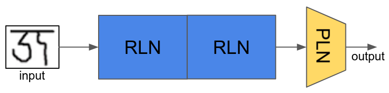
(a) OML architecture

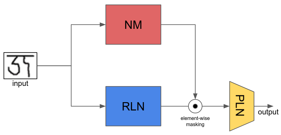
(b) ANML architecture

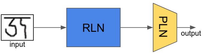
(c) Convnet architecture

Figure 7: OML, ANML and, Convnet architectures

As mentioned in Section 2, the meta-train phase is split between inner and outer loops. To incentivize the discovery of generalizable features the ANML and OML models train different parts of the model at different times. The last layer weights (pln in Figure 7(a)) are only updated in the inner loop while the whole network (rln + pln in Figure 7(a)) are updated only in the outer loop. The rationale of this choice is that the network can leverage meta-gradients in the outer loop to find features that can improve the inner loop.

In a similar fashion the ANML model only updates the neuromodulation weights (NM in Figure 7(b)) using meta-gradients in the outer loop, while instead the rest of the weights (rln + pln in Figure 7(b)). This design choice aims to break the symmetry of inner/outer loops and incentivize the outer loop to refine/integrate what was learned during the inner loop. See Table 2 for a comparison of the various methods.

	Inner (SGD)			Outer (meta-Adam)
	NM	RLN	PLN	NM	RLN	PLN
OML	-	✕	✔	-	✔	✔
ANML	✕	✔	✔	✔	✔	✔
Convnet	-	✔	✔	-	✔	✔

Table 2: Different update strategies

Unlike ANML and OML, our Convnet updates all weights in every phase. We remove the NM layers from the ANML model, yet perform just as well in one-layer fine-tuning (Figure 2) or better in unfrozen transfer (Figure 8). Our architecture is also shallower than OML (3 conv layers instead of 6).

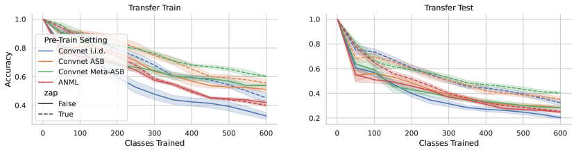
Figure 8: Accuracy on continual learning of Omniglot; this is the same as Figure 4, but we add the ANML method for comparison. We can see that ANML suffers from much more catastrophic forgetting than Convnet does.

Appendix C Hyperparameters

We use the Adam optimizer (Kingma & Ba, 2014) with a standard cross-entropy loss. We train all models to convergence on all our datasets, and we take the final checkpoint as our pre-trained model for continual/transfer tests. In the i.i.d. pre-training setting, we do not have the single-class inner loop, so we must decide how often to zap in a different manner. We investigate the effect of zapping at different frequencies and a different number of classes (from a single one to all of them at once) to determine the optimal configuration (Appendix H).

See Tables 3 and 4 for a listing of pre-training hyperparameters used for our experiments.

Parameter	Omniglot / OmnImage	Mini-ImageNet
training examples per class	15	500
validation examples per class	5	100
inner loop steps	20	same
“remember set” size	64	100
inner optimizer	SGD	same
inner learning rates	[0.1, 0.01, 0.001]	same
outer optimizer	Adam	same
outer learning rates	[0.1, 0.01, 0.001]	same
outer loop steps	9,000	same

Table 3: Hyperparameters used for pre-training using Alternating Sequential and Batch Learning (ASB).

Parameter	Omniglot / OmnImage	Mini-ImageNet
training examples per class	15	500
validation examples per class	5	100
Adam learning rates	[3e-4, 1e-3, 3e-4]	same
batch size	256	same
epochs	10 / 30	30

Table 4: Hyperparameters used for pre-training using standard i.i.d. batch learning.

Appendix D Network Architecture

See Figure 9 for a depiction of the neural network architecture used in this work. The Mini-ImageNet and OmnImage datasets consist of images of size 84x84. For these, we use a typical architecture consisting of four convolutional blocks and one fully-connected final layer. Each convolutional block consists of: convolution, InstanceNorm (Ulyanov et al., 2016), ReLU activation, and max pool layers, in that order. All convolutional layers have 256 output channels. An architecture similar to this has been used to good effect for much exploratory research in few-shot learning—in particular, we were inspired by “Few-Shot Meta-Baseline” (Chen et al., 2021).

For Omniglot, we use 28x28 single-channel images, and so the architecture is slightly different. Instead of four convolutional blocks, we use three. Also, we skip the final pooling layer.

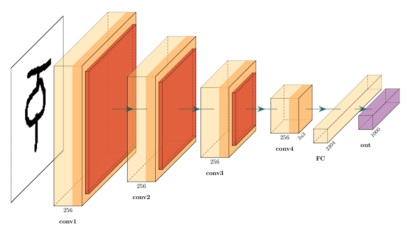
Figure 9: Convnet4, a standard architecture with four convolutional blocks and one fully-connected linear layer. The example in this case corresponds to a hypothetical dataset which has 1,000 target classes.

Appendix E Alternating Sequential and Batch Learning

See Figure 10 for a visual depiction of the Alternating Sequential and Batch (ASB) learning procedure, and its meta-learning variant.

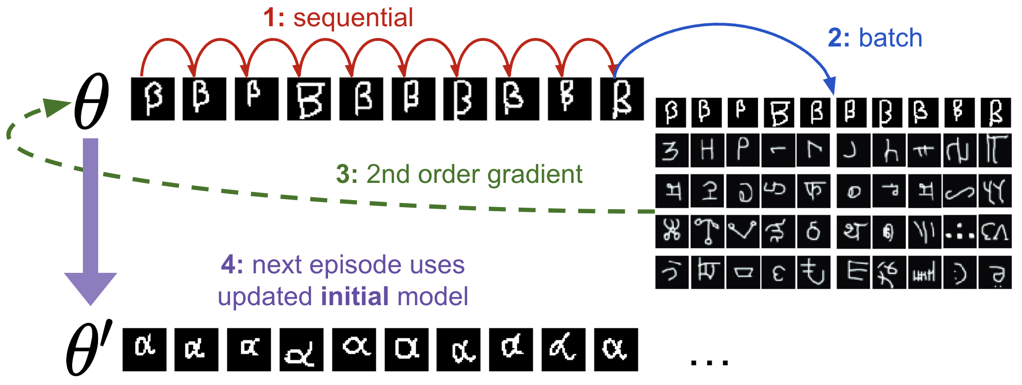
(a) Meta-ASB

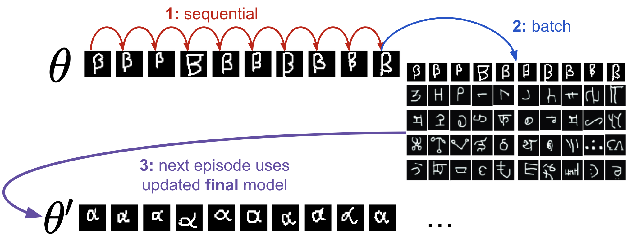
(b) ASB

Figure 10: The ASB training procedure with and without higher-order gradients based meta-learning.

Appendix F OmnImage Dataset

While Mini-ImageNet contains more challenging imagery, it has far fewer classes than Omniglot, and thus cannot form a very long continual learning trajectory. To better test the effect of zapping in a continual learning setting that uses natural images, we test our models on a different subset of ImageNet with a shape similar to Omniglot (1000 classes, 20 images per class), called OmnImage (Frati et al., 2023). Similarly to the Omniglot case where each class contains very similar characters, the classes in OmnImage are selected to maximize within-class consistency by selecting the 20 most similar images per class via an evolutionary algorithm. See Appendix F.1, Figure 11 for a visual comparison of the datasets used, highlighting the similarity between Omniglot and OmnImage, and see Frati et al. (2023), for full details of the dataset.

F.1 Dataset Comparison

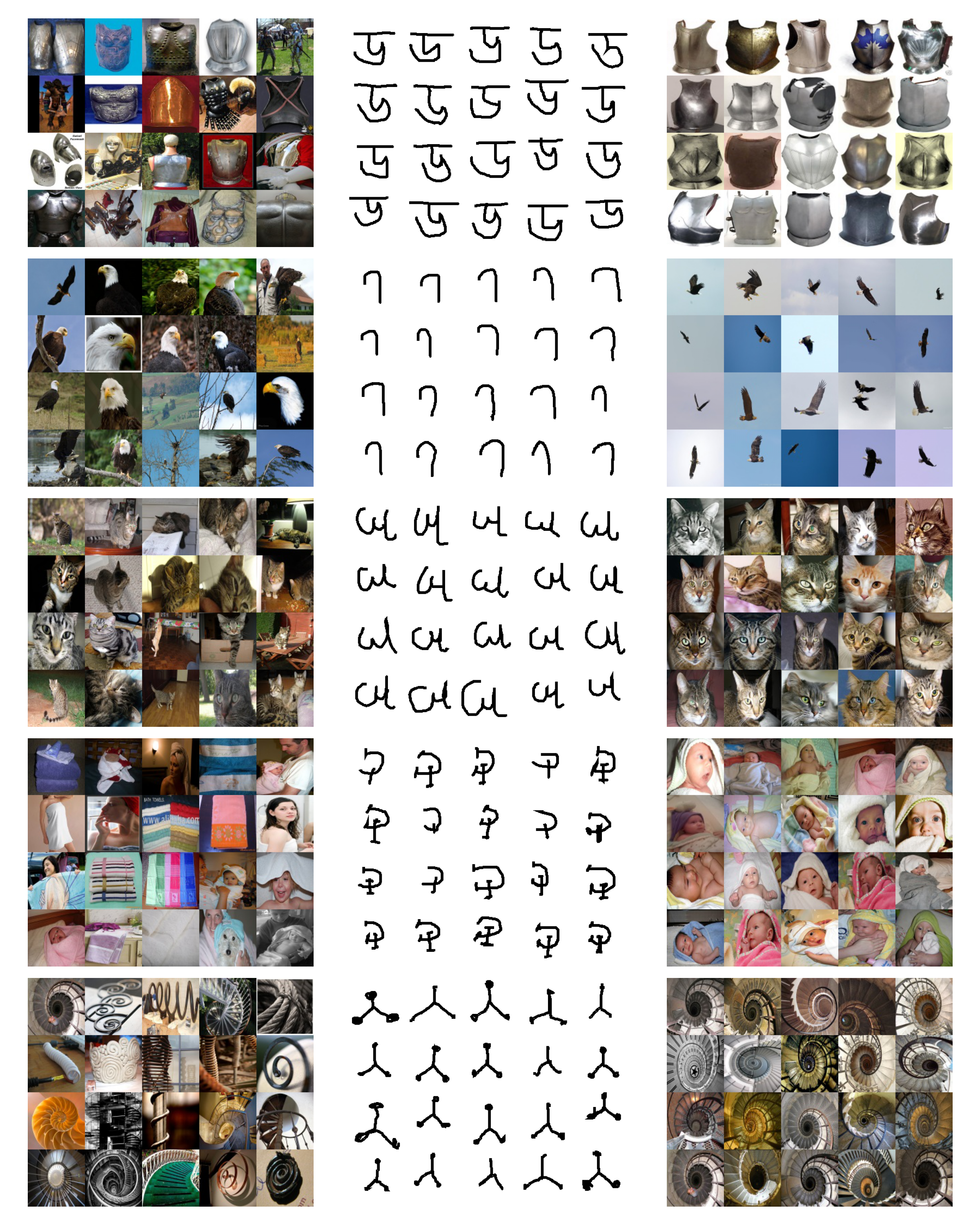
Figure 11: Comparing Mini-ImageNet, Omniglot and OmnImage: Samples drawn from the Mini-Image dataset (left column) are both more complex and more visually varied than the simple and consistent one from Omniglot (center column). On the other hand, images from OmnImage (right column) are selected for visual similarity and more closely resemble the many classes with few-consistent examples structure of Omniglot.

F.2 Continual Learning

The OmnImage dataset represents a difficult continual learning problem, since it consists of a long trajectory of complex natural images (300 test classes, 6000 total training images). Although all configurations struggle to achieve good accuracy on OmnImage, we see elevated transfer performance for zapping configurations (Figure 12(b)). Note that Figure 12 shows results when all the weights are updated during continual learning, like ANML-unlimited setting from Beaulieu et al. (2020).

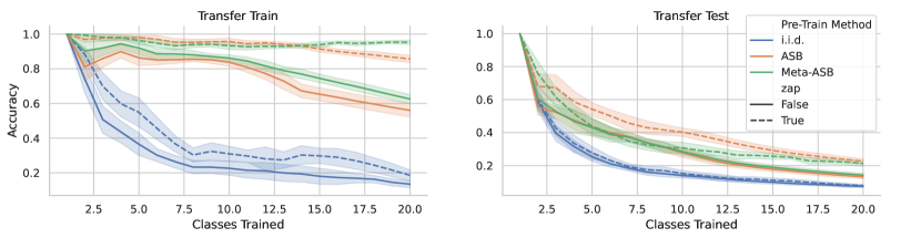
(a) Mini-ImageNet, trained on 30 images per class.

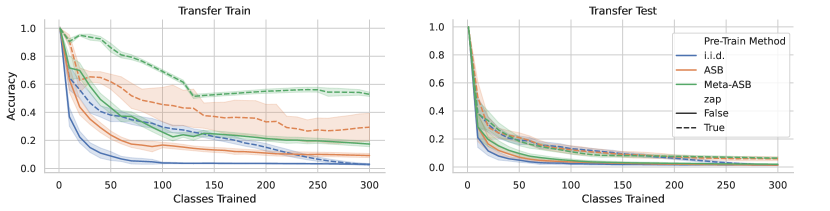
(b) OmnImage, trained on 15 images per class.

Figure 12: Accuracy on classes seen so far during continual transfer learning on Mini-ImageNet (top) and OmnImage (bottom). Left is training accuracy on examples seen during transfer learning (but from classes not seen during pre-training). Right is validation accuracy on held-out examples from the transfer dataset. Models with zapping pre-trained on ASB data (with or without meta-gradients) significantly outperform those configuration when trained without zapping. Models with i.i.d. pre-training show only transient improvements from zapping, achieving similar train and test accuracies at the end of these training sequences, and fail to reach the final accuracies found by any of the ASB methods (irrespective of their use of meta-gradients or zapping).

Pre-Train Method	Zap	Omniglot		Mini-ImageNet		OmnImage
		Pre-Train	Transfer	Pre-Train	Transfer	Pre-Train	Transfer
i.i.d.		63.5 $\pm 0.9$	20.3 $\pm 1.4$	45.4 $\pm 1.3$	7.4 $\pm 0.8$	19.7 $\pm 0.6$	1.4 $\pm 0.3$
i.i.d.	✔	67.1 $\pm 1.2$	32.3 $\pm 2.3$	47.5 $\pm 0.9$	7.8 $\pm 0.6$	26.8 $\pm 2.1$	1.4 $\pm 0.4$
ASB		63.0 $\pm 2.4$	28.5 $\pm 1.4$	31.0 $\pm 0.9$	13.1 $\pm 1.2$	7.5 $\pm 0.7$	1.4 $\pm 0.3$
ASB	✔	62.5 $\pm 1.6$	35.2 $\pm 2.0$	36.3 $\pm 1.9$	22.6 $\pm 1.5$	20.9 $\pm 1.3$	5.9 $\pm 1.3$
Meta-ASB		63.5 $\pm 1.5$	28.3 $\pm 1.4$	30.4 $\pm 0.6$	14.2 $\pm 1.2$	6.8 $\pm 0.8$	2.0 $\pm 0.4$
Meta-ASB	✔	68.2 $\pm 0.9$	40.3 $\pm 0.8$	35.0 $\pm 1.1$	21.2 $\pm 1.7$	11.4 $\pm 1.9$	6.3 $\pm 0.6$
ANML-Unlimited	✔	66.2 $\pm 0.5$	25.3 $\pm 0.9$	-	-	-	-

Table 5: Average accuracy ($\pm$ std dev) for the unfrozen sequential transfer learning problem. Pre-Train is the final validation accuracy of the model on the pre-training dataset. Transfer is the accuracy on held-out instances from the transfer-to dataset at the very end of sequential fine-tuning (i.e. after training on all 600/20/300 classes). The best transfer configuration for each dataset (and those within one std dev) are highlighted in bold. Models trained with zapping produce better transfer accuracy than their counterparts without zapping in almost all cases. Additionally, our Convnet architecture improves substantially over the ANML method when all weights are unfrozen.

F.3 Transfer Learning

The effect of {Meta-}ASB on OmnImage is particularly striking (Figure 13) when performing standard transfer learning. The best testing performance with zapping (30.5%) is almost double the performance of standard i.i.d. pre-training (16.3%), after 5 epochs, and more importantly each zapping treatment outperforms their no-zapping counterparts (see Figures 6 & 13).

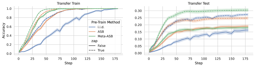
Figure 13: Training (left) and test (right) accuracy on classes during standard fine-tuning on the OmnImage subset of ImageNet (15 training images / 5 test images per class). Models pre-trained with zapping achieve significantly higher test accuracies, with models employing both meta-gradients and zapping coming out on top.

Pre-Train Method	Zap	Omniglot		Mini-ImageNet		OmnImage
		Pre-Train	Transfer	Pre-Train	Transfer	Pre-Train	Transfer
i.i.d.		63.5 $\pm 0.9$	69.0 $\pm 0.8$	45.4 $\pm 1.3$	34.4 $\pm 1.3$	27.2 $\pm 0.5$	16.3 $\pm 1.2$
i.i.d.	✔	67.1 $\pm 1.2$	78.4 $\pm 0.5$	47.5 $\pm 0.9$	36.5 $\pm 1.1$	26.8 $\pm 2.1$	27.3 $\pm 0.8$
ASB		63.0 $\pm 2.4$	69.6 $\pm 1.0$	43.9 $\pm 2.0$	32.5 $\pm 1.4$	18.6 $\pm 0.3$	19.1 $\pm 0.9$
ASB	✔	61.9 $\pm 1.2$	78.5 $\pm 0.8$	36.3 $\pm 1.9$	37.6 $\pm 1.1$	20.9 $\pm 1.3$	24.8 $\pm 0.9$
Meta-ASB		63.5 $\pm 1.5$	68.7 $\pm 1.0$	45.1 $\pm 1.3$	34.6 $\pm 1.2$	22.0 $\pm 1.0$	18.0 $\pm 0.9$
Meta-ASB	✔	68.2 $\pm 0.9$	77.8 $\pm 0.9$	17.1 $\pm 7.2$	36.7 $\pm 1.2$	28.9 $\pm 0.7$	30.5 $\pm 1.1$

Table 6: Average accuracy ($\pm$ std dev) for the standard fine-tuning transfer problem. Pre-Train is the final validation accuracy of the model on the pre-training dataset. Transfer is the accuracy on held-out instances from the transfer-to dataset after five epochs of fine-tuning. The best transfer configuration for each dataset (and those within one std dev) are highlighted in bold. Models trained with zapping produce significantly better transfer accuracy than those trained without zapping for all pre-training methods and datasets.

Appendix G Cross-Domain Transfer

In the main text, we pre-train on a subset of classes from a dataset, and transfer to a unique disjoint subset of classes on the same dataset. But the typical use case for a pre-trained model is to transfer to a different dataset—potentially even a significantly different domain. Here we test whether zapping provides benefits when transferring across datasets. We find that it does slightly boost performance in this setting, but the results or more mixed and more investigation is warranted.

Figures 14 shows cross-domain i.i.d. transfer onto the Omniglot dataset, using models which were pre-trained on other datasets. We can see that, while the non-zapping models do catch up with sufficient training epochs, all the zapping models adapt to the new domain faster (all dashed lines are above their corresponding solid lines).

Figure 15 instead shows the results of sequential transfer (i.e. training on a single image at a time). Zapping does help transfer from OmnImage to Omniglot, but not from Mini-Imagenet. In general, OmnImage seems to benefit most from zapping, both within-domain and across domains. We see this again in transferring OmnImage to Mini-ImageNet, shown in Figure 16.

Thus we see that models with zapping are often capable of faster adaptation in transferring to a new domain, and sometimes exhibit better final performance as well. However, by comparison to Figure 3 and 1, we can see that it is still generally beneficial to pre-train on a domain which is similar to the transferred domain, when possible. Zapping can help improve performance of a given pre-training setting, but it does not fully overcome the effects of a large distribution shift.

(a) Transfer from Mini-ImageNet to Omniglot.

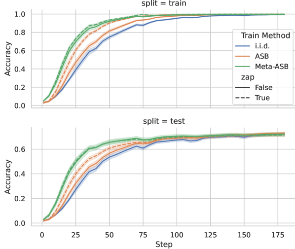
(b) Transfer from OmnImage to Omniglot.

Figure 14: Cross-domain transfer onto the Omniglot dataset, using five epochs of standard fine-tuning.

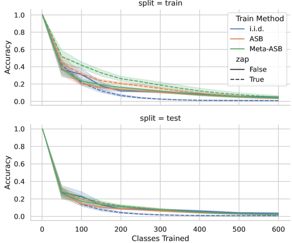
(a) Sequential transfer from Mini-ImageNet to Omniglot.

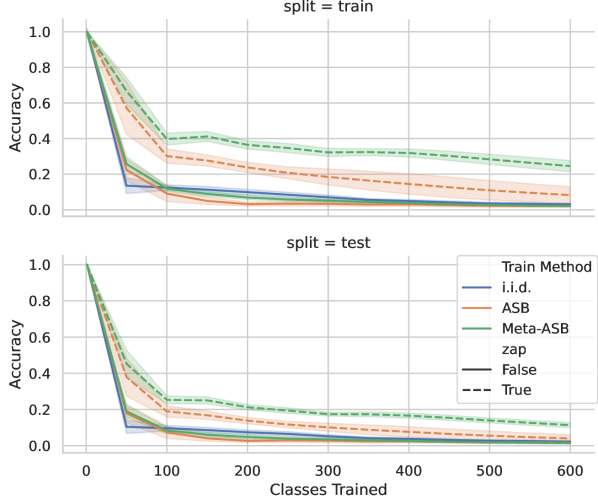
(b) Sequential transfer from OmnImage to Omniglot.

Figure 15: Cross-domain sequential transfer onto the Omniglot dataset; training on a sequence of 600 classes, 15 images per class.

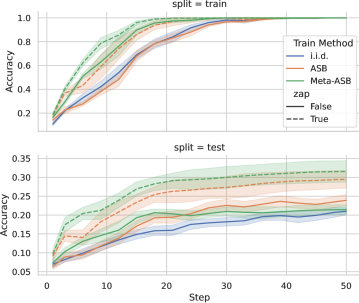
Figure 16: Transfer from OmnImage to Mini-ImageNet, using five epochs of standard fine-tuning.

Appendix H Performing Zapping in i.i.d. Pre-Training

During ASB, the model is presented with episodes of sequential learning on a single class, so we always reset the last layer weights corresponding to the class which is about to undergo sequential learning. In the i.i.d. case, there is no such "single task training phase". Instead, we choose to reset $K$ classes (out of $N$ total classes) on a cadence of once per $E$ epochs. This introduces two new hyperparameters $(K,E)$ for us to sweep over.

Here we show results for all three datasets attempting different numbers of neurons for resets (differing values of $K$). We also tried resetting less often than once per epoch ($E>1$), but resetting every epoch was typically better. In fact, in most cases below, the best scenario is to reset all last layer weights at the beginning of every epoch. Fine-tuning trajectories are shown in Figures 17, 18, and 19; and final performance is summarized in Tables 7 and 8.

These experiments show the potential for applying zapping to standard batch gradient descent. Our variants with more zapping generally see improved transfer, even though the effect is not as substantial as when it is paired with ASB. It stands to reason that there should be some point at which too much resetting becomes detrimental, and we have not tried to reset more often than once per epoch ($E<1$) in the i.i.d. setting, so this would be a great starting point for future work.

Zap Amount	Omniglot		Mini-ImageNet		OmnImage
	Valid	Transfer	Valid	Transfer	Valid	Transfer
none	63.5 $\pm 0.9$	20.3 $\pm 1.4$	45.4 $\pm 1.3$	7.4 $\pm 0.8$	27.2 $\pm 0.5$	1.4 $\pm 0.4$
small	63.2 $\pm 1.5$	23.5 $\pm 2.5$	44.8 $\pm 1.0$	7.9 $\pm 1.0$	21.2 $\pm 0.5$	1.1 $\pm 0.4$
medium	66.3 $\pm 1.2$	21.5 $\pm 6.6$	47.3 $\pm 1.0$	7.8 $\pm 0.7$	24.4 $\pm 0.9$	1.3 $\pm 0.3$
large	66.7 $\pm 1.1$	22.0 $\pm 6.5$	47.5 $\pm 0.3$	7.3 $\pm 0.8$	29.0 $\pm 0.7$	2.1 $\pm 0.6$
all	67.1 $\pm 1.2$	32.3 $\pm 2.3$	47.5 $\pm 0.9$	7.7 $\pm 0.9$	26.8 $\pm 2.1$	1.4 $\pm 0.4$

Table 7: Accuracy for unfrozen sequential transfer on i.i.d. pre-trained models with different amounts of zapping. Results are aggregated in the same way as the tables in the main text.

Zap Amount	Omniglot		Mini-ImageNet		OmnImage
	Valid	Transfer	Valid	Transfer	Valid	Transfer
none	63.5 $\pm 0.9$	69.0 $\pm 0.8$	45.4 $\pm 1.3$	34.4 $\pm 1.3$	27.2 $\pm 0.5$	16.3 $\pm 1.2$
small	63.2 $\pm 1.5$	71.3 $\pm 0.7$	44.8 $\pm 1.0$	35.2 $\pm 1.1$	21.2 $\pm 0.5$	22.7 $\pm 0.8$
medium	66.3 $\pm 1.2$	75.4 $\pm 0.7$	47.3 $\pm 1.0$	35.7 $\pm 1.2$	24.4 $\pm 0.9$	24.6 $\pm 1.1$
large	66.7 $\pm 1.1$	77.1 $\pm 0.7$	47.5 $\pm 0.3$	36.1 $\pm 0.8$	29.0 $\pm 0.7$	27.5 $\pm 1.0$
all	67.1 $\pm 1.2$	78.3 $\pm 0.4$	47.5 $\pm 0.9$	36.5 $\pm 1.1$	26.8 $\pm 2.1$	27.3 $\pm 0.8$

Table 8: Accuracy for standard fine-tuning on i.i.d. pre-trained models with different amounts of zapping. Results are aggregated in the same way as the tables in the main text.

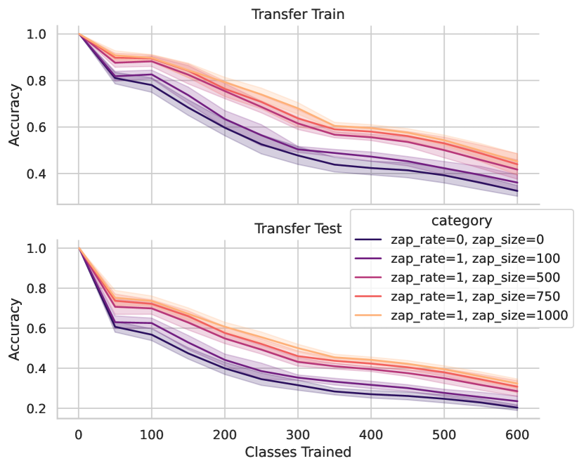
(a) Omniglot Sequential Transfer.

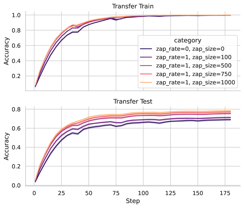
(b) Omniglot i.i.d. Transfer.

Figure 17: The effect of applying different amounts of zapping to standard i.i.d. models, pre-trained on Omniglot.

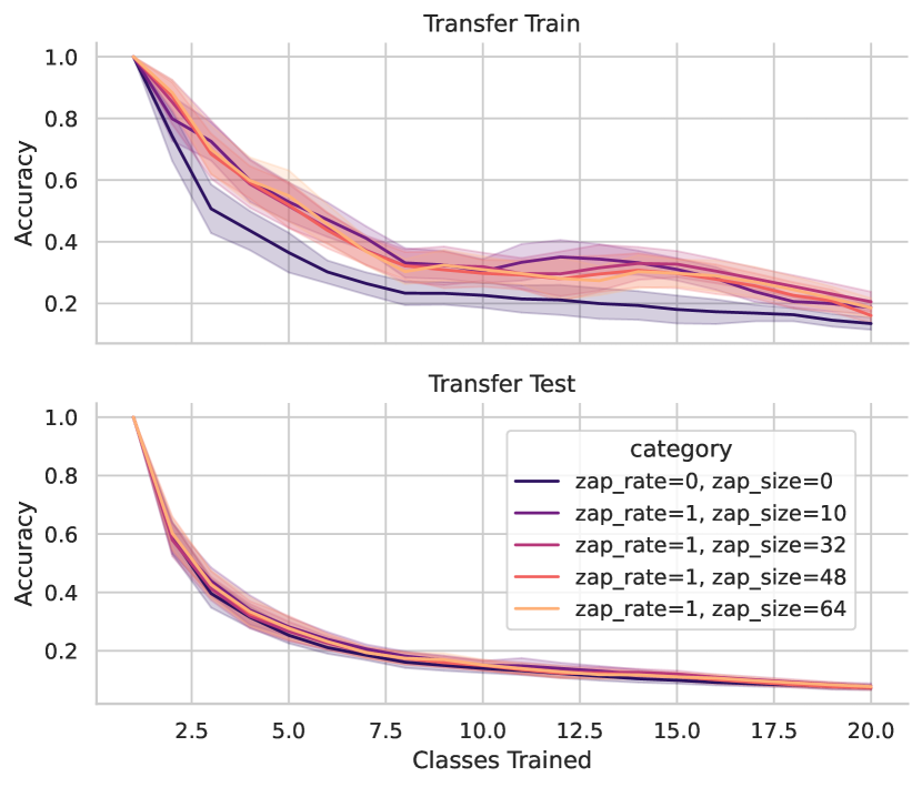
(a) Mini-ImageNet Sequential Transfer.

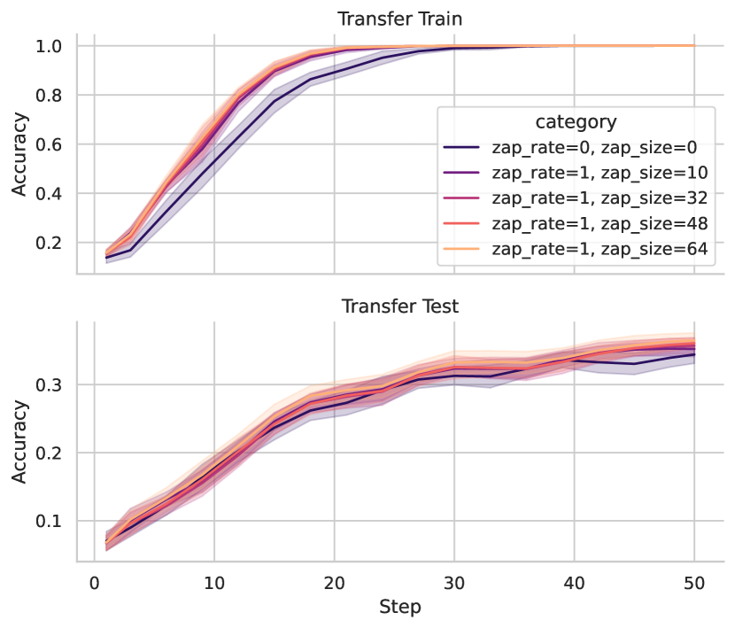
(b) Mini-ImageNet i.i.d. Transfer.

Figure 18: The effect of applying different amounts of zapping to standard i.i.d. models, pre-trained on Mini-ImageNet.

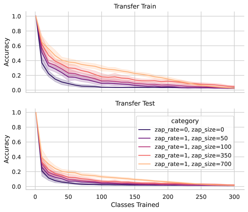
(a) OmnImage Sequential Transfer.

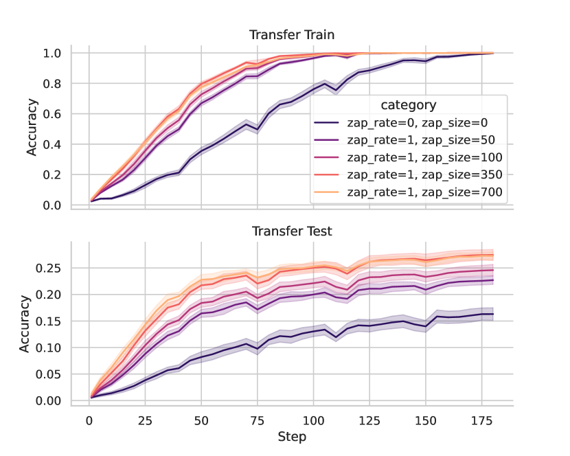
(b) OmnImage i.i.d. Transfer.

Figure 19: The effect of applying different amounts of zapping to standard i.i.d. models, pre-trained on OmnImage.

References

- Alabdulmohsin et al. (2021) Ibrahim Alabdulmohsin, Hartmut Maennel, and Daniel Keysers. The impact of reinitialization on generalization in convolutional neural networks. arXiv preprint arXiv:2109.00267, 2021.
- Beaulieu et al. (2020) Shawn Beaulieu, Lapo Frati, Thomas Miconi, Joel Lehman, Kenneth O Stanley, Jeff Clune, and Nick Cheney. Learning to continually learn. arXiv preprint arXiv:2002.09571, 2020.
- Bengio et al. (1990) Yoshua Bengio, Samy Bengio, and Jocelyn Cloutier. Learning a synaptic learning rule. Citeseer, 1990.
- Chen et al. (2021) Yinbo Chen, Zhuang Liu, Huijuan Xu, Trevor Darrell, and Xiaolong Wang. Meta-baseline: Exploring simple meta-learning for few-shot learning. In Proceedings of the IEEE/CVF International Conference on Computer Vision, pp. 9062–9071, 2021.
- Dohare et al. (2021) Shibhansh Dohare, A Rupam Mahmood, and Richard S Sutton. Continual backprop: Stochastic gradient descent with persistent randomness. arXiv preprint arXiv:2108.06325, 2021.
- Félix & Wagner (2008) Marie-Anne Félix and Andreas Wagner. Robustness and evolution: concepts, insights and challenges from a developmental model system. Heredity, 100(2):132–140, 2008.
- Fernando et al. (2018) Chrisantha Fernando, Jakub Sygnowski, Simon Osindero, Jane Wang, Tom Schaul, Denis Teplyashin, Pablo Sprechmann, Alexander Pritzel, and Andrei Rusu. Meta-learning by the baldwin effect. In Proceedings of the Genetic and Evolutionary Computation Conference Companion, pp. 1313–1320, 2018.
- Finn et al. (2017) Chelsea Finn, Pieter Abbeel, and Sergey Levine. Model-agnostic meta-learning for fast adaptation of deep networks. In International Conference on Machine Learning, pp. 1126–1135. PMLR, 2017.
- Frankle et al. (2020) Jonathan Frankle, David J Schwab, and Ari S Morcos. The early phase of neural network training. arXiv preprint arXiv:2002.10365, 2020.
- Frati et al. (2023) Lapo Frati, Neil Traft, and Nick Cheney. Omnimage: Evolving 1k image cliques for few-shot learning. In Proceedings of the Genetic and Evolutionary Computation Conference, GECCO ’23, New York, NY, USA, 2023. Association for Computing Machinery.
- He et al. (2015) Kaiming He, Xiangyu Zhang, Shaoqing Ren, and Jian Sun. Delving deep into rectifiers: Surpassing human-level performance on imagenet classification. In Proceedings of the IEEE international conference on computer vision, pp. 1026–1034, 2015.
- Hochreiter et al. (2001) Sepp Hochreiter, A Steven Younger, and Peter R Conwell. Learning to learn using gradient descent. In Artificial Neural Networks—ICANN 2001: International Conference Vienna, Austria, August 21–25, 2001 Proceedings 11, pp. 87–94. Springer, 2001.
- Hoffer et al. (2018) Elad Hoffer, Itay Hubara, and Daniel Soudry. Fix your classifier: The marginal value of training the last weight layer. arXiv preprint arXiv:1801.04540, 2018.
- Javed & White (2019) Khurram Javed and Martha White. Meta-learning representations for continual learning. arXiv preprint arXiv:1905.12588, 2019.
- Kingma & Ba (2014) Diederik P Kingma and Jimmy Ba. Adam: A method for stochastic optimization. arXiv preprint arXiv:1412.6980, 2014.
- Kumar et al. (2022) Ananya Kumar, Aditi Raghunathan, Robbie Matthew Jones, Tengyu Ma, and Percy Liang. Fine-tuning can distort pretrained features and underperform out-of-distribution. In International Conference on Learning Representations, 2022. URL https://openreview.net/forum?id=UYneFzXSJWh.
- Lake et al. (2015) Brenden M Lake, Ruslan Salakhutdinov, and Joshua B Tenenbaum. Human-level concept learning through probabilistic program induction. Science, 350(6266):1332–1338, 2015.
- Li et al. (2020) Xingjian Li, Haoyi Xiong, Haozhe An, Cheng-Zhong Xu, and Dejing Dou. Rifle: Backpropagation in depth for deep transfer learning through re-initializing the fully-connected layer. In International Conference on Machine Learning, pp. 6010–6019. PMLR, 2020.
- Mirzadeh et al. (2020) Seyed Iman Mirzadeh, Mehrdad Farajtabar, and Hassan Ghasemzadeh. Dropout as an implicit gating mechanism for continual learning. In Proceedings of the IEEE/CVF Conference on Computer Vision and Pattern Recognition Workshops, pp. 232–233, 2020.
- Nikishin et al. (2022) Evgenii Nikishin, Max Schwarzer, Pierluca D’Oro, Pierre-Luc Bacon, and Aaron Courville. The primacy bias in deep reinforcement learning. In International Conference on Machine Learning, pp. 16828–16847. PMLR, 2022.
- Ramkumar et al. (2023) Vijaya Raghavan T Ramkumar, Elahe Arani, and Bahram Zonooz. Learn, unlearn and relearn: An online learning paradigm for deep neural networks. Transactions on Machine Learning Research, 2023. ISSN 2835-8856. URL https://openreview.net/forum?id=WN1O2MJDST.
- Ravi & Larochelle (2017) Sachin Ravi and Hugo Larochelle. Optimization as a model for few-shot learning. In International conference on learning representations, 2017.
- Rohlf & Winkler (2009) Thimo Rohlf and Christopher R Winkler. Emergent network structure, evolvable robustness, and nonlinear effects of point mutations in an artificial genome model. Advances in Complex Systems, 12(03):293–310, 2009.
- Schmidhuber (1987) Jürgen Schmidhuber. Evolutionary principles in self-referential learning, or on learning how to learn: the meta-meta-… hook. PhD thesis, Technische Universität München, 1987.
- Semwal et al. (2018) Tushar Semwal, Promod Yenigalla, Gaurav Mathur, and Shivashankar B Nair. A practitioners’ guide to transfer learning for text classification using convolutional neural networks. In Proceedings of the 2018 SIAM international conference on data mining, pp. 513–521. SIAM, 2018.
- Taha et al. (2021) Ahmed Taha, Abhinav Shrivastava, and Larry S Davis. Knowledge evolution in neural networks. In Proceedings of the IEEE/CVF Conference on Computer Vision and Pattern Recognition, pp. 12843–12852, 2021.
- Ulyanov et al. (2016) Dmitry Ulyanov, Andrea Vedaldi, and Victor Lempitsky. Instance normalization: The missing ingredient for fast stylization. arXiv preprint arXiv:1607.08022, 2016.
- Vinyals et al. (2016) Oriol Vinyals, Charles Blundell, Timothy Lillicrap, Daan Wierstra, et al. Matching networks for one shot learning. Advances in neural information processing systems, 29:3630–3638, 2016.
- Yosinski et al. (2014) Jason Yosinski, Jeff Clune, Yoshua Bengio, and Hod Lipson. How transferable are features in deep neural networks? Advances in neural information processing systems, 27, 2014.
- Zaidi et al. (2022) Sheheryar Zaidi, Tudor Berariu, Hyunjik Kim, Jörg Bornschein, Claudia Clopath, Yee Whye Teh, and Razvan Pascanu. When does re-initialization work? arXiv preprint arXiv:2206.10011, 2022.
- Zhao et al. (2018) Kaikai Zhao, Tetsu Matsukawa, and Einoshin Suzuki. Retraining: A simple way to improve the ensemble accuracy of deep neural networks for image classification. In 2018 24th International Conference on Pattern Recognition (ICPR), pp. 860–867. IEEE, 2018.
- Zhou et al. (2022) Hattie Zhou, Ankit Vani, Hugo Larochelle, and Aaron Courville. Fortuitous forgetting in connectionist networks. In International Conference on Learning Representations, 2022. URL https://openreview.net/forum?id=ei3SY1_zYsE.