KEK-TH-2557
Effective Brane Field Theory with
Higher-form Symmetry

Abstract

We propose an effective field theory for branes with higher-form symmetry as a generalization of ordinary Landau theory, which is an extension of the previous work by Iqbal and McGreevy for one-dimensional objects to an effective theory for $p$-dimensional objects. In the case of a $p$-form symmetry, the fundamental field $\psi[C_{p}]$ is a functional of $p$-dimensional closed brane $C_{p}$ embedded in a spacetime. As a natural generalization of ordinary field theory, we call this theory the brane field theory. In order to construct an action that is invariant under higher-form transformation, we generalize the idea of area derivative for one-dimensional objects to higher-dimensional ones. Following this, we discuss various fundamental properties of the brane field based on the higher-form invariant action. It is shown that the classical solution exhibits the area law in the unbroken phase of $\mathrm{U}(1)$ $p$-form symmetry, while it indicates a constant behavior in the broken phase for the large volume limit of $C_{p}$. In the latter case, the low-energy effective theory is described by the $p$-form Maxwell theory. We also discuss brane-field theories with a discrete higher-form symmetry and show that the low-energy effective theory becomes a BF-type topological field theory, resulting in topological order. Finally, we present a concrete brane-field model that describes a superconductor from the point of view of higher-form symmetry.

1 Introduction

Symmetry is one of the most important and fundamental concepts in modern physics, and it plays an essential role in classifying phases of vacuum and matter. For instance, various phase transitions can be comprehended through the presence of symmetries and their spontaneous breaking. The Landau theory provides a comprehensive and effective framework for this description [1, 2]. In the Landau theory and its extensions, an order parameter field $\phi(X)$, charged under a global symmetry, is introduced, and the theory (i.e., free energy, Hamiltonian, or Lagrangian) is constructed as invariant under the symmetry. Furthermore, it is important to note that the assumption of the conventional Landau theory is that the order parameter $\phi(X)$ is a local function of the spacetime point. In this sense, the conventional Landau theory describes an effective theory of point-like or zero-dimensional objects, such as particles.

The concept of symmetry has been recently extended in various directions, called “generalized global symmetries” [3], which include higher-form [4, 5, 6, 7, 8, 9, 10, 11, 12, 13, 14], higher-group [15, 16, 17, 18, 19, 20, 21, 22, 23, 24, 25, 26, 27, 28, 29, 30, 31], and noninvertible symmetries [32, 33, 34, 35, 36, 37, 38, 39, 40, 41, 42, 43, 44, 45, 46, 47, 48, 49, 50, 51, 52, 53, 54, 55, 56, 57, 58, 59, 60]. Like ordinary symmetries, these generalized symmetries are powerful tools, which can be applied to phenomena such as spontaneous breaking, anomalies, topological orders, and symmetry-protected topological phases (For recent reviews, lecture notes, and complementary references, see Refs. [61, 62, 63, 64, 65, 66, 67].) A generalized symmetry consists of an algebra of symmetry operators, which includes the compositions and intersections. The symmetry operators are topological, meaning that the deformation of symmetry operators in spacetime does not change the observables as long as they do not contact charged objects. Among these generalized symmetries, the most fundamental one is the higher $p$-form symmetry. This extends the ordinary symmetry from $0$-dimensional objects to $p$-dimensional extended objects, such as Wilson loops, domain walls, and vortices. The symmetry operators correspond to topological objects with codimension $(p+1)$ in spacetime. Compositions of these objects form a group, and the linking with $p$-dimensional charged objects in spacetime generates a symmetry transformation.

Considering the great success of the Landau theory, a natural question arises: Is it possible to construct effective field theories with extended objects for higher-form symmetries? The purpose of this paper is to explore this possibility, and demonstrate that this framework provides an effective approach to understanding the physics of higher-form symmetry, much as the conventional Landau theory does for $0$-form symmetries. The advantage of this approach is that, within the mean-field approximation, it naturally describes the phase transition to topological order by using extended order parameters, which cannot be explained in conventional Landau theory. It should be mentioned that our approach is inspired by Ref. [68], where the effective field theory for $1$-form symmetry is introduced as mean string field theory. Generalizing it, we refer to our field theory for $p$-form symmetry as effective brane field theory.

To construct the brane field theory, we should clarify which type of $p$-dimensional branes $C_{p}$ should be considered. In this paper, we focus on $p$-dimensional closed branes $C_{p}$ that extend spatially in a $d$-dimensional Lorentzian spacetime $\Sigma_{d}$ . In other words, $C_{p}$ is represented by the spacetime embedding $\{X^{\mu}(\xi)\}_{\mu=0}^{d-1}$, where $\xi=(\xi^{1},\xi^{2},\cdots,\xi^{p})$ denotes the intrinsic coordinates. Then, the brane field $\psi[C_{p}]$ is no longer just a function of spacetime point, but a functional of $\{X^{\mu}(\xi)\}_{\mu=0}^{d-1}$. If we allow any functional forms, there would be little hope that we can obtain controllable brane field theory even at the classical level. Thus, it is natural to impose physically reasonable conditions as in the ordinary quantum field theory: spacetime diffeomorphism invariance and reparametrization invariance. Namely, we assume that $\psi[C_{p}]$ behaves as a scalar under these transformations.

Not only the concept of the field but also the concept of derivative must be generalized in order to construct a brane-field action invariant under higher-form transformations. In general, the variation of the brane field with respect to a small change of the subspace is described by the functional derivative $\delta\psi[C_{p}]/\delta X^{\mu}(\xi)$. On a $p$-dimensional object $C_{p}$, we can generally consider variations of subspaces of lower dimensions, and the functional derivative contains all such contributions. In this paper, however, we focus on a $p$-dimensional variation $\delta C_{p}$ such that the corresponding functional derivative is described by the area derivative, which was originally introduced for one-dimensional objects [69, 70, 71]. We will see that, as the ordinary derivative for $p=0$ is given by the one-form $\partial_{\mu}\phi(X)dX^{\mu}$, the area derivative on the $p$-dimensional subspace $C_{p}$ is given by a $(p+1)$-form functional derivative as shown in Eq. (23). In this sense, the area derivative can be interpreted as one of the natural generalizations of the ordinary derivative $\partial_{\mu}\phi(X)$.

Following our discussion on the construction of the brane-field theory, we perform a mean-field analysis. First, we show that the classical solution $\langle\psi[C_{p}]\rangle$ exhibits the area-law behavior in the unbroken phase of $\mathrm{U}(1)$ $p$-form symmetry, while it is constant in the broken phase in the large volume limit of $C_{p}$. These behaviors can be naturally interpreted as a generalization of the off-diagonal-long-range order of the two-point correlation function $\langle\phi^{\dagger}(x)\phi(y)\rangle$ for the $0$-form symmetries. Second, by considering phase fluctuations of the order parameter, we show that the low-energy effective theory in the broken phase of $\mathrm{U}(1)$ $p$-form symmetry is given by the $p$-form Maxwell theory, which is a $p$-form version of the Nambu-Goldstone theorem for $0$-form symmetries [72, 73, 74, 10, 75, 76]. Note that since we are considering theories for extended objects in spacetime, the effective theory can contain many local fluctuations other than the $p$-form gauge field as a Nambu-Goldstone field. However, these fields typically become massive because they are not protected by the $p$-form symmetry. We will explicitly show this for the spacetime scalar mode as an example. Third, as well as the $0$-form case, we can also consider discrete higher-form symmetry and its breaking in the present brane-field theory. By generalizing the discussion of $0$-form symmetry in Ref. [77] to the $p$-form symmetry case, we derive the low-energy effective theory in the broken phase. This theory takes the form of a $\mathrm{BF}$-type topological field theory and exhibits topological order. Finally, we discuss a concrete brane-field model for a superconductor and derive its low-energy effective theory in the superconducting (Higgs) phase.

The organization of this paper is as follows. In Sec. 2, we introduce the $p$-brane field and the field theory with $\mathrm{U}(1)$ $p$-form symmetry, and discuss several technical aspects, including the generalization of the area derivatives and the construction of the Noether current. In Sec. 3, we focus on the spontaneous breaking of higher-form symmetry. Using the expectation value of the brane field as the order parameter, we discuss the spontaneous breaking of $p$-form symmetry within the mean-field approximation, the low-energy effective theory, and emergent symmetries in the broken phase. We show that the effective theories for the spontaneous breaking of continuous and discrete higher-form symmetries are the $p$-form Maxwell theory and the BF-type topological field theory, respectively. We also discuss the brane field model for a superconductor and its effective theory. Section 4 is devoted to summary and discussion. The Appendices provide additional details on differential forms, truncated action, and other related calculations.

2 Brane field theory

We explain how to construct field theory for higher-dimensional branes $C_{p}$. We first introduce the brane field $\psi[C_{p}]$ by imposing two physically natural conditions: spacetime diffeomorphism invariance and reparametrization invariance. Then, we discuss the relation between the functional derivative and the “area derivative” [69, 70, 71], which is a natural generalization of the ordinary derivative of a local field $\partial_{\mu}\phi(x)$.

2.1 $p$-brane field

We discuss how to construct the brane field $\psi[C_{p}]$. We consider a $d$-dimensional spacetime manifold $\Sigma_{d}$ with the metric $g_{\mu\nu}$. We employ the Minkowski metric signature for $d$-spacetime dimensions as $(-,+,+,\cdots)$. $C_{p}$ is a subspace in $\Sigma_{d}$, which can be expressed by an embedding function $S^{p}\to\Sigma_{d}$, i.e., $\{X^{\mu}(\xi)\}_{\mu=0}^{d-1}$, where $S^{p}$ is a $p$-dimensional space. Therefore, as mentioned in Introduction, $\psi[C_{p}]$ can be thought of a functional of $\{X^{\mu}(\xi)\}_{\mu=0}^{d-1}$. Since we are interested in a brane as a $p$-dimensional object at a given time of some specific time choice, we will restrict $C_{p}$ to spacelike objects. $C_{p}$ may have a boundary; however, we mainly focus our discussion on the case where $C_{p}$ has no boundary.

In general, $\psi[C_{p}]$ can take any functionals of $\{X^{\mu}(\xi)\}_{\mu=0}^{d-1}$, but we restrict it by imposing the following conditions as in the ordinary field theory:

Spacetime diffeomorphism

: $\psi[C_{p}]$ is a scalar under the spacetime diffeomorphism $X^{\mu}\rightarrow X^{\prime\mu}=f^{\mu}(X)$:

$$\psi^{\prime}[C_{p}^{{}^{\prime}}]=\psi[\{X^{\prime\mu}(\xi)\}]=\psi[\{X^{\mu}(\xi)\}]=\psi[C_{p}]~{}.$$ (1)

Reparametrization invariance

: $\psi[C_{p}]$ is invariant under the reparametrization on $C_{p}$: $\xi^{i}\rightarrow\xi^{\prime i}=g^{i}(\xi)$:

$$\psi^{\prime}[C_{p}^{{}^{\prime}}]=\psi[\{X^{\mu}(\xi^{\prime})\}]=\psi[\{X^{\mu}(\xi)\}]=\psi[C_{p}]~{}.$$ (2)

We note that we imposed a scalar condition (1) on the spacetime diffeomorphism to simplify the argument; more generally, it could take a covariant form. Typical examples that satisfy the above conditions are the functionals of various differential forms:

$$\psi[C_{p}]=\psi\left(\left\{\int_{C_{p}}d^{p}\xi\sqrt{h}A^{(a)}(X(\xi))\right\}\right)~{},$$ (3)

where $A^{(a)}(X)$ is a spacetime scalar, and $h=\det(h_{ij})$ is the determinant of the induced metric,

$$h_{ij}(\xi)=\frac{\partial X^{\mu}(\xi)}{\partial\xi^{i}}\frac{\partial X^{\nu}(\xi)}{\partial\xi^{j}}g_{\mu\nu}(X(\xi))=e^{\mu}_{i}(\xi)e^{\nu}_{j}(\xi)g_{\mu\nu}~{},\quad\det(h_{ij})>0~{}.$$ (4)

Besides, the index $a$ represents various types of volume integrals. Note that for a given scalar $A^{(a)}(X)$ we can always rewrite the volume integral in Eq. (3) by a $p$-form integration as

$$\int d^{p}\xi\sqrt{h}A^{(a)}(X(\xi))=\int_{C_{p}}A_{p}^{(a)}~{},$$ (5)

where $A_{p}^{(a)}=\frac{1}{p!}A^{(a)}_{\mu_{1}\cdots\mu_{p}}(X(\xi))dX^{\mu_{1}}\wedge\cdots\wedge dX^{\mu_{p}}$ is the $p$-form satisfying

$$\frac{1}{p!}\eta^{i_{1}\cdots i_{p}}e_{i_{1}}^{\mu_{1}}(\xi)\cdots e_{i_{p}}^{\mu_{p}}(\xi)A^{(a)}_{\mu_{1}\cdots\mu_{p}}(X(\xi))=A^{(a)}(X(\xi))~{}.$$ (6)

Here, $\eta^{j_{1}\cdots j_{p}}$ is the totally anti-symmetric tensor defined by Eq. (144) in Appendix A. $A^{(a)}_{\mu_{1}\cdots\mu_{p}}(X(\xi))$ can be explicitly written as

$$A^{(a)}_{\mu_{1}\cdots\mu_{p}}(X(\xi)) =g_{\mu_{1}\nu_{1}}\cdots g_{\mu_{p}\nu_{p}}E^{\nu_{1}\cdots\nu_{p}}(\xi)A^{(a)}(X(\xi))$$

$$=E_{\mu_{1}\cdots\mu_{p}}(X(\xi))A^{(a)}(X(\xi))~{},$$ (7)

where

$$E^{\mu_{1}\cdots\mu_{p}}(X(\xi))\coloneqq\eta^{i_{1}\cdots i_{p}}e_{i_{1}}^{\mu_{1}}(\xi)\cdots e_{i_{p}}^{\mu_{p}}(\xi)~{}.$$ (8)

By introducing a $p$-form,

$$E_{p}\coloneqq\frac{1}{p!}E_{\mu_{1}\cdots\mu_{p}}(X(\xi))dX^{\mu_{1}}\wedge\cdots\wedge dX^{\mu_{p}}~{},$$ (9)

we can also check

$$E_{\mu_{1}\cdots\mu_{p}}E^{\mu_{1}\cdots\mu_{p}}=p!\quad\leftrightarrow\quad E_{p}\wedge\star E_{p}=\sqrt{-g}dX^{0}\wedge\cdots\wedge dX^{d-1}~{},$$ (10)

and

$$\mathrm{Vol}[C_{p}]=\int_{C_{p}}E_{p}~{},$$ (11)

where $\mathrm{Vol}[C_{p}]$ is the volume of $C_{p}$.

2.2 Functional derivative and Area derivative

In general, a variation of the brane field $\psi[C_{p}]$ for an arbitrary change of the manifold $\delta C_{p}=\{\delta X^{\mu}(\xi)\}_{\mu=0}^{d-1}$ is given by the functional derivative as

$$\delta\psi[C_{p}]=\int d^{p}\xi\sqrt{h}~{}\delta X^{\mu}(\xi)\frac{\delta\psi[C_{p}]}{\delta X^{\mu}(\xi)}~{}.$$ (12)

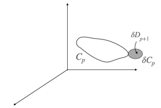
Figure 1: A $(p+1)$-dimensional subspace $\delta D_{p+1}$ with a boundary $\delta C_{p}$.

In particular, when $\delta C_{p}$ has a small support around some point $\xi$ and is given by the boundary of a $(p+1)$-dimensional subspace, i.e., ${}^{\exists}\delta D_{p+1},~{}\partial\delta D_{p+1}=\delta C_{p}$ (see Fig. 1 as an example), Eq. (12) can be also written as

$$\delta\psi[C_{p}]=\frac{1}{(p+1)!}\sigma^{\mu_{1}\cdots\mu_{p+1}}(\delta C_{p})\frac{\delta\psi[C_{p}]}{\delta\sigma^{\mu_{1}\cdots\mu_{p+1}}(\xi)}~{},$$ (13)

where

$$\sigma^{\mu_{1}\cdots\mu_{p+1}}(\delta C_{p}) =\int_{\delta D_{p+1}}dX^{\mu_{1}}\wedge\cdots\wedge dX^{\mu_{p+1}}~{}$$

$$=\int_{\delta D_{p+1}}d(\delta X^{[\mu_{1}}\wedge\cdots\wedge dX^{\mu_{p+1}]})~{}$$

$$=\int_{\delta C_{p}}\delta X^{[\mu_{1}}dX^{\mu_{2}}\wedge\cdots\wedge dX^{\mu_{p+1}]}~{}.$$ (14)

Here, we have used the Stokes theorem in the third line of Eq. (14), and introduced the antisymmetrization,

$$A^{[\mu_{1}\mu_{2}\cdots\mu_{p}]}:=\frac{1}{p!}\sum_{\sigma\in S_{p}}\mathrm{sgn}(\sigma)A^{\sigma(\mu_{1})\sigma(\mu_{2})\cdots\sigma(\mu_{p})}~{},$$ (15)

where $S_{p}$ is the symmetric group of degree $p$, and $\mathrm{sgn}(\sigma)$ is the sign of permutations. We call $\delta\psi[C_{p}]/\delta\sigma^{\mu_{1}\cdots\mu_{p+1}}(\xi)$ the $p$-th order area derivative, which is the generalization of the area derivative for one-dimensional objects [70, 71, 69, 68] to higher-dimensional ones. The definition of the are derivative (13) is abstract, and we should clarify its relation to the ordinary functional derivative (12). Equation (14) can be more explicitly written as

$$\sigma^{\mu_{1}\cdots\mu_{p+1}}(\delta C_{p}) =\int_{\delta C_{p}}d^{p}\xi\sqrt{h}\delta X^{[\mu_{1}}(\xi)E^{\mu_{2}\cdots\mu_{p+1}]}(\xi)~{},$$ (16)

which leads to the following expression of $\delta\psi[C_{p}]$:

$$\delta\psi[C_{p}]=\frac{1}{(p+1)!}\int_{\delta C_{p}}d^{p}\xi\sqrt{h}\delta X^{[\mu_{1}}(\xi)E^{\mu_{2}\cdots\mu_{p+1}]}(\xi)\frac{\delta\psi[C_{p}]}{\delta\sigma^{\mu_{1}\cdots\mu_{p+1}}(\xi)}~{}.$$ (17)

This coincides with Eq. (12) by the identification

$$\frac{\delta\psi[C_{p}]}{\delta X^{\mu_{1}}(\xi)}=\frac{1}{(p+1)!}E^{\mu_{2}\cdots\mu_{p}+1}(\xi)\frac{\delta\psi[C_{p}]}{\delta\sigma^{\mu_{1}\cdots\mu_{p+1}}(\xi)}~{}.$$ (18)

Note that for more general variation $\delta C_{p}$, the above relation does not necessarily hold, and additional terms can appear on the right-hand side.

In particular, the area derivative of the volume integral of a differential $p$ form $A_{p}^{(a)}$ can be calculated in the following way. Under the infinitesimal change $C_{p}+\delta C_{p}$, the variation of Eq. (5) is

$$\int_{\delta C_{p}}A_{p}^{(a)}=\int_{\delta D_{p+1}}dA_{p}^{(a)} =\frac{1}{(p+1)!}\int_{\delta D_{p+1}}dX^{\mu_{p}}\wedge\cdots\wedge dX^{\mu_{p+1}}F_{\mu_{1}\cdots\mu_{p+1}}^{(a)}(X)$$

$$=\frac{1}{(p+1)!}\sigma^{\mu_{1}\cdots\mu_{p+1}}(\delta C_{p})F_{\mu_{1}\cdots\mu_{p+1}}^{(a)}(X)~{},$$ (19)

where

$$F_{p+1}^{(a)}=dA_{p}^{(a)}=\frac{1}{(p+1)!}F_{\mu_{1}\cdots\mu_{p+1}}^{(a)}(X)dX^{\mu_{1}}\wedge\cdots\wedge dX^{\mu_{p+1}}~{}.$$ (20)

The above equation implies

$$\frac{\delta}{\delta\sigma^{\mu_{1}\cdots\mu_{p+1}}(\xi)}\left(\int_{C_{p}}A_{p}^{(a)}\right)=F_{\mu_{1}\cdots\mu_{p+1}}^{(a)}(X)~{}.$$ (21)

Thus, as long as we consider the brane field whose functional form is given by Eq. (3), the area derivative is given by

$$\frac{\delta\psi[C_{p}]}{\delta\sigma^{\mu_{1}\cdots\mu_{p+1}}(\xi)}=\sum_{a}F^{(a)}_{\mu_{1}\cdots\mu_{p+1}}(X(\xi))\frac{\partial\psi(\{z^{a}\})}{\partial z^{a}}\bigg{|}_{z^{a}=\int_{C_{p}}A_{p}^{(a)}}~{}.$$ (22)

It is also convenient to introduce the $(p+1)$-form of the area derivative:

$$D\psi[C_{p}]\coloneqq\frac{1}{(p+1)!}\frac{\delta\psi[C_{p}]}{\delta\sigma^{\mu_{1}\cdots\mu_{p+1}}(\xi)}dX^{\mu_{1}}\wedge\cdots\wedge dX^{\mu_{p+1}}~{}.$$ (23)

Let us see a few important examples below.

Wilson surface
A first important but trivial example is the Wilson surface defined by

$$\psi[C_{p}]=W[C_{p}]\coloneqq\exp\left(i\int_{C_{p}}A_{p}\right)~{},$$ (24)

where $A_{p}$ is a $p$-form field. As already seen before, the area derivative is given by

$$DW[C_{p}]=iW[C_{p}]F_{p+1}~{},$$ (25)

where $F_{p+1}=dA_{p}$ is the field strength.

World volume
The next important example is the world volume,

$$\psi[C_{p}]=\mathrm{Vol}[C_{p}]=\int d^{p}\xi\sqrt{h}~{}.$$ (26)

This case corresponds to $A^{(a)}(X(\xi))=1$ in Eq. (3). Thus, by using Eq. (7), we have

$$D\mathrm{Vol}[C_{p}]=dE_{p}~{}.$$ (27)

Minimal volume
Another example is the (minimal) volume $\mathrm{Vol}[M_{p+1}]$ of a $(p+1)$-dimensional subspace $M_{p+1}$ enclosed by $C_{p}$, i.e., $\partial M_{p+1}=C_{p}$.

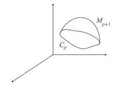
Figure 2: A $(p+1)$-dimensional subspace $M_{p+1}$ with a boundary $C_{p}$.

See Fig. 2 as an example. In this case, we only regard the boundary subspace $C_{p}$ as a physical variable. Since $\mathrm{Vol}[M_{p+1}]$ is given by the $(p+1)$-form integral on $M_{p+1}$, this case does not belong to Eq. (22), but we can calculate its area derivative as follows. A general variation $\delta C_{p}$ can be constructed by adding infinitesimal small loop $\delta C_{p}^{\rm Loop}$ at each point on $C_{p}$. By representing the bulk of $\delta\Gamma_{p}$ as $\delta D_{p+1}$, we have

$$\delta\mathrm{Vol}[M_{p+1}]=\int_{\delta D_{p+1}}E_{p+1}~{},$$ (28)

which corresponds to the expression (2.2). Thus, one can see that $E_{p+1}$ corresponds to $F_{p+1}$ in this case, and we have

$$D\mathrm{Vol}[M_{p+1}]=E_{p+1}~{}.$$ (29)

2.3 Brane field action

Now, we define the brane field action with global $\mathrm{U}(1)$ $p$-form symmetry. At the leading order of the functional-derivative expansion, the action takes the following form,

$$S[\psi] ={\cal N}\int[dC_{p}]\left(-\frac{1}{\mathrm{Vol}[C_{p}]}\int d^{p}\xi\sqrt{h}\frac{\delta\psi^{\dagger}[C_{p}]}{\delta X^{\mu}(\xi)}\frac{\delta\psi[C_{p}]}{\delta X_{\mu}(\xi)}-V(\psi^{\dagger}[C_{p}]\psi[C_{p}])\right)~{},$$ (30)

where Vol$[C_{p}]$ is the world volume (26) and ${\cal N}$ is a normalization factor determined later. As we mentioned in the previous section, the functional derivative contains various area derivatives of lower degrees in general. In this paper, we focus on the $p$-th order area derivative and consider the simplified version of Eq. (30):

$$S_{0}[\psi] ={\cal N}\int[dC_{p}]\left(-\frac{1}{\mathrm{Vol}[C_{p}]}\int_{\Sigma_{d}}\delta(C_{p})D\psi^{\dagger}[C_{p}]\wedge\star D\psi[C_{p}]-V(\psi^{\dagger}[C_{p}]\psi[C_{p}])\right)$$

$$={\cal N}\int[dC_{p}]\Biggl{(}-\frac{1}{(p+1)!\mathrm{Vol}[C_{p}]}\int_{C_{p}}d^{p}\xi\sqrt{h}\frac{\delta\psi^{\dagger}[C_{p}]}{\delta\sigma^{\mu_{1}\cdots\mu_{p+1}}(\xi)}\frac{\delta\psi[C_{p}]}{\delta\sigma_{\mu_{1}\cdots\mu_{p+1}}(\xi)}$$

$$\qquad-V(\psi^{\dagger}[C_{p}]\psi[C_{p}])\Biggr{)}~{},$$ (31)

where $\delta(C_{p})$ is defined as

$$\delta(C_{p})\coloneqq\int_{C_{p}}d^{p}\xi\sqrt{-\frac{h}{g}}\prod_{\mu=0}^{d-1}\delta\left(X^{\mu}-X^{\mu}(\xi)\right)~{}.$$ (32)

Besides, the (path-)integral measure is defined by

$$[dC_{p}]={\cal D}Xe^{-T_{p}\mathrm{Vol}[C_{p}]}~{},$$ (33)

where $T_{p}$ is the $p$-brane tension, and ${\cal D}X$ is the induced measure by the diffeomorphism invariant norm [79],

$$||\delta X||^{2}\coloneqq\int d^{p}\xi\sqrt{h}g_{\mu\nu}(X(\xi))\delta X^{\mu}(\xi)\delta X^{\nu}(\xi)~{}.$$ (34)

The weight in the (path-)integral measure (33) that we choose is nothing but the $p$-brane action [80], which suppresses large branes. Besides, when $\{X^{\mu}(\xi)\}$ represents an embedding of a closed subspace $C_{p}$, its translation $\{X^{\mu}(\xi)+X_{0}^{\mu}\}$ also represents another closed subspace, which means that there are always zero mode integrations in Eq. (33). Equation (2.3) is a straightforward generalization of the action for mean string-field theory [68] to $p$-dimensional brane.

The brane action (2.3) is invariant under the global $\mathrm{U}(1)$ $p$-form transformation,

$$\psi[C_{p}]~{}\rightarrow~{}\exp\left(i\int_{C_{p}}\Lambda_{p}\right)\psi[C_{p}]~{},\quad d\Lambda_{p}=0~{}.$$ (35)

Note that if $C_{p}$ is a boundary, i.e., $C_{p}=\partial C_{p+1}$, the contribution of $\Lambda_{p}$ to the phase vanishes from the Stokes theorem. Even when the topology of space-time is trivial, this transformation is useful as a symmetry, e.g., it leads to Ward-Takahashi identities as in ordinary $p=0$ symmetry.

We can also promote the global symmetry to the gauge symmetry by introducing a $(p+1)$-form gauge field,

$$B_{p+1}=\frac{1}{(p+1)!}B_{p+1,\mu_{1}\cdots\mu_{p+1}}(X)dX^{\mu_{1}}\wedge\cdots\wedge dX^{\mu_{p+1}}~{}$$ (36)

and replacing the derivative with the covariant derivative,

$$\frac{D_{G}\psi[C_{p}]}{\delta\sigma^{\mu_{1}\cdots\mu_{p+1}}(\xi)}\coloneqq\left(\frac{\delta}{\delta\sigma^{\mu_{1}\cdots\mu_{p+1}}(\xi)}-iB_{p+1,\mu_{1}\cdots\mu_{p+1}}(X(\xi))\right)\psi[C_{p}]~{}.$$ (37)

The gauge transformation is given by

$$\psi[C_{p}]~{}\rightarrow~{}e^{i\int_{C_{p}}\Lambda_{p}}\psi[C_{p}]~{},\quad B_{p+1}~{}\rightarrow~{}B_{p+1}+d\Lambda_{p}~{},$$ (38)

where we have used Eq. (25). Note that the action (2.3) is invariant under the spacetime diffeomorphism and the reparametrization on $C_{p}$ by the construction of $\psi[C_{p}]$.

We should comment on the interactions of the brane field. The potential $V(\psi^{\dagger}[C_{p}]\psi[C_{p}])$ in Eq. (2.3) corresponds to contact interactions in ordinary field theory, but we can also consider more general interactions such as [68]

$$\int[dC_{p}^{1}]\int[dC_{p}^{2}]\int[dC_{p}^{3}]\delta(C_{p}^{1}-C_{p}^{2}-C_{p}^{3})\psi^{\dagger}[C_{p}^{1}]\psi[C_{p}^{2}]\psi[C_{p}^{3}]+{\rm h.c.}~{},$$ (39)

which represents the splitting or merging of branes. Such interactions seem to alter the mean-field dynamics of the brane field significantly as the behaviors of phase transition in the ordinary Landau theory change by adding odd potential terms. In this paper, we simply neglect these interactions and focus on the model (2.3).

2.4 Conservation law

As with ordinary symmetry, when $p$-form global symmetry is continuous, we have a current $(p+1)$-form $J_{p+1}$, which is conserved as

$$d\star J_{p+1}=0~{}.$$ (40)

The corresponding conserved charge is given as

$$Q_{p}[\Sigma_{d-p-1}]=\int_{\Sigma_{d-p-1}}\star J_{p+1}~{},$$ (41)

where $\Sigma_{d-p-1}$ is a $(d-p-1)$-dimensional (closed) subspace.

We can calculate $J_{p+1}$ in the brane field theory as follows. Instead of the global $p$-form transformation, we consider an infinitesimal local $p$-form transformation

$$\psi[C_{p}]\quad\rightarrow\quad e^{i\int_{C_{p}}\Lambda_{p}}\psi[C_{p}]~{},\quad d\Lambda_{p}\neq 0~{}.$$ (42)

Then, the variation of the action in the linear order of $\Lambda_{p}$ should have the form

$$\delta S=-\int_{\Sigma_{d}}d\Lambda_{p}\wedge\star J_{p+1}~{},$$ (43)

since the action needs to vanish if $d\Lambda_{p}=0$. $J_{p+1}$ is nothing but the Noether current. From the integrating by part, we obtain

$$\delta S=(-)^{p}\int_{\Sigma_{d}}\Lambda_{p}\wedge d\star J_{p+1}~{}.$$ (44)

If $\psi$ satisfies the equation of motion, the action is stationary, so the divergence of the current vanishes $d\star J_{p+1}=0$.

Let us derive the explicit form of $J_{p+1}$ for the action (2.3). The variation of the action is calculated as

$$\delta S_{0}[\psi] ={\cal N}\int[dC_{p}]\frac{i}{\mathrm{Vol}[C_{p}]}\int_{\Sigma_{d}}\delta(C_{p})\left(d\Lambda_{p}\wedge\star\psi^{\dagger}D\psi-\psi D\psi^{\dagger}\wedge\star d\Lambda_{p}\right)$$

$$={\cal N}\int[dC_{p}]\frac{i}{\mathrm{Vol}[C_{p}]}\int_{\Sigma_{d}}\delta(C_{p})d\Lambda_{p}\wedge\star(\psi^{\dagger}D\psi-\psi D\psi^{\dagger})~{},$$ (45)

where we have used $\eta\wedge\star\omega=\omega\wedge\star\eta$. Comparing Eqs. (43) and (45), we obtain

$$J_{p+1}(X)=-{\cal N}\int[dC_{p}]\frac{\delta(C_{p})}{\mathrm{Vol}[C_{p}]}i(\psi^{\dagger}D\psi-\psi D\psi^{\dagger})~{}.$$ (46)

This expression shows that the $(p+1)$-form current is given by the integral over all the brane configurations. Note that $X$ dependence of the current $J_{p+1}(X)$ comes from $\delta(C_{p})$ in Eq. (32). We can also check that $Q_{p}$ generates the $p$-form transformation (35) in the following way. We formally define the quantum theory of the present brane field by the following path integral:

$$\langle{\cal O}(X(\xi))\rangle\coloneqq\frac{1}{Z}\int{\cal D}\psi{\cal D}\psi^{\dagger}{\cal O}(X(\xi))e^{iS[\psi]}~{}.$$ (47)

Consider the expectation value of $\psi[C_{p}]$,

$$\langle\psi[C_{p}]\dots\rangle~{},$$ (48)

where “$\dots$” represents other arbitrary operators. We choose $\Lambda_{p}$ in the field transformation of Eq. (42) as

$$\Lambda_{p}=\epsilon(-1)^{p(d-p-1)}\delta_{p}(D_{d-p})$$ (49)

with $\partial D_{d-p}=\Sigma_{d-p-1}$, and an infinitesimal parameter $\epsilon$. Here, $\delta_{p}(D_{d-p})$ is the Poincaré-dual form of $D_{d-p}$ such that

$$\int_{D_{d-p}}f_{d-p}=\int_{\Sigma_{d}}f_{d-p}\wedge\delta_{p}(D_{d-p})~{},$$ (50)

for an arbitrary $(d-p)$-form, $f_{d-p}$. $\delta_{p}(D_{d-p})$ can be thought of as a generalization of the delta function.

In this parametrization, the variance of the action (43) is

$$\delta S=\epsilon\int_{\Sigma_{d-p-1}}\star J=\epsilon Q_{p}[\Sigma_{d-p-1}]~{},$$ (51)

while $\psi[C_{p}]$ transforms as

$$\psi[C_{p}]\rightarrow e^{i\int_{C_{p}}\Lambda_{p}}\psi[C_{p}]=e^{i\epsilon(-1)^{p}\mathrm{Link}[\Sigma_{d-p-1},C_{p}]}\psi[C_{p}]~{}.$$ (52)

Here, we have defined the linking number as

$$\mathrm{Link}[\Sigma_{d-p-1},C_{p}]\coloneqq\int_{\Sigma_{d}}\delta_{d-p}(C_{p})\wedge\delta_{p}(D_{d-p})~{}.$$ (53)

See the left figure in Fig. 3 for an example of the configuration of links, where we take $d=3$ and $p=1$. We assume other operators in “$\dots$” do not have support on $D_{d-p}$, so that “$\dots$” does not transform under the field transformation with Eq. (49). In the path-integral, the field transformation (42) is merely a redefinition of the integral variables. Therefore, assuming the path-integral measure is invariant under the field transformation (42), it leads to the identity,

$$\langle\psi[C_{p}]\dots\rangle=\langle e^{i\epsilon Q_{p}[\Sigma_{d-p-1}]+i\epsilon(-1)^{p}\mathrm{Link}[\Sigma_{d-p-1},C_{p}]}\psi[C_{p}]\dots\rangle~{}.$$ (54)

This implies

$$Q_{p}[\Sigma_{d-p-1}]\psi[C_{p}]=-(-1)^{p}\mathrm{Link}[\Sigma_{d-p-1},C_{p}]\psi[C_{p}]~{}.$$ (55)

This is the relation in the path integral. To derive the relation in the operator formalism, consider the Cauchy surface labeled by time $t$. Let $C_{d-p-1}(t_{0})$ be $(d-p-1)$-dimensional subspace on the Cauchy surface at $t=t_{0}$. We choose that $\Sigma_{d-p-1}=C_{d-p-1}(t_{0}+\eta)\cup\overline{C_{d-p-1}}(t_{0}-\eta)$ with an infinitesimal parameter $\eta$. Here, $\overline{C_{d-p-1}}$ is the $(d-p-1)$-dimensional subspace with the opposite orientation of $C_{d-p-1}$. We also choose that $C_{p}$ is a $p$-dimensional subspace on the Cauchy surface at $t=t_{0}$. See the right figure in Fig. 3 for the configuration. In this configuration, the left-hand side in Eq. (55) becomes

$$Q_{p}[\Sigma_{d-p-1}]\psi[C_{p}]=Q_{p}[C_{d-p-1}(t_{0}+\eta)]\psi[C_{p}]-Q_{p}[C_{d-p-1}(t_{0}-\eta)]\psi[C_{p}]~{}.$$ (56)

In operator formalism, the ordering of the operator product corresponds to the time ordering, so $Q_{p}[C_{d-p-1}(t_{0}+\eta)]\psi[C_{p}]-Q_{p}[C_{d-p-1}(t_{0}-\eta)]\psi[C_{p}]\to[Q_{p}[C_{d-p-1}],\psi[C_{p}]]$; thus, we find that the Noether charge $Q_{p}$ generates the symmetry transformation,

$$[iQ_{p}[C_{d-p-1}],\psi[C_{p}]]=-i\mathrm{I}[C_{d-p-1},C_{p}]\psi[C_{p}]~{}.$$ (57)

Here, $\mathrm{I}[C_{d-p-1},C_{p}]$ represents the intersection number between $C_{d-p-1}$ and $C_{p}$ on the Cauchy surface, which can be obtained by evaluating the right-hand side in Eq. (55) with $\Sigma_{d-p-1}=C_{d-p-1}(t_{0}+\eta)\cup\overline{C_{d-p-1}}(t_{0}-\eta)$.

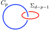
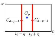
Figure 3: (Left) Configuration of the link between $C_{p}$ and $\Sigma_{d-p-1}$ for $d=3$ and $p=1$. (Right) Configuration of $C_{p}$ and $C_{d-p-1}$ to obtain the commutation relation in operator formalism. The arrows indicate the orientation of the subspace.

3 Spontaneous breaking of Higher-form symmetry

In this section, we discuss the spontaneous breaking of the higher-form symmetry in the brane field theory. As in the case of $0$-form symmetry, gapless modes appear when the continuous $p$-form symmetry is spontaneously broken [3, 75, 76, 81]. For $0$-form symmetry, the symmetry breaking is characterized by an order parameter that is the expectation value of a local field $\langle\phi(x)\rangle$. This order parameter cannot be directly extended to higher-form symmetries. Alternatively, we can use the off-diagonal long-range order,

$$O_{0}=\lim_{|x-y|\to\infty}\langle\phi^{\dagger}(x)\phi(y)\rangle\simeq\langle\phi^{\dagger}(x)\rangle\langle\phi(y)\rangle~{},$$ (58)

as the order parameter. Since the two points $(x,y)$ can be written as the boundary of segment $M_{1}$ and the distance between $x$ and $y$ can be expressed as the minimal volume $|x-y|=\mathrm{Vol}(M_{1})$, the order parameter can be written in the form:

$$O_{0}=\lim_{\mathrm{Vol}[M_{1}]\to\infty}\langle\phi^{\dagger}(x)\phi(y)\rangle~{}.$$ (59)

This expression can be naturally extended to accommodate the case of $p$-form symmetry. In this context, we can define the order parameter as

$$O_{p}=\lim_{\mathrm{Vol}[M_{p+1}]\to\infty}\langle\psi[C_{p}]\rangle~{},$$ (60)

where $\partial M_{p+1}=C_{p}$. We will use Eq. (60) as the order parameter of spontaneous breaking of $p$-form symmetry. In general, the order parameter defined in Eq. (60) might vanish in the limit of large $M_{p+1}$, depending on $C_{p}=\partial M_{p+1}$, i.e., the perimeter law. In such cases, it is necessary to consider a renormalized order operator $\langle Z(C_{p})\psi[C_{p}]\rangle$ with a field-independent functional $Z(C_{p})$. If the order operator does not vanish no matter what renormalization is performed, we can say that the symmetry is spontaneously broken.

We work within the mean-field approximation. As an ansatz for the solution, we assume that the brane-field configuration $\psi[C_{p}]$ depends only on the minimum volume with the boundary $C_{p}$,

$$\psi[C_{p}]=\frac{1}{\sqrt{2}}f(z=\mathrm{Vol}[M_{p+1}])~{},\quad\partial M_{p+1}=C_{p}~{}.$$ (61)

This corresponds to the truncated treatment in Ref. [68]. See also Appendix B for more general truncations. By using Eq. (29), the area derivative becomes

$$D\psi[C_{p}]=\frac{1}{\sqrt{2}}E_{p+1}f^{\prime}(z)~{},$$ (62)

which leads to

$$D\psi^{\dagger}\wedge\star D\psi=\frac{1}{2}f^{\prime}(z)^{2}E_{p}\wedge\star E_{p}=\sqrt{-g}\frac{1}{2}f^{\prime}(z)^{2}dX^{0}\wedge\cdots\wedge dX^{d-1}~{}.$$ (63)

Here, we used Eq. (10) to evaluate $E_{p}\wedge\star E_{p}$. Then, the action (2.3) becomes

$$S_{0}[f] =-{\cal N}\int[dC_{p}]\left(\frac{f^{\prime}(z)^{2}}{2\mathrm{Vol}[C_{p}]}\int_{C_{p}}d^{p}\xi\sqrt{h}+V(f(z)^{2})\right)\bigg{|}_{z=\mathrm{Vol}[M_{p+1}]}$$

$$=-{\cal N}\int{\cal D}Xe^{-T_{p}\mathrm{Vol}[C_{p}]}\left(\frac{1}{2}f^{\prime}(z)^{2}+V(f(z)^{2})\right)\bigg{|}_{z=\mathrm{Vol}[M_{p+1}]}$$

$$=-\int_{0}^{\infty}dzg(z)\left(\frac{1}{2}f^{\prime}(z)^{2}+V(f(z)^{2})\right)~{},$$ (64)

where

$$g(z)={\cal N}\int{\cal D}Xe^{-T_{p}\mathrm{Vol}[C_{p}]}\delta(z-\mathrm{Vol}[M_{p+1}])$$ (65)

is the density of $p$-brane configurations for a given minimal volume $z$. The equation of motion for $f(z)$ is

$$\frac{d}{dz}\left(g(z)f^{\prime}(z)\right)-g(z)\frac{\partial V}{\partial f}=0~{},$$ (66)

$$\therefore\quad f^{\prime\prime}(z)+\frac{g^{\prime}(z)}{g(z)}f^{\prime}(z)-\frac{\partial V}{\partial f}=0~{}.$$ (67)

By introducing the WKB form $f(z)=\exp(S(z))$, Eq. (67) can be also rewritten as

$$S^{\prime\prime}(z)+S^{\prime}(z)^{2}+\frac{g^{\prime}(z)}{g(z)}S^{\prime}(z)-\frac{1}{f(z)}\frac{\partial V}{\partial f}=0~{}.$$ (68)

As in the usual Landau theory, the vacuum state is determined by the potential $V(f^{2})$. As a simplest example, let us consider the following potential:

$$V(f^{2}) =m(\psi^{\dagger}\psi)+\frac{\lambda}{4}(\psi^{\dagger}\psi)^{2}$$

$$=\frac{m}{2}f^{2}+\frac{\lambda}{8}f^{4}~{}.$$ (69)

In the following, we always assume $\lambda>0$ to guarantee the stability of the system.

3.1 Unbroken phase

When $m>0$, the minimum of the potential is located at $f=0$. Therefore, we can neglect the quartic potential in the equation of motion as

$$S^{\prime\prime}(z)+S^{\prime}(z)^{2}+\frac{g^{\prime}(z)}{g(z)}S^{\prime}(z)-m\approx 0~{}.$$ (70)

Let us find the asymptotic solution for the large volume. For $z\rightarrow\infty$, we have $g^{\prime}(z)/g(z)\sim z^{-1}$ from dimensional analysis and the solution is given by

$$S[z]\approx-\sqrt{m}z~{},$$ (71)

which corresponds to the area law of the brane field

$$\psi[C_{p}]=c\exp\left(-\sqrt{m}\mathrm{Vol}[M_{p+1}]\right)\quad\text{for Vol$[M_{p+1}]\rightarrow\infty$}~{},$$ (72)

where $c$ is a constant that in principle can be determined if we specify the boundary condition for $z\rightarrow 0$ (small brane limit). The exponential behavior also justifies neglecting the quartic potential term in the equation of motion. This implies that the order parameter vanishes, indicating the unbroken phase of $p$-form symmetry.

Equation (72) should be compared to the correlation function of the ordinary field theory ($p=0$):

$$\langle\phi^{\dagger}(x)\phi(y)\rangle\sim e^{-\frac{|x-y|}{\xi(m)}}~{},\quad\xi(m)\propto\frac{1}{m^{1/2}}~{}.$$ (73)

In the $p$-form case, Eq. (72) means

$$(\text{volume tension})\sim m^{1/2}$$ (74)

within the mean-field approximation.

3.2 Broken phase

Let us next consider the case for $m<0$. Within the truncated approximation, the equation of motion is given by Eq. (67):

$$f^{\prime\prime}(z)+\frac{g^{\prime}(z)}{g(z)}f^{\prime}(z)-mf(z)-\frac{\lambda}{2}f(z)^{3}=0~{}.$$ (75)

As in the unbroken case, we focus on the large $z$ behavior. In this case, we can neglect the derivative terms for $z\rightarrow\infty$ by dimensional analysis, and the solution is given by $f(z)^{2}=v^{2}\coloneqq-2m/\lambda$. Since the order parameter $\psi[C_{p}]=v/\sqrt{2}$ is nonvanishing at $z\to\infty$, the $p$-form symmetry is spontaneously broken.

In ordinary quantum field theory, the non-renormalized order parameter exhibits a perimeter law in the broken phase. However, the order parameter is completely independent of $C_{p}$ in the present model. As already mentioned in Ref. [68], this may be an artifact by having neglected the topology-changing terms such as Eq. (39). It would be interesting to see whether we can actually realize the perimeter law by adding such topology-changing interactions.

3.3 Nambu-Goldstone modes

What are the low-energy fluctuation modes in the broken phase? As in the case of $0$-form symmetry, the phase fields are candidates for low-energy degrees of freedom (d.o.f):

$$\psi[C_{p}]=\frac{v}{\sqrt{2}}\exp\left(i\int_{C_{p}}A_{p}\right)~{},\quad A_{p}=\frac{1}{p!}A_{p,\mu_{1}\cdots\mu_{p}}(X)dX^{\mu_{1}}\wedge\cdots\wedge dX^{\mu_{p}}~{}.$$ (76)

Let us see how this d.o.f describes a gapless mode in the effective action. Note that the effective theory has the gauge symmetry

$$A_{p}\quad\rightarrow\quad A_{p}+d\Lambda_{p-1}~{},\quad d\Lambda_{p-1}\neq 0~{},$$ (77)

because Eq. (76) is invariant under this transformation due to the closedness of $C_{p}$. Here $\Lambda_{p-1}$ is $(p-1)$-form gauge parameter. For Eq. (76) to be invariant, the integral of $d\Lambda_{p-1}$ need not vanish, but can be

$$\int_{C_{p}}d\Lambda_{p-1}\in 2\pi\mathbb{Z}~{}.$$ (78)

In other words, $A_{p}$ is the $\mathrm{U}(1)$ $p$-form gauge field.

Now let us calculate the effective action for $A_{p}$. By putting Eq. (76) into the action (2.3) and using Eq. (25), we have

$$S_{0}[A_{p}]=-{\cal N}\int[dC_{p}]\left(\frac{v^{2}}{2(p+1)!\mathrm{Vol}[C_{p}]}\int_{C_{p}}d^{p}\xi\sqrt{h}F^{\mu_{1}\cdots\mu_{p+1}}(X(\xi))F_{\mu_{1}\cdots\mu_{p+1}}(X(\xi))\right)~{}.$$ (79)

In the following, we consider the flat spacetime $g_{\mu\nu}=\eta_{\mu\nu}$ for simplicity. By introducing the Fourier modes,

$$F(x)\coloneqq v^{2}F^{\mu_{1}\cdots\mu_{p+1}}(x)F_{\mu_{1}\cdots\mu_{p+1}}(x)=\int\frac{d^{d}k}{(2\pi)^{d}}e^{ik\cdot x}\tilde{F}(k)~{},$$ (80)

Eq. (79) can be written as

$$S_{0}[A_{p}]=-\int\frac{d^{d}k}{(2\pi)^{d}}K(k)\tilde{F}(k)~{},$$ (81)

where

$$K(k)={\cal N}\int{\cal D}X\frac{1}{2(p+1)!\mathrm{Vol}[C_{p}]}\int_{C_{p}}d^{p}\xi\sqrt{h}e^{-T_{p}\mathrm{Vol}[C_{p}]+ik_{\mu}X^{\mu}(\xi)}~{}.$$ (82)

There are zero-mode integrations in the above path-integral, and it is convenient to separate them:

$$K(k)={\cal N}\int d^{d}xe^{ik\cdot x}\int{\cal D}X_{\mathrm{NZ}}\frac{1}{2(p+1)!\mathrm{Vol}[C_{p}]}\int_{C_{p}}d^{p}\xi\sqrt{h}e^{-T_{p}\mathrm{Vol}[C_{p}]+ik_{\mu}X_{\mathrm{NZ}}^{\mu}(\xi)}~{},$$ (83)

where $X_{\mathrm{NZ}}^{\mu}(\xi)$ denotes the nonzero mode. In this expression, it is easy to see that $K(k)$ is proportional to $\delta^{(d)}(k)$. Thus, we can choose the normalization ${\cal N}$ as

$${\cal N}\int{\cal D}X_{\mathrm{NZ}}\frac{1}{\mathrm{Vol}[C_{p}]}\int_{C_{p}}d^{p}\xi\sqrt{h}e^{-T_{p}\mathrm{Vol}[C_{p}]}=1~{}\leftrightarrow~{}K(k)=\frac{(2\pi)^{d}}{2(p+1)!}\delta^{(d)}(k)~{},$$ (84)

which leads to

$$S_{0}[A_{p}] =-\frac{1}{2(p+1)!}\tilde{F}(0)$$

$$=-\frac{v^{2}}{2(p+1)!}\int d^{d}xF^{\mu_{1}\cdots\mu_{p+1}}(x)F_{\mu_{1}\cdots\mu_{p+1}}(x)$$

$$=-\frac{v^{2}}{2}\int_{\Sigma_{d}}F_{p+1}\wedge\star F_{p+1}~{},$$ (85)

which is nothing but the $p$-form Maxwell theory, and thus, $A_{p}$ is gapless for $d>p+2$ .

3.4 Other fluctuation modes

What about the other fluctuation modes? In general, they are given by expanding the phase with respect to the derivatives of $X^{\mu}(\xi)$:

$$\psi[C_{p}] =\frac{v}{\sqrt{2}}\exp\left(i\int_{C_{p}}d^{p}\xi\sqrt{h}\left\{\phi(X(\xi))+h^{ij}(\xi)\frac{\partial X^{\mu}}{\partial\xi^{i}}\frac{\partial X^{\nu}}{\partial\xi^{j}}H_{\mu\nu}(X(\xi))+\cdots\right\}\right)~{},$$ (86)

where $\phi(X)$ is a scalar field and $H_{\mu\nu}(X)$ is a symmetric tensor field. These fluctuation modes are typically gapped because they are not protected by spontaneous symmetry breaking.

Here, we actually show that $\phi(X)$ is gapped as an example. The area derivative is calculated as

$$D\int_{C_{p}}d^{p}\xi\sqrt{h}\phi(X(\xi))=d(\phi E_{p})=\frac{(p+1)}{(p+1)!}\partial_{[\mu_{1}}\left(\phi E_{\mu_{2}\cdots\mu_{p+1}]}\right)dX^{\mu_{1}}\wedge\cdots\wedge dX^{\mu_{p+1}}~{}.$$ (87)

Then, we have

$$D\psi^{\dagger}\wedge\star D\psi=\frac{v^{2}\sqrt{-g}(p+1)^{2}}{2(p+1)!}\partial_{[\mu_{1}}\left(\phi E_{\mu_{2}\cdots\mu_{p+1}]}\right)\partial^{[\mu_{1}}\left(\phi E^{\mu_{2}\cdots\mu_{p+1}]}\right)dX^{0}\wedge\cdots dX^{d-1}~{},$$ (88)

Now, the effective action is written as

$$S_{0}[\phi] =-{\cal N}\int[dC_{p}]\frac{v^{2}}{2\mathrm{Vol}[C_{p}]}\int_{C_{p}}d^{p}\xi\sqrt{h}$$

$$\quad\times\left(\frac{(p+1)^{2}}{(p+1)!}(\partial_{[\mu_{1}}\phi)E_{\mu_{2}\cdots\mu_{p+1}]}(\partial^{[\mu_{1}}\phi)E^{\mu_{2}\cdots\mu_{p+1}]}+M^{2}\phi^{2}+2\phi\partial_{\mu}\phi G^{\mu}\right)~{},$$ (89)

where

$$G^{\mu}(X(\xi)) =\frac{(p+1)^{2}}{(p+1)!}E_{\mu_{1}\cdots\mu_{p}}\partial^{[\mu}E^{\mu_{1}\cdots\mu_{p}]}~{},$$ (90)

$$M^{2}(X(\xi)) =\frac{(p+1)^{2}}{(p+1)!}\partial_{[\mu_{1}}E_{\mu_{2}\cdots\mu_{p+1}]}\partial^{[\mu_{1}}E^{\mu_{2}\cdots\mu_{p+1}]}~{}.$$ (91)

The first term in Eq. (89) can be expressed as

$$\frac{(p+1)^{2}}{(p+1)!}(\partial_{[\mu_{1}}\phi)E_{\mu_{2}\cdots\mu_{p+1}]}(\partial^{[\mu_{1}}\phi)E^{\mu_{2}\cdots\mu_{p+1}]}$$

$$=\frac{1}{(p+1)!}\Bigl{(}(\partial_{\mu_{1}}\phi)E_{\mu_{2}\mu_{3}\cdots\mu_{p+1}}-(\partial_{\mu_{2}}\phi)E_{\mu_{1}\mu_{3}\cdots\mu_{p+1}}\cdots-(\partial_{\mu_{p+1}}\phi)E_{\mu_{2}\mu_{3}\cdots\mu_{1}}\Bigr{)}$$

$$\quad\times\Bigl{(}(\partial^{\mu_{1}}\phi)E^{\mu_{2}\mu_{3}\cdots\mu_{p+1}}-(\partial^{\mu_{2}}\phi)E^{\mu_{1}\mu_{3}\cdots\mu_{p+1}}\cdots-(\partial^{\mu_{p+1}}\phi)E^{\mu_{2}\mu_{3}\cdots\mu_{1}}\Bigr{)}$$

$$=\frac{1}{(p+1)!}\Bigl{(}(p+1)(\partial_{\mu}\phi)(\partial^{\mu}\phi)E_{\mu_{1}\mu_{2}\cdots\mu_{p}}E^{\mu_{1}\mu_{2}\cdots\mu_{p}}$$

$$\qquad\qquad\qquad-p(p+1)(\partial_{\mu}\phi)(\partial^{\nu}\phi)E_{\nu\mu_{1}\mu_{2}\cdots\mu_{p-1}}E^{\mu\mu_{1}\mu_{2}\cdots\mu_{p-1}}\Bigr{)}$$

$$=(g^{\mu\nu}-e_{i}^{\mu}e_{j}^{\nu}h^{ij})(\partial_{\mu}\phi)(\partial_{\nu}\phi)$$

$$=n^{\mu}n^{\nu}(\partial_{\mu}\phi)(\partial_{\nu}\phi)~{},$$ (92)

where $n^{\mu}$ is the normal vector on $C_{p}$, and we have used $g^{\mu\nu}=n^{\mu}n^{\nu}+h^{ij}e_{i}^{\mu}e_{j}^{\nu}$ in the last line. Now let us focus on the flat spacetime $g_{\mu\nu}=\eta_{\mu\nu}$ for simplicity. Equation (92) gives the kinetic term

$$-\frac{1}{2}\int d^{d}x\langle n^{\mu}n^{\nu}\rangle\partial_{\mu}\phi\partial_{\mu}\phi~{},$$ (93)

where

$$\langle n^{\mu}n^{\nu}\rangle={\cal N}\int{\cal D}X_{\rm NZ}\frac{v^{2}}{\mathrm{Vol}[C_{p}]}\int_{C_{p}}d^{p}\xi\sqrt{h}e^{-T_{p}\mathrm{Vol}[C_{p}]}n^{\mu}(\xi)n^{\nu}(\xi)~{},$$ (94)

which has to be proportional to $\eta^{\mu\nu}$ as long as the Lorentz symmetry is unbroken. As a result, Eq. (93) gives the usual kinetic.

For the evaluation of the other terms in Eq. (89), note that $E_{p}$ (and correspondingly $G^{\mu}$ and $M^{2}$) does not depend on the spacetime zero mode $x^{\mu}$ by definition. Then, the second term becomes the mass term

$$-\frac{v^{2}\Lambda^{2}}{2}\int d^{d}x\phi(x)^{2}~{},$$ (95)

where $\Lambda^{2}$ is defined by

$$\Lambda^{2}={\cal N}\int{\cal D}X_{\mathrm{NZ}}\frac{1}{\mathrm{Vol}[C_{p}]}\int_{C_{p}}d^{p}\xi\sqrt{h}e^{-T_{p}\mathrm{Vol}[C_{p}]}M^{2}(X_{\mathrm{NZ}}(\xi))~{},$$ (96)

which can be interpreted as a bare mass of $\phi(x)$. As for the third term, it contains the following average:

$$\langle G^{\mu}\rangle={\cal N}\int{\cal D}X_{\mathrm{NZ}}\frac{1}{\mathrm{Vol}[C_{p}]}\int_{C_{p}}d^{p}\xi\sqrt{h}e^{-T_{p}\mathrm{Vol}[C_{p}]}G^{\mu}(X_{\mathrm{NZ}}(\xi))~{}.$$ (97)

This term should vanish as long as the spacetime symmetry is not spontaneously broken. Now, one can see that the scalar mode is gapped. Other fluctuation modes also become gapped as long as they are not protected by some additional symmetry of the original brane-field theory.

3.5 Emergent higher-form symmetry

In the case of ordinary $0$-form symmetries, there exists a vortex solution in the broken phase, which carries the topological charge given by

$$Q_{d-2}=\frac{1}{2\pi v^{2}}\oint_{S_{1}}J_{1}~{},\quad J_{1}=j_{\mu}dx^{\mu}~{},\quad j_{\mu}=-i(\phi^{*}\partial_{\mu}\phi-\phi\partial_{\mu}\phi^{*})~{},$$ (98)

where $\phi$ is a complex scalar field, and $S_{1}$ is a closed curve. This symmetry is not exact but rather emergent, as this charge is not strictly conserved,

$$dJ_{1}=-2id\phi^{*}\wedge d\phi~{}.$$ (99)

If we parametrize $\phi=he^{i\varphi}/\sqrt{2}$, where $h$ and $\varphi$ are the radial and phase degrees of freedom, respectively, the current is expressed as $J_{1}=h^{2}d\varphi$, leading to $dJ_{1}=2hdh\wedge d\varphi$. Away from the vortex core, $h$ approaches the vacuum expectation value (VEV) $h=v$, and the fluctuation of $h$ can be neglected at low energy because it is gapped. Consequently, $J_{1}$ can be approximated as $J_{1}\approx v^{2}d\varphi$, and the topological charge reduces to

$$Q_{d-2}=\oint\frac{d\varphi}{2\pi}~{},$$ (100)

which is conserved due to $dd\varphi=0$. $U(\theta)=e^{i\theta Q_{d-2}}$ is the corresponding symmetry operator, which acts on $(d-2)$-dimensional object, i.e., $\mathrm{U}(1)$ $(d-2)$-form symmetry. For example, for $d=4$, this is $2$-form symmetry, and the $2$-dimensional object is the worldsurface of a vortex.

In the case of $p$-form symmetry, a natural generalization of topological charge is given by

$$Q_{d-p-2}=\frac{1}{2\pi v^{2}}\int_{S_{p+1}}J_{p+1}~{},$$ (101)

where $S_{p+1}$ is a closed $(p+1)$-dimensional subspace and $J_{p+1}$ is given in Eq. (46). By substituting Eq. (76) into Eq. (46), we obtain $J_{p+1}=v^{2}F_{p+1}$, which can also be derived from the low-energy effective action (3.3), using the Noether theorem. Consequently, the topological charge (101) becomes

$$Q_{d-p-2}=\int_{S_{p+1}}\frac{{F}_{p+1}}{2\pi}~{}.$$ (102)

The corresponding symmetry operator is $U(\theta)=e^{i\theta Q_{d-p-2}}$ and the charged object is a $(d-p-2)$-dimensional object. For example, when $d=4$ and $p=1$, the charged object is a worldline of a magnetic particle. Since $A_{p}$ is the $\mathrm{U}(1)$ $p$-form gauge field, it satisfies the Dirac quantization condition,

$$\int_{S_{p+1}}F_{p+1}\in 2\pi\mathbb{Z}~{},$$ (103)

which also leads to

$$Q_{d-p-2}\in\mathbb{Z}~{}.$$ (104)

3.6 Discrete higher-form symmetry breaking

Up to this point, we have discussed the case with a continuous higher-form symmetry. In general, we can consider a model with a discrete higher-form symmetry and its spontaneous breaking. For example, we can construct a model with $\mathbb{Z}_{N}$ $p$-form symmetry, by adding the following term

$$-\lambda_{N}\left\{(\psi[C_{p}])^{N}+(\psi^{\dagger}[C_{p}])^{N}\right\}~{},$$ (105)

which explicitly breaks the $\mathrm{U}(1)$ $p$-form symmetry down to $\mathbb{Z}_{N}$, into Eq. (2.3). Correspondingly, the VEV is discretized as

$$\psi[C_{p}]=\frac{v}{\sqrt{2}}\exp\left(\frac{2\pi ik}{N}\right)~{},\quad k=1,2,\cdots,N~{},$$ (106)

in a broken phase of $\mathbb{Z}_{N}$ $p$-form symmetry. In this case, the phase degrees of freedom,

$$\psi[C_{p}]=\frac{v}{\sqrt{2}}\exp\left(i\int_{C_{p}}A_{p}\right)~{},$$ (107)

will no longer be gapless.

The effective theory must be invariant under $\mathbb{Z}_{N}$ $p$-form symmetry corresponding to the shift,

$$A_{p}~{} \rightarrow~{}A_{p}+\frac{n}{N}\Lambda_{p}~{},\quad d\Lambda_{p}=0~{},$$ (108)

with $\int_{C_{p}}\Lambda_{p}\in 2\pi\mathbb{Z}$, where $n\in\mathbb{Z}$. For example, when $p=0$, $\int_{C_{p=0}}A_{p=0}=\varphi(x)$ is the periodic scalar field, and it has the periodic potential $V(\varphi)=V(\varphi+2\pi/N)$. The effective theory must also be invariant under gauge transformation of $A_{p}$,

$$A_{p}~{}\rightarrow~{}A_{p}+d\Lambda_{p-1}~{},$$ (109)

with $\int_{C_{p}}d\Lambda_{p-1}\in 2\pi\mathbb{Z}$, which is a redundancy in the degrees of freedom of Eq. (107).

When the discrete higher-form symmetry is spontaneously broken, it exhibits topological order. The degeneracy of the ground state depends on the topology of the space. We assume that the space manifold has a nontrivial topology such as $\Sigma_{d-1}=C_{p+1}\times D_{d-p-2}$, where $C_{p+1}$ is a $(p+1)$-dimensional subspace with boundaries at infinity $C_{p}^{{}^{\prime}\infty}$ and $C_{p}^{\infty}$, and $D_{d-p-2}$ is a $(d-p-2)$-dimensional subspace. See Fig. 4 as an example. We also assume that $C_{p}^{{}^{\prime}\infty}$ and $C_{p}^{\infty}$ are not contractible, so that the $p$-form symmetry can act nontrivially. In such a case, there exists a classical static configuration $\psi_{W}[C_{p}]=v\exp\left(i\int_{C_{p}}A_{p}^{W}\right)$ connecting different ground states. Note that in the case of $0$-form symmetry, which exhibits not a topological order but a spontaneous breaking of discrete symmetry, the topological defect connecting the different ground states is nothing but a domain wall. The corresponding topological charge is given by

$$Q_{d-p-2}=\frac{N}{2\pi}\int_{C_{p+1}}dA_{p}=\frac{N}{2\pi}\left(\int_{C_{p}^{{}^{\prime}\infty}}-\int_{C_{p}^{\infty}}\right)A_{p}~{},$$ (110)

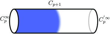
Figure 4: $C_{p+1}$ for $p=1$. Blue and white colors correspond to different vacua.

More explicitly, $dA_{p}^{W}$ can be represented as

$$dA_{p}^{W}=\frac{2\pi}{N}\delta_{p+1}(D_{d-p-1}^{W})~{},$$ (111)

in the thin wall limit, where $\delta_{p+1}(D_{d-p-1}^{W})$ is the Poincaré-dual form defined in Eq. (50). Here, $D_{d-p-1}^{W}$ corresponds to the worldvolume of $D_{d-p-2}$.

Now, let us study the low-energy effective theory. We generalize the argument of $0$-form symmetry discussed in Ref. [77] to the brane field theory. To derive the effective theory, we rewrite Eq. (105) for large $v$ as

$$-\lambda_{N}\left\{(\psi[C_{p}])^{N}+(\psi^{\dagger}[C_{p}])^{N}\right\} =-2^{-\frac{N}{2}}\lambda_{N}{v^{N}}\cos\left(N\int_{C_{p}}A_{p}\right)$$

$$\to 2^{-\frac{N}{2}-1}\lambda_{N}v^{N}\left(N\int_{C_{p}}A_{p}-2\pi n\right)^{2}~{}.$$ (112)

In the last line, we approximated the cosine by using the Villain formula [82],

$$\exp({\beta\cos\theta})\approx\sum_{n\in\mathbb{Z}}\exp\left({\beta-\frac{1}{2}\beta(\theta-2\pi n)^{2}}\right)~{},$$ (113)

for large $\beta$, and dropped the constant term. Equation (3.6) is gauge invariant under Eq. (109) accompanied by the shift of $n$, $n\to n+N\int_{C_{p}}d\Lambda_{p-1}/(2\pi)$. Similarly, it is invariant under $\mathbb{Z}_{N}$ transformation (108). We can replace the integer $n$ in Eq. (3.6) by introducing the flat $\mathrm{U}(1)$ gauge field ${f}_{p}$, as $N\int_{C_{p}}A_{p}-2\pi n=\int_{C_{p}}(NA_{p}-{f}_{p})$, where $\int_{C_{p}}{f}_{p}\in 2\pi\mathbb{Z}$.

By performing the same calculations as in Sec. 3.3, we have the following effective action of $A_{p}$:

$$S[A] =-\frac{v^{2}}{2}\int_{\Sigma_{d}}F_{p+1}\wedge\star F_{p+1}-\frac{\tilde{\lambda}_{N}}{2}\int_{\Sigma_{d}}(NA_{p}-f_{p})\wedge\star(NA_{p}-f_{p})-\frac{1}{2\pi}\int_{\Sigma_{d}}B_{d-p-1}\wedge df_{p}~{},$$ (114)

where $\tilde{\lambda}_{N}$ is a coupling constant which includes $\lambda_{N}$. See Appendix C for the derivation of the mass term. Here, $f_{p}$ is the $\mathrm{U}(1)$ $p$-form gauge field, and the flatness condition is imposed by the last term by using the Lagrange multiplier $B_{d-p-1}$. On the other hand, $f_{p}$ can be eliminated using the equation of motion for $f_{p}$,

$$f_{p}=NA_{p}+\frac{(-1)^{d-p}}{2\pi{\tilde{\lambda}}_{N}}\star dB_{d-p-1}~{},$$ (115)

which leads to

$$-\frac{1}{8\pi^{2}\tilde{\lambda}_{N}}\int_{\Sigma_{d}}dB_{d-p-1}\wedge\star dB_{d-p-1}+\frac{1}{4\pi^{2}\tilde{\lambda}_{N}}\int_{\Sigma_{d}}d(B_{d-p-1}\wedge\star dB_{d-p-1})$$

$$\quad-\frac{v^{2}}{2}\int_{\Sigma_{d}}F_{p+1}\wedge\star F_{p+1}-\frac{N}{2\pi}\int_{\Sigma_{d}}B_{d-p-1}\wedge dA_{p}~{}.$$ (116)

For the domain wall configuration (111), the last term becomes

$$\frac{N}{2\pi}\int_{\Sigma_{d}}B_{d-p-1}\wedge dA_{p}=\int_{D_{d-p-1}^{W}}B_{d-p-1},$$ (117)

which implies that the worldvolume $D_{d-p-1}^{W}$ couples with the gauge field $B_{d-p-1}$.

In the low-energy limit, we can neglect higher derivative terms, and we obtain the topological field theory with the action,

$$S_{\rm top}=-\frac{N}{2\pi}\int_{\Sigma_{d}}B_{d-p-1}\wedge dA_{p}~{}.$$ (118)

This effective theory has the following emergent global $\mathbb{Z}_{N}$ $(d-p-1)$-form symmetry:

$$B_{d-p-1}~{} \rightarrow~{}B_{d-p-1}+\frac{n}{N}\Lambda_{d-p-1}~{},\quad d\Lambda_{d-p-1}=0,\quad n\in\mathbb{Z}~{},$$ (119)

with

$$\int_{C_{d-p-1}}\Lambda_{d-p-1}\in 2\pi\mathbb{Z}~{},$$ (120)

in addition to the original $\mathbb{Z}_{N}$ $p$-form symmetry (108), where $C_{d-p-1}$ is a $(d-p-1)$-dimensional closed subspace. The charged objects for $p$- and $(d-p-1)$-form symmetries are the Wilson surfaces:

$$W[C_{p}]=\exp\left(i\int_{C_{p}}A_{p}\right)~{},\quad V[C_{d-p-1}]=\exp\left(i\int_{C_{d-p-1}}B_{d-p-1}\right)~{},$$ (121)

respectively. We can also show that $V[C_{d-p-1}]$ and $W[C_{p}]$ correspond to the symmetry operators of the above $p$ and $(d-p-1)$-form symmetries. They satisfy

$$\langle V[C_{d-p-1}]W[C_{p}]\dots\rangle=e^{\frac{2\pi i}{N}\mathrm{Link}[C_{p},C_{d-p-1}]}\langle W_{q}[C_{p}]\dots\rangle~{},$$ (122)

where $\mathrm{Link}[C_{p},C_{d-p-1}]$ is the linking number defined in Eq. (53), and “$\dots$” denotes other operators that neither link nor intersect $C_{d-p-1}$.

As mentioned above, this theory (118) exhibits the grand state degeneracy depending on the topology of the spatial manifold $\Sigma_{d-1}$. Let us look at this in detail using the same argument in Sec. 2.4. When $\Sigma_{d-1}=S^{p}\times S^{d-p-1}$, we can choose $C_{p}=S^{p}$ and $C_{d-p-1}=S^{d-p-1}$. Consider $V[C_{d-p-1}]W[C_{p}]V^{-1}[C_{d-p-1}]$ in the operator formalism at time $t$. The ordering of the operator product corresponds to the time ordering. That is, the pair of symmetry operators $V[C_{d-p-1}]$ and $V^{-1}[C_{d-p-1}]$, corresponds to the operator on $C_{d-p-1}(t+\eta)\cup\overline{C_{d-p-1}}(t-\eta)$ in the path integral formalism. Here $\eta$ is an infinitesimal parameter and $\overline{C_{d-p-1}}$ is the subspace with the opposite orientation of ${C}_{d-p-1}(t)$. In this case, $C_{p}(t)$ and $C_{d-p-1}(t+\eta)\cup\overline{C_{d-p-1}}(t-\eta)$ can be linked in space-time. This means that

$$V[C_{d-p-1}]W[C_{p}]V^{-1}[C_{d-p-1}]=e^{\frac{2\pi i}{N}}W[C_{p}]~{},$$ (123)

holds as an operator relation. Since both operators are symmetry operators, we can choose a groundstate $|\Omega\rangle$ as an eigenstate of one of the symmetry operators. Here, we take the eigenstate of $V[C_{d-p-1}]$, i.e., $V[C_{d-p-1}]|\Omega\rangle=e^{i\theta}|\Omega\rangle$, where $e^{i\theta}$ is the eigevalue. Since $W[C_{p}]$ is also a symmetry operator,

$$|\Omega^{\prime}\rangle=W[C_{p}]|\Omega\rangle~{}$$ (124)

has the same energy as $|\Omega\rangle$. But it has a different eigenvalue of $V[C_{d-p-1}]$,

$$V[C_{d-p-1}]|\Omega^{\prime}\rangle=e^{i\theta+\frac{2\pi i}{N}}|\Omega^{\prime}\rangle~{}.$$ (125)

Since $|\Omega\rangle$ and $|\Omega^{\prime}\rangle$ have different eigenvalues, they are orthogonal, $\langle\Omega^{\prime}|\Omega\rangle=0$; that is, the ground state is degenerate.

3.7 Brane field model for superconductor

We here discuss a superconducting phase (Higgs phase) in a brane-field model by coupling $(p+1)$-form gauge field. We mostly focus on the low-energy degrees of freedom, and leave more detailed studies including the massive degrees of freedom for future investigations.

We consider a gauged $p$-form brane-field model:

$$S={\cal N}\int[dC_{p}]\left\{-\int_{\Sigma_{d}}\frac{\delta(C_{p})}{\mathrm{Vol}[C_{p}]}D_{G}\psi^{\dagger}\wedge\star D_{G}\psi-V(\psi^{\dagger}\psi)\right\}-\frac{1}{2g^{2}}\int H_{p+2}\wedge\star H_{p+2}~{},$$ (126)

where $g^{2}$ is a gauge coupling whose mass dimension is $2(p+2)-d$ and

$$D_{G}\psi[C_{p}]=D\psi[C_{p}]-iqB_{p+1}\psi[C_{p}]~{},\quad H_{p+2}=dB_{p+1}~{}.$$ (127)

Here, $B_{p+1}$ is the $\mathrm{U}(1)$ $(p+1)$-form gauge field. Note that we consider a general charge $q\in\mathbb{Z}$ compared to Eq. (37). The action is invariant under $p$-form gauge transformation,

$$\psi[C_{p}]\rightarrow e^{iq\int_{C_{p}}\Lambda_{p}}\psi[C_{p}]~{},\quad B_{p+1}\rightarrow B_{p+1}+d\Lambda_{p}~{},$$ (128)

where $\Lambda_{p}$ is $p$-form normalized as $\int_{C_{p+1}}d\Lambda_{p}\in 2\pi\mathbb{Z}$. In addition to the $p$-form gauge symmetry, when $q>1$, this theory has a global electric $\mathbb{Z}_{q}$ $(p+1)$-form symmetry:

$$B_{p+1}\rightarrow B_{p+1}+\frac{1}{q}\Lambda_{p+1}~{},\quad d\Lambda_{p+1}=0~{},\quad\int_{C_{p+1}}\Lambda_{p+1}\in 2\pi\mathbb{Z}~{},$$ (129)

where $C_{p+1}$ is a $(p+1)$-dimensional closed subspace. The corresponding symmetry operator and charged objects are

$$U[C_{d-p-2}] =\exp\left(i\frac{2\pi}{q}\frac{1}{g^{2}}\int_{C_{d-p-2}}\star H_{p+2}\right)~{},$$ (130)

$$W[C_{p+1}] =\exp\left(i\int_{C_{p+1}}B_{p+1}\right)~{},$$ (131)

respectively, where $C_{d-p-2}$ is a $(d-p-2)$-dimensional closed subspace. The discrete symmetry means that $U[C_{d-p-2}]$ is a topological operator, which can be checked as follows. By deforming $C_{d-p-2}$ by $C_{d-p-2}+\partial D_{d-p-1}$, we obtain

$$U[C_{d-p-2}+\partial D_{d-p-1}] =U[C_{d-p-2}]\exp\left(i\frac{2\pi}{q}\frac{1}{g^{2}}\int_{\partial D_{d-p-1}}\star H_{p+2}\right)~{},$$ (132)

where $D_{d-p-1}$ is a $(d-p-1)$-dimensional subspace with boundary. Using the Stokes theorem and the Maxwell equation, $(-1)^{p}d\star H_{p+2}/g^{2}=q\star J_{p+1}$, we obtain

$$U[C_{d-p-2}+\partial D_{d-p-1}] =U[C_{d-p-2}]\exp\left(2\pi i(-1)^{p}\int_{D_{d-p-1}}\star J_{p+1}\right)~{}.$$ (133)

Here, $q\star J_{p+1}$ is the gauge current defined by the variation of $B_{p+1}$ in the matter part of the action as $\delta S_{\mathrm{matter}}=-\int_{\Sigma_{d}}\delta B_{p+1}\wedge q\star J_{p+1}$. Since the charge is quantized to integer, $\int_{D_{d-p-2}}\star J_{p+1}\in\mathbb{Z}$, we obtain $U[C_{d-p-2}+\partial D_{d-p-1}]=U[C_{d-p-2}]$. Therefore, $U[C_{d-p-2}]$ is a topological operator.

In addition, the theory has the magnetic $\mathrm{U}(1)$ $(d-p-3)$-form symmetry, whose charge is $Q_{d-p-3}=\int_{C_{p+2}}H_{p+2}/(2\pi)\in\mathbb{Z}$. The charged object is $(d-p-3)$-dimensional ’t Hooft operator.

In the following, we consider the Higgs phase, i.e., we assume that there exists a nontrivial minimum $\psi[C_{p}]=v/\sqrt{2}$ in the potential $V(\psi^{\dagger}\psi)$. In order to study the low-energy effective theory in a Higgs phase, we focus on the phase modulation in the brane field: 

$$\psi[C_{p}]=\frac{v}{\sqrt{2}}\exp\left(i\int_{C_{p}}A_{p}\right)~{}.$$ (134)

Then, by repeating the same calculations as before, Eq. (126) becomes

$$\int_{\Sigma_{d}} \left[-\frac{1}{2g^{2}}H_{p+2}\wedge\star H_{p+2}-\frac{\lambda}{2(2\pi)}(F_{p+1}-qB_{p+1})\wedge\star(F_{p+1}-qB_{p+1})\right]~{},$$ (135)

where $\lambda$ is a parameter whose mass dimension is $d-2(p+1)$, and $F_{p+1}=dA_{p}$. In addition to the original $p$-form gauge symmetry (128), this effective theory has a $(p-1)$-form gauge symmetry given by

$$A_{p}\quad \rightarrow\quad A_{p}+d\Lambda_{p-1}~{},\quad\int_{C_{p}}d\Lambda_{p-1}\in 2\pi\mathbb{Z}~{}.$$ (136)

Equation (135) corresponds to the low-energy effective action of the Abelian-Higgs model in the broken phase [7, 13]. This effective theory has an emergent $\mathrm{U}(1)$ $(d-p-2)$-form symmetry, whose charge is given by

$$Q_{d-p-2}=\frac{1}{2\pi}\int_{C_{p+1}}F_{p+1}\in\mathbb{Z}~{},$$ (137)

where $C_{p+1}$ is a $(p+1)$-dimensional closed subspace. The charged object is the $(d-p-2)$-dimensional ’t Hooft operator, which is a defect operator formally obtained by excising a codimension $(p+2)$ dimensional locus from $\Sigma_{d}$ and imposing a boundary condition on $A_{p}$ around it. Instead, one can express the ’t Hooft operator by using a field in the dualized theory. By introducing the dual field of $A_{p}$ as $\tilde{A}_{d-p-2}$, Eq. (135) can be dualized as

$$\int_{\Sigma_{d}}\left[-\frac{1}{2g^{2}}H_{p+2}\wedge\star H_{p+2}-\frac{q}{2\pi}B_{p+1}\wedge\tilde{F}_{d-p-1}-\frac{1}{2(2\pi)\Lambda}\tilde{F}_{d-p-1}\wedge\star\tilde{F}_{d-p-1}\right]~{},$$ (138)

where $\tilde{F}_{d-p-1}=d\tilde{A}_{d-p-2}$ (See Appendix D for the derivation). In the dualized theory, the $(d-p-2)$-form symmetry is given by a transformation of $\tilde{A}_{d-p-2}$ as

$$\tilde{A}_{d-p-2}~{}\rightarrow~{}\tilde{A}_{d-p-2}+\frac{1}{q}\tilde{\Lambda}_{d-p-2}~{},\quad d\tilde{\Lambda}_{d-p-2}=0~{},\quad\int_{{C}_{d-p-2}}\tilde{\Lambda}_{d-p-2}\in 2\pi\mathbb{Z}~{},$$ (139)

where $C_{d-p-2}$ is a $(d-p-2)$-dimensional closed subspace. The corresponding charge and charged object for the $(d-p-2)$-form symmetry are

$$Q_{d-p-2} =\frac{1}{2\pi\Lambda}\int_{C_{p+1}}\star\tilde{F}_{d-p-1}~{},$$ (140)

$$V[C_{d-p-2}] =\exp\left(i\int_{C_{d-p-2}}\tilde{A}_{d-p-2}\right)~{},$$ (141)

respectively. Note that there is a correspondence between the dual theory and original theory, $\star\tilde{F}_{d-p-1}/\Lambda=dF_{p+1}$.

For example, for $d=4$ and $p=0$, the brane field theory (126) is nothing but the usual Abelian Higgs model, and $W[C_{1}]$ is the Wilson loop while $V[C_{2}]$ is a $2$-dimensional surface operator which corresponds to the world surface of the vortex. On the other hand, we can also derive the same effective theory from the brane-field theory with $d=4$, $p=1$, where the roles of $B$ and $\tilde{A}$ are reversed. In this theory, the dual gauge field $\tilde{B}_{1}$ of the original Abelian-Higgs model appears as a phase d.o.f $\psi[C_{1}]\sim\exp\left(i\int_{C_{1}}\tilde{B}_{1}\right)$ which corresponds to the ’t Hooft operator for the Abelian-Higgs model. More generally, one can see that the gauged $(d-p-3)$-form brane field theory gives the same-low-energy effective theory as Eq. (138) and that the roles of scalar and gauge fields are exchanged each other.

4 Summary and discussion

We have proposed an effective brane field theory with higher-form symmetry by generalizing the previous work for a mean string field theory [68]. As a generalization of the ordinary field $\phi(x)$ for $p=0$, the fundamental field $\psi[C_{p}]$ that is charged under the $p$-form transformation is defined as a functional of the $p$-dimensional brane $C_{p}$. We constructed an action that is invariant under the higher-form transformation using the area derivative acting on higher-dimensional objects. Furthermore, we have discussed the spontaneous breaking of both $\mathrm{U}(1)$ and discrete higher-form symmetries and studied their low-energy effective theories, which are $p$-form Maxwell and the BF-type topological field theories, respectively.

There are several issues to be addressed. First, while we have focused on closed subspaces in this paper, we can generalize to branes with boundaries. In this case, the area derivatives need to be treated carefully since we have contributions from both the bulk and the boundary. Compared to the closed-manifold case, one of the crucial differences is that low-energy effective theory typically contains other higher-form fields originating from the boundary d.o.f as well as the bulk ones. Such an effective theory might have emergent gauge symmetry as well as emergent higher-form global symmetry.

Second, we have considered an effective theory for a single type of extended object, but it would be interesting to consider a theory in which objects of different dimensions interact. Additionally, a theory that includes objects constrained on an extended object or on the intersection of extended objects can also be considered. Symmetries of such a theory could be described by higher groups or, more generally, non-invertible symmetries. It is possible that a theory exhibits anomalies where symmetries are broken by quantum corrections. It would be interesting to consider whether an anomaly specific to brane field theory could exist.

Finally, it is interesting to study a brane field theory without Lorentz invariance. In the case of $0$-form symmetry without Lorentz invariance, there exist two types of Nambu-Goldstone modes, and unlike in Lorentz-invariant systems, there is no one-to-one correspondence between the generators of the broken symmetry and the Nambu-Goldstone modes [83, 84, 85, 86, 87]. The complete relation can be understood by considering the expectation value of the commutation relation of broken generators [88, 89, 90, 91]. This concept has been extended to the case with $p$-form symmetry without Lorentz invariance using a low-energy effective theory [81]. It is interesting to study how the low-energy effective theory is derived from the perspective of the brane field theory.

We would like to investigate these problems in our future work.

Appendix A Differential forms

We summarize the basics of differential forms. We consider a $d$-dimensional spacetime $\Sigma_{d}$. The totally anti-symmetric tensor is represented by $\epsilon_{\mu_{1}\cdots\mu_{d}}$. In particular, we have

$$\epsilon^{\mu_{1}\cdots\mu_{d}}=g^{\mu_{1}\nu_{1}}\cdots g^{\mu_{d}\nu_{d}}\epsilon_{\nu_{1}\cdots\nu_{r}}=g^{-1}\epsilon_{\mu_{1}\cdots\mu_{d}}~{}.$$ (142)

We also define

$$\eta_{\mu_{1}\cdots\mu_{d}}\coloneqq\sqrt{-g}\epsilon_{\mu_{1}\cdots\mu_{d}}\quad\leftrightarrow\quad\eta^{\mu_{1}\cdots\mu_{d}}=\frac{1}{\sqrt{-g}}\epsilon_{\mu_{1}\cdots\mu_{d}}~{}.$$ (143)

On a $p$-dimensional subspace $C_{p}$, we have

$$\eta_{i_{1}\cdots i_{p}}\coloneqq\sqrt{h}\epsilon_{i_{1}\cdots i_{p}}\quad\leftrightarrow\quad\eta^{i_{1}\cdots i_{p}}=\frac{1}{\sqrt{h}}\epsilon_{i_{1}\cdots i_{p}}~{}.$$ (144)

Let

$$\omega_{p}=\frac{1}{p!}\omega_{\mu_{1}\cdots\mu_{p}}dX^{\mu_{1}}\wedge\cdots\wedge dX^{\mu_{p}}~{}$$ (145)

be a general $p$-form. Then, the Hodge dual is defined by

$$\star\omega_{p}=\frac{\sqrt{-g}}{p!(d-p)!}\omega_{\mu_{1}\cdots\mu_{p}}{\epsilon^{\mu_{1}\cdots\mu_{p}}}_{\nu_{1}\cdots\nu_{d-p}}dX^{\nu_{1}}\wedge\cdots\wedge dX^{\nu_{d-p}}~{}.$$ (146)

For a Lorentzian spacetime $\Sigma_{d}$, we have

$$\star\star\omega_{p}=(-1)^{1+p(d-p)}\omega_{p}~{}.$$ (147)

As usual, we can construct the integral over $\Sigma_{d}$ by

$$\int_{\Sigma_{d}}\omega_{p}\wedge\star\omega_{p}~{}.$$ (148)

However, what we want is an integration over $C_{p}$. To construct it, we define

$$\delta(C_{p})\coloneqq\int_{C_{p}}d^{p}\xi\sqrt{-\frac{h}{g}}\prod_{\mu=0}^{d-1}\delta\left(X^{\mu}-X^{\mu}(\xi)\right)~{},$$ (149)

which leads to

$$\int_{\Sigma_{d}}\delta(C_{p})\omega_{p}\wedge\star\omega_{p}=\frac{1}{p!}\int_{C_{p}}d^{p}\xi\sqrt{h}\omega_{\mu_{1}\cdots\mu_{p}}(X(\xi))\omega^{\mu_{1}\cdots\mu_{p}}(X(\xi))~{}.$$ (150)

Appendix B Truncated action

When the brane field $\psi[C_{p}]$ is given by a functional as Eq. (3), the action in Eq. (2.3) becomes

$$S_{0}[\{A_{p}^{(a)}\}]=-{\cal N}\int[dC_{p}]\left(\frac{1}{\mathrm{Vol}[C_{p}]}\sum_{a,b}\int_{\Sigma_{d}}\delta(C_{p})F^{(a)}_{p+1}\wedge\star F^{(b)}_{p+1}\frac{\partial\psi^{\dagger}}{\partial z^{a}}\frac{\partial\psi}{\partial z^{b}}+V(\psi^{\dagger}\psi)\right)~{}.$$ (151)

By inserting

$$1=\prod_{a}\left(\int dz_{a}\delta\left(\int_{C_{p}}A_{p}^{(a)}-z_{a}\right)\right)~{},$$ (152)

we have

$$S_{0}[\{A_{p}^{(a)}\}]=\int\left(\prod_{a}dz_{a}\right)\left(-g^{ab}(z)\frac{\partial\psi^{\dagger}}{\partial z^{a}}\frac{\partial\psi}{\partial z^{b}}-g(z)V(\psi^{\dagger}\psi)\right)~{},$$ (153)

where

$$g^{ab}(z) ={\cal N}\int[dC_{p}]\frac{1}{\mathrm{Vol}[C_{p}]}\int_{\Sigma_{d}}\delta(C_{p})F^{(a)}_{p+1}\wedge\star F^{(b)}_{p+1}\prod_{a}\delta\left(\int_{C_{p}}A_{p}^{(a)}-z_{a}\right)~{},$$ (154)

$$g(z) ={\cal N}\int[dC_{p}]\prod_{a}\delta\left(\int_{C_{p}}A_{p}^{(a)}-z_{a}\right)~{}.$$ (155)

The truncated action in Eq. (153) can be interpreted as a field theory on a curved manifold, whose background metric is determined by the brane configurations in Eqs. (154) and (155).

Appendix C Calculation of mass term

The effective action for broken $\mathbb{Z}_{q}$ $p$-form symmetry discussed in Sec. (3.6) contains

$${\cal N}\int[dC_{p}]\left(\int_{C_{p}}(NA_{p}-f_{p})\right)^{2}$$

$$={\cal N}\int[dC_{p}]\left(\frac{1}{p!}\int d^{p}\xi\sqrt{h}E^{\mu_{1}\cdots\mu_{p}}(X(\xi))\delta A_{p,\mu_{1}\cdots\mu_{p}}(X(\xi))\right)^{2}~{},$$ (156)

where $\delta A_{p}=NA_{p}-f_{p}$. Following the same procedures as Sec. 3.3, this can be estimated as

$${\cal N}\int[dC_{p}]\left(\int_{C_{p}}(NA_{p}-f_{p})\right)^{2}$$

$$\quad=\int\frac{d^{d}k}{(2\pi)^{d}}\delta\tilde{A}_{p,\mu_{1}\cdots\mu_{p}}(k)\int\frac{d^{d}k^{\prime}}{(2\pi)^{d}}\delta\tilde{A}_{p,\nu_{1}\cdots\nu_{p}}(k^{\prime})\int d^{d}xe^{i(k_{\mu}+k^{\prime}_{\mu})x^{\mu}}\langle E^{\mu_{1}\cdots\mu_{p}}E^{\nu_{1}\cdots\nu_{p}}\rangle$$

$$\quad=\int\frac{d^{d}k}{(2\pi)^{d}}\delta\tilde{A}_{p,\mu_{1}\cdots\mu_{p}}^{*}(k)\delta\tilde{A}_{p,\nu_{1}\cdots\nu_{p}}(k)\langle E^{\mu_{1}\cdots\mu_{p}}E^{\nu_{1}\cdots\nu_{p}}\rangle~{},$$ (157)

where

$$\langle E^{\mu_{1}\cdots\mu_{p}}E^{\nu_{1}\cdots\nu_{p}}\rangle ={\cal N}\int{\cal D}X_{\mathrm{NZ}}\frac{1}{\mathrm{Vol}[C_{p}]}\int_{S_{p}}d^{p}\xi\sqrt{h(\xi)}\int_{S_{p}}d^{p}\xi^{\prime}\sqrt{h(\xi^{\prime})}$$

$$\qquad\times e^{-T_{p}\mathrm{Vol}[C_{p}]+ik_{\mu}(X_{\mathrm{NZ}}^{\mu}(\xi)-X_{\mathrm{NZ}}^{\mu}(\xi^{\prime}))}E^{\mu_{1}\cdots\mu_{p}}(X_{\mathrm{NZ}}(\xi))E^{\nu_{1}\cdots\nu_{p}}(X_{\mathrm{NZ}}(\xi^{\prime}))~{}.$$ (158)

Assuming the spacetime symmetry is not broken, we have

$$\langle E^{\mu_{1}\cdots\mu_{p}}E^{\nu_{1}\cdots\nu_{p}}\rangle =\frac{1}{{(p!)^{3}}}\sum_{\sigma,\sigma^{\prime}\in S_{p}}\mathrm{sgn}(\sigma)\mathrm{sgn}(\sigma^{\prime})\bigg{[}c_{0}(k^{2})\eta^{\mu_{\sigma(1)}\nu_{\sigma^{\prime}(1)}}\cdots\eta^{\mu_{\sigma(p)}\nu_{\sigma^{\prime}(p)}}$$

$$\qquad+c_{1}(k^{2})k^{\mu_{\sigma(1)}}k^{\nu_{\sigma^{\prime}(1)}}\eta^{\mu_{\sigma(2)}\nu_{\sigma^{\prime}(2)}}\cdots\eta^{\mu_{\sigma(p)}\nu_{\sigma^{\prime}(p)}}+\cdots\bigg{]}~{},$$ (159)

where $c_{0}(k^{2})$ and $c_{1}(k^{2})$ are functions of $k^{2}$ in general. In the low-energy limit, however, we can neglect the $k$ dependence, and the first term gives

$$\int\frac{d^{d}k}{(2\pi)^{d}}\left[\frac{c_{0}(0)}{p!}({\delta\tilde{A}_{p}}^{\mu_{1}\cdots\mu_{p}}(k))^{*}\delta\tilde{A}_{p,\nu_{1}\cdots\nu_{p}}(k^{\prime})\right]=c_{0}(0)\int_{\Sigma_{d}}(NA_{p}-f_{p})\wedge\star(NA_{p}-f_{p})~{},$$ (160)

which corresponds to the mass term in Eq. (114).

Appendix D Equivalence between Eqs. (135) and (138)

Here, we show the equivalence between Eqs. (135) and (138). We begin with the following “parent” action that generates both Eqs. (135) and (138),

$$\int_{\Sigma_{d}}\Bigl{[}-\frac{1}{2(2\pi)\lambda}(\tilde{F}_{d-p-1}-G_{d-p-1})\wedge\star(\tilde{F}_{d-p-1}-G_{d-p-1})$$

$$\qquad-\frac{q}{2\pi}B_{p+1}\wedge(\tilde{F}_{d-p-1}-G_{d-p-1})+\frac{(-1)^{p}}{2\pi}A_{p}\wedge dG_{d-p-1}\Bigr{]}~{},$$ (161)

where $G_{d-p-1}$, $B_{p+1}$, $A_{p}$ are $(d-p-1)$, $(p+1)$, and $p$-form gauge fields, respectively. $\tilde{F}_{d-p-1}=d\tilde{A}_{d-p-2}$ is the field strength of the $(d-p-2)$-form gauge field $\tilde{A}_{d-p-2}$.

From the the equation of motion of $A_{p}$, we have $dG_{d-p-1}=0$, so $G_{d-p-1}$ can be locally expressed as the exact form $G_{d-p-1}=d\tilde{G}_{d-p-2}$. This implies that $\tilde{G}_{d-p-2}$ can be absorbed into the definition of $A_{d-p-2}$ and Eq. (161) reduces to Eq. (138) except the kinetic term of $B_{p+1}$,

$$\int_{\Sigma_{d}}\Bigl{[}-\frac{1}{2(2\pi)\lambda}\tilde{F}_{d-p-1}\wedge\star\tilde{F}_{d-p-1}-\frac{q}{2\pi}B_{p+1}\wedge\tilde{F}_{d-p-1}\Bigr{]}~{}.$$ (162)

On the other hand, if we redefine $G_{d-p-1}$ as $\tilde{F}_{d-p-1}-G_{d-p-1}\rightarrow G_{d-p-1}~{}$, the action becomes

$$\int_{\Sigma_{d}}\Bigl{[}-\frac{1}{2(2\pi)\lambda}G_{d-p-1}\wedge\star G_{d-p-1}+\frac{1}{2\pi}\left(dA_{p}-qB_{p+1}\right)\wedge G_{d-p-1}\Bigl{]}~{}.$$ (163)

Here, we have performed integration by parts for $G_{d-p-1}$. The equation of motion for $G_{d-p-1}$ is

$$G_{d-p-1}=-\lambda\star(dA_{p}-qB_{p+1})~{}.$$ (164)

Inserting Eq. (164) into Eq. (163), the action reduces to

$$\int_{\Sigma_{d}}\frac{-\lambda}{2(2\pi)}(dA_{p}-qB_{p+1})\wedge\star(dA_{p}-qB_{p+1})~{},$$ (165)

which coincides with Eq. (135) except the kinetic term of $B_{p}$. One can see that $2\pi\lambda\coloneqq e^{2}$ corresponds to the gauge coupling and reproduces the same normalization as in Ref. [7] for $d=4$.

References

- [1] L. D. Landau, On the theory of phase transitions, Zh. Eksp. Teor. Fiz. 7 (1937), 19–32.
- [2] L. Landau and E. Lifshitz, Statistical physics: Volume 5, no. 5, Elsevier Science, 2013.
- [3] D. Gaiotto, A. Kapustin, N. Seiberg, and B. Willett, Generalized Global Symmetries, JHEP 02 (2015), 172, 1412.5148.
- [4] A. Kapustin, Wilson-’t Hooft operators in four-dimensional gauge theories and S-duality, Phys. Rev. D 74 (2006), 025005, hep-th/0501015.
- [5] T. Pantev and E. Sharpe, GLSM’s for Gerbes (and other toric stacks), Adv. Theor. Math. Phys. 10 (2006), no. 1, 77–121, hep-th/0502053.
- [6] Z. Nussinov and G. Ortiz, A symmetry principle for topological quantum order, Annals Phys. 324 (2009), 977–1057, cond-mat/0702377.
- [7] T. Banks and N. Seiberg, Symmetries and Strings in Field Theory and Gravity, Phys. Rev. D 83 (2011), 084019, 1011.5120.
- [8] A. Kapustin and R. Thorngren, Higher symmetry and gapped phases of gauge theories, (2013), 1309.4721.
- [9] O. Aharony, N. Seiberg, and Y. Tachikawa, Reading between the lines of four-dimensional gauge theories, JHEP 08 (2013), 115, 1305.0318.
- [10] A. Kapustin and N. Seiberg, Coupling a QFT to a TQFT and Duality, JHEP 04 (2014), 001, 1401.0740.
- [11] D. Gaiotto, A. Kapustin, Z. Komargodski, and N. Seiberg, Theta, Time Reversal, and Temperature, JHEP 05 (2017), 091, 1703.00501.
- [12] Y. Hirono and Y. Tanizaki, Quark-Hadron Continuity beyond the Ginzburg-Landau Paradigm, Phys. Rev. Lett. 122 (2019), no. 21, 212001, 1811.10608.
- [13] Y. Hidaka, Y. Hirono, M. Nitta, Y. Tanizaki, and R. Yokokura, Topological order in the color-flavor locked phase of a ( 3+1 )-dimensional U(N) gauge-Higgs system, Phys. Rev. D 100 (2019), no. 12, 125016, 1903.06389.
- [14] Y. Hidaka and D. Kondo, Emergent higher-form symmetry in Higgs phases with superfluidity, (2022), 2210.11492.
- [15] E. Sharpe, Notes on generalized global symmetries in QFT, Fortsch. Phys. 63 (2015), 659–682, 1508.04770.
- [16] Y. Tachikawa, On gauging finite subgroups, SciPost Phys. 8 (2020), no. 1, 015, 1712.09542.
- [17] C. Córdova, T. T. Dumitrescu, and K. Intriligator, Exploring 2-Group Global Symmetries, JHEP 02 (2019), 184, 1802.04790.
- [18] F. Benini, C. Córdova, and P.-S. Hsin, On 2-Group Global Symmetries and their Anomalies, JHEP 03 (2019), 118, 1803.09336.
- [19] Y. Tanizaki and M. Ünsal, Modified instanton sum in QCD and higher-groups, JHEP 03 (2020), 123, 1912.01033.
- [20] M. Del Zotto and K. Ohmori, 2-Group Symmetries of 6D Little String Theories and T-Duality, Annales Henri Poincare 22 (2021), no. 7, 2451–2474, 2009.03489.
- [21] Y. Hidaka, M. Nitta, and R. Yokokura, Higher-form symmetries and 3-group in axion electrodynamics, Phys. Lett. B 808 (2020), 135672, 2006.12532.
- [22] Y. Hidaka, M. Nitta, and R. Yokokura, Global 3-group symmetry and ’t Hooft anomalies in axion electrodynamics, JHEP 01 (2021), 173, 2009.14368.
- [23] T. D. Brennan and C. Cordova, Axions, higher-groups, and emergent symmetry, JHEP 02 (2022), 145, 2011.09600.
- [24] Y. Hidaka, M. Nitta, and R. Yokokura, Topological axion electrodynamics and 4-group symmetry, Phys. Lett. B 823 (2021), 136762, 2107.08753.
- [25] Y. Hidaka, M. Nitta, and R. Yokokura, Global 4-group symmetry and ’t Hooft anomalies in topological axion electrodynamics, PTEP 2022 (2022), no. 4, 04A109, 2108.12564.
- [26] F. Apruzzi, L. Bhardwaj, D. S. W. Gould, and S. Schafer-Nameki, 2-Group symmetries and their classification in 6d, SciPost Phys. 12 (2022), no. 3, 098, 2110.14647.
- [27] M. Barkeshli, Y.-A. Chen, P.-S. Hsin, and R. Kobayashi, Higher-group symmetry in finite gauge theory and stabilizer codes, (2022), 2211.11764.
- [28] T. Nakajima, T. Sakai, and R. Yokokura, Higher-group structure in 2n-dimensional axion-electrodynamics, JHEP 01 (2023), 150, 2211.13861.
- [29] T. Radenkovic and M. Vojinovic, Topological invariant of 4-manifolds based on a 3-group, JHEP 07 (2022), 105, 2201.02572.
- [30] L. Bhardwaj and D. S. W. Gould, Disconnected 0-form and 2-group symmetries, JHEP 07 (2023), 098, 2206.01287.
- [31] N. Kan, O. Morikawa, Y. Nagoya, and H. Wada, Higher-group structure in lattice Abelian gauge theory under instanton-sum modification, Eur. Phys. J. C 83 (2023), no. 6, 481, 2302.13466.
- [32] L. Bhardwaj and Y. Tachikawa, On finite symmetries and their gauging in two dimensions, JHEP 03 (2018), 189, 1704.02330.
- [33] C.-M. Chang, Y.-H. Lin, S.-H. Shao, Y. Wang, and X. Yin, Topological Defect Lines and Renormalization Group Flows in Two Dimensions, JHEP 01 (2019), 026, 1802.04445.
- [34] W. Ji and X.-G. Wen, Categorical symmetry and noninvertible anomaly in symmetry-breaking and topological phase transitions, Phys. Rev. Res. 2 (2020), no. 3, 033417, 1912.13492.
- [35] Z. Komargodski, K. Ohmori, K. Roumpedakis, and S. Seifnashri, Symmetries and strings of adjoint QCD2, JHEP 03 (2021), 103, 2008.07567.
- [36] M. Nguyen, Y. Tanizaki, and M. Ünsal, Semi-Abelian gauge theories, non-invertible symmetries, and string tensions beyond -ality, JHEP 03 (2021), 238, 2101.02227.
- [37] B. Heidenreich, J. McNamara, M. Montero, M. Reece, T. Rudelius, and I. Valenzuela, Non-invertible global symmetries and completeness of the spectrum, JHEP 09 (2021), 203, 2104.07036.
- [38] M. Koide, Y. Nagoya, and S. Yamaguchi, Non-invertible topological defects in 4-dimensional pure lattice gauge theory, PTEP 2022 (2022), no. 1, 013B03, 2109.05992.
- [39] J. Kaidi, K. Ohmori, and Y. Zheng, Kramers-Wannier-like Duality Defects in (3+1)D Gauge Theories, Phys. Rev. Lett. 128 (2022), no. 11, 111601, 2111.01141.
- [40] Y. Choi, C. Cordova, P.-S. Hsin, H. T. Lam, and S.-H. Shao, Noninvertible duality defects in 3+1 dimensions, Phys. Rev. D 105 (2022), no. 12, 125016, 2111.01139.
- [41] K. Roumpedakis, S. Seifnashri, and S.-H. Shao, Higher Gauging and Non-invertible Condensation Defects, Commun. Math. Phys. 401 (2023), no. 3, 3043–3107, 2204.02407.
- [42] L. Bhardwaj, L. E. Bottini, S. Schafer-Nameki, and A. Tiwari, Non-invertible higher-categorical symmetries, SciPost Phys. 14 (2023), no. 1, 007, 2204.06564.
- [43] C. Cordova and K. Ohmori, Noninvertible Chiral Symmetry and Exponential Hierarchies, Phys. Rev. X 13 (2023), no. 1, 011034, 2205.06243.
- [44] V. Bashmakov, M. Del Zotto, and A. Hasan, On the 6d origin of non-invertible symmetries in 4d, JHEP 09 (2023), 161, 2206.07073.
- [45] Y. Choi, H. T. Lam, and S.-H. Shao, Noninvertible Time-Reversal Symmetry, Phys. Rev. Lett. 130 (2023), no. 13, 131602, 2208.04331.
- [46] T. Bartsch, M. Bullimore, A. E. V. Ferrari, and J. Pearson, Non-invertible Symmetries and Higher Representation Theory I, (2022), 2208.05993.
- [47] F. Apruzzi, I. Bah, F. Bonetti, and S. Schafer-Nameki, Noninvertible Symmetries from Holography and Branes, Phys. Rev. Lett. 130 (2023), no. 12, 121601, 2208.07373.
- [48] I. n. García Etxebarria, Branes and Non-Invertible Symmetries, Fortsch. Phys. 70 (2022), no. 11, 2200154, 2208.07508.
- [49] P. Niro, K. Roumpedakis, and O. Sela, Exploring non-invertible symmetries in free theories, JHEP 03 (2023), 005, 2209.11166.
- [50] S. Chen and Y. Tanizaki, Solitonic Symmetry beyond Homotopy: Invertibility from Bordism and Noninvertibility from Topological Quantum Field Theory, Phys. Rev. Lett. 131 (2023), no. 1, 011602, 2210.13780.
- [51] V. Bashmakov, M. Del Zotto, A. Hasan, and J. Kaidi, Non-invertible symmetries of class S theories, JHEP 05 (2023), 225, 2211.05138.
- [52] A. Karasik, On anomalies and gauging of U(1) non-invertible symmetries in 4d QED, SciPost Phys. 15 (2023), no. 1, 002, 2211.05802.
- [53] I. n. García Etxebarria and N. Iqbal, A Goldstone theorem for continuous non-invertible symmetries, JHEP 09 (2023), 145, 2211.09570.
- [54] Y. Choi, H. T. Lam, and S.-H. Shao, Non-invertible Gauss law and axions, JHEP 09 (2023), 067, 2212.04499.
- [55] R. Yokokura, Non-invertible symmetries in axion electrodynamics, (2022), 2212.05001.
- [56] L. Bhardwaj, L. E. Bottini, S. Schafer-Nameki, and A. Tiwari, Non-Invertible Symmetry Webs, (2022), 2212.06842.
- [57] T. Bartsch, M. Bullimore, A. E. V. Ferrari, and J. Pearson, Non-invertible Symmetries and Higher Representation Theory II, (2022), 2212.07393.
- [58] J. Kaidi, E. Nardoni, G. Zafrir, and Y. Zheng, Symmetry TFTs and Anomalies of Non-Invertible Symmetries, (2023), 2301.07112.
- [59] Y.-H. Lin and S.-H. Shao, Bootstrapping noninvertible symmetries, Phys. Rev. D 107 (2023), no. 12, 125025, 2302.13900.
- [60] S. Chen and Y. Tanizaki, Solitonic symmetry as non-invertible symmetry: cohomology theories with TQFT coefficients, (2023), 2307.00939.
- [61] J. McGreevy, Generalized Symmetries in Condensed Matter, (2022), 2204.03045.
- [62] P. R. S. Gomes, An introduction to higher-form symmetries, SciPost Phys. Lect. Notes 74 (2023), 1, 2303.01817.
- [63] S. Schafer-Nameki, ICTP Lectures on (Non-)Invertible Generalized Symmetries, (2023), 2305.18296.
- [64] T. D. Brennan and S. Hong, Introduction to Generalized Global Symmetries in QFT and Particle Physics, (2023), 2306.00912.
- [65] L. Bhardwaj, L. E. Bottini, L. Fraser-Taliente, L. Gladden, D. S. W. Gould, A. Platschorre, and H. Tillim, Lectures on Generalized Symmetries, (2023), 2307.07547.
- [66] R. Luo, Q.-R. Wang, and Y.-N. Wang, Lecture Notes on Generalized Symmetries and Applications, (2023), 2307.09215.
- [67] S.-H. Shao, What’s Done Cannot Be Undone: TASI Lectures on Non-Invertible Symmetry, (2023), 2308.00747.
- [68] N. Iqbal and J. McGreevy, Mean string field theory: Landau-Ginzburg theory for 1-form symmetries, SciPost Phys. 13 (2022), 114, 2106.12610.
- [69] A. A. Migdal, Loop Equations and 1/N Expansion, Phys. Rept. 102 (1983), 199–290.
- [70] Y. Makeenko and A. A. Migdal, Quantum Chromodynamics as Dynamics of Loops, Sov. J. Nucl. Phys. 32 (1980), 431.
- [71] A. M. Polyakov, Gauge Fields as Rings of Glue, Nucl. Phys. B 164 (1980), 171–188.
- [72] Y. Nambu and G. Jona-Lasinio, Dynamical Model of Elementary Particles Based on an Analogy with Superconductivity. 1., Phys. Rev. 122 (1961), 345–358.
- [73] J. Goldstone, Field Theories with Superconductor Solutions, Nuovo Cim. 19 (1961), 154–164.
- [74] J. Goldstone, A. Salam, and S. Weinberg, Broken Symmetries, Phys. Rev. 127 (1962), 965–970.
- [75] E. Lake, Higher-form symmetries and spontaneous symmetry breaking, (2018), 1802.07747.
- [76] D. M. Hofman and N. Iqbal, Goldstone modes and photonization for higher form symmetries, SciPost Phys. 6 (2019), no. 1, 006, 1802.09512.
- [77] Y. Hidaka, M. Nitta, and R. Yokokura, Emergent discrete 3-form symmetry and domain walls, Phys. Lett. B 803 (2020), 135290, 1912.02782.
- [78] Y. Makeenko, Methods of contemporary gauge theory, Cambridge Monographs on Mathematical Physics, Cambridge University Press, 11 2005.
- [79] H. Kawai, Quantum gravity and random surfaces, Nuclear Physics B - Proceedings Supplements 26 (1992), 93–110.
- [80] R. G. Leigh, Dirac-Born-Infeld Action from Dirichlet Sigma Model, Mod. Phys. Lett. A 4 (1989), 2767.
- [81] Y. Hidaka, Y. Hirono, and R. Yokokura, Counting Nambu-Goldstone Modes of Higher-Form Global Symmetries, Phys. Rev. Lett. 126 (2021), no. 7, 071601, 2007.15901.
- [82] Villain, J., A magnetic analogue of stereoisomerism : application to helimagnetism in two dimensions, J. Phys. France 38 (1977), no. 4, 385–391.
- [83] H. B. Nielsen and S. Chadha, On How to Count Goldstone Bosons, Nucl. Phys. B 105 (1976), 445–453.
- [84] T. Schäfer, D. T. Son, M. A. Stephanov, D. Toublan, and J. J. M. Verbaarschot, Kaon condensation and Goldstone’s theorem, Phys. Lett. B 522 (2001), 67–75, hep-ph/0108210.
- [85] V. A. Miransky and I. A. Shovkovy, Spontaneous symmetry breaking with abnormal number of Nambu-Goldstone bosons and kaon condensate, Phys. Rev. Lett. 88 (2002), 111601, hep-ph/0108178.
- [86] Y. Nambu, Spontaneous Breaking of Lie and Current Algebras, J. Statist. Phys. 115 (2004), no. 1/2, 7–17.
- [87] H. Watanabe and T. Brauner, On the number of Nambu-Goldstone bosons and its relation to charge densities, Phys. Rev. D 84 (2011), 125013, 1109.6327.
- [88] H. Watanabe and H. Murayama, Unified Description of Nambu-Goldstone Bosons without Lorentz Invariance, Phys. Rev. Lett. 108 (2012), 251602, 1203.0609.
- [89] Y. Hidaka, Counting rule for Nambu-Goldstone modes in nonrelativistic systems, Phys. Rev. Lett. 110 (2013), no. 9, 091601, 1203.1494.
- [90] H. Watanabe and H. Murayama, Effective Lagrangian for Nonrelativistic Systems, Phys. Rev. X 4 (2014), no. 3, 031057, 1402.7066.
- [91] T. Hayata and Y. Hidaka, Dispersion relations of Nambu-Goldstone modes at finite temperature and density, Phys. Rev. D 91 (2015), 056006, 1406.6271.