Unconventional Magnetic Oscillations in Kagome Mott Insulators

Abstract

We apply a strong magnetic field to a kagome Mott insulator with antiferromagnetic interactions which does not show magnetic ordering down to low temperatures. We observe a plateau at magnetization $\frac{1}{9}$ Bohr magneton per magnetic ion (Cu). Furthermore, in the vicinity of this plateau we observe sets of strong oscillations in the magnetic torque, reminiscent of quantum oscillations in metals. Such oscillations have never been seen in a wide gap insulator and point to an exotic origin. While the temperature dependence of these oscillations follows Fermi-liquid-theory predictions, they are approximately periodic in the magnetic field $H$, as opposed to $1/H$ in conventional metals. Furthermore, a strong angular dependence is observed for the period, which indicates an orbital origin for this effect. We show that the $\frac{1}{9}$ plateau and the associated oscillations are consistent with the appearance of a quantum-spin-liquid state whose excitations are fermionic spinons that obey a Dirac spectrum. The oscillations are in response to an emergent gauge field. Our results provide strong evidence that fractionalized particles coupled to the elusive emergent gauge field have been observed.

In lattices with an odd number of electrons per unit cell, strong repulsion between electrons may result in a Mott insulator, where the electrons are localized on lattice sites, forming $S=\frac{1}{2}$ moments. The moments interact via antiferromagnetic (AF) interactions, and usually form an ordered AF state. Anderson has proposed that in frustrated lattices, ordering may be suppressed due to frustration and quantum fluctuations, resulting in an exotic state of matter called the quantum spin liquid Anderson1973 ; Anderson1987 . Further theoretical work shows that the electron may undergo fractionalization into spin and charge components. The spin excitations are described as spinons, charge-neutral objects which carry spin 1/2, and which may obey fermion statistics. Importantly, these fractionalized objects are strongly coupled to an emergent gauge field; for reviews, see ref. Savary ; Zhou .

There have been extensive experimental searches for quantum spin liquids, but thus far, unambiguous evidence seen consistently with different probes is still lacking Savary ; Zhou . Part of the problem is that decisive experimental signatures, such as quantized thermal Hall effect in chiral spin liquids are rare and remain controversial Lee2021 . Another ”smoking gun” example is that for gapless spin liquids, Landau-level quantization due to coupling of spinons to the emergent gauge field may lead to oscillations in the magnetization in an external magnetic field, by analogy with quantum oscillations in metals. Motrunich ; Senthil2019 . The appearance of quantum oscillations in a robust insulator is of course completely unexpected, and is a distinct phenomenon from the recent discussions on Landau Level quantization in narrow-gap, correlated Kondo insulators Xiang2018 ; Li2020 ; Tan2015 ; Xiang2021 . So far, the search for these oscillations has been unsuccessful Asaba2014 .

The kagome lattice exhibits a high degree of frustration and is a strong candidate for hosting a spin liquid Ran2007 ; Hermele2008 . Experimentally, herbersmithite is the most famous example, leading to fascinating discoveries Han2012 . Unfortunately, ion disorder between Cu and Zn creates impurity spins that can dominate the spectrum and thermodynamics Vries2008 ; Wei2021 . The recent discovery of YCu₃(OH)₆Br₂[Br_x(OH)_1-x] (YCu3-Br), in which Zn is replaced by Y, solves the site mixing problem thanks to the very different ionic sizes of Y and Cu JMMM ; Zeng2022 ; Liu2022 ; Hong2022 , However, one should keep in mind that disorder in the exchange constants has been introduced by the random replacement of Br by OH Liu2022 . These materials do not show magnetic order down to mK temperatures. Interestingly the heat capacity $C$ is found to be proportional to $T^{2}$ and is enhanced by magnetic field, leading to the proposal that these compounds are spin liquids with Dirac spinons Zeng2022 . Recent inelastic neutron scattering measurements have also shown that the spin excitations are conical with a spin continuum inside, which is consistent with the expectation for a Dirac spinon  Zeng2023 . This motivates us to study the behavior of YCu3-Br under intense magnetic fields.

Three YCu3-Br single-crystal samples are used in this study. Sample M comprises several thin crystals stacked in a Vespel ampoule with their $c$-axes aligned. We use compensated-coil extraction magnetometry Goddard2008 [see sketch in Fig. S6(a)] to measure the overall magnetization in pulsed magnetic fields $\mu_{0}H$ of up to 60 T and 73 T. The field is applied parallel and perpendicular to crystal $c$-axis in separate experiments. Samples S1 and S2 are single crystals measured using cantilever magnetometry in a DC magnet ($0\leq\mu_{0}H\leq 41$ T; S1) and in the Tallahassee Hybrid magnet ($11.5\leq\mu_{0}H\leq 42$ T; S2).

Fig. 1: Magnetization plateaus. (a) Top panel: Magnetization measurement of YCu3-Br sample M in pulsed magnetic fields of up to 70 T with $\textbf{H}\parallel c$ and $\textbf{H}\perp c$. The measurement setup is shown in Fig. S6(a). Both 1/3 and 1/9 plateaus were observed in Magnetization. Black and blue curves show magnetization measurements in the PPMS up to 14 T in the two directions for comparison. Bottom panel: The differential magnetic susceptibility, i.e. the derivative of magnetization ${\rm d}M/{\rm d}H$ of the magnetization measured in the pulse field. The low-field arrow is pointing to the location of the Dirac point crossing $B_{0}$, and the high-field arrow is pointing to the entering of the 1/3 plateau $B_{s}$. $B_{0}$ and $B_{s}$ shifts to higher fields as we rotate towards the ab-plane. For clarity, the values of ${\rm d}M/{\rm d}H$ are shifted and the corresponding zeros are marked. (b) Phenomenological model band structure for spinons in a kagome lattice. $2\pi/3$ flux penetrates the unit cell which is then tripled, resulting in 9 bands per reduced BZ. Bands 3-7 are shown. Three Dirac nodes appear between band 5 and 6 in the reduced BZ; two of them are shown along the cut in Fig. S4 (a). (c) The Dirac cone model in a magnetic field. The gauge field $b$ is coupled with the $c$ component of $B$ with coupling parameter $\alpha$. At $B=B_{0}$ the down spin chemical potential crosses the Dirac node. With increasing $B$ it moves up and forms a small Fermi surface while the down spin chemical potential moves into band 4.

The overall magnetization curves shown in the upper panel of Fig. 1(a) are derived by averaging data from multiple field pulses recorded with $T\approx 0.6$ K. A small anisotropy is observed in both $M$ and the characteristic fields; the ratio is consistent with the reported $g$-factor anisotropy Zeng2022 . For $\mu_{0}H>55$ T, the magnetization reaches a plateau at around $0.35\mu_{B}$ per Cu atom (where $\mu_{\rm B}$ is the Bohr magneton), indicating the $\frac{1}{3}$ plateau Schulenburg2002 ; Okamoto2011 ; Nishimoto2013 ; Ishikawa2015 ; Yoshida2022 . According to the model in Ref. Nishimoto2013 , the $\frac{1}{3}$ plateau begins at 0.83$J$ in a kagome Heisenberg antiferromagnet, where $J$ is the nearest-neighbor AF exchange constant. We can therefore estimate that $J\approx 44.5$ K, which is comparable to the value reported in Ref. Hong2022 . Notably, at $\mu_{0}H\approx 18$ T, a feature appears in the $M(H)$ curve, with $M\approx 0.11\mu_{B}$ per Cu, and smears out at higher temperatures, as shown in Fig. S6. The observation provides evidence for a $\frac{1}{9}$ plateau. Note that density-matrix renormalization group (DMRG) work on the kagome lattice has revealed a $\frac{1}{9}$ plateau Nishimoto2013 , considered to be an indication of exotic physics Oshikawa97 ; Nishimoto2013 ; Yoshida2022 while tensor network methods favor a valence bond solid which triple the unit cell Picot2016 ; Fang2023 .

Further information comes from the differential magnetic susceptibility $\chi\equiv\frac{\mathrm{d}M}{\mathrm{d}H}$ shown in the lower panel of Fig. 1(a); a $V$-shape appears at the center of the $\frac{1}{9}$ plateau, with the dips almost reaching zero at $\mu_{0}H_{0}\approx 20$ T for $H\parallel c$ and $\mu_{0}H_{0}\approx 22.6$ T for $H\perp c$. These field differences are consistent with the $g$-factor anisotropy. Because $\chi$ is proportional to the density of states (DOS) $D(E)$ at the Fermi level of a fermion system, this $V$-shape $\chi\propto|B-B_{0}|$, suggests that $D(E)\propto|E|$. (Since $\chi$ is small, $B\approx\mu_{0}H$ ; we define $B_{0}=\mu_{0}H_{0}$ and will use $B$ and $\mu_{0}H$ interchangeably.) This is the first indication of a Dirac-like fermion dispersion [see sketch in Fig. 1(c)] existing near $H_{0}$. Fig. 1(b) shows the corresponding calculated Dirac fermion band structure, which will be discussed later.

Fig. 2: Temperature dependence of the magnetic oscillations. (a) Temperature dependence of magnetic torque $\tau$ (top panel, left),the transverse magnetization $M_{t}=\tau/\mu_{0}H$ (top panel, right) ${\rm d}\tau/{\rm d}H$ (bottom panel), and (b) ${\rm d}^{2}\tau/{\rm d}H^{2}$ of YCu3-Br sample S1 as a function of applied magnetic field up to 41 T at $\theta=-38.3^{\circ}$. $M_{t}=\tau/\mu_{0}H$ at $T=0.4$ K is also shown in the top panel of (a) to compare with the magnetization data. The magnetic torque was measured using a piezoresistive cantilever (setup shown in the (b) inset) in a resistive magnet up to 40 T. Oscillations are observed in magnetic field above the Dirac point crossing $B_{0}=20$ T at the 1/9 plateau. The amplitude of the oscillation smears out as temperature rises. (c) temperature dependence of ${\rm d}M_{t}/{\rm d}H$ data near the Dirac point, and the calculated thermally smeared dash curves based on Fermi Dirac distributions $f_{F-D}$ (See Eq. 23). (d) The normalized oscillation amplitude of the ${\rm d}\tau/{\rm d}H$ data (See Fig. S7(c)) from FFT plotted as a function of temperature. The background subtraction method is shown in Fig. S7(b). The solid curve shows the LK fitting, and the fitted average effective mass $\bar{m}^{*}$ is 3.7 $m_{e}$. Inset: The FFT analysis (See Methods) within FFT window [24 T, 35.7 T].

The torque magnetometry results help confirm the $\frac{1}{9}$ plateau and reveal more. As shown in the insert of Fig. 2(b), the torque magnetometry setup measures the torque due to the crystal as $\tau=\mu_{0}V\mathbf{M}\times\mathbf{H}=\mu_{0}VM_{\rm t}H$, with $V$ the sample volume and $M_{t}$ the magnetization component perpendicular to $H$. In other words, instead of detecting the overall magnetization, torque magnetometry picks up the anisotropic response, either due to a higher order $H$-dependence of $M$ or off-diagonal terms of the magnetic susceptibility tensor.

The top panel of Fig. 2(a) presents $\tau$ vs. $H$ and the resulting $M_{t}$ vs. $H$ curves for YCu3-Br. First, the bump observed in the $M-H$ curve of Sample M at $\mu_{0}H\approx 17$ T also occurs in $\tau$ and the transverse magnetization $M_{t}$. More surprisingly, a series of dips and peaks are observed at higher $H$. These features are approximately evenly spaced in $H$, in contrast to the typical $1/H$ periodicity of magnetic quantum oscillations in metals.

To help understand this oscillatory behavior, $\tau$ and the derivative of torque, $\frac{\mathrm{d}\tau}{\mathrm{d}H}$ at different temperatures $T$ for $\theta=-38.3^{\circ}$, where $\theta$ is the angle between $H$ and $c$, are plotted in Fig. 2(a); similar data for two other $\theta$ are plotted in Fig. S9.As already mentioned [(Fig. 2(a)], the oscillations are clearly visible in $\tau$ versus $H$. Taking first and second [Fig. 2(b)] derivatives of $\tau$ with respect to $H$ helps to remove any quadratic background, thereby clarifying the oscillation pattern. As can be seen in Fig. 2(a) and Fig. 2(b), as $T$ increases, the oscillation amplitude shrinks whilst the period stays the same. Figure 2(d) shows the amplitudes of these oscillations derived using Fast Fourier Transformation (FFT- see Methods) and plotted as a function of temperature $T$. The key result is that their $T-$dependence follows the Lifshitz-Kosevich (LK) formula, i.e, $\delta M\propto\dfrac{aT}{\mathrm{sinh}(aT)}$, a defining characteristic of quantum oscillations due to fermions Shoenberg .

Importantly, the temperature dependence of the $\frac{1}{9}$ plateau also strongly suggests fermion statistics. Fig. 2(c) shows the nominal differential susceptibility of the transverse magnetization $M_{t}\approx\frac{\tau}{\mu_{0}H}$. The $V$-shape of $\frac{\mathrm{d}M_{t}}{\mathrm{d}H}$ vs $H$ at $T=0.4$ K repeats the pattern of the overall susceptibility $\frac{\mathrm{d}M}{\mathrm{d}H}$ shown in Fig. 1(a). As $T$ increases to 3.5 K and 7 K, the sharp dip is smeared by thermal broadening, behavior that is quantitatively reproduced by a model based on the Fermi-Dirac distribution function (Supplementary information (SI), section A). This demonstrates the fermionic origin of the magnetic susceptibility near the $\frac{1}{9}$ plateau. Note that the model employs a Zeeman energy shift given by $E=2(g/2)\mu_{B}(B-B_{0})$, i.e. the $g$-factor has apparently increased by a factor of two. We return to this point later.

Figure 3(a) presents the $\theta$-dependence of the $H$ values of the magnetic oscillations; the background subtraction method is shown in Fig. S7(b). The roughly even spacing of the magnetic oscillations persists over a wide range of $\theta$. Moreover, as $\theta$ changes, the oscillation peaks and dips gradually shift. The fact that this angle dependence is far too strong to be due to $g$-factor anisotropy indicates the orbital origin of the oscillations. This, plus the Lifshitz-Kosevich temperature dependence, calls for Landau Level indexing as a function of $B$.

Figure 3(b) compares the Landau Level indices of the oscillation patterns as a function of $B$ at different angles (similar plots are in Fig. S8). At $B$ much larger than $B_{0}\approx 20$ T, the indexing plot is quite linear, in agreement with the above-mentioned rough $B$-periodic pattern. However, as $B$ gets closer to $B_{0}$, the curves become nonlinear. Thanks to this observation, plus the V-shaped magnetic susceptibility at $B_{0}$ in Fig. 1(a), we suggest the following phenomenological model based on Dirac fermions for the spinon excitations in the vicinity of the $\frac{1}{9}$ plateau.

The model assumes the spin excitations are described by fermionic spinons which carry spin $\frac{1}{2}$ but no charge. It is coupled to an emergent U(1) gauge field $a$ with the corresponding gauge magnetic field $b=\nabla\times a$. It has been shown that an external magnetic field couples linearly to the gauge magnetic field Motrunich ; Lee06 , so that $b=\alpha B\cos(\theta)$ where $\alpha$ is a phenomenological parameter whose size will be discussed later. Thus despite being charge neutral, the spinons see the orbital effect of the external magnetic field.

Fig. 3: Angular dependence of the magnetic oscillations. (a) The oscillations in ${\rm d}\tau/{\rm d}H$ at different angles. The oscillation component was obtained after subtraction of a Loess-smoothed background. (b) Landau index plot of the oscillations at $\theta=-38.3^{\circ}$ and $87.8^{\circ}$. Minima and maxima of the oscillations are taken to be integer and half-integer values $n$ and $n+1/2$, respectively. Solid curves show the fitting results of the function $n=(B-B_{0})^{2}/(\Delta B\cdot B)+\phi$. (c) The period of oscillation $\Delta B$ versus angle $\theta$. $\Delta B$ was obtained from fitting of the Landau index plots of both ${\rm d}\tau/{\rm d}H$ (red) and ${\rm d}^{2}\tau/{\rm d}H^{2}$ (blue) at different angles. A cosine fit for $\Delta B$ versus $\theta$ is shown in the black curve. Inset: The location of Dirac point crossing $B_{0}$ versus angle $\theta$ obtained from fitting of Landau index plot of ${\rm d}\tau/{\rm d}H$. $B_{0}$ slightly shifts to higher fields as we rotate field towards the ab plane.

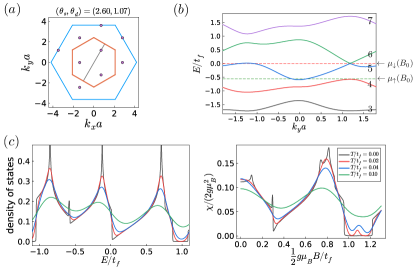
Fig. S5: Model computation using the parameter $(\theta_{s},\theta_{d})=(2.60,1.07)$. (a) Locations of the Dirac nodes in the Brillouin zone (BZ), where blue hexagon is the (original) BZ and the red hexagon is the reduced BZ due to unit-cell tripling. (b) The band spectrum as a function of $k_{y}$ along the parameter cut depicted in gray line in (a) passing through one of the Dirac nodes. In this case, the Dirac nodes are well-defined locally around the Dirac nodes, but there are additional states at $\mu_{\downarrow}(B_{0})$ as well but at different momentum. Also, band 4 and band 5 overlaps in this case, hence $\mu_{\uparrow}(B_{0})$ passes both band 4 and 5. (c) The density of states plot and the magnetic susceptibility plot at zero and finite temperatures. Around $E/t_{f}=0.0$, we see a V-shaped density of states originated from Dirac nodes but now with a finite shift in the $y$-direction due to additional states at $\mu_{\downarrow}(B_{0})$ mentioned in (b). A small peak near $E/t_{f}=\mu_{\uparrow}(B_{0})(\approx 0.6)$ is originated from overlapping band edge contributions from band 4 and 5, which quickly disappear upon introducing finite temperature. As in Fig. S4 (c), there exists two dips in the susceptibility, near $\frac{1}{2}g\mu_{B}B/t_{f}=0.4$ and $\frac{1}{2}g\mu_{B}B/t_{f}=1.1$ responsible for $1/9$ and $1/3$ plateau respectively.

To be concrete, we have constructed a model for fermions hopping on the kagome lattice (for details, see Methods), where $\frac{1}{3}$ of a gauge flux quantum penetrates each unit cell. In addition there are fluxes through the triangles and the hexagon which add up to zero. This choice of gauge flux is motivated by the fact (as seen below) that we need 9 bands per Brillouin zone (BZ) to produce the $\frac{1}{9}$ plateau. Since there are 3 Cu ions per unit cell, we need to triple the unit cell. Without breaking translation symmetry, the $\frac{1}{3}$ gauge flux accomplishes this because in order to describe the gauge potential, the unit cell is necessarily tripled. With a certain choice of parameters, there are three Dirac nodes with velocity $v_{\rm D}$ in the reduced BZ between band 5 and 6, as shown in Fig. 1(b). (In Methods we show that the Dirac node appears along lines in a two dimensional parameter space. Near these lines the Dirac nodes have a small gap. We assume we are in the vicinity these regions. A small gap does not affect our discussion.) Since the spinon carries spin $\frac{1}{2}$, its energy is split by the Zeeman energy $\pm(g/2)\mu_{\rm B}$ where the $g$-factor is close to 2. At zero magnetic field band 5 is half filled to accommodate 9 spinons per unit cell. At field $B=B_{0}$ the down spin chemical potential $\mu_{\downarrow}$ lies at the Dirac point located between band 5 and 6 while the up spin chemical potential $\mu_{\uparrow}$ is in the gap between band 4 and 5. This corresponds to a $\frac{1}{9}$ magnetization plateau. The differential susceptibility $\chi={\rm d}M/{\rm d}H$ is proportional to the DOS $D(\mu)$ and we can expect a linear increase in $\chi$ as $B$ is increased or decreased from $B_{0}$. However, there is a complication in that, as drawn in Fig. 1(b), there is a gap between band 4 and 5. This will give flat bottom in $\chi$ as $\mu_{\uparrow}$ moves across the gap. We assume that this gap is either very small (Fig. S4) or that band 4 and 5 actually overlap (Fig. S5) to eliminate the gap. This will result in a V-shaped $\chi$.

The detailed behavior of $\mu_{\uparrow}$ and $\mu_{\downarrow}$ depends on the DOS $D(\mu_{\uparrow})$ and $D(\mu_{\downarrow})$ and is given in SI section A. Here we mention the key results that $\chi\propto\frac{D(\mu_{\uparrow})D(\mu_{\downarrow})}{D(\mu_{\uparrow})+D(\mu_{\downarrow})}$, namely it is given by the smaller of $D(\mu_{\uparrow})$ and $D(\mu_{\downarrow})$. Thus as long as $\mu_{\downarrow}$ is near the Dirac node where its DOS is small compared to $D(\mu_{\uparrow})$ it will give rise to a V-shaped $\chi$ as seen in the experiment. Since $\mu_{\uparrow}$ is pinned by the larger DOS at the top of band 4, the entire Zeeman splitting goes with $\mu_{\downarrow}$ so that $\mu_{\downarrow}=(g^{\prime}/2)\mu_{B}$ where $g^{\prime}\approx 2g$. We remark that the up-spin Fermi surfaces can also exhibit quantum oscillations (See SI section D) and will dominate the heat capacity which is predicted to be linear in $T$.

Next we address the question of quantum oscillations. For $kT<<\mu_{\downarrow}$ we show that the oscillatory part of the torque $\tau$ is given approximately by (for details see SI section C)

$$\frac{\tau}{BL^{2}}=\textup{sin}\theta C_{0}(B-B_{0})\frac{aT}{\sinh{aT}}{\textup{sin}}(2\pi\frac{(B-B_{0})^{2}}{B\cdot\Delta B}+\varphi).$$ (1)

Here, $C_{0}=\frac{2e}{\pi^{2}\hbar}$ and the oscillation in the last term is parametrized by

$$\Delta B=2e\hbar\frac{\alpha v_{D}^{2}}{((g^{\prime}/2)\mu_{B})^{2}}\rm{cos}\theta.$$ (2)

The $(B-B_{0})^{2}$ factor inside the sine in Eq. 1 originates from $\mu_{\downarrow}$. We see that for $B$ large compared to $B_{0}$, the quantum oscillations are roughly periodic in $B$ with period $\Delta B$. More generally, the Landau Level quantization goes as $n\approx\frac{(B-B_{0})^{2}}{B\Delta B}$. This is shown to be consistent with the experimental data in the Landau-Level-index plots of Fig. 3(b).

Fig. 3(c) displays the resulting $\Delta B$ for all the measured tilt angles. Despite very little angular dependence of the field $B_{0}$ (shown in the insert), the period $\Delta B$ drops by more than a factor of 5, following closely the $\cos(\theta)$ dependence predicted by Eq. 2. This is a strong indication that the oscillations depend on the component of the magnetic field along $c$, and that they have an orbital origin. This is quite remarkable considering the system is described by a spin model without a significant orbital degree of freedom.

In Eq. 1 the temperature dependence is given by the LK form $\frac{aT}{\sinh{aT}}$ which we parametrize in terms of the standard two-dimensional (2D) LK form for a parabolic band with mass $m^{*}$, i.e. $a=\frac{2\pi^{2}}{e\hbar}\frac{m^{*}}{Bcos(\theta)}$. For our problem the effective mass is given by

$$\frac{m^{*}}{m_{e}}=\frac{(g^{\prime}/2)\mu_{B}(B-B_{0})}{\alpha v_{D}^{2}m_{e}}.$$ (3)

Note that this is independent of the angle $\theta$ and proportional to $B-B_{0}$. Therefore the oscillations tend to be more suppressed by temperature for increasing $B$. On the other hand, the linear term in $B-B_{0}$ in front of Eq. 1 suppresses the low field oscillations, resulting in a maximum in the oscillation envelope for intermediate $B$.

There is a simple relationship between $\Delta B$ and $m^{*}/m_{e}$

$$\frac{m^{*}}{m_{e}}\Delta B=4\frac{g}{g^{\prime}}(B-B_{0})\cos\theta.$$ (4)

From Fig. 3(c), $\Delta B/\cos(\theta)=3.46$ T. Putting this into Eq. 4 and using $g^{\prime}=2g$ and $B-B_{0}=10$ T, we find $m^{*}/m=5.78$. This is in reasonable agreement with the measured value 3.7 shown in Fig. 2. The prediction that $m^{*}$ increases with increasing $B$ as $B-B_{0}$ is also in rough agreement with the LK fit of the amplitude shown in Fig. S7. The relationship between $m^{*}$ and $\Delta B$ lies at the heart of the fermionic model with Landau level quantization; its validity provides key support for this picture.

We can also use Eq. 2 to extract the Dirac velocity $v_{\rm D}$. Taking $g^{\prime}=2g\approx 4$ we find $\sqrt{\alpha}v_{\rm D}\approx 39~{}$meV$\cdot$Å$\approx 5.89\times 10^{3}$ m/sec. The velocity is also extracted from the slope of $\chi$ vs $B$ in SI section E, yielding $v_{\rm D}\approx 34~{}$meV$\cdot$Å. This estimate strongly depends on the number of Dirac nodes but nevertheless suggests that $\alpha$ is not far from unity. On the other hand, in the spinon model, we estimate $v_{\rm D}\approx 11~{}$meV$\cdot$Å which is considerably smaller (Methods). Note that strong interactions between spinons can lead to an upward renormalization of the quasiparticle velocity Son2007 ; Geim which is what is measured via quantum oscillations, while the magnetic susceptibility is a response function which is renormalized differently.

In SI section F we show that $\alpha$ does not have to be much smaller than unity even when the charge gap is relatively large. Subject to these large uncertainties, the values of $v_{\rm D}$ and $\alpha$ derived from the data are reasonably consistent.

We note that this paper deals with the high field region near the $\frac{1}{9}$ plateau and does not address the question of whether a Dirac spin liquid exists at zero field Zeng2022 ; Zeng2023 . The current phenomenological model breaks time-reversal symmetry which is natural in the presence of a large magnetic field but not in zero field. More importantly, in the current model at zero field, band 5 is half filled, resulting in a spinon Fermi surface. In order to have a Dirac spin liquid at zero field, we need to double the unit cell, as was done in Ran2007 ; Hermele2008 . Therefore the state we propose is not expected to survive to low magnetic fields.

In summary, magnetic quantum oscillations are observed in the magnetic torque of the kagome AFM Mott insulator YCu3-Br, and well reproduced in several samples (Fig. S10). These oscillations are unconventional in the following senses. (1) The oscillations are roughly periodic in large applied fields $B$. (2) Their period, $\Delta B$, follows a $\cos\theta$ dependence, suggesting that they are caused by an orbital effect. (3) The $T$ dependence of the oscillation amplitude follows the LK formula, expected for fermions. As discussed above, a Dirac fermion model that emerges near the $\frac{1}{9}$ plateau explains all three observations. Furthermore the mass parameter extracted using the LK model is consistent with the oscillation period, verifying the key relation given by Eq. 4. These observations provide strong support for the observation of fractionalized fermions coupled to an emergent gauge field. A Dirac spinon model located at the $\frac{1}{9}$ plateau can account for much of the data. At this point the model is phenomenological and serves an interim purpose to organize the data. We have not addressed how it can be derived from a microscopic model of the kagome Heisenberg spin system. It is not known whether the disorder introduced by the random occupation of the Br sites by OH plays a role Liu2022 . The role of the DM term is also not clear. Obviously there is much room for further theoretical work.

Acknowledgement This work is supported by the National Science Foundation under Award No. DMR-2004288 (transport measurements), by the Department of Energy under Award No. DE-SC0020184 (magnetization measurements). A portion of this work was performed at the National High Magnetic Field Laboratory (NHMFL), which is supported by National Science Foundation Cooperative Agreement Nos. DMR-1644779 and DMR-2128556 and the Department of Energy (DOE). J.S. acknowledges support from the DOE BES program “Science at 100 T,” which permitted the design and construction of much of the specialized equipment used in the high-field studies. The work at IOP China is supported by the National Key Research and Development Program of China (Grants 2022YFA1403400, No. 2021YFA1400401), the K. C. Wong Education Foundation (Grants No. GJTD-2020-01), the Strategic Priority Research Program (B) of the Chinese Academy of Sciences (Grants No. XDB33000000). The experiment in NHMFL is funded in part by a QuantEmX grant from ICAM and the Gordon and Betty Moore Foundation through Grant No. GBMF5305 to Kuan-Wen Chen, Dechen Zhang, Guoxin Zheng, Aaron Chan, Yuan Zhu, and Kaila Jenkins. P.L. acknowledges the support by DOE office of Basic Sciences Grant No. DE-FG02-03ER46076 (theory).

$\dagger$These authors contributed equally and shared the first authorship.

Methods

Experimental Details

Single crystals of $\text{YCu}_{3}(\text{OH})_{6}\text{Br}_{2}[\text{Br}_{x}(\text{OH})_{1-x}]$ (YCu3-Br) were grown using the hydrothermal method and ultrasonically cleaned in water before measurements to remove the possible impurities as reported previously Schulenburg2002 ; Zeng2022 . The deuterated single crystals (YCu3-D-Br) were synthesized using the same method with the corresponding deuterated starting materials and heavy water. The Cl-doped single crystals (YCu3-(Br, Cl)) were synthesized using the same method as YCu3-Br with 10$\%$ Br atoms replaced by Cl atoms.

Magnetization measurements at low field ($<$ 14 T) were carried out in a Quantum Design physical property measurement system (PPMS Dynacool-14T) using the Vibrating Sample Magnetometer (VSM) option.

Magnetization measurements at high field were using a compensated-coil spectrometer Goddard2007 ; Goddard2008 as drawn in Fig. S6(a) which were performed at 65 T and 73 T pulsed field magnet at the National High Magnetic Field Laboratory (NHMFL), Los Alamos.

Magnetic torque measurements on YCu3-Br S1, S2, and YCu3-D-Br S2 were using a piezo-resistive cantilever as drawn in Fig. 2(b) performed in 41 T Cell 6 and 45 T Hybrid DC field magnets in NHMFL, Tallahassee, the ignorable unloaded cantilever setup signals are measured in PPMS as shown in Fig. S1.

Magnetic torque measurements on YCu3-Br S3 were using a membrane-type surface-stress sensor as shown in Fig. S6(c) performed in 73 T pulsed field magnet in NHMFL, Los Alamos.

Magnetic torque measurements on YCu3-D-Br S1 were using a capacitive cantilever as drawn in Fig. S10(b) performed in 41 T Cell 6 DC field magnets in NHMFL, Tallahassee.

Effective spinon model

In this section, we introduce a mean-field Hamiltonian which is used as an effective description for YCu3-Br. As briefly mentioned in the main text, the mean-field Hamiltonian is a tight-binding model of nearest-neighbor hopping of spinons, which is coupled to an internal gauge field. The Hamiltonian is given by

$$H_{\rm MF}= - \sum_{\langle i,j\rangle,\sigma}\big{(}t_{f}e^{iA_{i,j}}c_{i,\sigma}^{\dagger}c_{j,\sigma}+{\rm h.c.}\big{)}$$ (5)

$$- \sum_{i,\sigma}\big{(}\mu-\sigma\frac{1}{2}g\mu_{B}B\big{)}c_{i,\sigma}^{\dagger}c_{i,\sigma},$$

where $A_{i,j}$ is the internal gauge field coupled with the spinons, $t_{f}$ is the hopping strength which is proportional to the antiferromagnetic coupling $J$ in the bare Hamiltonian, $\sigma=$ $\uparrow$ ($+1$) and $\downarrow$ ($-1$) denote spin-up and spin-down spinons, $\mu$ is the chemical potential, B is the strength of the external magnetic field, $g$ is the g-factor of spinon, and $\mu_{B}$ is the Bohr magneton.

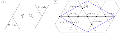
Fig. S2: Gauge flux configuration and filed configurations. (a) Flux pattern of a spontaneously generated internal gauge field in the kagome lattice, which is independent of the external magnetic field $B$. The flux pattern is parametrized by two angles $\theta_{s}$ and $\theta_{d}$, where $\theta_{s}$ is the averaged flux of two triangles and $\theta_{d}$ measures the flux difference between upward triangle and downward triangle. By summing up the fluxes in the usual kagome unit-cell we have $2\pi/3$ flux in total, implying that the unit-cell has to be tripled. (b) Our choice of a tripled unit-cell denoted as a blue rhombus together with the gauge configuration realizing the flux pattern in (a). Only the gauge configuration relevant to the sites in the tripled unit-cell is shown and lines without the arrow corresponds to zero gauge field configuration.

Several remarks are in order. The internal gauge field is a sum of two contributions—one is a spontaneously generated internal gauge field resulting in the flux pattern described in Fig. S2 (a) and the other is the induced gauge field due to the $c$ component of physical magnetic field via the Ioffe-Larkin relation Lee06 ; Inti22 with the proportionality constant $\alpha$ as explained in Eq. 34. The spontaneously generated fluxes are parameterized by two angles $\theta_{s}$ and $\theta_{d}$ are defined in Fig. S2 (a), where $\theta_{s}$ measures the average flux between two triangles and $\theta_{d}$ measures flux difference between two triangles. $\theta_{s}$ can be generated from the Dzyaloshinskii-Moriya (DM) type of interactions Lee06 ; gao2020 . However, its magnitude is expected to be small, being proportion to the ratio of the DM interaction to the exchange term J, multiplied by the magnetization in units of $\mu_{B}$ which is  1/9. On the other hand, $\theta_{d}$ is generated by a term that breaks $C_{6}$ symmetry into $C_{3}$. We also note that since the spinon is a fractionalized particle, the chemical potential $\mu$ is tuned to satisfy the mean-field filling constraint $\sum_{i}\big{(}\sum_{\sigma}\langle c_{i,\sigma}^{\dagger}c_{i,\sigma}\rangle-1\big{)}=0$ and will have $B$ dependence, as treated in detail in the next section. It will prove to be useful to introduce the chemical potential for the up-spin $\mu_{\uparrow}(B)=\mu-\frac{1}{2}g\mu_{B}B$ and the chemical potential for the down-spin $\mu_{\downarrow}(B)=\mu+\frac{1}{2}g\mu_{B}B$, where the dependence of $\mu$ in $B$ is implicit.

Due to background $2\pi/3$ flux depicted in Fig. S2 (a), the unit cell of Eq. 5 is tripled compared to the usual unit cell of the kagome lattice. The mean-field Hamiltonian contains two variational parameters $\theta_{s}$ and $\theta_{d}$, which controls the strength of the magnetic flux of hexagon and triangles. For generic $\theta_{s}$ and $\theta_{d}$, the effective Hamiltonian has the $C_{3}$ symmetry with the rotation center being the center of a hexagon. While the flux pattern is invariant under the spatial $\pi/3$-degree rotation, the gauge field configuration is invariant only when it is followed by an additional gauge transformation. Due to this additional gauge transformation, the Hamiltonian at momentum $\bm{k}$ is not related to the Hamiltonian at $R(\pi/3)\bm{k}$, where $R(\pi/3)$ is the $\pi/3$-degree rotation matrix, but rather related to the Hamiltonian at $R(\pi/3)\bm{k}+\bm{k_{a}}$, where $\bm{k_{a}}$ is set by the additional gauge transformation and hence is an artifact of our choice of the gauge field configuration realizing the flux pattern. This can be seen at the locations of the Dirac nodes in Fig. S4 (a), where we have three Dirac nodes come in triple due to the $C_{3}$ symmetry, but the center of three nodes are shifted away from the $\Gamma$ point in the reduced Brillouin zone. This shift depends on the gauge choice $\bm{k_{a}}$ and is not physical. Also, the effective Hamiltonian is invariant under the shift $(\theta_{s},\theta_{d})\to(\theta_{s}+\pi,\theta_{d}+\pi)$ and the inversion symmetry, followed by a gauge transformation, maps the Hamiltonian for $(\theta_{s},\theta_{d})$ to the Hamiltonian for $(\theta_{s},-\theta_{d})$.

When the external magnetic field $B$ is zero, $\mu_{\uparrow}$ and $\mu_{\downarrow}$ are identical, we therefore have $4.5$ filling per tripled unit cell set by the filling constraint. Then upon turning on the external magnetic field, we occupy more spin-down spinon than spin-up spinon, where the difference in the chemical potential is given by $g\mu_{B}B$. We are mainly interested in the regime where spin-down spinon fully occupies the $5$th band and is describes by a Dirac particle. This happens when the 5th band and the 6th band touches with each other and the band touchings are described by Dirac nodes as in Figs. S4 and S5.

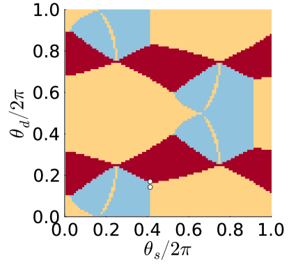
Fig. S3: The ground state Chern number over the parameter space. The Chern number of the occupied states over the parameter space $(\theta_{s},\theta_{d})$ assuming the band is filled up to the 5th band. The Chern number $C=1$ region is colored in yellow and $C=2$ is colored in blue. The red region corresponds to the case where there is no band gap between the 5th and the 6th band, hence the Chern number is not well-defined. Using symmetries, we see that the entire region is just a tiling of a quarter of the region $0\leq\theta_{s}/2\pi,\theta_{d}/2\pi\leq 0.5$, so we only need to focus on this 1/4 region. Two white dots located along the vertical cut $\theta_{s}/2\pi\approx 0.4$ in the figure are two parameters studied in Figs. S4 and S5, where we have three Dirac nodes between the 5th and the 6th band together with a small or no gap between the 4th band and the 5th. While we have three Dirac nodes whenever the parameter $(\theta_{s},\theta_{d})$ is located at the common boundary between $C=2$ and $C=-1$ region, many of them have rather a large gap between band 4 and 5. A small crescent-shaped $C=1$ island emanating from $(\theta_{s}/2\pi,\theta_{d}/2\pi)\approx(0.2,0.0)$ inside a $C=2$ region has very flat 5th and 6th band, so that the $C=1$ region spans over a small parameter range.

While there is a band gap between the $5$th band and the $6$th band over a wide range of the parameter space $\theta_{s}$ and $\theta_{d}$, there are special lines along which two bands are gapless with three Dirac nodes. In Fig. S3, we computed the Chern number of the ground state assuming that the chemical potential is located in the gap between the 5th band and 6th band. [Here, we only consider one of the spin component in Eq. 5.] We first note that we only need to consider a quarter of the entire region, e.g., $0\leq\theta_{s},\theta_{d}\leq\pi$. This can be shown by utilizing the facts that the Hamiltonian is invariant under the shift $(\theta_{s},\theta_{d})\to(\theta_{s}+\pi,\theta_{d}+\pi)$ and that although the inversion symmetry is not the symmetry of the Hamiltonian, but it maps $(\theta_{s},\theta_{d})$ to $(\theta_{s},-\theta_{d})$ while preserving the Chern number. The red region in Fig. S3 is the region where there is no gap between band 5 and 6 so that the Chern number is not well-defined. The blue region highlights the region where the Chern number $C$ equals $2$ and the yellow region is the region where $C=-1$. The common boundaries between $C=2$ region and $C=-1$ region give the parameter lines along which we have three Dirac nodes between band 5 and 6. We also note that the difference in the Chern number $\Delta C=3$ between two regions is precisely captured by three Dirac nodes.

In the following, we assume that the band touchings between the 5th band and the 6th band are described by three Dirac nodes, although most of the following discussions still hold even when the Dirac nodes are gapped out with a small gap. In particular, we focus on two points in the parameter space indicated as two dots in Fig. S3 located at the vertical cut along $\theta_{s}/2\pi\approx 0.4$. We have chosen these two points because here there gap between band 4 and band 5 is small. Together with the presence of the Dirac nodes between band 5 and 6, We will see in the following section that it is important to have a small or no gap between band 4 and 5 in order to have a V shaped differential spin susceptibility. This will also lead to an enhanced $g$ factor for spin-down particle due to the $B$ dependence of $\mu$ (see next section) and hence most relevant for our experiment.

In Fig. S4, we used $(\theta_{s},\theta_{d})=(2.60,0.90)$ as our parameters for fluxes and computed (a) the locations of the Dirac nodes between the band 5 and 6, (b) band structure along the cut in the reduced Brillouin zone described in (a), and (c) the density of states and the susceptibility as a function of the external magnetic field. There are three Dirac nodes exist in the reduced Brillouin zone which results in V-shaped density of states around $\mu_{\downarrow}(B_{0})$. From the zero temperature density of states, one can compute the temperature smearing effect in the density of states using

$$D_{T}(\epsilon)=-\int_{-\infty}^{\infty}\frac{\partial f_{\rm F-D}(\epsilon^{\prime}-\epsilon)}{\partial\epsilon^{\prime}}D(\epsilon^{\prime})d\epsilon^{\prime},$$ (6)

where $f_{\rm F-D}$ is the Fermi-Dirac distribution, and can compute the magnetic susceptibility using Eq. 20. As clearly can be seen from finite temperature curves of the susceptibility plot, there are two dips around $\frac{1}{2}g\mu_{B}B/t_{f}\approx 0.4$ and $1.1$, which are responsible for $1/9$ and $1/3$ plateau observed in the experiment. Using the fact that $1/9$ dip forms at $B_{0}\approx 20T$, it gives an estimated value for $t_{f}\approx 2.9\textrm{ meV}$. Using the value of $J$ discussed in the text we estimate $t_{f}/J\approx 1/2$ which is reasonable because the mean field hopping parameter for spinon is expected to be reduced from $J$. Moreover, the estimated $t_{f}$ gives $T=3.4\textrm{ K}$ for $T/t_{f}=0.1$, which is consistent with the temperature scale observed in the experiment by comparing $T/t_{f}=0.1$ (green) curves in Fig. S4 (c) and Fig. S5 (c) with $T=3.0\textrm{ K}$ curves in Fig. S9 (a) from the experiment.

We can also estimate the Dirac velocity by noting that the typical value in the cases shown in Fig S4 is given by $0.55\ t_{f}a/\hbar$ where $a=6.68\AA$ is the lattice constant. This gives a value of about $11meV\cdot\AA$.

We note that the finite Chern number of the band below the Dirac nodes mean that this model predicts edge modes and quantized anomalous thermal conductivity. On the other hand, the Dirac nodes co-exists with a Fermi surface for the up spin spinons. Spin SU(2) symmetry is broken by the DM term and time reversal is explicitly broken. Admixture between up and down spin will delocalize these edge modes. We still expect a metal-like thermal conductivity together with a metal-like linear $T$ specific heat in this phenomenological model.

FFT analysis of magnetic oscillations

In order to conduct FFT analysis on the oscillatory features, we performed a Loess smooth background subtraction on the torque derivative data, as shown in Fig. S7(b); the subtracted temperature dependence of magnetic oscillations is shown in Fig. S7(c) top panel. Next, we rescaled the $x$ axis of Fig. S7(c) from $B$ to $(B-B_{0})^{2}/B$ in order to get periodic patterns along $x$ axis, as shown in the inset of Fig. S7(e). Fig. S7(e) are the corresponding FFT spectra at different temperatures using a transform window from 24.0 T to 35.7 T. We can see there is a dominant frequency around 0.35 T^-1, which corresponds to our defined period $\Delta B\sim 2.86$ T at -38.3^∘, and the amplitudes of dominant frequency at different temperatures are plotted in Fig. 2(d). We also notice that the frequency becomes slightly smaller with increasing temperature; one possible reason is the linear energy dispersion induced frequency shift at different temperatures Guo2021 . We emphasize that the mass obtained by LK fitting $aT/\mathrm{sinh}(aT)$ in Fig. 2(d) is the averaged effective mass over the FFT window; in fact $m^{*}$ is field-dependent. Therefore, we also show the amplitude of each peak and valley of Fig. S7(c) data at fixed field in Fig. S7(d), and find $m^{*}$ by performing LK fits shown in the inset of (d). The increasing trend of $m^{*}$ with magnetic field is roughly consistent with Eq. 3.

Supplemental Figures

Fig. S1: Background signal of empty cantilever setup. The torque signals of empty cantilever versus $H$ field compared with the same cantilever setup loaded with YCu3-Br S1 sample measured in PPMS at different angles. The empty cantilever signals are small enough and do not have angular dependence compared with the cantilever loaded with sample.

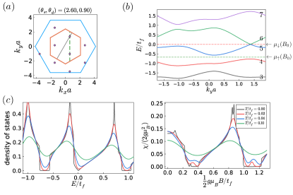
Fig. S4: Model computation using the parameter $(\theta_{s},\theta_{d})=(2.60,0.90)$. (a) Locations of the Dirac nodes in the Brillouin zone (BZ), where blue hexagon is the (original) BZ and the red hexagon is the reduced BZ due to unit-cell tripling. Vertical dashed line is a momentum cut used in the band spectrum plot Fig. 1 (b). (b) The band spectrum as a function of $k_{y}$ along the parameter cut depicted in gray line in (a) passing through one of the Dirac nodes. At critical magnetic field $B=B_{0}$, the down-spin chemical potential $\mu_{\downarrow}(B_{0})$ is located at the Dirac node and the up-spin chemical potential $\mu_{\uparrow}(B_{0})$ is located in between the band 4 and band 5. (c) The density of states plot and the magnetic susceptibility plot at zero and finite temperatures. Around $E/t_{f}=0.0$, we see a V-shaped density of states originated from Dirac nodes. At zero temperature, we see a vanishing density of states near $E/t_{f}=0.7$ ($E/t_{f}=1.0$), due to the band gap between band 4 and 5 (band 6 and 7). Although the density of states vanishes whenever there is a band gap in the theory calculation, we expect the density of states actually does not vanish in the real material due to the presence of in-gap modes from disorder. These small density of states give two dips in the susceptibility, near $\frac{1}{2}g\mu_{B}B/t_{f}=0.4$ and $\frac{1}{2}g\mu_{B}B/t_{f}=1.1$ responsible for $1/9$ and $1/3$ plateau respectively.

Fig. S6: Temperature dependence of high field measurements. (a) Temperature dependence of static Magnetization versus field of YCu3-Br sample M measured in pulse magnetic field with $H\parallel c$. Inset: experimental setup of a compensated coil magnetometer for magnetization measurements in pulse magnetic field. The compensated coils are shown in dark blue (1000 turns) and light blue (500 turns in the other direction). The samples were stacked in a non-magnetic tube and inserted into the coil. (b) Temperature dependence of magnetization versus field of YCu3-(Br, Cl) measured in pulse magnetic field with $H\parallel c$. Both 1/9 and 1/3 plateaus in magnetization were observed at temperatures $<4.2$ K. (c) Temperature dependence of magnetic torque versus field of YCu3-Br S3 in pulse field using a surface-stress sensor (picture in inset) at $\theta=23.8^{\circ}$. (d) Derivative of Magnetization $dM/dH$ versus field of YCu3-(Br, Cl) in (b). The yellow line around 18 T is the linear fitting to obtain the slope $k_{\chi}$ in the vicinity of $B_{0}$. The inset shows the slope $k_{\chi}$ at multiple temperatures. The blue curve represents the result of Fermi-Dirac smearing performed on the $T=0.5$ K data set assuming $g^{\prime}=2g.$

Fig. S7: Detailed analysis of torque measurements in YCu3-Br S1. (a) Angular dependence of magnetic torque versus field of YCu3-Br S1 measured in a 41 T resistive magnet. (b) Torque derivative $d\tau/dH$ versus field with dashed curves showing the background for subtraction at $\theta=-38.3^{\circ}$ and $87.8^{\circ}$. The background was obtained by performing Loess smooth on the data, then subtracted to obtain the oscillation component. (c) Top panel is the oscillation component isolated from $d\tau/dH$ after background subtraction at $\theta=-38.3^{\circ}$ at different temperatures, and bottom panel is the temperature smeared results by using Eq. 23 which takes the 0.4 K oscillation data as convolution data and set $g^{\prime}=2g$. (d) The normalized amplitude of oscillation extremas versus temperature at fixed field at $\theta=-38.3^{\circ}$. An offset was added to the plots for clarity. The LK fitting are shown in solid lines. Inset: effective mass $m^{*}$ obtained from the LK fitting function. (e) The FFT analysis at different $T$, obtained from the inset periodic oscillations. The peak location of FFT is the frequency of oscillations, which is $1/\Delta B$. The FFT range is from 24.0 T to 35.7 T. (f) Conventional Landau plot at two angles to check the oscillations are not periodic in $1/B$.

Fig. S8: Angular dependence of Landau level plots in YCu3-Br S1. Top panel: Black curves are $d^{2}\tau/dH^{2}$ measured at 0.4 K, red curves are the corresponding oscillations after background subtraction. “$\times 3$” means the oscillation amplitudes are increased by 3 for clarity. Bottom panel: Landau index plots of the $d^{2}\tau/dH^{2}$ amplitudes. Solid curves are the fitting results of $n=(B-B_{0})^{2}/(\Delta B\cdot B)+\phi$.

Fig. S9: Temperature dependence of -14.1^∘ and 87.8^∘ data in YCu3-Br S1. (a) (d) Top panel: the measured torque data up to 40 T at different $T$. Bottom panel: the corresponding $d\tau/dH$ plots. (b) (e) are the corresponding $d^{2}\tau/dH^{2}$ plots. The sharp dips in (e) around 32 T may indicate a phase transition. (c) (f) LK fitting of normalized FFT amplitudes of $d\tau/dH$ oscillations. The resulting average effective mass for -14.1^∘ is $5.1\ m_{e}$ which is similar to the value 3.7$\ m_{e}$ found in Fig. 2(d) at -38.3^∘. On the other hand, for 87.8^∘ the effective mass is much smaller, $\approx 0.42\ m_{e}$. We note that at $\theta=$87.8^∘, cos$\theta$ and $B_{c}$ are very small and a small effective mass is indeed needed to give an observable signal at a reasonable temperature. It is possible that oscillations at angles very close to 90^∘ is of a different origin and require further studies. Inset: FFT analysis (See Methods). The FFT window in (c) is [22.4 T, 36.9 T], and the FFT window in (f) is [23.2 T, 30.8 T].

Fig. S10: Magnetic torque measured with different samples. (a) Magnetic torque of YCu3-Br sample S2 measured using piezoresistive cantilever in hybrid magnet from 11.5 to 42.5 T at multiple temperatures. The data is in good agreement with YCu3-Br sample S1 measured in resistive magnet. (b) Magnetic torque of YCu3-D-Br sample S1 measured using capacitive cantilever in a resistive magnet up to 41 T at different temperatures. Inset shows the experimental setup of the capacitive cantilever. (c) Comparison of $d^{2}\tau/dH^{2}$ versus magnetic field for different samples. The measurement and growth conditions of each sample can be found in Methods. The wiggles are reproducible in different samples using different methods of measurement.

Supplementary Information

.1 Chemical potential of up and down spin fermions and their temperature smearing

Here, we start from spin-1/2 Hamiltonian induced by an applied magnetic field:

$$H_{B} =-g\mu_{B}\vec{S}\cdot\vec{B}$$

$$=\begin{cases}+\frac{1}{2}g\mu_{B}B,\ \rm{for\ up}(\uparrow)\ \rm{spin}\\ -\frac{1}{2}g\mu_{B}B,\ \rm{for\ down}(\downarrow)\ \rm{spin}\end{cases}$$ (7)

The energy for up spin is $\epsilon_{\uparrow}-\mu=\epsilon+\frac{1}{2}g\mu_{B}B-\mu=\epsilon-\mu_{\uparrow}$. Here $\epsilon$ is the energy of spinor without magnetic field, and $\mu$ is the chemical potential, and we define the chemical potential for up spin is $\mu_{\uparrow}=\mu-\frac{1}{2}g\mu_{B}B$. Similarly, the energy for down spin is $\epsilon_{\downarrow}-\mu=\epsilon-\mu_{\downarrow}$, where $\mu_{\downarrow}=\mu+\frac{1}{2}g\mu_{B}B$. Here $\mu$ should depend on field B in order to satisfy the constraint $n_{\uparrow}+n_{\downarrow}=const.$, and $n_{\uparrow}$ ($n_{\downarrow}$) is the number of up (down) spins. Start from the definition of $n_{\downarrow}$,

$$n_{\downarrow}=\int f_{\rm{F}-\rm{D}}(\epsilon-\mu_{\downarrow})D(\epsilon)d\epsilon$$ (8)

Here $f_{\rm{F}-\rm{D}}$ is the Fermi-Dirac distribution function. Then,

$$\frac{dn_{\downarrow}}{dB}=-\int\frac{\partial f_{\rm{F}-\rm{D}}(\epsilon-\mu_{\downarrow})}{\partial\epsilon}(\frac{d\mu}{dB}+\frac{1}{2}g\mu_{B})D(\epsilon)d\epsilon$$ (9)

When $k_{B}T\ll\mu$,

$$\frac{dn_{\downarrow}}{dB}=(\frac{d\mu}{dB}+\frac{1}{2}g\mu_{B})D(\mu_{\downarrow})$$ (10)

Similarly, we find

$$\frac{dn_{\uparrow}}{dB}=(\frac{d\mu}{dB}-\frac{1}{2}g\mu_{B})D(\mu_{\uparrow})$$ (11)

Combining equations above, we obtain

$$\frac{d\mu}{dB}=\frac{1}{2}g\mu_{B}\frac{D(\mu_{\uparrow})-D(\mu_{\downarrow})}{D(\mu_{\uparrow})+D(\mu_{\downarrow})}$$ (12)

Therefore, we have

$$\frac{d\mu_{\downarrow}}{dB}=\frac{1}{2}g\mu_{B}\frac{2D(\mu_{\uparrow})}{D(\mu_{\uparrow})+D(\mu_{\uparrow})}$$ (13)

We assume that band 5 and 6 overlap so that $\mu_{\uparrow}$ lies in the band and $D(\mu_{\uparrow})$ has a finite value. On the other hand, when $B$ is near $B_{0}$, $\mu_{\downarrow}$ is near the Dirac point, $D(\mu_{\downarrow})$ is much smaller than $D(\mu_{\uparrow})$. The RHS of Eq. 13 is approximately constant and we integrate Eq. 13 obtain

$$\mu_{\downarrow}=\frac{1}{2}g^{\prime}\mu_{B}(B-B_{0}).$$ (14)

where we define the effective g factor as

$$g^{\prime}=(1+\frac{D(\mu_{\uparrow})}{D(\mu_{\uparrow})+D(\mu_{\downarrow})})g$$ (15)

Near the Dirac point, $D(\mu_{\downarrow})<<D(\mu_{\uparrow})$, $g^{\prime}\approx 2g$ and $\mu_{\downarrow}$ moves twice as fast as $\frac{1}{2}g\mu_{B}B$.

We next derive the expression for $\mu_{\uparrow}$. Using Eq. 12 we find

$$\frac{d\mu_{\uparrow}}{dB}=\frac{1}{2}g\mu_{B}\frac{2D(\mu_{\downarrow})}{D(\mu_{\uparrow})+D(\mu_{\uparrow})}$$ (16)

As before we assume $\mu_{\uparrow}$ lies near the top of band 5 and/or the bottom of band 6, so $D(\mu_{\uparrow})$ is large than $D(\mu_{\downarrow})$ which lies near the Dirac node. It is given by $D(E)=\nu|E|$ where $\nu=M_{\downarrow}/2\pi v_{D}^{2}$ and $M_{\downarrow}$ is the number of Dirac nodes. Setting $D(\mu_{\downarrow})=D(E=(g^{\prime}/2)\mu_{B}(B-B_{0}))$ and integrating Eq. 16, we find

$$\mu_{\uparrow}=(g^{\prime}/2)(g/2)\mu_{B}^{2}4\nu(B-B_{0})^{2}/D(\mu_{\uparrow})$$ (17)

The important point is that $\mu_{\uparrow}$ moves slowly as $(B-B_{0})^{2}$. We will make use of this in a later section on the quantum oscillation from the up spin Fermi surface.

Next we derive the temperature smearing effect in magnetic properties. Starting from Eq. 9, we can define

$$\tilde{D}(\mu_{\downarrow(\uparrow)})=-\int\frac{\partial f_{\rm{F}-\rm{D}}(\epsilon-\mu_{\downarrow(\uparrow)})}{\partial\epsilon}D(\epsilon)d\epsilon$$ (18)

At zero temperature $\tilde{D}(\mu_{\downarrow(\uparrow)})$ goes to ${D}(\mu_{\downarrow(\uparrow)})$. The definition of magnetic susceptibility is related to the imbalanced numbers between up and down spins:

$$\chi =\mu_{B}(\frac{dn_{\downarrow}}{dB}-\frac{dn_{\uparrow}}{dB})$$ (19)

$$=\frac{1}{2}g\mu_{B}^{2}\frac{4\tilde{D}(\mu_{\downarrow})\tilde{D}(\mu_{\uparrow})}{\tilde{D}(\mu_{\downarrow})+\tilde{D}(\mu{\uparrow})}$$ (20)

When $\mu_{\downarrow}$ is close to the Dirac point, $\tilde{D}(\mu_{\downarrow})<<\tilde{D}(\mu_{\uparrow})$ , so

$$\chi\approx 2g\mu_{B}^{2}\tilde{D}(\mu_{\downarrow})$$ (21)

In the $T\to 0$ limit, $\chi_{0}\equiv\chi(T=0)\approx 2g\mu_{B}^{2}D(\mu_{\downarrow})$ and show the V shape dip. At finite $T$:

$$\chi(T)=-\int\frac{\partial f_{\rm{F}-\rm{D}}(\epsilon-\mu_{\downarrow})}{\partial\epsilon}\chi_{0}(\epsilon)d\epsilon$$ (22)

After plugging $\epsilon=\frac{1}{2}g^{\prime}\mu_{B}(B^{\prime}-B_{c})$ and $\mu_{\downarrow}=\frac{1}{2}g^{\prime}\mu_{B}(B-B_{0})$ into Eq. 22, we obtain

$$\chi(T,B) =-\int\frac{\partial f_{\rm{F}-\rm{D}}[\frac{1}{2}g^{\prime}\mu_{B}(B^{\prime}-B)]}{\partial B^{\prime}}\chi_{0}(B^{\prime})dB^{\prime}$$ (23)

Eq. 23 is the final equation we got to study the temperature smearing effect. Around Dirac point $B=B_{0}$, we can take $g^{\prime}=2g$. Fig. 2(c) and Fig. S6(d) are the smearing results we got by using Eq. 23 and taking $g^{\prime}=2g$.

.2 Model of the quantum oscillations of the field-driven Fermi surfaces of Dirac fermions

Here, we use a simple model to describe the quantum oscillations of the Dirac fermions in the U(1)-Dirac spin liquid state under the magnetic field. The energy dispersion of two-component Dirac fermions can be described by the equation $E(\textbf{k})=\hbar v_{D}k$, and $v_{D}$ is the Fermi velocity. After applying the magnetic field, the chemical potential $\mu$ will split as $\mu_{\downarrow(\uparrow)}=Sg^{\prime}\mu_{B}(\pm B-B_{0})$ due to the Zeeman effect. Here $S=1/2$, and $g$-factor is around 2 in the YCu3-Br. We assume the down spins will approach the Dirac point at $B=B_{0}$, so in the following derivation we mainly focus on the energy of down spins. Therefore, we can set $\mu_{\downarrow}=\frac{1}{2}g^{\prime}\mu_{B}(B-B_{0})=E_{F}$ to get the expression of Fermi wavelength $k_{F}$:

$$k_{F}=\frac{g^{\prime}\mu_{B}}{2\hbar v_{D}}(B-B_{0})$$ (24)

Next we consider the Landau level quantization of Dirac fermions under the magnetic field. Assume spinors see gauge magnetic field $b=\alpha B\rm{cos}\theta$. When $\mu_{B}B>>\Delta E_{L}$ where $\Delta E_{L}$ is the energy of Landau level spacing, we can use Bohr-Sommerfeld semiclassical quantization Shoenberg :

$$\frac{eb_{n}(n+\gamma)}{\hbar}=\frac{A_{F}}{2\pi}$$ (25)

Here $b_{n}$ is the gauge field when $n$th Landau level crosses Fermi energy, and $0\leq\gamma<1$ is the phase factor, which can be dependent on the direction of the magnetic field. $A_{F}=\pi k_{F}^{2}$ is the Fermi surface area. After plugging in $b_{n}$ and $k_{F}$, we can get

$$\frac{(B_{n}-B_{0})^{2}}{B_{n}}=\frac{8e\alpha\hbar v_{D}^{2}}{g^{\prime 2}\mu_{B}^{2}}\rm{cos}\theta(n+\gamma)$$ (26)

Finally, the period of quantum oscillations is

$$\frac{(B_{n+1}-B_{0})^{2}}{B_{n+1}}-\frac{(B_{n}-B_{0})^{2}}{B_{n}}=\Delta B$$ (27)

where we set $\Delta B=\frac{8e\alpha\hbar v_{D}^{2}}{g^{\prime 2}\mu_{B}^{2}}\textup{cos}\theta$ which is Eq. 2 in the text. Therefore, we find that the oscillations of Dirac fermions are periodic in $(B-B_{0})^{2}/B$, which is very different from the usual $1/B$ period behavior in the metals and topological semimetals. Using value $\Delta B/\textup{cos}\theta=3.46$ T obtained from fitting in Fig. 3(c), we can estimate the $\sqrt{\alpha}$ times the Dirac velocity as done in the text.

.3 Expression for the torque

Here we derive a simplified expression of the torque that accounts for the quantum oscillations. For a single Dirac node with velocity $v_{D}$ and chemical potential $\mu$, the free energy per area takes the form Thesis ; Igor2011

$$\frac{F}{L^{2}}=\frac{2\omega_{D}^{2}}{\pi v_{D}^{2}}\frac{T}{\sinh{(\frac{4\pi^{2}T\mu}{\omega_{D}^{2}})}}\cos{(\frac{2\pi\mu^{2}}{\omega_{D}^{2}}+\varphi)}$$ (28)

where $\omega_{D}^{2}=v_{D}^{2}(2e/\hbar)B_{c}$ and $B_{c}$ is the component of $B$ along the c-axis. To apply this to the current problem, we replace $B_{c}$ by $\alpha B_{c}=\alpha B\cos{\theta}$ and $\mu$ by $\mu_{\downarrow}=(g^{\prime}/2)\mu_{B}(B-B_{0})$. Note that the magnetic field plays a dual role: its c component is responsible for the orbital motion and quantization while it magnitude is responsible for the chemical potential, hence $F(B,B_{c})$. and the $a$ axes we write $M_{a}=-\partial F/\partial B_{a}$ and $M_{c}=-\partial F/\partial B_{c}$, and we need to include the implicit dependence on $B_{a}$ and $B_{c}$ via $B=\sqrt{B_{a}^{2}+B_{c}^{2}}$. This creates a rather complicated formula. Fortunately we can show that for the torque, we need to take the derivative with only the explicit dependence on $B_{c}$. The torque $\tau=M\times B=M_{c}B_{a}-M_{a}B_{c}$ where $M_{a}=-\partial F/\partial B_{a}|_{B_{c}}$ and $M_{c}=-\partial F/\partial B_{c}|_{B_{a}}$. Since $F$ is a function of $B$ and $B_{c}$, we need to write $B=\sqrt{B_{a}^{2}+B_{c}^{2}}$ and use the implicit dependence on $B_{a}$ and $B_{c}$. This gives rise to $M_{a}=-(B_{a}/B)\partial F/\partial B$ while $M_{c}=-(B_{c}/B)\partial F/\partial B-\partial F/\partial B_{c}|_{B}$. Putting these in the expression for $\tau$ we find that the term involving $\partial F/\partial B$ cancels and we are left with

$$\tau/B=\frac{B_{a}}{B}(\partial F/\partial B_{c})|_{B}.$$ (29)

From Eq. 28 , we see that $F$ depends on $B_{c}$ both in the prefactor and inside the cosine term. We will now argue that the derivative of the cosine term dominates. Let us re-write Eq. 28 as $F\propto B_{c}^{2}[\frac{aT}{\mathrm{sinh}(aT)}]\mathrm{cos}X$ where $a=2\pi X/\mu$ . At low $T$ so that $aT<<1$, the LK factor [ ] goes to unity and $\partial F/\partial B_{c}\propto B_{c}(2\mathrm{cos}(X)+X\mathrm{sin}(X))$ Since $X=2\pi n$ for the nth wriggle, the second term which is proportional to $X$ dominates as long as $n>1$. For $aT>>1$, the LK factor [ ] goes as $exp(-aT)$. $\partial F/\partial B_{c}\propto B_{c}(aT\mathrm{cos}(X)+X\mathrm{sin}(X))$. Since $aT/X=2\pi T/\mu$ , the first term can be ignored if $T<<\mu$. Therefore we keep only the term coming from differentiating the cosine term, resulting in Eq. 1.

.4 Quantum oscillation from the spin up Fermi surface

Here we comment on the possibility of seeing quantum oscillation (QO) when the spin up chemical potential lies near the top of band 5 and/or near the bottom of band 6. This happens near $B=B_{0}$ when band 5 and 6 overlap or when the gap between them is small. Surprisingly we find that the quantum oscillation takes the same form as given in Eq. 2, even though they are from a quadratically dispersing band. Let us consider the case where $\mu_{\uparrow}$ lies just below the top of band 5. We can treat this as a hole band with quadratic dispersion with mass $m_{h}$. The QO is given by the standard formula

$$M\propto[\frac{aT}{\mathrm{sinh}(aT)}]\mathrm{sin}(2\pi\mu_{\uparrow}/\omega_{c})$$ (30)

where $\omega_{c}=e\alpha B_{c}/m_{h}$ and $a=2\pi^{2}/\omega_{c}$. What is interesting is the way $\mu_{\uparrow}$ depends on $B-B_{0}$. We have seen earlier that it is almost pinned because the DOS for the up spin is much larger than that of the down spin which is near the Dirac node. In Eq. 17 we show that it goes as $(B-B_{0})^{2}$. Putting Eq. 17 into 30 we find that the oscillatory part takes the same form as Eq. 1. The LK factor now takes the standard form. Thus QO from the up spin Fermi surface may show up as well, with a different $\Delta B$ from that from the down spin Dirac fermions.

.5 Estimate of Fermi velocity based on magnetic susceptibility

Another method to estimate the Fermi velocity is investigating the magnetic susceptibility data in Fig. 1(a). Start from Eq. 20, when $H_{\parallel}$ field is around 20 T, we know $\mu_{\downarrow}$ is located at Dirac point, which means $D(\mu_{\downarrow})\ll 1$. Therefore, Eq. 20 can be simplified to $\chi\simeq 2g\mu_{B}^{2}D(\mu_{\downarrow})$. We know for a 2D Dirac system, the density of states per unit area is

$$D(\mu)=\frac{M_{\downarrow}|\mu|}{2\pi\hbar^{2}v_{D}^{2}}$$ (31)

Here $M_{\downarrow}$ is the number of Dirac nodes. For down spins, we can plug in $\mu_{\downarrow}=\frac{1}{2}g^{\prime}\mu_{B}(B-B_{0})$. After taking $g^{\prime}=2g$, we can get

$$\chi\simeq\frac{M_{\downarrow}g^{2}\mu_{B}^{3}(|B-B_{0}|)}{\pi\hbar^{2}v_{D}^{2}}$$ (32)

This means that around Dirac point $B_{0}$, $\chi$ is linear with a magnetic field without a gap. Fig. 1(a) bottom panel verified this linear relation, which is strong evidence that the 1/9 plateau is a result of chemical potential crossing Dirac point. Now we can use the linear slope around $B_{0}$ to estimate $v_{D}$. Define the slope of the linear region in $dM/dH$ versus $H$ before reaching Dirac point $B_{0}$ as $k_{\chi}$, which is the yellow linear fitting around 18 T in Fig. S6(d). $k_{\chi}$ = -51.9 J T^-2 m^-3 when $H\parallel c$ axis in Fig. 1(a). Therefore,

$$|k_{\chi}|=\frac{M_{\downarrow}g^{2}\mu_{B}^{3}}{\pi\hbar^{2}v_{D}^{2}}\cdot\frac{1}{c}$$ (33)

Here $c=5.99\ \textup{\AA}$ Zeng2022 is the lattice constant in $c$ axis, which is included to convert the unit of $\chi$ from per unit area to per unit volume in order to compare with experiments. Furthermore, we can take $M_{\downarrow}=9$, considering 9 Dirac nodes in the regular Brillouin zone associated with down spinons, which gives us the estimated $v_{D}=5141.7$ m/s, which is consistent with the value estimated from $\Delta B$ in Eq. 2.

.6 Estimate of the ratio $\alpha$ between the gauge magnetic field and applied magnetic field

Finally we discuss the value of $\alpha$ which is defined as the ratio between the gauge magnetic field $b$ and the $c$ component of the physical magnetic field $B\cos(\theta)$. In the parton treatment for the Hubbard model, the electron is decomposed into fermionic spinon and relativistic bosonic chargon. The constraint between spinon and chargon leads to a coupling of the spinon to the external field even though it is charge neutral. The physics is captured by the Ioffe-Larkin relation and has been recently discussed and slightly extended Lee06 ; Inti22 . The result is that

$$\alpha=b/B\cos(\theta)=\chi_{c}/(\chi_{c}+\chi_{f}+\chi_{a})$$ (34)

where $\chi_{c},\chi_{f}$ are the orbital diamagnetic susceptibility of the chargon and spinon and $\chi_{a}$ is from the Maxwell term for the gauge field due to integrating out higher energy degrees of freedom. In the free fermion model $\chi_{f}=1/(12\pi m_{f})$ which is of order $J$ for a spinon fermi surface with mass $m_{f}$ and smaller for a Dirac fermion. We expect $\chi_{a}\approx J$. On the other hand, $\chi_{c}\approx v_{D}^{2}/\Delta_{c}$ where $\Delta_{c}$ is the charge gap which is less than $U$ Dai . The bosons hop with amplitude of order $t$, so we expect $\chi_{c}>t^{2}/U\approx J$. Therefore $\alpha$ can be close to unity even when the charge gap is relatively large and comparable to the Hubbard $U$. We should add that this discussion in in the domain of low energy effective theory, and cannot be carried over to the strongly coupled $U/t>>1$ where the charge is strongly localized. Eventually we expect $\alpha$ to decrease from unity, likely as $t/U$. Nevertheless, in for the current material it is quite possible that $\alpha$ is not much smaller than unity.

References

- (1) Anderson, P. W. Resonating valence bonds: A new kind of insulator? Materials Research Bulletin 8, 153-160 (1973).
- (2) Anderson, P. W. The Resonating Valence Bond State in La2CuO4 and Superconductivity. Science 235, 1196-1198 (1987).
- (3) Savary, L. & Balents, L. Quantum spin liquids: a review. Reports on Progress in Physics 80, 016502 (2016).
- (4) Zhou, Y., Kanoda, K. & Ng, T.-K. Quantum spin liquid states. Reviews of Modern Physics 89, 025003 (2017).
- (5) Lee, P. A., Quantized (or not quantized) thermal Hall effect and oscillations in the thermal conductivity in the Kitaev spin liquid candidate -RuCl3, Journal club of condensed matter physics, Nov. 2021. DOI: 10.36471/JCCM November 2021 02
- (6) Motrunich, O. I. Orbital magnetic field effects in spin liquid with spinon Fermi sea: Possible application to kappa-ET Phys. Rev. B 73, 155115 (2006).
- (7) Chowdhury, D., Sodemann, I. & Senthil, T. Mixed-valence insulators with neutral Fermi surfaces. Nature Communications 9, 1766 (2018).
- (8) Xiang, Z. et al. Quantum oscillations of electrical resistivity in an insulator. Science 362, 65-69 (2018).
- (9) Tan, B. S. et al. Unconventional Fermi surface in an insulating state. Science 349, 287-290 (2015).
- (10) Li, L., Sun, K., Kurdak, C. & Allen, J. W. Emergent mystery in the Kondo insulator samarium hexaboride. Nature Reviews Physics 2, 463-479 (2020).
- (11) Xiang, Z. et al. Unusual high-field metal in a Kondo insulator. Nature Physics 17, 788-793 (2021).
- (12) Asaba, T. et al. High-field magnetic ground state in kagome lattice antiferromagnet . Physical Review B 90, 064417 (2014).
- (13) Ran, Y., Hermele, M., Lee, P. A. & Wen, X.-G. Projected-Wave-Function Study of the Spin- Heisenberg Model on the Kagomé Lattice. Physical Review Letters 98, 117205 (2007).
- (14) Hermele, M., Ran, Y., Lee, P. A. & Wen, X.-G. Properties of an algebraic spin liquid on the kagome lattice. Physical Review B 77, 224413 (2008).
- (15) Han, T.-H., et al. Fractionalized excitations in the spin-liquid state of a kagome-lattice antiferromagnet. Nature 492, 406-410 (2012).
- (16) de Vries, M. A., Kamenev, K. V., Kockelmann, W. A., Sanchez-Benitez, J. & Harrison, A. Magnetic Ground State of an Experimental Kagome Antiferromagnet. Physical Review Letters 100, 157205 (2008).
- (17) Wei, Y., et al. Nonlocal effects of low-energy excitations in quantum-spin-liquid candidate Cu3Zn(OH6FBr, Chin. Phys. Lett. 38, 097501 (2021).
- (18) Chen, X.-H., Huang, Y.-X., Pan, Y. & Mi, J.-X. Quantum spin liquid candidate YCu3(OH)6Br2[Brx(OH)1-x] (x 0.51): With an almost perfect kagomé layer. Journal of Magnetism and Magnetic Materials 512, 167066 (2020).
- (19) Zeng, Z., et al.. Possible Dirac quantum spin liquid in the kagome quantum antiferromagnet . Physical Review B 105, L121109 (2022).
- (20) Zeng, Z., et al., Dirac quantum spin liquid emerging in a kagome-lattice antiferromagnet, unpublished.
- (21) Liu, J. et al. Gapless spin liquid behavior in a kagome Heisenberg antiferromagnet with randomly distributed hexagons of alternate bonds. Physical Review B 105, 024418 (2022).
- (22) Hong, X. et al. Heat transport of the kagome Heisenberg quantum spin liquid candidate : Localized magnetic excitations and a putative spin gap. Physical Review B 106, L220406 (2022).
- (23) Goddard, P. A. et al. Experimentally determining the exchange parameters of quasi-two-dimensional Heisenberg magnets. New Journal of Physics 10, 083025 (2008).
- (24) Schulenburg, J., Honecker, A., Schnack, J., Richter, J. & Schmidt, H. J. Macroscopic Magnetization Jumps due to Independent Magnons in Frustrated Quantum Spin Lattices. Physical Review Letters 88, 167207 (2002).
- (25) Okamoto, Y. et al. Magnetization plateaus of the spin- kagome antiferromagnets volborthite and vesignieite. Physical Review B 83, 180407 (2011).
- (26) Nishimoto, S., Shibata, N. and Hotta, C. Controlling frustrated liquids and solids with an applied field in a kagome Heisenberg antiferromagnet. Nature Communications 4, 2287 (2013).
- (27) Ishikawa, H. et al. One-Third Magnetization Plateau with a Preceding Novel Phase in Volborthite. Physical Review Letters 114, 227202 (2015).
- (28) Yoshida, H. K. Frustrated Kagome Antiferromagnets under High Magnetic Fields. Journal of the Physical Society of Japan 91, 101003 (2022).
- (29) Oshikawa, M., Yamanaka, M. & Affleck, I. Magnetization Plateaus in Spin Chains: “Haldane Gap” for Half-Integer Spins. Physical Review Letters 78, 1984-1987 (1997).
- (30) Picot, T., Ziegler, M., Orús, R. & Poilblanc, D., Spin- kagome quantum antiferromagnets in a field with tensor networks. Physical Review B 93, 060407 (2016).
- (31) Fang, D.-z., Xi, N., Ran, S.-J. & Su, G., Nature of the 1/9-magnetization plateau in the spin- kagome Heisenberg antiferromagnet. Physical Review B 107, L220401 (2023).
- (32) Shoenberg, D. Magnetic oscillations in metals. (Cambridge University Press, Cambridge, England, 1984).
- (33) Son, D. T. Vanishing Bulk Viscosities and Conformal Invariance of the Unitary Fermi Gas. Physical Review Letters 98, 020604 (2007).
- (34) Elias, D. C. et al. Dirac cones reshaped by interaction effects in suspended graphene. Nature Physics 7, 701-704 (2011).
- (35) Lee, P. A., Nagaosa, N. & Wen, X.-G. Doping a Mott insulator: Physics of high-temperature superconductivity. Reviews of Modern Physics 78, 17-85 (2006).
- (36) Khoo, J. Y., Pientka, F., Lee, P. A. & Villadiego, I. S. Probing the quantum noise of the spinon Fermi surface with NV centers. Physical Review B 106, 115108 (2022).
- (37) Küppersbusch, C. S. Magnetic oscillations in two-dimensional Dirac systems and Shear viscosity and spin diffusion in a two-dimensional Fermi gas, Universität zu Köln (2015).
- (38) Luk’yanchuk, I. A. De Haas–van Alphen effect in 2D systems: application to mono-and bilayer graphene. Low Temperature Physics 37, 45-48 (2011).
- (39) Goddard, P. A. et al. Separation of energy scales in the kagome antiferromagnet TmAgGe: A magnetic-field-orientation study up to . Physical Review B 75, 094426 (2007).
- (40) Guo, C. et al. Temperature dependence of quantum oscillations from non-parabolic dispersions. Nature Communications 12, 6213 (2021).
- (41) Gao, Y. H. & Chen, G. Topological thermal Hall effect for topological excitations in spin liquid: Emergent Lorentz force on the spinons. SciPost Physics Core 2, 004 (2020).
- (42) Dai, Z., Senthil, T. & Lee, P. A. Modeling the pseudogap metallic state in cuprates: Quantum disordered pair density wave. Physical Review B 101, 064502 (2020).