Spheres and fibres in turbulent flows at various Reynolds numbers

Abstract

We perform fully coupled numerical simulations using immersed boundary methods of finite-size spheres and fibres suspended in a turbulent flow for a range of Taylor Reynolds numbers $12.8<Re_{\lambda}<442$ and solid mass fractions $0\leq M\leq 1$. Both spheres and fibres reduce the turbulence intensity with respect to the single-phase flow at all Reynolds numbers, with fibres causing a more significant reduction than the spheres. Investigating the anomalous dissipation reveals that the particle effect tends to vanish as $Re\to\infty$. A scale-by-scale analysis shows that both particle shapes provide a ‘spectral shortcut’ to the flow, but the shortcut extends further into the dissipative range in the case of fibres. Multifractal spectra of the near-particle dissipation show that spheres enhance dissipation in two-dimensional sheets, and fibres enhance the dissipation in structures with a dimension greater than one and less than two. In addition, we show that spheres suppress vortical flow structures, whereas fibres produce structures which completely overcome the turbulent vortex stretching behaviour in their vicinity.

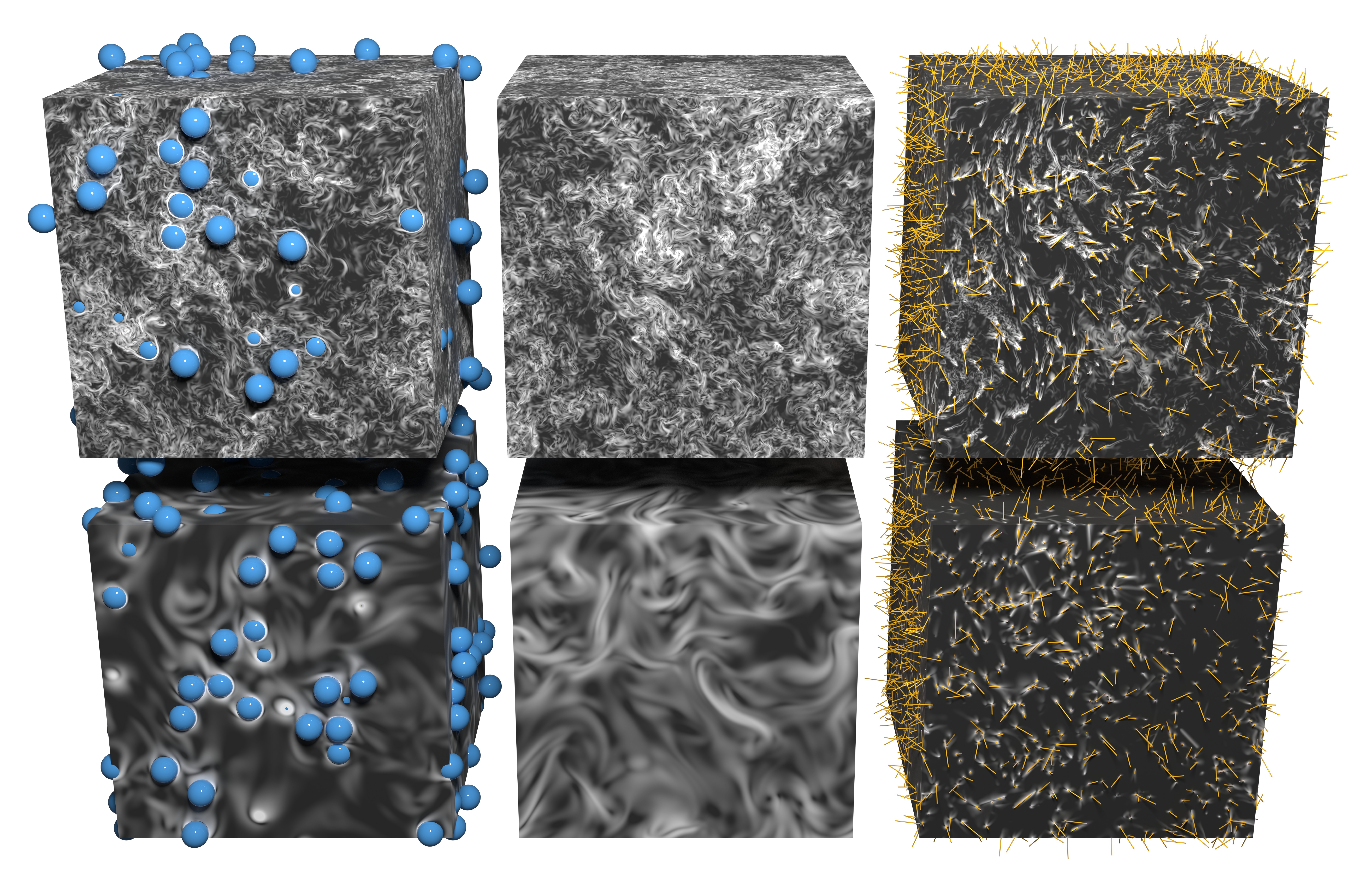
Figure 1: Images of the simulated domain. Left column: flows with fixed spheres. Middle column: single phase flows. Right column: flows with fixed fibres. Flows on the top row have $Re_{ABC}=894$. Flows on the bottom row have $Re_{ABC}=55.9$. At the boundary of each domain we show the dissipation on a logarithmic scale, where $\epsilon_{s}$ is the mean dissipation of the single-phase flow at $Re_{ABC}=894$.

I Introduction

Particle-laden turbulent flows abound in our environment; see, for example, volcanic ash clouds, sandstorms, and microplastics in the oceans. In these cases, the particles are seen in a range of shapes, and the intensity of the carrier turbulent flow can significantly vary. In this context, the present study delves into the interaction between particles and turbulent flows, focusing on two distinct particle shapes, spheres and fibres, and exploring turbulent flows across a large range of Reynolds numbers.

The interaction of particles with turbulent flows has garnered significant research attention since Richardson and Proctor [1] used balloons to track eddies in the Earth’s atmosphere in 1927. Light spherical particles as tracers are now a ubiquitous experimental tool [2], and even fibre-shaped tracers have been employed [3]. For heavier particles, more complex motion is seen, such as inertial clustering [4] and preferential sampling [5]. Numerical simulations in this field have been a valuable tool, as results can be readily processed to study length-scale dependent statistics such as radial distribution functions [6], and histograms of Voronoï area [4]. Most of such particle-laden turbulent studies make the one-way coupling assumption, whereby the particles are affected by the fluid motion, but the fluid does not feel any effect of the particles. When the total mass fraction or volume fraction of particles in the system increases, the one-way coupling assumption becomes invalid, and we must model the back-reaction effect of the particles on the fluid. This opens up a zoo of new phenomena, including drag reduction [7], cluster-induced turbulence [8], and new scalings in the energy spectrum [9]. A recent review by Brandt and Coletti [10] has pointed out a gap in the current understanding of particles in turbulence, which lies between small heavy particles and large weakly buoyant particles. In addition, most real-world particle-laden flows involve particles with a high degree of anisotropy, while research in particle-laden turbulence has overwhelmingly focused on spherical particles.

This article addresses the gaps by studying a range of particle mass fractions $M$, ranging from single-phase ($M=0$) to fixed particles ($M=1$). We make simulations using a fully coupled approach to elucidate how particles modulate turbulence. Furthermore, we vary the turbulence intensity, allowing us to ask the question at what Reynolds numbers ($Re$) does turbulence modulation emerge? And does the modulation effect persist as $Re\to\infty$? Crucially, we connect our results to real-world flows by investigating isotropically-shaped particles (spheres) and anisotropically-shaped particles (fibres). The spheres have a single characteristic length, given by their diameter, whereas the fibres have two: their length and thickness. This naturally allows us to ask how do the particle’s characteristic lengths impact the scales of the turbulent flow?

A number of works have investigated particle shape, see Voth and Soldati [18] for a review of the behaviour of anisotropic particles in turbulence, including oblate spheroids, prolate spheroids and fibres. In 1932 Wadell [11] defined the sphericity of a particle as its surface area divided by the area of a sphere with equivalent volume; Wadell used the sphericity to classify quartz rocks according to their shape. More recently, Zhao et al. [14] made direct numerical simulations of oblate and prolate spheroids in a channel flow, and found that away from the channel walls, prolate spheroids tend to rotate about their symmetry axis (spinning), whereas oblate particles rotate about an axis perpendicular to their symmetry axis (tumbling). Ardekani et al. [17] showed that oblate spheroids can reduce drag in a turbulent channel by aligning their major axes parallel to the wall. Yousefi et al. [16] simulated spheres and oblate spheroids in a shear flow, and found that the rotation of the spheroids can enhance the kinetic energy of the flow. At the other shape extreme from oblate spheroids, we have fibres, which are long and thin. In this article, we choose to study rigid fibres (also known as rods) as they are a simple example of a particle with high anisotropy. Concerning fibres, Paschkewitz et al. [12], Gillissen et al. [13] and others showed that rigid fibres align with vorticity in channel flows, dissipating the vortex structures, and drag reductions up to 26% have been measured [12]. In this article, we wish to investigate how the shapes and length scales of particles interact with turbulence, so we choose the triperiodic flow geometry. This geometry avoids the effects of walls and other large structures on the flow, enabling us to focus on the emergent length scales of the flow.

A few works have investigated the effect of turbulence intensity on particle-laden flows. Lucci et al. [19] simulated spheres of various diameters $c$ in decaying isotropic turbulence, and found that spheres reduce the fluid kinetic energy and enhance dissipation when $c>\eta$, where $\eta$ is the Kolmogorov length scale. In this article, we also vary the ratio $c/\eta$, however, unlike [19], we do it by varying the fluid viscosity, not the particle size. This enables us to keep the particle volume, particle surface area and number of particles constant across our cases. Oka and Goto [20] studied sphere diameters in the range $7.8<c/\eta<64$, in turbulent flows with $Re_{\lambda}\approx 94$ and showed that vortex shedding and turbulence attenuation occur when $c\gtrsim\lambda\rho/\tilde{\rho}$, where $\lambda$ is the Taylor length-scale, $\rho$ and $\tilde{\rho}$ are the fluid and solid densities, respectively. Shen et al. [22] investigated the effect of solid-fluid density ratio for flows with $38<Re_{\lambda}<74$, and $8.8<c/\eta<18$, showing that higher density spheres cause more turbulence attenuation. Peng et al. [21] parametrized the attenuation of turbulent kinetic energy by spheres with $7.1<c/\eta<15$ and $41<Re_{\lambda}<63$. They found that the particle mass fraction is indeed a strong indicator of attenuation and that there is negligible dependence on the Taylor Reynolds number $Re_{\lambda}$ for this range. Compared to the above works, we choose a wider range of turbulence intensities, such that $11.7<c/\eta<125$ and $12.8<Re_{\lambda}<442$, and we extend the study to include non-spherical particles.

This article is structured as follows: In the following section, we describe the numerical methods and the parameters used in our study. In section III, we present and discuss the results of our simulations, and section IV concludes with a summary and outlook on future research.

II Methods and setup

We tackle the problem using large direct numerical simulations on an Eulerian grid of $1024^{3}$ points with periodic boundaries in all three directions. To obtain the fluid velocity $u_{i}$ and pressure $p$, we solve the incompressible Navier-Stokes equations for a Newtonian fluid with kinematic viscosity $\nu$ and density $\rho$,

$$\partial_{t}u_{i}+\partial_{j}(u_{i}u_{j}) =\nu\partial_{jj}u_{i}-\partial_{i}p/\rho+f^{ABC}_{i}+f^{sf}_{i},$$ (1)

$$\partial_{j}u_{j} =0,$$ (2)

where indices $i,j\in\{1,2,3\}$ denote the Cartesian components of a vector, and repeated indices are implicitly summed over. The turbulent flow is sustained by an ABC forcing [23, 24], which is made of sinusoids with a wavelength $2\pi L$ equal to the domain size,

$$\begin{split}f^{ABC}_{1}=F\sin({x_{3}}/{L})+F\cos({x_{2}}/{L}),\\ f^{ABC}_{2}=F\sin({x_{1}}/{L})+F\cos({x_{3}}/{L}),\\ f^{ABC}_{3}=F\sin({x_{2}}/{L})+F\cos({x_{1}}/{L}).\end{split}$$ (3)

The amplitude $F$ of the forcing is used to define the forcing Reynolds number ${Re_{ABC}\equiv F^{1/2}L^{3/2}/\nu}$. To discern the effect of increasing turbulence intensity, we conduct a number of simulations with various values of $Re_{ABC}$, given in table 1.

When the single-phase flows reach a statistically steady state, we add the solid particles at random (non-overlapping) locations in the domain. We allow the flow to reach a statistically steady state again, and measure the statistics presented in section III, which were averaged in time over multiple large-eddy turnover times $\tau_{f}\equiv 2\pi L/u^{\prime}$, where $u^{\prime}$ is the root mean square of the fluid velocity. This procedure is repeated for every solid mass fraction investigated, defined as $M\equiv m_{s}/(m_{s}+m_{f})$ where $m_{s}$ and $m_{f}$ are the total mass of solid and fluid. The single-phase cases have $M=0$, and the cases with fixed particles have $M=1$. The solid phase is two-way coupled to the fluid using the immersed boundary method, and the back-reaction of the particles on the fluid is enforced by $\mathbf{f^{sf}}$ in equation 1. As can be seen in figure 1, we simulate two types of particles, spheres and fibres; to isolate the effect of particle isotropy on the flow, we choose the fibres and spheres to have the same size: the spheres have diameter $c$, and the fibres have length $c$, where ${c=L/2}$ in all cases.

We use the in-house Fortran code Fujin to solve the flow numerically. Time integration is carried out using the second-order Adams-Bashforth method, and incompressibility (equation 2) is enforced in a pressure correction step [25], which uses the fast Fourier transform. Variables are defined on a staggered grid; velocities and forces are defined at the cell faces, while pressure is defined at the cell centres. Second-order finite differences are used for all spatial gradients. See https://groups.oist.jp/cffu/code for validations of the code.

II.1 Motion of the spheres

The sphere motion and forces are modelled using an Eulerian-based immersed boundary method developed by Hori et al. [26]. The velocity $\mathbf{U}$ and rotation rate $\mathbf{\Omega}$ of each sphere are found by integrating the Newton-Euler equations in time

$$m\partial_{t}U_{i} =\oiint_{S}\left(\rho\nu(\partial_{i}u_{j}+\partial_{j}u_{i})-p\delta_{ij}\right)n_{j}dS-F^{col}n_{i},$$ (4)

$$I\partial_{t}\Omega_{i} =\oiint_{S}\epsilon_{ijk}\frac{c}{2}n_{j}\rho\nu(\partial_{k}u_{l}+\partial_{l}u_{k})n_{l}dS,$$ (5)

where $\delta_{ij}$ is the Kronecker delta and $\epsilon_{ijk}$ is the Levi-Civita symbol, $S$ is the surface of the sphere, and $\mathbf{n}$ is its normal. ${m=\tilde{\rho}\pi c^{3}/6}$ and ${I=mc^{3}/20}$ are the mass and moment of inertia of the sphere with diameter $c$ and density $\tilde{\rho}$. A soft-sphere collision force $F^{col}\mathbf{n}$ is applied in the radial direction when spheres overlap [26].

Table 2 shows our choice of parameters for the sphere-laden flows. In all cases, we use 300 spheres. The characteristic time of the spheres is $\tau_{s}=\tilde{\rho}c^{2}/(18\rho\nu)$, from which we can define the Stokes number $St\equiv\tau_{s}/\tau_{f}$ of our flows. The particle Reynolds number is $Re_{p}=c\sqrt{\langle\mathbf{\Delta u}_{n}\cdot\mathbf{\Delta u}_{n}\rangle_{n}}/\nu$, where $\mathbf{\Delta u}_{n}$ is the difference between the velocity of the $n$th particle and the local fluid velocity, averaged in a ball of diameter $2c$ centred on the sphere. The angled brackets $\langle\rangle_{n}$ denote an average over all spheres in the simulation.

II.2 Motion of the fibres

For the motion and coupling of the fibres, we also use an immersed boundary method, but this one is Lagrangian and solves the Euler-Bernoulli equation for the position $\mathbf{X}$ of the beam with coordinate $l$ along its length [27, 28, 29]

$$\frac{\pi}{4}d^{2}(\tilde{\rho}-\rho)\partial^{2}_{t}X_{i}=\partial_{l}(T\partial_{l}X_{i})+\gamma\partial^{4}_{l}X_{i}-F^{fs}_{i}+F^{col}_{i},$$ (6)

where $T$ is the tension, enforcing the inextensibility condition;

$$\partial_{t}X_{i}\partial_{t}X_{i}=1.$$ (7)

The volumetric density of the fibre is $\tilde{\rho}$, and its stiffness is $\gamma$. Note that, the fluid density $\rho$ in equation 6 cancels the inertia of the fluid in the fictitious domain inside the fibre [30]. To exclude deformation effects in our study, we choose a stiffness which limits the fibre deformation below 1%. The collision force $\mathbf{F^{col}}$ is the minimal collision model by Snook et al. [31]. The fluid-solid coupling force $\mathbf{F^{fs}}$ enacts the non-slip condition at the particle surface, and an equal and opposite force ($\mathbf{f^{sf}}$ in equation 1) acts on the fluid. The spreading kernel onto the Eulerian grid has a width of three grid spaces, giving the fibre diameter $d=3\Delta x$ in units of the Eulerian grid spacing. Table 3 shows our choice of parameters for the fibre-laden flows, where we use $10^{4}$ fibres in all cases. The characteristic time of the fibres is calculated using a formulation which takes their aspect ratio $\beta\equiv c/d$ into account [32],

$$\tau_{s}=\frac{\tilde{\rho}d^{2}}{18\rho\nu}\frac{\beta\ln\left(\beta+\sqrt{\beta^{2}-1}\right)}{\sqrt{\beta^{2}-1}},$$ (8)

from which we can define the Stokes number $St\equiv\tau_{s}/\tau_{f}$ of our flows. The particle Reynolds number of the fibres is $Re_{p}=d\sqrt{\langle\mathbf{\Delta u}_{n}\cdot\mathbf{\Delta u}_{n}\rangle_{n}}/\nu$, where $\mathbf{\Delta u}_{n}$ is the difference between the velocity of the midpoint of the $n$th fibre and the local fluid velocity, averaged in a ball of diameter $2c$ centred on the fibre’s midpoint. The angled brackets $\langle\rangle_{n}$ denote an average over all fibres in the simulation.

marker	$Re_{ABC}$	$M$	$\eta/L$	$Re_{\lambda}$	$\epsilon\mathcal{L}/u^{\prime 3}$
$\pentagonblack$	$\mathbf{894}$	0.0	${4.06\times 10^{-3}}$	433	0.399
$\blacksquare$	$447$	0.0	$6.31\times 10^{-3}$	308	0.382
$\blacktriangle$	$224$	0.0	$1.11\times 10^{-2}$	204	0.400
$\blacklozenge$	$112$	0.0	$1.95\times 10^{-2}$	116	0.473
$\mdlgblkcircle$	$\mathbf{55.9}$	0.0	${2.99\times 10^{-2}}$	101	0.428

Table 1: Single-phase flows. $Re_{ABC}$ is the forcing Reynolds number, and $M$ is the solid mass fraction. We measure the Kolmogorov length scale $\eta\equiv\nu^{3/4}/\epsilon^{1/4}$, the Taylor Reynolds number $Re_{\lambda}$, and the dissipation $\epsilon$, which has been normalised using the integral length scale $\mathcal{L}$ and the root mean square velocity $u^{\prime}$ of the fluid. The largest and smallest values of each parameter are shown in bold.

marker	$Re_{ABC}$	$M$	$\tilde{\rho}/\rho$	$\eta/L$	$Re_{\lambda}$	$\epsilon\mathcal{L}/u^{\prime 3}$	$St$	$Re_{p}$
$\pentagonblack$	$\mathbf{894}$	0.1	1.29	$4.09\times 10^{-3}$	431	0.397	7.4	618
$\pentagonblack$	$\mathbf{894}$	0.3	4.99	$4.18\times 10^{-3}$	397	0.395	26.9	857
$\pentagonblack$	$\mathbf{894}$	0.6	17.4	$4.09\times 10^{-3}$	346	0.507	89.1	$1.12\times 10^{3}$
$\pentagonblack$	$\mathbf{894}$	0.9	105	$4.18\times 10^{-3}$	280	0.625	471	$1.18\times 10^{3}$
$\pentagonblack$	$\mathbf{894}$	1.0	$\boldsymbol{\infty}$	$4.29\times 10^{-3}$	247	0.708	$\boldsymbol{\infty}$	$\mathbf{1.19\times 10^{3}}$
$\blacksquare$	$447$	1.0	$\boldsymbol{\infty}$	$7.31\times 10^{-3}$	161	0.786	$\boldsymbol{\infty}$	559
$\blacktriangle$	$224$	0.1	1.29	$1.13\times 10^{-2}$	219	0.374	1.91	142
$\blacktriangle$	$224$	0.3	4.99	$1.16\times 10^{-2}$	181	0.477	6.49	198
$\blacktriangle$	$224$	0.6	17.4	$1.18\times 10^{-2}$	157	0.586	20.9	243
$\blacktriangle$	$224$	0.9	105	$1.19\times 10^{-2}$	123	0.751	109	266
$\blacktriangle$	$224$	1.0	$\boldsymbol{\infty}$	$1.26\times 10^{-2}$	101	0.936	$\boldsymbol{\infty}$	260
$\blacklozenge$	$112$	1.0	$\boldsymbol{\infty}$	$2.14\times 10^{-2}$	61.5	1.19	$\boldsymbol{\infty}$	117
$\mdlgblkcircle$	$\mathbf{55.9}$	1.0	$\boldsymbol{\infty}$	$3.60\times 10^{-2}$	34.9	1.81	$\boldsymbol{\infty}$	44.6

Table 2: Sphere-laden flows. We set the solid-fluid density ratio $\tilde{\rho}/\rho$ to obtain a range of solid mass fractions $M$. Bulk statistics for the particles are the Stokes number $St$ and the particle Reynolds number $Re_{p}$. The largest and smallest values of each parameter are shown in bold.

marker	$Re_{ABC}$	$M$	$\tilde{\rho}/\rho$	$\eta/L$	$Re_{\lambda}$	$\epsilon\mathcal{L}/u^{\prime 3}$	$St$	$Re_{p}$
$\pentagonblack$	$\mathbf{894}$	0.2	47.2	$4.09\times 10^{-3}$	422	0.425	1.45	34.9
$\pentagonblack$	$\mathbf{894}$	0.3	81.8	$\mathbf{4.02\times 10^{-3}}$	442	0.432	2.6	41.2
$\pentagonblack$	$\mathbf{894}$	0.6	279	$4.17\times 10^{-3}$	340	0.713	7.52	46.4
$\pentagonblack$	$\mathbf{894}$	0.9	$1.69\times 10^{3}$	$4.26\times 10^{-3}$	223	1.15	36.1	47.2
$\pentagonblack$	$\mathbf{894}$	1.0	$\boldsymbol{\infty}$	$4.40\times 10^{-3}$	201	1.29	$\boldsymbol{\infty}$	46.0
$\blacksquare$	$447$	1.0	$\boldsymbol{\infty}$	$7.44\times 10^{-3}$	115	1.78	$\boldsymbol{\infty}$	20.6
$\blacktriangle$	$224$	0.1	21.3	$1.16\times 10^{-2}$	192	0.434	0.155	8.31
$\blacktriangle$	$224$	0.3	81.8	$1.16\times 10^{-2}$	196	0.465	0.605	9.9
$\blacktriangle$	$224$	0.6	279	$1.19\times 10^{-2}$	167	0.63	1.85	11.2
$\blacktriangle$	$224$	0.9	$1.69\times 10^{3}$	$1.23\times 10^{-2}$	72.5	2.25	7.16	9.11
$\blacktriangle$	$224$	1.0	$\boldsymbol{\infty}$	$1.29\times 10^{-2}$	54.9	3.17	$\boldsymbol{\infty}$	8.22
$\blacklozenge$	$112$	1.0	$\boldsymbol{\infty}$	$2.33\times 10^{-2}$	28.8	4.68	$\boldsymbol{\infty}$	3.32
$\mdlgblkcircle$	$\mathbf{55.9}$	1.0	$\boldsymbol{\infty}$	$\mathbf{4.27\times 10^{-2}}$	12.8	8.60	$\boldsymbol{\infty}$	1.51

Table 3: Fibre-laden flows. We set the solid-fluid density ratio $\tilde{\rho}/\rho$ to obtain a range of solid mass fractions $M$. Bulk statistics for the particles are the Stokes number and particle Reynolds number. The largest and smallest values of each parameter are shown in bold.

III Results and discussion

III.1 Bulk statistics

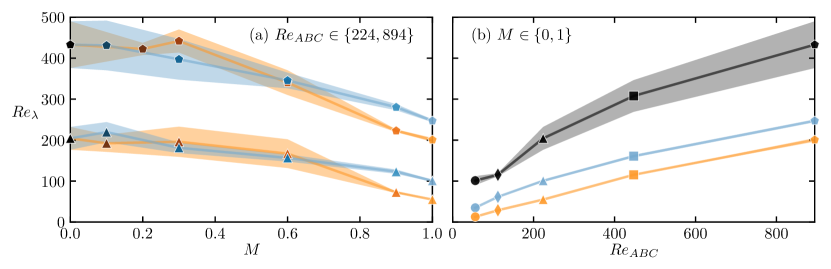
Figure 2: (a) Effect of the solid mass fraction $M$ on the Taylor Reynolds number $Re_{\lambda}$. Flows with $Re_{ABC}=224$ are marked using triangles, and flows with $Re_{ABC}=894$ are marked using pentagons. (b) Effect of the forcing Reynolds number $Re_{ABC}$ on the Taylor Reynolds number $Re_{\lambda}$, for the single phase and particle-laden cases with fixed particles ($M=1$). In both plots, we show the single-phase flows in black, flows with spheres in blue, and flows with fibres in yellow; the shaded regions give the root-mean-square of $Re_{\lambda}$ in time.

The Taylor Reynolds number is defined as $Re_{\lambda}\equiv u^{\prime}\lambda/\nu$, where $u^{\prime}$ is the root-mean-square velocity averaged over space and time, $\lambda=u^{\prime}\sqrt{15\nu/\epsilon}$ is the Taylor length scale, and $\epsilon$ is the viscous dissipation rate averaged over space and time. The Taylor-Reynolds number is an indicator of the intensity of turbulence in the flow, and in figure 2, we show how $Re_{\lambda}$ compares for all of our cases. Figure 2a shows that increasing the solid mass fraction $M$ causes a reduction in $Re_{\lambda}$ at both high and low forcing Reynolds numbers. Both spheres and fibres produce a comparable decrease in $Re_{\lambda}$, but the reduction effect is more substantial for very heavy fibres. Looking at the trend in $Re_{\lambda}$ with the forcing Reynolds number $Re_{ABC}$ in figure 2b, we see, as expected, a monotonic increase in all three cases, i.e., single phase, sphere-laden, and fibre-laden flows.

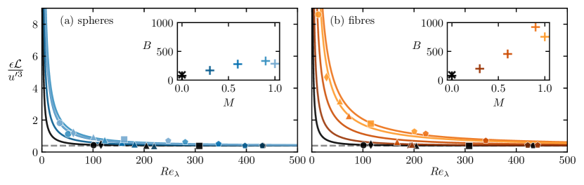
Figure 3: The dependence of the normalised dissipation $\epsilon\mathcal{L}/u^{\prime 3}$ on the Taylor-Reynolds number $Re_{\lambda}$. Flows with spheres are marked blue on panel (a), flows with fibres are marked in orange on panel (b), and single-phase flows are marked in black on both panels. Dashed lines show the anomalous value of dissipation $\epsilon\mathcal{L}/u^{\prime 3}=0.4$ measured by Donzis et al. [33]. Solid lines show fits of equation 10 with $A=0.2$. The fitted values of $B$ are given in the inset, where Donzis’ result $(B=92)$ is marked with an ‘X’.

The dissipative anomaly is a well-studied feature in single-phase turbulent flows, first proposed by Taylor [34]. It states that the normalised dissipation $\epsilon\mathcal{L}/u^{\prime 3}$ remains finite, even in the limit of vanishing viscosity ($Re_{\lambda}\to\infty$), where we calculate the integral length scale $\mathcal{L}$ from the energy spectrum

$$\mathcal{L}=\frac{\pi}{2u^{\prime 2}}\int_{0}^{\infty}\frac{E}{\kappa}\mathrm{d}\kappa.$$ (9)

Donzis et al. [33] parametrized the dissipative anomaly, based on the analysis of Doering and Foias [35], and they fit the function

$$\frac{\epsilon\mathcal{L}}{u^{\prime 3}}=A\left[1+\sqrt{1+(B/Re_{\lambda})^{2}}\right]$$ (10)

to a number of single-phase flows, obtaining $A=0.2$ and $B=92$. Figure 3 shows the dependence of the normalised dissipation for our flows. We see that as $Re_{\lambda}\to\infty$, flows with spheres and fibres at all mass fractions appear to converge to the same anomalous value of dissipation $\epsilon\mathcal{L}/u^{\prime 3}=0.4$. Hence, we fit equation 10 with $A=0.2$ to each mass fraction of spheres and fibres, obtaining a value for $B$ in each case, shown in the insets of figure 3. The fit to our single phase flows agrees closely with Donzis et al. [33]’s result. However, both spheres and fibres cause an increase in the value of $B$ as their mass fraction increases, with fibres producing roughly double the effect. To understand how spheres and fibres modify the dissipation in the flow, we must look at how they transport energy from large to small scales, into the dissipative range.

III.2 Scale-by-scale results

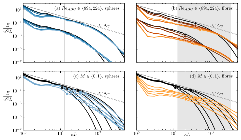
Figure 4: Energy spectra of all cases. On the left, we show flows with spheres, and the vertical grey lines show the wavenumber $\kappa_{c}=2\pi/c$ of the sphere diameter. On the right, we show flows with fibres, and we shade the region between the wavenumber $\kappa_{c}$ of the fibre length and the wavenumber $\kappa_{d}=2\pi/d$ of the fibre diameter. (a) and (b) show $Re_{ABC}=894$ and $Re_{ABC}=224$, with the latter shifted downwards by a factor of 100 on the y-axis, for various mass fractions. (c) and (d) show fixed $(M=1)$ and single phase $(M=0)$ cases for various Reynolds numbers. Markers are at the wavenumber corresponding to the Taylor length scale.

Figure 4 shows each flow’s turbulent kinetic energy spectrum $E$. Single-phase flows exhibit the canonical Kolmogorov scaling $E\sim\kappa^{-5/3}$ for one or two decades, depending on the forcing Reynolds number. Adding spheres reduces $E$ at wavenumbers up to the sphere diameter ($\kappa<\kappa_{c}$) and increases $E$ in the dissipative range. We mention, in passing, the oscillations at the wavenumber of the sphere diameter; these are an artefact resulting from the discontinuity in the velocity gradient at the sphere boundary [19]. The addition of fibres causes a reduction in $E$ across a broad band of wavelengths ($\kappa L\lesssim 100$) and a pronounced increase in the dissipative range. As was previously seen by Olivieri et al. [9], the energy scaling $E\sim\kappa^{-\beta}$ becomes flatter as the mass fraction $M$ of fibres increases. Figure 4 also shows that both spheres and fibres cause the Taylor length scale to shift to higher wavenumbers due to the increase of the energy in the dissipative scales due to the presence of particles.

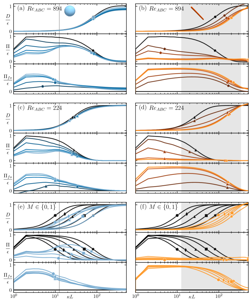
Figure 5: Scale-by-scale energy balance for all cases. Panels (a) and (b) show $Re_{ABC}=894$ cases for various mass fractions. Panels (c) and (d) show $Re_{ABC}=224$ cases for various mass fractions. Panels (e) and (f) show fixed ($M=1$) and single-phase ($M=0$) cases for various Reynolds numbers. On the left, we show flows with spheres, and the vertical grey lines show the wavenumber $\kappa_{c}=2\pi/c$ of the sphere diameter. On the right, we show flows with fibres, and we shade the region between the wavenumber $\kappa_{c}$ of the fibre length and the wavenumber $\kappa_{d}$ of the fibre diameter. For each case, we plot three terms: the Dissipation $D$, the energy flux $\Pi$ due to convection, and the energy flux $\Pi_{fs}$ due to the fluid-solid coupling. Each curve is marked where the gradient is largest.

Figure 5 shows how each term in the Navier-Stokes equation interacts with the energy spectrum; this is expressed by the spectral energy balance ${\mathcal{F}_{inj}(\kappa)+\Pi(\kappa)+\Pi_{fs}(\kappa)+{D}(\kappa)=\epsilon}$, where $\mathcal{F}_{inj},\Pi,\Pi_{fs},$ and $D$ are the rate of energy transfer by the ABC forcing, advection, fluid-solid coupling, and dissipation, respectively. See the supplementary information of Ref. [36] for a derivation of this equation. For the single-phase flows, energy is carried by the advective term $\Pi$ from large to small scales, where it is dissipated by the viscous term $D$. When particles are added, we see that the fluid-solid coupling term $\Pi_{fs}$ acts as a ‘spectral shortcut’ [37, 9]; it bypasses the classical turbulent cascade, removing energy from large scales and injecting it at the length scale of the particle trough their wake. In keeping with the spectra, the power of the fluid-solid coupling (shown by the peak value of $\Pi_{fs}$) increases with mass fraction $M$ of both spheres and fibres. For spheres, the coupling $\Pi_{fs}$ dominates only at wavenumbers less than that of the sphere diameter $\kappa<\kappa_{c}$ (i.e., large length scales). Around $\kappa_{c}$, the sphere wake returns energy to the fluid, and the classical cascade resumes for $\kappa>\kappa_{c}$. For fibres instead, $\Pi_{fs}$ extends deep into the viscous range: in fact, markers on the $\Pi_{fs}$ curves show that spheres mostly inject energy around the length scale of their diameter , and fibres mostly inject energy at a length scale between their thickness and length. This observation is supported by the images of dissipation in figure 1; around the spheres, we see wakes comparable in size to their diameter, while around the fibres, we see wakes comparable in size to their thickness. We presume that the fluid-sphere coupling $\Pi_{fs}$ would also extend into the viscous range if the sphere diameter was in this range. Lastly, we consider the effect of Reynolds number on energy transfers in the flow, reducing $Re_{ABC}$ limits the range of scales at which the advective flux $\Pi$ occurs for single-phase flows. However, $Re_{ABC}$ has little effect on the wavenumber range of the fluid-solid coupling term $\Pi_{fs}$, suggesting that the size of the particle wakes is governed mainly by particle geometry, with a lesser effect from fluid properties like viscosity.

Figure 6: Structure functions of order $p=2$ (dashed lines) and $p=6$ (solid lines). Panels (a) and (b) show cases with $Re_{ABC}=894$ for various mass fractions. Panels (c) and (d) show cases with $Re_{ABC}=224$ for various mass fractions. Panels (e) and (f) show fixed ($M=1$) and single-phase ($M=0$) cases for various Reynolds numbers. Flows with spheres are on the left, and flows with fibres are on the right. Grey lines show the scalings predicted by Kolmogorov for the single-phase structure functions. We mark each line at $r=c$.

Moving from wavenumber space to physical space, we show the longitudinal structure functions $S_{p}\equiv\langle\left[\hat{r}_{i}u_{i}(\mathbf{x}+\mathbf{r})-\hat{r}_{i}u_{i}(\mathbf{x})\right]^{p}\rangle$ of each flow in figure 6, where $\mathbf{r}$ is a separation vector between two points in the flow, it has magnitude $r$ and direction $\mathbf{\hat{r}}$, and angled brackets show an average over space $\mathbf{x}$. For the second moment $(p=2)$, the single-phase flows closely follow Kolmogorov’s scaling in the inertial range ($r\gg\eta$). However, when particles are added, $S_{2}$ decreases relative to the single-phase case. For spheres, the decrease occurs for $r\gtrsim c$, while for fibres, it occurs at even smaller separations $r$. Much like the $E\sim k^{-\beta}$ scalings seen in figure 4, the decreased regions in figure 6 show scalings $S_{2}\sim r^{\zeta_{2}}$, which become flatter for larger mass fractions $M$. These energy spectrum and structure-function scalings are, in fact, just observations of the same phenomenon, as the exponents are related by $\zeta_{2}=\beta-1$ for any differentiable velocity field [38, p.232]. In the higher moment structure function ($p=6$), the flattening of the $S_{6}\sim r^{\zeta_{6}}$ scaling by the particles is yet more apparent, indicating that the tails of the probability distribution of $\hat{r}_{i}u_{i}(\mathbf{x}+\mathbf{r})-\hat{r}_{i}u_{i}(\mathbf{x})$ become wider for smaller separations $r$. In other words, extreme values become more common, and the velocity field becomes more intermittent in space. In the case of single-phase homogeneous-isotropic turbulence, the intermittency of the velocity field has been attributed to the non-space-filling nature of the fluid dissipation [39]. Next, we explore this link in the case of particle-laden turbulence by investigating the intermittency of dissipation $\epsilon$ in space.

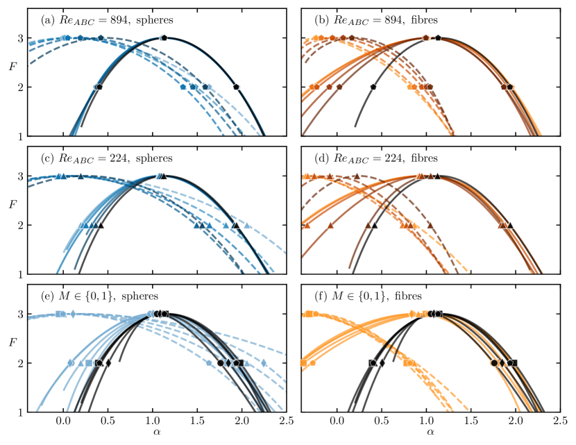
Figure 7: Multifractal spectra of the dissipation in regions containing particles (dashed lines) and regions not containing particles (solid lines). Panels (a) and (b) show cases with $Re_{ABC}=894$ for various mass fractions. Panels (c) and (d) show cases with $Re_{ABC}=224$ for various mass fractions. Panels (e) and (f) show fixed ($M=1$) and single-phase ($M=0$) cases for various Reynolds numbers. Flows with spheres are on the left, and flows with fibres are on the right. We mark each line where $F$ is maximum and at $F=2$.

Using the method described by Frisch [39, p.159], we obtain the quantity $\epsilon_{l}$ by averaging the dissipation within a ball of radius $6\Delta x\leq l\leq 10\Delta x$ and take a moment $-6\leq q\leq 6$ of this quantity; if the dissipation field is multifractal, the ensemble average has a scaling behaviour $\langle\epsilon_{l}^{q}\rangle\sim l^{\tau_{q}}$ and we can obtain the multifractal spectrum $F$ with an inverse Legendre transformation,

$$\tau_{q}=\min_{\alpha}[q(\alpha-1)+3-F],$$ (11)

where $\min_{\alpha}$ states that we take the value of $\alpha$ which minimizes the expression in the square brackets. Figure 7 shows the multifractal spectra for all cases. Similarly to Mukherjee et al. [40], we split our analysis into separate regions: solid curves result from an ensemble average over balls not containing particles, while dashed curves result from an ensemble average over balls containing particles, where the radius $l$ has been rescaled according to the volume $V_{f}$ of fluid remaining in the ball, i.e., $l=(3V_{f}/4\pi)^{1/3}$. We see that the multifractal spectra of the single-phase flows and the regions not containing particles have peaks at $\alpha\approx 1,F\approx 3$, showing there is a background of space-filling dissipation in these regions [39, p.163].

The multifractal spectra of the regions containing spheres (blue dashed lines in figure 7) have peaks which are shifted to the left. This shift can be explained by considering the high dissipation in the boundary layers around the spheres. As imaged in figure 1, the boundary layers are confined in space to relatively thin sheets. The volume of a thin sheet intersecting with a ball of radius $l$ is $V\sim l^{2}$, hence the total dissipation in a ball intersecting with a spherical particle also scales as $\sim l^{2}$. When we average over the volume of the ball ($\sim l^{3}$) and take the $q$th moment, we obtain $\langle\epsilon_{l}^{q}\rangle\sim l^{2q}l^{-3q}$, and this scales as $\tau_{q}=-q$. By equation 11, this is the Legendre transformation of the point $\alpha=0,F=3$, which is roughly where the peaks in the multifractal spectra are located.

The multifractal spectra of the regions containing fibres (orange dashed lines in figure 7) have peaks which are shifted even further to the left. Again, we explain this by considering the wakes around the particles. Suppose that the dissipation around a fibre is confined to a thin tube. In this case, the volume of a tube intersecting with a ball of radius $l$ is $V\sim l$, thus in this case $\langle\epsilon_{l}^{q}\rangle\sim l^{q}l^{-3q}$, so the resulting scaling is $\tau_{q}=-2q$, which (by equation 11) is the Legendre transformation of the point $\alpha=-1,F=3$. In fact, from the bottom right panel of figure 7, we see that the ensemble average over balls containing $M=1$ fibres produces peaks in the region $-0.5<\alpha<0$, suggesting that the wakes around the fibres are not exactly thin tubes, but more space-filling structures with a dimension greater than one. This is also supported by the images in figure 1, as the wakes are seen to extend behind the fibres.

The middle and upper panels of figure 7 show that (at $Re_{ABC}=224$ and $Re_{ABC}=894$) the sphere- and fibre-containing multifractal spectra tend toward the single phase multifractal spectrum as $M$ is reduced. This is expected, as the particle-fluid relative velocity is reduced and the wakes become less prominent compared to the background space-filling turbulence. On the other hand, the ensembles of balls not containing particles produce multifractal spectra with low $\alpha$ tails that extend beyond those of the single-phase multifractal spectra, suggesting that the wakes of spheres and fibres extend into the bulk of the fluid and that they retain their non-space-filling nature.

III.3 Local flow structures

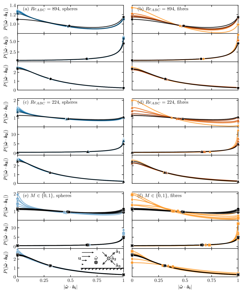
Figure 8: Histograms of the alignment of the vorticity unit vector $\boldsymbol{\hat{\omega}}$ with the eigenvectors $\mathbf{\hat{a}_{1}},\mathbf{\hat{a}_{2}},\mathbf{\hat{a}_{3}}$ of the strain-rate tensor. Flows with spheres are on the left, and flows with fibres are on the right. Panels (a) and (b) show cases with $Re_{ABC}=894$ for various mass fractions. Panels (c) and (d) show cases with $Re_{ABC}=224$ for various mass fractions. Panels (e) and (f) show fixed ($M=1$) and single-phase ($M=0$) cases for various Reynolds numbers. We mark each line at $|\boldsymbol{\hat{\omega}}\cdot\mathbf{\hat{a}_{i}}|=0,1$ and $\langle|\boldsymbol{\hat{\omega}}\cdot\mathbf{\hat{a}_{i}}|\rangle$. The inset of panel (e) shows the directions of vorticity and the eigenvectors of the strain rate in a laminar shear flow above a flat non-slip surface, where $\mathbf{\hat{a}_{1}}$ and $\mathbf{\hat{a}_{3}}$ are confined to the shear plane, while $\mathbf{\hat{a}_{2}}$ and $\boldsymbol{\hat{\omega}}$ are perpendicular to it.

To look more closely at the flow structures produced by the particles, we compute the alignment of the unit-length eigenvectors $\mathbf{\hat{a}_{1},\hat{a}_{2},\hat{a}_{3}}$ of the strain-rate tensor ${s_{ij}\equiv(\partial_{i}u_{j}+\partial_{j}u_{i})/2}$ with the vorticity ${\boldsymbol{\omega}\equiv\epsilon_{ijk}\partial_{j}u_{k}\mathbf{\hat{e}}_{i}}$ [41, 42], where $\mathbf{\hat{e}_{1},\hat{e}_{2},\hat{e}_{3}}$ are the Cartesian unit vectors. We choose $\mathbf{\hat{a}_{1}}$ to be the eigenvector corresponding to the largest eigenvalue. For an incompressible fluid, the three eigenvalues of $s_{ij}$ sum to zero, so the largest eigenvalue is never negative. Hence, $\mathbf{\hat{a}_{1}}$ aligns with the direction of elongation in the flow. Similarly, we choose the eigenvector $\mathbf{\hat{a}_{3}}$ to correspond with the smallest eigenvalue, which is never positive, so $\mathbf{\hat{a}_{3}}$ aligns with the direction of compression in the flow. Finally, due to the symmetry of the strain-rate tensor, $\mathbf{\hat{a}_{2}}$ is orthogonal to the other two eigenvectors and, depending on the flow, there can be compression or elongation along its axis. Figure 8 shows probability-density functions $P$ of the scalar product of the unit-length vorticity $\boldsymbol{\hat{\omega}}$ with $\mathbf{\hat{a}_{1},\hat{a}_{2}}$ and $\mathbf{\hat{a}_{3}}$ for all of the flows studied. The quantity $\boldsymbol{\hat{\omega}}\cdot\mathbf{\hat{a}_{i}}$ is simply the cosine of the angle between the two vectors, and we take the modulus because $\mathbf{\hat{a}_{i}}$ and $-\mathbf{\hat{a}_{i}}$ are degenerate eigenvectors. In the single-phase flows, $P$ is maximum at $|\boldsymbol{\hat{\omega}}\cdot\mathbf{\hat{a}_{2}|}=1$, that is, we see a strong alignment of vorticity with the intermediate eigenvector $\mathbf{\hat{a}_{2}}$. This is a well-known feature of turbulent flows that has been attributed to the axial stretching of vortices [41]. Also in keeping with previous observations of single-phase turbulence, we see that the first eigenvector $\mathbf{\hat{a}_{1}}$ shows very little correlation with $\boldsymbol{\hat{\omega}}$, and the last eigenvector is mostly perpendicular to the vorticity, producing a peak in $P$ at $\boldsymbol{\hat{\omega}}\cdot\mathbf{\hat{a}_{3}}=0$. When spheres are added, vorticity aligns even more strongly with the intermediate eigenvector $\mathbf{\hat{a}_{2}}$, and becomes more perpendicular to the first and last eigenvectors $\mathbf{\hat{a}_{1}}$ and $\mathbf{\hat{a}_{3}}$. This change is consistent with the existence of a shear layer at the surface of the spheres. To demonstrate this, we draw a laminar shearing flow and label the directions of $\mathbf{\hat{a}_{1},\hat{a}_{2},\hat{a}_{3}}$ and $\boldsymbol{\hat{\omega}}$ in the inset of figure 8. The compression $\mathbf{\hat{a}_{3}}$ and extension $\mathbf{\hat{a}_{1}}$ are in the plane of the shear flow, while the vorticity $\boldsymbol{\hat{\omega}}$ and the intermediate eigenvector $\mathbf{\hat{a}_{3}}$ are perpendicular to the shear plane; this gives rise to the $\boldsymbol{\hat{\omega}}\cdot\mathbf{\hat{a}_{1}}=0,$ $|\boldsymbol{\hat{\omega}}\cdot\mathbf{\hat{a}_{2}}|=1$ and $\boldsymbol{\hat{\omega}}\cdot\mathbf{\hat{a}_{3}}=0$ modes in the sphere-laden flows in figure 8. The larger mass fraction spheres have a greater effect, as their motion relative to the fluid is larger. Also, the spheres’ effect is more pronounced at lower $Re_{ABC}$, which can be explained by an increased thickness in the shear layer as the fluid velocity is increased. For fibre-laden flows peaks are also seen at $\boldsymbol{\hat{\omega}}\cdot\mathbf{\hat{a}_{1}}=0,$ $|\boldsymbol{\hat{\omega}}\cdot\mathbf{\hat{a}_{2}}|=1$ and $\boldsymbol{\hat{\omega}}\cdot\mathbf{\hat{a}_{3}}=0$, but the peaks are spread over a larger range of angles, presumably due to the high curvature of the fibre surfaces, which adds variance to the local direction of vorticity and shear. At small Reynolds numbers ($Re_{ABC}=55.9$ and $112$) the peaks are widest, and $P(|\boldsymbol{\hat{\omega}}\cdot\mathbf{\hat{a}_{i}}|)$ becomes an almost uniform distribution.

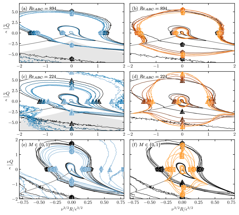
Figure 9: Joint histograms of the invariants $Q$ and $R$ of the fluid velocity gradient tensor. Panels (a) and (b) show cases with $Re_{ABC}=894$ for various particle mass fractions. Panels (c) and (d) show cases with $Re_{ABC}=224$ for various particle mass fractions. Panels (e) and (f) show fixed ($M=1$) and single-phase ($M=0$) cases for various Reynolds numbers. Numbered markers show the value of $\log p$ at each contour, where $p$ is the joint probability density function. The grey curve show where the discriminant is zero (equation 12). The grey shaded regions in the left panels are the loci of equation 13, where we observe an increase $p$ due to the presence of spheres.

The local topology of a flow can be described entirely using the three principle invariants of the velocity gradient tensor $\partial_{i}u_{j}$ [43]. The first invariant $\partial_{i}u_{i}$ is not interesting in our case because it is zero for an incompressible fluid. However, the second invariant $Q=\omega_{i}\omega_{i}/4-s_{ij}s_{ij}/2$ expresses the balance of vorticity and strain, while the third invariant $R=\omega_{i}s_{ij}\omega_{j}/4-s_{ij}s_{jk}s_{ki}/3$ is the balance of the production of vorticity with the production of strain [44]. The eigenvalues $\Lambda$ of $\partial_{i}u_{j}$ are the roots of the polynomial equation

$$\Lambda^{3}+Q\Lambda+R=0.$$ (12)

Figure 9 shows the joint probability distributions $p(R,Q)$ for all of our flows. We also plot a line where the discriminant of equation 12 is zero: $27R^{2}/4+Q^{3}=0$. Above this line $\partial_{i}u_{j}$ has one real and two complex eigenvalues and vortices dominate the flow. Below this line all three eigenvalues are real and the flow is dominated by strain. The single-phase distributions have tails in the top-left and bottom-right quadrants; these correspond to stretching vortices and regions where the flow compresses along one axis, respectively [43]. When spheres are added, both $Q$ and $R$ are reduced, as the non-slip boundary condition at their surfaces dampens the flow structures. Incidentally, a similar $Q$ and $R$ reduction has been seen with droplets [45]. However, we see that the addition of spheres causes $p(R,Q)$ to increase in the lower regions of the left panels in figure 9. This region is well-described by

$$27R^{2}/4+Q^{3}\lesssim-4\epsilon^{3}/\nu^{3}.$$ (13)

This region where spheres cause the probability distribution to increase corresponds to a strain-dominated flow. In fact, for pure strain, we have $Q=-s_{ij}s_{ij}/2$ and $R=0$. Hence we can substitute for $Q$ and $R$ in equation 13 to estimate that the dissipation is $2\nu s_{ij}s_{ij}\gtrsim 4^{4/3}\epsilon\approx 6\epsilon$ in the shear layers, i.e., the dissipation in the regions around the spheres is many times greater than the mean dissipation. Fibres also create shearing regions in the flow, seen by the increased probability density functions in the lower parts ($27R^{2}/4+Q^{3}<0$) of the right-hand panels in figure 9. As the fibre mass fraction is increased, the variance of $R$ is reduced, showing the production of strain and vorticity is suppressed by the fibres. At high fibre mass fractions the distributions are approximately symmetrical in $R$, in other words, $Q$ and $R$ are uncorrelated (much like the decorrelation of vorticity and strain observed for fibre-laden flows in figure 8). This suggests that the small fibre diameter produces many small scale structures which disrupt the typical turbulent flow. For both particle types, increasing the Reynolds number $Re_{ABC}$ reduces the effect of the particles.

IV Conclusion

We made simulations of finite-size isotropically- and anisotropically-shaped particles (spheres and fibres with size in the inertial range of scale) in turbulence at various Reynolds numbers and solid mass fractions. We used bulk flow statistics to show that particles reduce turbulence intensity relative to the single-phase case at all Reynolds numbers, with the fibres producing a more significant reduction effect than the spheres. From the trend in dissipation with Reynolds number, we see that the particle-laden flows behave like single-phase flows as $Re_{\lambda}\to\infty$, and the value of anomalous dissipation is $\epsilon\mathcal{L}/u^{\prime 3}\approx 0.4$ for both single-phase and particle-laden flows. However, spheres slow the convergence rate to the anomalous value, and fibres slow it further. Next, we analysed the flow at each scale of the simulation. Spheres and fibres provide a “spectral shortcut” to the flow, removing energy from the largest scales and injecting it at smaller scales. Spheres’ effect is mainly limited to the large scales, and they provide a spectral shortcut down to the length scale of their diameter. Fibres’ effect, on the other hand, occurs down to the length scale of the fibre thickness, even at low Reynolds numbers when it is deep in the viscous range ($d\ll\eta$). This shortcut of energy to the dissipative scales slows the dissipation’s convergence to its anomalous value as $Re_{\lambda}\to\infty$. Our scale-by-scale analysis also showed that particles cause the velocity field to become more intermittent in space. Multifractal spectra of the near-particle dissipation show that spheres enhance dissipation in two-dimensional sheets, and fibres enhance the dissipation in structures with a dimension greater than one and less than two. These lower dimensional structures are a possible source of intermittency in the flow. Zooming in closer to the flow, we looked at the shape of flow structures using their vorticity and shear. We saw that the particles enhance local shear, spheres suppress vortical flow structures, and fibres produce intense vortical and shearing structures, which overcome the usual vortex stretching behaviour. As Reynolds number increases, the flow structures created by the particles become less significant relative to the background turbulence.

To reiterate and answer our questions from section I; at what Reynolds numbers does turbulence modulation emerge? We see turbulence modulation at the lowest Reynolds number investigated $(Re_{\lambda}=12.8)$. This gives us reason to believe that particles modulate turbulence in even the most weakly turbulent flows $(Re_{\lambda}\to 0)$. Secondly, does the modulation effect persist as $Re\to\infty$? No, all of the statistics show a tendency towards single-phase results as $Re\to\infty$. Finally, how do the particle’s characteristic lengths impact the scales of the turbulent flow? Both spheres and particles take energy from the flow at scales larger than their size. Spheres re-inject energy around the characteristic length of their diameter, leaving the smaller scales relatively unperturbed, whereas fibres re-inject energy around the characteristic length of their thickness. The fibre thickness is at a small scale, so local flow structures are disrupted. None of the flow statistics shows any particular discerning feature at the length scale of the fibres.

These results relate to various environmental particle-laden flows, such as microplastics in the ocean, volcanic ash clouds, and sandstorms. We have explored the two extremes of isotropic and anisotropic particles, but further work is needed to investigate how intermediate aspect ratio particles such as ellipsoids interact with turbulent flows.

V Acknowledgements

The research was supported by the Okinawa Institute of Science and Technology Graduate University (OIST) with subsidy funding from the Cabinet Office, Government of Japan. The authors acknowledge the computer time provided by the Scientific Computing section of Research Support Division at OIST and the computational resources of the supercomputer Fugaku provided by RIKEN through the HPCI System Research Project (Project IDs: hp210229 and hp210269). SO acknowledges the support by grants FJC2021-047652-I and PID2022-142135NA-I00 by MCIN/AEI/10.13039/501100011033 and European Union NextGenerationEU/PRTR.

References

- Richardson and Proctor [1927] L. F. Richardson and D. Proctor, Diffusion over distances ranging from 3 km. to 86 km, Quarterly Journal of the Royal Meteorological Society 53, 149 (1927).
- Westerweel et al. [2013] J. Westerweel, G. E. Elsinga, and R. J. Adrian, Particle Image Velocimetry for Complex and Turbulent Flows, Annual Review of Fluid Mechanics 45, 409 (2013).
- Brizzolara et al. [2021] S. Brizzolara, M. E. Rosti, S. Olivieri, L. Brandt, M. Holzner, and A. Mazzino, Fiber Tracking Velocimetry for Two-Point Statistics of Turbulence, Physical Review X 11, 031060 (2021).
- Monchaux [2012] R. Monchaux, Measuring concentration with Voronoï diagrams: The study of possible biases, New Journal of Physics 14, 095013 (2012).
- Goto and Vassilicos [2008] S. Goto and J. C. Vassilicos, Sweep-Stick Mechanism of Heavy Particle Clustering in Fluid Turbulence, Physical Review Letters 100, 054503 (2008).
- Ireland et al. [2016] P. J. Ireland, A. D. Bragg, and L. R. Collins, The effect of Reynolds number on inertial particle dynamics in isotropic turbulence. Part 1. Simulations without gravitational effects, Journal of Fluid Mechanics 796, 617 (2016).
- Zhao et al. [2010] L. H. Zhao, H. I. Andersson, and J. J. J. Gillissen, Turbulence modulation and drag reduction by spherical particles, Physics of Fluids 22, 081702 (2010).
- Capecelatro et al. [2015] J. Capecelatro, O. Desjardins, and R. O. Fox, On fluid–particle dynamics in fully developed cluster-induced turbulence, Journal of Fluid Mechanics 780, 578 (2015).
- Olivieri et al. [2022a] S. Olivieri, I. Cannon, and M. E. Rosti, The effect of particle anisotropy on the modulation of turbulent flows, Journal of Fluid Mechanics 950, R2 (2022a).
- Brandt and Coletti [2021] L. Brandt and F. Coletti, Particle-Laden Turbulence: Progress and Perspectives, Annual Review of Fluid Mechanics 54, 10.1146/annurev-fluid-030121-021103 (2021).
- Wadell [1932] H. Wadell, Volume, Shape, and Roundness of Rock Particles, The Journal of Geology 40, 443 (1932).
- Paschkewitz et al. [2004] J. S. Paschkewitz, Y. Dubief, C. D. Dimitropoulos, E. S. G. Shaqfeh, and P. Moin, Numerical simulation of turbulent drag reduction using rigid fibres, Journal of Fluid Mechanics 518, 281 (2004).
- Gillissen et al. [2008] J. J. J. Gillissen, B. J. Boersma, P. H. Mortensen, and H. I. Andersson, Fibre-induced drag reduction, Journal of Fluid Mechanics 602, 209 (2008).
- Zhao et al. [2015] L. Zhao, N. R. Challabotla, H. I. Andersson, and E. A. Variano, Rotation of Nonspherical Particles in Turbulent Channel Flow, Physical Review Letters 115, 244501 (2015).
- Bounoua et al. [2018] S. Bounoua, G. Bouchet, and G. Verhille, Tumbling of Inertial Fibers in Turbulence, Physical Review Letters 121, 124502 (2018).
- Yousefi et al. [2020] A. Yousefi, M. N. Ardekani, and L. Brandt, Modulation of turbulence by finite-size particles in statistically steady-state homogeneous shear turbulence, Journal of Fluid Mechanics 899, A19 (2020).
- Ardekani et al. [2017] M. N. Ardekani, P. Costa, W.-P. Breugem, F. Picano, and L. Brandt, Drag reduction in turbulent channel flow laden with finite-size oblate spheroids, Journal of Fluid Mechanics 816, 43 (2017).
- Voth and Soldati [2017] G. A. Voth and A. Soldati, Anisotropic Particles in Turbulence, Annual Review of Fluid Mechanics 49, 249 (2017).
- Lucci et al. [2010] F. Lucci, A. Ferrante, and S. Elghobashi, Modulation of isotropic turbulence by particles of Taylor length-scale size, Journal of Fluid Mechanics 650, 5 (2010).
- Oka and Goto [2022] S. Oka and S. Goto, Attenuation of turbulence in a periodic cube by finite-size spherical solid particles, Journal of Fluid Mechanics 949, A45 (2022).
- Peng et al. [2023] C. Peng, Q. Sun, and L.-P. Wang, Parameterization of turbulence modulation by finite-size solid particles in forced homogeneous isotropic turbulence, Journal of Fluid Mechanics 963, A6 (2023).
- Shen et al. [2022] J. Shen, C. Peng, J. Wu, K. L. Chong, Z. Lu, and L.-P. Wang, Turbulence modulation by finite-size particles of different diameters and particle–fluid density ratios in homogeneous isotropic turbulence, Journal of Turbulence 23, 433 (2022).
- Libin and Sivashinsky [1990] A. Libin and G. Sivashinsky, Long wavelength instability of the ABC-flows, Quarterly of Applied Mathematics 48, 611 (1990).
- Podvigina and Pouquet [1994] O. Podvigina and A. Pouquet, On the non-linear stability of the 1:1:1 ABC flow, Physica D: Nonlinear Phenomena 75, 471 (1994).
- Kim and Moin [1985] J. Kim and P. Moin, Application of a fractional-step method to incompressible Navier-Stokes equations, Journal of Computational Physics 59, 308 (1985).
- Hori et al. [2022] N. Hori, M. E. Rosti, and S. Takagi, An Eulerian-based immersed boundary method for particle suspensions with implicit lubrication model, Computers & Fluids 236, 105278 (2022).
- Huang et al. [2007] W.-X. Huang, S. J. Shin, and H. J. Sung, Simulation of flexible filaments in a uniform flow by the immersed boundary method, Journal of Computational Physics 226, 2206 (2007).
- Alizad Banaei et al. [2020] A. Alizad Banaei, M. E. Rosti, and L. Brandt, Numerical study of filament suspensions at finite inertia, Journal of Fluid Mechanics 882, A5 (2020).
- Olivieri et al. [2020] S. Olivieri, L. Brandt, M. E. Rosti, and A. Mazzino, Dispersed Fibers Change the Classical Energy Budget of Turbulence via Nonlocal Transfer, Physical Review Letters 125, 114501 (2020).
- Yu [2005] Z. Yu, A DLM/FD method for fluid/flexible-body interactions, Journal of Computational Physics 207, 1 (2005).
- Snook et al. [2012] B. Snook, E. Guazzelli, and J. E. Butler, Vorticity alignment of rigid fibers in an oscillatory shear flow: Role of confinement, Physics of Fluids 24, 121702 (2012).
- Shaik and Van Hout [2023] S. Shaik and R. Van Hout, Kinematics of rigid fibers in a turbulent channel flow, International Journal of Multiphase Flow 158, 104262 (2023).
- Donzis et al. [2005] D. A. Donzis, K. R. Sreenivasan, and P. K. Yeung, Scalar dissipation rate and dissipative anomaly in isotropic turbulence, Journal of Fluid Mechanics 532, 199 (2005).
- Taylor [1935] G. I. Taylor, Statistical Theory of Turbulence, Proceedings of the Royal Society of London. Series A, Mathematical and Physical Sciences 151, 421 (1935), 96557 .
- Doering and Foias [2002] C. R. Doering and C. Foias, Energy dissipation in body-forced turbulence, Journal of Fluid Mechanics 467, 289 (2002).
- Abdelgawad* et al. [2023] M. S. Abdelgawad*, I. Cannon*, and M. E. Rosti, Scaling and intermittency in turbulent flows of elastoviscoplastic fluids, Nature Physics , 1 (2023).
- Finnigan [2000] J. Finnigan, Turbulence in Plant Canopies, Annual Review of Fluid Mechanics 32, 519 (2000).
- Pope [2000] S. B. Pope, Turbulent Flows (Cambridge University Press, 2000).
- Frisch [1995] U. Frisch, Turbulence: The Legacy of A. N. Kolmogorov (Cambridge University Press, 1995).
- Mukherjee et al. [2023] S. Mukherjee, S. D. Murugan, R. Mukherjee, and S. S. Ray, Turbulent flows are not uniformly multifractal (2023), arxiv:2307.06074 .
- Ashurst et al. [1987] Wm. T. Ashurst, A. R. Kerstein, R. M. Kerr, and C. H. Gibson, Alignment of vorticity and scalar gradient with strain rate in simulated Navier–Stokes turbulence, The Physics of Fluids 30, 2343 (1987).
- Olivieri et al. [2022b] S. Olivieri, A. Mazzino, and M. E. Rosti, On the fully coupled dynamics of flexible fibres dispersed in modulated turbulence, Journal of Fluid Mechanics 946, A34 (2022b).
- Cheng and Cantwell [1996] W.-P. Cheng and B. Cantwell, Study of the Velocity Gradient Tensor in Turbulent Flow, Tech. Rep. JIAA TR 114 (1996).
- Paul et al. [2022] I. Paul, B. Fraga, M. S. Dodd, and C. C. K. Lai, The role of breakup and coalescence in fine-scale bubble-induced turbulence. II. Kinematics, Physics of Fluids 34, 083322 (2022).
- Perlekar [2019] P. Perlekar, Kinetic energy spectra and flux in turbulent phase-separating symmetric binary-fluid mixtures, Journal of Fluid Mechanics 873, 459 (2019).