RandCom: Random Communication Skipping Method
for Decentralized Stochastic Optimization

Abstract

Distributed optimization methods with random communication skips are gaining increasing attention due to their proven benefits in accelerating communication complexity. Nevertheless, existing research mainly focuses on centralized communication protocols for strongly convex deterministic settings. In this work, we provide a decentralized optimization method called RandCom, which incorporates probabilistic local updates. We analyze the performance of RandCom in stochastic non-convex, convex, and strongly convex settings and demonstrate its ability to asymptotically reduce communication overhead by the probability of communication. Additionally, we prove that RandCom achieves linear speedup as the number of nodes increases. In stochastic strongly convex settings, we further prove that RandCom can achieve linear speedup with network-independent stepsizes. Moreover, we apply RandCom to federated learning and provide positive results concerning the potential for achieving linear speedup and the suitability of the probabilistic local update approach for non-convex settings.

1 Introduction

In this work, we consider the following stochastic optimization problem in a decentralized setting:

$$f^{\star}=\min_{{\bf{x}}\in\mathbb{R}^{d}}\Big{[}f({\bf{x}}):=\frac{1}{n}\sum_{i=1}^{n}f_{i}({\bf{x}})\Big{]},$$ (1)

$$\text{with }f_{i}({\bf{x}})=\mathbb{E}_{\xi_{i}\sim\mathcal{D}_{i}}[F_{i}({\bf{x}},\xi_{i})],$$

where$\{\mathcal{D}_{i}\}^{n}_{i=1}$ represent data distributions, which can be heterogeneous across $n$ nodes, $f_{i}:\mathbb{R}^{d}\rightarrow\mathbb{R}$ is a smooth local function accessed by node $i$. This problem carries significant importance as it serves as an abstraction of empirical risk minimization, the prevailing framework in supervised machine learning and gaming. Solving problem (1) in a decentralized manner has garnered considerable attention in recent years [1, 2, 3]. The motivation behind these efforts stems from the potential of decentralization to eliminate the need for data sharing and centralized synchronization, and to mitigate the high latency that is commonly encountered in centralized computing architectures [4]. Nevertheless, decentralized optimization algorithms may still face challenges arising from communication bottlenecks.

To reduce communication costs in distributed training, many techniques have been proposed. These techniques include compressing models and gradients [5], using asynchronous communication [6], and implementing local updates [7]. By applying these strategies, it is possible to reduce the amount of information exchanged between different nodes during training, thereby improving the efficiency of distributed training setups. In this work, we mainly focus on performing local updates as means to reduce communication frequency. Although this approach has demonstrated considerable practical advantages, it is still difficult to analyse theoretically.

In centralized settings, local-SGD/FedAvg [7, 8, 9] has emerged as one of the most widely adopted learning methods that employ local updates. However, when dealing with heterogeneous data, Local-SGD/FedAvg encounters the challenge of “client-drift.” This phenomenon arises from the diversity of functions on each node, causing each client to converge towards the minima of its respective function $f_{i}$, which may be significantly distant from the global optimum $f^{\star}$. To tackle this issue, several algorithms have been proposed, including Scaffold [10], FedLin [11], FedPD [12], Scaffnew [13], TAMUNA [14], and CompressedScaffnew [15].

Table 1: A comparison with existing methods employing local steps. The notation $\tilde{\mathcal{O}}(\cdot)$ ignores logarithmic factors. NC, C, and SC denote Non-Convex, Convex and Strongly Convex, respectivel; ComAcc denotes communication acceleration, INP denotes Independent of Network Topology, SCS denotes Stochastic Communication Skips, and Dec denotes Decentralized.

Method	# communication rounds		ComAcc $|$ stepsize	linear speedup	Dec	SCS
	NC/C	SC	SC, $\sigma=0$	NC $|$ C $|$ SC (INP)
Scaffold [10]	$\mathcal{O}\left(\frac{\sigma^{2}}{nK\epsilon^{2}}+\frac{1}{\epsilon}\right)$	$\tilde{\mathcal{O}}\left(\frac{\sigma^{2}}{nK\epsilon}+\mathrm{log}\nicefrac{{1}}{{\epsilon}}\right)$	✗ $|$ $\mathcal{O}\left(\frac{1}{KL}\right)$	✓ $|$ ✓ $|$ ✗	✗	✗
Scaffnew [13]	no results	$\tilde{\mathcal{O}}\left(\frac{p\sigma^{2}}{\epsilon}+p\mathrm{log}\nicefrac{{1}}{{\epsilon}}\right){\textsuperscript{a}}$	✓ $|$ $\mathcal{O}\left(\frac{1}{L}\right)$	no results	✗	✓
local-DSGD [16]	$\mathcal{O}\left(\frac{p\sigma^{2}}{n\epsilon^{2}}+\left(\frac{\sigma\sqrt{p}}{\sqrt{\rho}}+\frac{\varsigma}{\rho}\right)\frac{1}{\epsilon^{\nicefrac{{3}}{{2}}}}+\frac{1}{\rho\epsilon}\right)$b	$\tilde{\mathcal{O}}\left(\frac{p\sigma^{2}}{n\epsilon}+\left(\frac{\sigma\sqrt{p}}{\sqrt{\rho}}+\frac{\varsigma}{\rho}\right)\frac{1}{\sqrt{\epsilon}}+\frac{1}{\rho}\mathrm{log}\nicefrac{{1}}{{\epsilon}}\right)$	✗ $|$ $\mathcal{O}\big{(}\frac{p\rho}{L}\big{)}$	✓ $|$ ✓ $|$ ✗	✓	✓
$K$-GT[18]	$\mathcal{O}\left(\frac{\sigma^{2}}{nK\epsilon^{2}}+\left(\frac{\sigma}{\rho^{2}\sqrt{K}}\right)\frac{1}{\epsilon^{\nicefrac{{3}}{{2}}}}+\frac{1}{\rho^{2}\epsilon}\right){\textsuperscript{c}}$	no results	✗ $|$ no results	✓ $|$ ✗ $|$ ✗	✓	✗
LED [19]	$\mathcal{O}\left(\frac{\sigma^{2}}{nK\epsilon^{2}}+\left(\frac{\sigma}{\sqrt{\rho K}}\right)\frac{1}{\epsilon^{\nicefrac{{3}}{{2}}}}+\frac{1}{\rho\epsilon}\right)$	$\tilde{\mathcal{O}}\left(\frac{\sigma^{2}}{nK\epsilon}+\left(\frac{\sigma}{\sqrt{\rho K}}\right)\frac{1}{\sqrt{\epsilon}}+\frac{1}{\rho}\mathrm{log}\nicefrac{{1}}{{\epsilon}}\right)$	✗ $|$ $\mathcal{O}\left(\frac{\rho}{KL}\right)$	✓ $|$ ✓ $|$ ✗	✓	✗
D-Scaffnew [13]	no results	no results	✓ $|$ $\mathcal{O}\left(\frac{1}{L}\right)$	no results	✓	✓
RandProx [20]	no results	no results	✓ $|$ $\mathcal{O}\left(\frac{1}{L}\right)$	no results	✓	✓
RandCom d	$\mathcal{O}\left(\frac{p\sigma^{2}}{n\epsilon^{2}}+\left(\frac{\sigma p}{\sqrt{\rho}}\right)\frac{1}{\epsilon^{\nicefrac{{3}}{{2}}}}+\frac{p}{\rho\epsilon}\right)$	$\tilde{\mathcal{O}}\left(\frac{p\sigma^{2}}{n\epsilon}+\left(\frac{\sigma p}{\sqrt{\rho}}\right)\frac{1}{\sqrt{\epsilon}}+\frac{p}{\rho}\mathrm{log}\nicefrac{{1}}{{\epsilon}}\right)$	✓ $|$ $\mathcal{O}\left(\frac{1}{L}\right)$	✓ $|$ ✓ $|$ ✓	✓	✓

• The complexity can be derived from [13, Theorem 5.5] and [19, Corollary 1] ([16, Lemma 15]) and $p\in[\sqrt{\alpha\mu},1]$.

• $\rho=1-\lambda_{2}$, where $\lambda_{2}$ is the mixing rate of the network (for fully connected network $\rho=1$), $\sigma$ is the stochastic gradient
  noise, and $\varsigma$ is function heterogeneity constant such that $\nicefrac{{1}}{{n}}\sum_{i=1}^{n}\|\nabla f_{i}({\bf{x}})\|^{2}\leq\varsigma^{2}+B^{2}\|\nabla f({\bf{x}})\|^{2}$, with $B\geq 1$.

• This is the communication complexity in stochastic non-convex settings, and no corresponding result is given in [18] in
  stochastic convex settings.

• In RandCom, we assume that $p\in[\nicefrac{{1}}{{\chi}},1]\cap[1-\rho,1]$.

In decentralized settings, local-DSGD has been introduced in [16]. Similarly to local-SGD, it also encounters the issue of client-drift when dealing with heterogeneous data. To mitigate the drift in Local-DSGD, several algorithms have been proposed, including Local Gradient-Tracking (local-GT) [17], $K$-GT [18], LED [19], D-Scaffnew [13], and RandProx [20]. Although local-GT [17] provides performance analysis in non-convex settings, it is limited to deterministic scenarios. The works $K$-GT [18] and LED [19] explore the performance in stochastic (strongly) convex and/or non-convex settings. However, these methods [16, 17, 18, 19] incorporate deterministic periodic local updates and their theoretical communication complexity remains unchanged. Specifically, for LED [19], assuming that $f_{i}$ is $\mu$-strongly convex and $L$-smooth, and $f_{i}$ is deterministic, the communication complexity is still $\mathcal{O}\left(\kappa\kappa_{w}\mathrm{log}\ \epsilon^{-1}\right)$, where $\kappa=\nicefrac{{L}}{{\mu}}$ represents the condition number of $f_{i}$, and $\kappa_{w}$ is the condition number of the communication network. Furthermore, the stepsize is $\mathrm{O}\left(\nicefrac{{1}}{{KL}}\right)$, where $K$ denotes the number of local updates. This implies that more local updates result in smaller step sizes, which impacts the convergence rate. In contrast, D-Scaffnew [13] and RandProx [20], which examine probabilistic local updates or communication skipping, surpass this communication complexity barrier and achieves the optimal communication complexity of $\mathcal{O}\left(\sqrt{\kappa\kappa_{w}}\ \mathrm{log}\nicefrac{{1}}{{\epsilon}}\right)$ [22], without relying on classical acceleration schemes. Moreover, the stepsize is $\mathcal{O}\left(\nicefrac{{1}}{{L}}\right)$, which remains independent of the number of local updates. However, D-Scaffnew [13] and RandProx [20] solely analyse performance in strongly convex scenarios, and for stochastic settings, the analysis does not show linear speedup in the number of nodes $n$.

For the stochastic decentralized problem (1), this paper introduces a novel decentralized algorithm named RandCom (Randomized Communication), drawing inspiration from [13, 19, 20], and provides convergence analysis in stochastic non-convex, convex, and strongly convex settings. We conduct a comparative analysis of RandCom with existing methods that utilize local steps, and the results are summarized in Table 1. The main contributions of this paper are outlined below.

• In this study, we introduce a novel algorithm for decentralized stochastic convex and nonconvex optimization problems (1) that incorporates probabilistic local updates, where communication occurs with a probability of $p$. This distinguishes our approach from previous works [16, 17, 18, 19] that focus on periodic local updates. Additionally, compared to them, we obtain a provable communication acceleration by $p$ in deterministic cases (refer to Table 1).

• In the stochastic non-convex, convex, and strongly convex settings, we establish the convergence of RandCom. Our rates are comparable to the best existing decentralized and centralized bounds (refer to Table 1). After enough transient time, the expected communication complexity of RandCom is $\mathcal{O}\big{(}\frac{p\sigma^{2}}{n\epsilon^{2}}\big{)}$ ($\mathcal{O}\big{(}\frac{p\sigma^{2}}{n\epsilon}\big{)}$ for strongly convex case), where $\sigma^{2}$ represents the level of stochastic noise and $\epsilon$ denotes the desired accuracy level. This result demonstrates that RandCom achieves linear speedup with respect to the probability of communication $p$ and the number of nodes $n$.

• In the stochastic strongly convex settings, similar to [21], we further prove that RandCom achieves linear speedup by $n$ with stepsizes that are independent of the network structure. For deterministic gradient settings, we illustrate that RandCom inherits the advantages of D-Scaffnew [13] in achieving reliable communication acceleration.

• We explore the application of RandCom in the context of federated learning. Prior to this study, there was no results demonstrating the convergence of federated learning methods in non-convex settings or with linear speedup using probabilistic local updates. In this research, we demonstrate that these outcomes can indeed be achieved.

This paper is organized as follows. In Section 2, we introduce the proposed RandCom and investigate the application in the context of federated learning. Moreover, we present a new perspective on the construction of RandCom and relate it to existing algorithms. In Section 3, we give our main theoretical results. Finally, several numerical simulations are implemented in Section 4 and conclusions are given in Section 5.

2 The Proposed Algorithm: RandCom

All vectors are column vectors unless otherwise stated. Let $\mathbf{x}_{i}^{t}\in\mathbb{R}^{d}$ represent the local state of node $i$ at the $t$-th iteration. For the sake of convenience in notation, we use bold capital letters to denote stacked variables. For instance,

$$\mathbf{X}^{t}:= \ [\mathbf{x}_{1}^{t},\mathbf{x}_{2}^{t},\ldots,\mathbf{x}_{n}^{t}]^{\sf T}\in\mathbb{R}^{n\times d},$$

$$\mathbf{G}^{t}:= \ [\mathbf{g}_{1}^{t},\mathbf{g}_{2}^{t},\ldots,\mathbf{g}_{n}^{t}]^{\sf T}\in\mathbb{R}^{n\times d},$$

$$\nabla F(\mathbf{X}^{t}):= \ [\nabla f_{1}(\mathbf{x}^{t}_{1}),\nabla f_{2}(\mathbf{x}^{t}_{2}),\ldots,\nabla f_{n}(\mathbf{x}^{t}_{n})]^{\sf T}\in\mathbb{R}^{n\times d}.$$

2.1 Network Graph

In this work, we focus on decentralized scenarios, where a network of $n$ nodes is interconnected by a graph with a set of edges $\mathcal{E}$, where node $i$ is connected to node $j$ of $(i,j)\in\mathcal{E}$. To describe the algorithm, we introduce the global mixing matrix $\mathbf{W}=[W_{ij}]$, where $W_{ij}=W_{ji}=0$ if $(i,j)\notin\mathcal{E}$, and $W_{ij}>0$ otherwise. We impose the following standard assumption on the mixing matrix.

Assumption 1.

The mixing matrix $\mathbf{W}\in[0,1]^{n\times n}$ is symmetric and doubly stochastic. Let $\lambda_{1}=1$ denote the largest eigenvalue of the mixing matrix $\mathbf{W}$, and the remaining eigenvalues are denoted as $1>\lambda_{2}\geq\lambda_{3}\geq\cdots\geq\lambda_{n}>-1$.

We introduce two quantities as follows:$\mathbf{W}_{a}=\mathbf{I}-\nicefrac{{1}}{{2\chi}}(\mathbf{I}-\mathbf{W}),\ \mathbf{W}_{b}=(\mathbf{I}-\mathbf{W})^{1/2}$, where $\chi\geq 1$. Under Assumption 1, it can be shown that $\mathbf{W}_{a}$ is positive semi-definite and doubly stochastic. Furthermore, we have $\mathbf{I}-\mathbf{W}_{a}=\nicefrac{{1}}{{2\chi}}\mathbf{W}_{b}^{2}$, and $\mathbf{W}_{a}$ is well-conditioned when $\chi$ is large. By noting that $\|\mathbf{W}_{b}^{2}\|<2$, we define the condition number of the communication network as $\kappa_{w}=\nicefrac{{1}}{{1-\lambda_{2}}}$, which upper bounds the ratio between the largest eigenvalue and the smallest non-zero eigenvalue of $\nicefrac{{1}}{{2}}\mathbf{W}_{b}^{2}$.

Algorithm 1 RandCom for decentralized learning

1:  Input $\alpha>0$, $\beta>0$, $0<p\leq 1$, $\chi\geq 1$, initial iterates ${\bf{x}}^{0}_{i}={\bf{x}}^{0}\in\mathbb{R}^{d},~{}i=1,\dots,n$, initial dual variables ${\bf{y}}^{0}_{i}=0,~{}i=1,\dots,n$, weights for averaging ${\bf{W}}_{a}={\bf{I}}-\nicefrac{{1}}{{2\chi}}({\bf{I-W}}):=(\widetilde{W}_{ij})^{n}_{i,j=1}$.

2:  for $t=0,1,\dotsc,T-1$ do

3:     Flip a coin $\theta_{t}\in\{0,1\}$, $\mathop{\rm Prob}(\theta_{t}=1)=p$

4:     for $i=1,\dotsc,n$ do

5:        Sample $\xi_{i}^{t}$, compute gradient ${\bf{g}}_{i}^{t}=\nabla F_{i}({\bf{x}}^{t}_{i},\xi^{t}_{i})$

6:        $\hat{{\bf{z}}}^{t}_{i}={\bf{x}}^{t}_{i}-\alpha{\bf{g}}^{t}_{i}-{\bf{y}}^{t}_{i}$ $\triangleright$ Update the prediction variate $\hat{{\bf{z}}}^{t}_{i}$

7:        if $\theta_{t}=1$ then

8:           ${\bf{x}}^{t+1}_{i}=\sum_{j=1}^{n}\widetilde{W}_{ij}\hat{{\bf{z}}}^{t}_{j}$ $\triangleright$ Communicate with prob $p$

9:           ${\bf{y}}^{t+1}_{i}={\bf{y}}^{t}_{i}+\beta(\hat{{\bf{z}}}^{t}_{i}-{\bf{x}}^{t+1}_{i})$ $\triangleright$ Update the control variate ${\bf{y}}^{t+1}_{i}$

10:        else

11:           ${\bf{y}}^{t+1}_{i}={\bf{y}}^{t}_{i},~{}{\bf{x}}^{t+1}_{i}=\hat{{\bf{z}}}^{t}_{i}$ $\triangleright$ Skip communication

12:        end if

13:     end for

14:  end for

2.2 Algorithm Description

With Assumption 1, the constraint $\mathbf{x}_{1}=\mathbf{x}_{2}=\cdots=\mathbf{x}_{n}$ is equivalent to $\mathbf{W}_{b}\mathbf{X}=0$. Then, the problem (1) can be reformulated as

$$\min_{{\bf{X}}\in\mathbb{R}^{n\times d}}~{}F({\bf{X}}):=\frac{1}{n}\sum_{i=1}^{n}f_{i}({\bf{x}}_{i}),~{}\mathrm{s.t.~{}}{\bf{W}}_{b}\mathbf{X}=0.$$ (2)

By incorporating probabilistic local updates, which is a commonly employed technique for reducing communication overhead [13], we propose RandCom as a solution to problem (2) with the following update scheme:

$$\hat{\mathbf{Z}}^{t} =\mathbf{X}^{t}-\alpha\mathbf{G}^{t}-\mathbf{Y}^{t},$$ (3a)

$$\mathbf{X}^{t+1} =(1-\theta_{t})\hat{\mathbf{Z}}^{t}+\theta_{t}\mathbf{W}_{a}\hat{\mathbf{Z}}^{t},$$ (3b)

$$\mathbf{Y}^{t+1} =\mathbf{Y}^{t}+\beta(\hat{\mathbf{Z}}^{t}-\mathbf{X}^{t+1}).$$ (3c)

Here, $\alpha>0$ is the stepsize (learning rate), $\beta>0$, $\mathbf{G}^{t}=[\mathbf{g}_{1}^{t},\mathbf{g}_{2}^{t},\ldots,\mathbf{g}_{n}^{t}]^{\sf T}\in\mathbb{R}^{n\times d}$ with $\mathbf{g}_{i}^{t}$ representing the stochastic gradient of $\nabla f_{i}(\mathbf{x}_{i}^{t})$, $\theta_{t}=1$ with probability $p$ and $\theta_{t}=0$ with probability $1-p$, and $\mathbf{Y}^{t}$ is the control variate. At each iteration $t\geq 0$, communication takes place with a probability $p\in(0,1]$. In the absence of communication, the update $\mathbf{X}^{t+1}=\mathbf{X}^{t}-\alpha\mathbf{G}^{t}-\mathbf{Y}^{t}$ is performed, while $\mathbf{Y}^{t+1}$ remains unchanged. This allows for multiple iterations of local computations to be performed between communication rounds. By decomposing the updates for individual nodes, we provide a detailed implementation of RandCom (3) in Algorithm 1.

2.3 RandCom for Federated Learning

In this subsection, we investigate the application of RandCom in the context of federated learning, which can also be formulated as problem (1) and equivalently transformed to problem (2). Unlike the decentralized setting, federated learning involves parallel computing units that possess private data stored on each unit. These units communicate with a remote orchestrating server, which aggregates the information and coordinates the computations to achieve consensus and converge towards a globally optimal model.

To this end, we consider the mixing matrix ${\bf{W}}=\nicefrac{{1}}{{n}}{\bf{1}}{\bf{1}}^{\sf T}$, which leads to the following algorithms:

$$\hat{{\bf{Z}}}^{t} =\ {\bf{X}}^{t}-\alpha{\bf{G}}^{t}-{\bf{Y}}^{t},$$ (4a)

$${\bf{X}}^{t+1} =\ (1-\theta_{t})\hat{{\bf{Z}}}^{t}+\frac{\theta_{t}(2\chi-1)}{2\chi}\hat{{\bf{Z}}}^{t}+\frac{\theta_{t}}{2n\chi}{\bf{1}}{\bf{1}}^{\sf T}\hat{{\bf{Z}}}^{t},$$ (4b)

$${\bf{Y}}^{t+1} =\ {\bf{Y}}^{t}+\beta(\hat{{\bf{Z}}}^{t}-{\bf{X}}^{t+1}).$$ (4c)

By separating the updates between the clients and the server, we provide the detailed implementation of RandCom for federated learning in Algorithm 2. This method has three main steps: local updates to the client model $\hat{{\bf{z}}}^{t}_{i}$, local updates to the client control variate $\hat{{\bf{y}}}^{t}_{i}$, and averaging the client models with probability $p$ in every iteration.

Algorithm 2 RandCom for federated learning

1:  Input $\alpha>0$, $\beta>0$, $0<p\leq 1$, initial iterates ${\bf{x}}^{0}_{i}={\bf{x}}^{0}\in\mathbb{R}^{d},~{}i=1,\dots,n$, initial dual variables ${\bf{y}}^{0}_{i}=0,~{}i=1,\dots,n$, number of iterations $T\geq 1$.

2:  for $t=0,1,\dotsc,T-1$ do

3:     Server: Flip a coin $\theta_{t}\in\{0,1\}$, $\mathop{\rm Prob}(\theta_{t}=1)=p$ $\triangleright$ Decide when to skip communication

4:     for $i=1,\dotsc,n$ at clients in parallel do

5:        Sample $\xi_{i}^{t}$, compute gradient ${\bf{g}}_{i}^{t}=\nabla F_{i}({\bf{x}}^{t}_{i},\xi^{t}_{i})$

6:        $\hat{{\bf{z}}}^{t}_{i}={\bf{x}}^{t}_{i}-\alpha{\bf{g}}^{t}_{i}-{\bf{y}}^{t}_{i}$ $\triangleright$ Update the prediction variate $\hat{{\bf{z}}}^{t}_{i}$

7:        if $\theta_{t}=1$ then

8:           send $\hat{{\bf{z}}}^{t}_{i}$ to the server, which aggregates $\bar{{\bf{x}}}_{c}^{t+1}=\frac{1}{n}\sum_{j=1}^{n}\hat{{\bf{z}}}^{t}_{j}$ and broadcasts it to all clients

9:           ${\bf{x}}^{t+1}_{i}=\hat{{\bf{z}}}^{t}_{i}+\nicefrac{{1}}{{2\chi}}(\bar{{\bf{x}}}_{c}^{t+1}-\hat{{\bf{z}}}^{t}_{i})$

10:           ${\bf{y}}^{t+1}_{i}={\bf{y}}^{t}_{i}+\nicefrac{{\beta}}{{2\chi}}(\hat{{\bf{z}}}^{t}_{i}-\bar{{\bf{x}}}_{c}^{t+1})$ $\triangleright$ Update the control variate ${\bf{y}}^{t+1}_{i}$

11:        else

12:           ${\bf{y}}^{t+1}_{i}={\bf{y}}^{t}_{i},~{}{\bf{x}}^{t+1}_{i}=\hat{{\bf{z}}}^{t}_{i}$ $\triangleright$ Skip communication

13:        end if

14:     end for

15:  end for

It is important to mention that when $\chi=\nicefrac{{1}}{{2}}$ and $\beta=p$, RandCom simplifies to Scaffnew [13]. In this case, (4c) becomes:

$${\bf{X}}^{t+1}=\ (1-\theta_{t})\hat{{\bf{Z}}}^{t}+\frac{\theta_{t}}{n}{\bf{1}}{\bf{1}}^{\sf T}\hat{{\bf{Z}}}^{t}$$

$$\Rightarrow{\bf{x}}_{i}^{t+1}=\ (1-\theta_{t})\hat{{\bf{z}}}_{i}^{t}+\frac{\theta_{t}}{n}\sum_{j=1}^{n}\hat{{\bf{z}}}_{j}^{t},\ i=1,\dots,n.$$

However, it is important to note that the analysis techniques presented in [13] do not demonstrate linear speedup and are limited to the specific case of strongly-convex costs. In contrast, RandCom can achieve linear speedup and is applicable to non-convex settings.

2.4 Discussion

In this subsection, we present the motivation behind RandCom and relate it to existing algorithms, which incorporate probabilistic local updates.

New perspective on the construction of RandCom: We now provide a new perspective on RandCom in terms of operator splitting. Recall problem (2), which is equivalent to

$$\min_{{\bf{X}}}F({\bf{X}})+\delta_{{0}}({\bf{W}}_{b}{\bf{X}}),$$ (5)

where $\delta_{{0}}({\bf{W}}_{b}{\bf{X}})$ is an indicator function defined as $\delta_{{0}}({\bf{W}}_{b}{\bf{X}})=0$ if ${\bf{W}}_{b}{\bf{X}}=0$; otherwise, $\delta_{{0}}({\bf{W}}_{b}{\bf{X}})=\infty$, which enforces the constraint ${\bf{W}}_{b}{\bf{X}}=0$. For brevity, we define the following operators:

$$\bm{A}=\left[\begin{array}[]{cc}0&{\bf{W}}_{b}\\ -{\bf{W}}_{b}&0\\ \end{array}\right],\ \bm{B}=\left[\begin{array}[]{cc}\nabla F&0\\ 0&0\\ \end{array}\right],\bm{Q}_{1}=\left[\begin{array}[]{cc}\frac{1}{\alpha}{\bf{I}}&-{\bf{W}}_{b}\\ 0&2\alpha\chi{\bf{I}}\\ \end{array}\right],\ \bm{Q}_{2}=\left[\begin{array}[]{cc}{\bf{I}}&-\alpha{\bf{W}}_{b}\\ 0&{\bf{I}}\\ \end{array}\right].$$

For any $({\bf{X}}^{\star},{\bf{U}}^{\star})$ such that $(\bm{A+B})({\bf{X}}^{\star},{\bf{U}}^{\star})=0$, ${\bf{X}}^{\star}$ is a solution to (5) and ${\bf{U}}^{\star}$ is a solution to its dual problem. Let $(\hat{{\bf{Z}}}^{t},{\bf{U}}^{t+1})=\tilde{\bm{K}}^{t}$ and $({\bf{X}}^{t+1},{\bf{U}}^{t+1})=\bm{K}^{t+1}$. When $p=1$, $\beta=1$, ${\bf{G}}^{t}=\nabla F({\bf{X}}^{t})$, and ${\bf{Y}}^{t}=\alpha{\bf{W}}_{b}{\bf{U}}^{t}$, RandCom can be viewed as a triangularly preconditioned forward-backward operator splitting algorithm with a primal corrector. It aims to find the zero point of $\bm{A}+\bm{B}$. Specifically, RandCom (3) can be rewritten as follows:

$$\tilde{\bm{K}}^{t} =(\bm{Q}_{1}+\bm{A})^{-1}(\bm{Q}_{1}-{\bf{B}})\bm{K}^{t},$$

$$\bm{K}^{t+1} =\bm{K}^{t}-\bm{Q}_{2}(\bm{K}^{t}-\tilde{\bm{K}}^{t}).$$

Upon closer examination of the update equation (43), we can observe that RandCom can be regarded as a specific instance of RandProx [20]. RandProx, in turn, serves as a generalization of the PDDY algorithm [25], which utilizes the Davis-Yin splitting [26] technique to address a monotone inclusion problem within a primal-dual product space, incorporating a stochastic skipping of the proximity operator. However, in contrast to these approaches, we offer a fresh perspective on the construction of RandCom, providing a novel and unique viewpoint on the methodology employed in our proposed algorithm.

Relation with D-Scaffnew [13]: Recall the update of D-Scaffnew [13]:

$$\hat{{\bf{Z}}}^{t} =\ {\bf{X}}^{t}-\alpha{\bf{G}}^{t}-{\bf{Y}}^{t},$$

$${\bf{X}}^{t+1} =\ (1-\theta_{t})\hat{{\bf{Z}}}^{t}+\theta_{t}\big{(}{\bf{I}}-\tfrac{\alpha\tau}{p}\left({\bf{I-W}}\right)\big{)}\hat{{\bf{Z}}}^{t},$$

$${\bf{Y}}^{t+1} =\ {\bf{Y}}^{t}+p(\hat{{\bf{Z}}}^{t}-{\bf{X}}^{t+1}),$$

where $\tau>0$ and satisfies that $\alpha\tau\|{\bf{I-W}}\|\leq p$. Compared to RandCom (3), when $\beta=p$, the main difference is the choice of the parameter $\tau$ (or $\chi$). To better expose this, let us compare them as follows.

RandCom: $${\bf{X}}^{t+1}=\ (1-\theta_{t})\hat{{\bf{Z}}}^{t}+\theta_{t}\big{(}{\bf{I}}-\tfrac{1}{2\chi}\left({\bf{I-W}}\right)\big{)}\hat{{\bf{Z}}}^{t},$$

D-Scaffnew: $${\bf{X}}^{t+1}=\ (1-\theta_{t})\hat{{\bf{Z}}}^{t}+\theta_{t}\big{(}{\bf{I}}-\tfrac{\alpha\tau}{p}\left({\bf{I-W}}\right)\big{)}\hat{{\bf{Z}}}^{t}.$$

Therefore, setting $\chi=\nicefrac{{p}}{{2\alpha\tau}}$ and $\beta=p$, the update of RandCom is the same as D-Scaffnew [13].

Relation with LED [19]: The LED method introduced in [19], which involves a deterministic number of local updates, has been interpreted as a local variant of the operator splitting method PDFP2O/PAPC [27, 28] (refer to [19, Section 3] for further details). The update rule for LED with a single local update (LED-$1$) is given by [19]:

$${\bf{X}}^{t+1} ={\bf{W}}\big{(}{\bf{X}}^{t}-\alpha\nabla F({\bf{X}}^{t})-\tilde{\beta}{\bf{Y}}^{t}\big{)},$$

$${\bf{Y}}^{t+1} ={\bf{Y}}^{t}+({\bf{I-W}})\big{(}{\bf{X}}^{t}-\alpha\nabla F({\bf{X}}^{t})-\tilde{\beta}{\bf{Y}}^{t}\big{)}.$$

By setting $\tilde{\beta}=1$ and eliminating the variate ${\bf{Y}}^{t}$, LED-$1$ simplifies to:

$${\bf{X}}^{t+1}={\bf{W}}\big{(}2{\bf{X}}^{t}-{\bf{X}}^{t-1}+\alpha\nabla F({\bf{X}}^{t-1})-\alpha\nabla F({\bf{X}}^{t})\big{)},$$

which is the Exact-Diffusion algorithm [29]. Similarly, by eliminating the control variate ${\bf{Y}}^{t}$, the updates of RandCom ($p=1$) in (3) can be expressed as follows:

$${\bf{X}}^{t+1}={\bf{W}}_{a}\big{(}2{\bf{X}}^{t}-{\bf{X}}^{t-1}+\alpha\nabla F({\bf{X}}^{t-1})-\alpha\nabla F({\bf{X}}^{t})\big{)},$$

which is the NIDS algorithm [30]. When ${\bf{W}}_{a}=\mathbf{I}-\nicefrac{{1}}{{2\chi}}(\mathbf{I}-\mathbf{W})$, and assuming $\chi=\nicefrac{{1}}{{2}}$ and ${\bf{W}}$ is positive semi-definite, the update of RandCom ($p=1$) is equivalent to LED-$1$.

3 Main Results

Before presenting our results, we outline our assumptions regarding the costs and stochastic gradients.

Assumption 2.

A solution exists to problem (1), and $f^{*}>-\infty$. Moreover, $f_{i}$ is $L$-smooth, i.e., $\|\nabla f_{i}({\bf{x}})-\nabla f_{i}({\bf{y}})\|\leq L\|{\bf{x}}-{\bf{y}}\|,\text{ for any }{\bf{x}},{\bf{y}}\in\mathbb{R}^{d}$.

Assumption 3.

For all iteration $t\geq 0$, the local stochastic gradient ${\bf{g}}^{t}_{i}=\nabla F_{i}({\bf{x}}_{i}^{t},\xi^{t}_{i})$ is an unbiased estimate, i.e., $\mathbb{E}_{\xi^{t}_{i}}[\nabla F_{i}({\bf{x}}_{i}^{t},\xi^{t}_{i})\;|\;{\bf{x}}_{i}^{t}\ ]=\nabla f_{i}({\bf{x}}_{i}^{t})$, and there exists a constant $\sigma>0$ such that

$$\frac{1}{n}\sum_{i=1}^{n}\mathbb{E}_{\xi_{i}^{t}}\big{[}\|\nabla F_{i}({\bf{x}}_{i}^{t},\xi^{t}_{i})-\nabla f_{i}({\bf{x}}_{i}^{t})\|^{2}\big{]}\leq\sigma^{2}.$$

We are now ready to present the convergence results for RandCom. The proofs can be found in Appendix.

Theorem 1.

Suppose Assumptions 1, 2, and 3 hold. Let $\bar{{\bf{x}}}^{t}=\frac{1}{n}\sum_{i=1}^{n}{\bf{x}}_{i}^{t}$ denote the iterates of RandCom (Algorithm 1 or 2) and ${\bf{x}}^{\star}$ solves (1). For any target accuracy $\epsilon>0$, we have the following results.

Stochastic Non-convex settings: Let $\beta=1$ and $p\in[\nicefrac{{1}}{{\chi}},1]$. There exists $\alpha=\mathcal{O}(\nicefrac{{(1-\lambda_{2})}}{{\chi L}})$ such that $\frac{1}{T}\sum_{t=0}^{T-1}\mathbb{E}[\|\nabla f(\bar{{\bf{x}}}^{t})\|^{2}]\leq\epsilon$ after

$$\left\{\begin{array}[]{ll}\mathcal{O}\left(\frac{p\sigma^{2}}{n\epsilon^{2}}+\frac{p}{1-\lambda_{2}}\frac{\sigma}{\epsilon^{\nicefrac{{3}}{{2}}}}+\frac{p}{(1-\lambda_{2})^{2}\epsilon}\right),&p<\lambda_{2}\\ \mathcal{O}\left(\frac{p\sigma^{2}}{n\epsilon^{2}}+\frac{p}{\sqrt{1-\lambda_{2}}}\frac{\sigma}{\epsilon^{\nicefrac{{3}}{{2}}}}+\frac{p}{(1-\lambda_{2})\epsilon}\right),&p\geq\lambda_{2}\end{array}\right.$$ (8)

expected communication rounds.

Stochastic Convex settings: Let $\beta=1$ and $p\in[\nicefrac{{1}}{{\chi}},1]$. There exists $\alpha=\mathcal{O}(\nicefrac{{(1-\lambda_{2})}}{{\chi L}})$ such that $\frac{1}{T}\sum_{t=0}^{T-1}\mathbb{E}[f(\bar{{\bf{x}}}^{t})-f^{\star}]\leq\epsilon$ after

$$\left\{\begin{array}[]{ll}\mathcal{O}\left(\frac{p\sigma^{2}}{n\epsilon^{2}}+\frac{p}{1-\lambda_{2}}\frac{\sigma}{\epsilon^{\nicefrac{{3}}{{2}}}}+\frac{p}{(1-\lambda_{2})^{2}\epsilon}\right),&p<\lambda_{2}\\ \mathcal{O}\left(\frac{p\sigma^{2}}{n\epsilon^{2}}+\frac{p}{\sqrt{1-\lambda_{2}}}\frac{\sigma}{\epsilon^{\nicefrac{{3}}{{2}}}}+\frac{p}{(1-\lambda_{2})\epsilon}\right),&p\geq\lambda_{2}\end{array}\right.$$ (11)

expected communication rounds.

Stochastic Strongly Convex Settings: Let $\beta=1$ and $p\in[\nicefrac{{1}}{{\chi}},1]$. If $f_{i}$ is $\mu$-strongly convex, there exists $\alpha=\mathcal{O}(\nicefrac{{\mu(1-\lambda_{2})}}{{\chi L^{2}}})$ such that $\mathbb{E}[\|\bar{{\bf{x}}}^{T}-{\bf{x}}^{\star}\|^{2}]\leq\epsilon$ after

$$\left\{\begin{array}[]{ll}\tilde{\mathcal{O}}\left(\frac{p\sigma^{2}}{n\epsilon}+\frac{p}{1-\lambda_{2}}\frac{\sigma}{\sqrt{\epsilon}}+\frac{p\mathrm{log}\nicefrac{{1}}{{\epsilon}}}{(1-\lambda_{2})^{2}}\right),&p<\lambda_{2}\\ \tilde{\mathcal{O}}\left(\frac{p\sigma^{2}}{n\epsilon}+\frac{p}{\sqrt{1-\lambda_{2}}}\frac{\sigma}{\sqrt{\epsilon}}+\frac{p\mathrm{log}\nicefrac{{1}}{{\epsilon}}}{1-\lambda_{2}}\right),&p\geq\lambda_{2}\end{array}\right.$$ (14)

expected communication rounds. Here, the notation $\tilde{\mathcal{O}}(\cdot)$ ignores logarithmic factors. Additionally, if $0<\alpha<\nicefrac{{2}}{{L}}$, $\beta=p$, and $p\in(0,1]$, it holds that

$$\|\bar{{\bf{x}}}^{t}-{\bf{x}}^{\star}\|^{2}\leq \zeta^{t}a+\nicefrac{{\alpha^{2}\sigma^{2}}}{{(1-\zeta)}},$$ (15)

where $a$ is a constant that depends on the initialization, $\kappa_{w}=\nicefrac{{1}}{{(1-\lambda_{2})}}$ and $\zeta=\max\{(1-\alpha\mu)^{2},(1-\alpha L)^{2},1-\nicefrac{{p^{2}}}{{2\chi\kappa_{w}}}\}\in(0,1)$. Furthermore, if $0<\alpha\leq\nicefrac{{1}}{{2L}}$, $p\in[\nicefrac{{1}}{{\chi}},1]$, and $\chi\geq\max\{\nicefrac{{36}}{{(1-\lambda_{2})}},\nicefrac{{72(1-p)}}{{(1-\lambda_{2}}})\}$, it holds that

$$\mathbb{E}\!\left[\big{\|}\bar{{\bf{x}}}^{t+1}-{\bf{x}}^{\star}\big{\|}^{2}\right]\leq\zeta_{0}^{t+1}a_{0}+\nicefrac{{\alpha\sigma^{2}}}{{n\mu}}+\mathcal{O}(\alpha^{2}\sigma^{2}),$$ (16)

where $a_{0}$ is a constant that depends on the initialization, and $\zeta_{0}=\max\{1-\alpha\mu,\sqrt{1-\nicefrac{{p^{2}}}{{2\chi\kappa_{w}}}}\}<1$.

Comparison with related works: Table 1 lists the convergence rate of RandCom against state-of-the-art results in terms of the number of communication rounds needed to achieve $\epsilon>0$, when $p\in[\lambda_{2},1]\cap[\nicefrac{{1}}{{\chi}},1]$. Compared to Local-DSGD [16], we observe that RandCom does not have the additional term $\frac{\varsigma}{\rho}\frac{\sqrt{L}}{\epsilon^{\nicefrac{{3}}{{2}}}}$ ($\frac{\varsigma}{\rho}\frac{\sqrt{L}}{\epsilon^{\nicefrac{{1}}{{2}}}}$ for strongly convex case), where $\varsigma$ is function heterogeneity constant such that $\frac{1}{n}\sum_{i=1}^{n}\|\nabla f_{i}({\bf{x}})\|^{2}\leq\varsigma$, which implies that the impact of data heterogeneity is removable for RandCom. In comparison with $K$-GT[18], notice that the second and third terms are $\frac{\sigma\sqrt{p}}{\rho^{2}}\frac{L}{\epsilon^{\nicefrac{{3}}{{2}}}}+\frac{L}{\rho^{2}\epsilon}$ for non-convex case, while it is $\frac{\sigma p}{\sqrt{\rho}}\frac{L}{\epsilon^{\nicefrac{{3}}{{2}}}}+\frac{L}{\rho\epsilon}$ for our expected communication complexity of RandCom. The quantity $\rho=1-\lambda_{2}$ becomes very small for sparse networks, which implies that $K$-GT[18] can be significantly degraded compared to RandCom when the network is sparse. This result is consistent with the case of decentralized methods without local steps where ED [29] enjoys better network dependent rate compared to Gradient Tracking (GT) [33, 34, 35] methods [36]. Compared to LED [19], we find that they have the same expected communication complexity for a fixed $p$. As can also be seen in Section 4, RandCom and LED exhibit similar performance. It is worth emphasizing that the theoretical communication complexity of Local-DSGD [16], $K$-GT [18], and LED [19] does not provide evidence for the benefit of communication reduction through local updating when $\sigma=0$, even though LED has empirically demonstrated this advantage. However, in accordance with Theorem 1, when $p\in[\lambda_{2},1]\cap[\nicefrac{{1}}{{\chi}},1]$, we show that probabilistic local updating provably leads to communication acceleration in deterministic scenarios. For the case of one local step $p=1$, our rates matches the best established decentralized rates [36].

The table also lists the rate of the centralized method Scaffold [10] and Scaffnew [13]. For centralized networks, we have $\rho=1$ and our rate is slightly worse than Scaffold [10] due to the middle term $\frac{\sigma p}{\sqrt{\rho}}\frac{L}{\epsilon^{\nicefrac{{3}}{{2}}}}$ ($\frac{\sigma p}{\mu\sqrt{\rho}}\frac{\sqrt{L}}{\sqrt{\epsilon}}$ for strongly convex case). For Scaffnew [13], although it shows that local updates benefits communication reduction for deterministic strongly-convex cases, it does not achieve linear speedup in terms of the number of nodes.

Achieving acceleration by $p$ and $n$ in stochastic non-convex, convex, and strongly convex settings: According to (8), (11), and (14), when $\epsilon$ is sufficiently small, the convergence rate is dominated by noise and is unaffected by the graph parameter $1-\lambda_{2}$ for RandCom. After an initial transient period, RandCom achieves linear speedup with $\mathcal{O}\big{(}\nicefrac{{p\sigma^{2}}}{{n\epsilon^{2}}}\big{)}$, considering the probability of communication $p$ and the number of nodes $n$. Additionally, the results obtained for stochastic non-convex and convex settings are directly applicable to federated learning, where the mixing matrix ${\bf{W}}$ is specifically chosen as ${\bf{W}}=\nicefrac{{1}}{{n}}{\bf{11}}^{\sf T}$.

Achieving speedup by $n$ with network-independent stepsize in stochastic strongly convex settings: Based on equation (15) and the fact that $\nicefrac{{\alpha^{2}\sigma^{2}}}{{1-\zeta}}=\mathcal{O}(\alpha\sigma^{2})$, we can conclude that the local solution ${\bf{x}}_{i}^{t}$ generated by RandCom converges to the global minimizer ${\bf{x}}^{\star}$ at a linear rate until it reaches an $\mathcal{O}(\alpha\sigma^{2})$-neighborhood of ${\bf{x}}^{\star}$. However, it is important to note that relying solely on equation (15) is not sufficient to achieve the desired linear speedup term $\mathcal{O}(\nicefrac{{\alpha\sigma^{2}}}{{n}})+\mathcal{O}(\alpha^{2})$. This indicates that the direct extension of the analysis techniques proposed in [13] and [20] to the stochastic scenario does not guarantee linear speedup, despite ensuring convergence. Therefore, further analysis is required to achieve the desired linear speedup in this scenario. To address this, we introduce additional assumptions and present a new approach inspired by the decomposition techniques proposed in [36]. Specifically, we assume that $0<\alpha\leq\nicefrac{{1}}{{2L}}$ and $\chi>\max\{\nicefrac{{36(1-p)}}{{1-\lambda_{2}}},\nicefrac{{1}}{{p}}\}$, and provide the rate given by equation (16). According to this rate, a linear speedup term of $\mathcal{O}(\nicefrac{{\alpha\sigma^{2}}}{{n}})+\mathcal{O}(\alpha^{2})$ can be achieved. When $\alpha$ is sufficiently small, the error is dominated by $\nicefrac{{\alpha\sigma^{2}}}{{n}}$, which exhibits a linear decrease as the number of nodes $n$ increases. Importantly, the upper bound on the step size is independent of network topologies, making it a favorable property for practical implementation.

When applying RandCom to federated learning, i.e., ${\bf{W}}=\nicefrac{{1}}{{n}}{\bf{11}}^{\sf T}$, and using (4b), we have

$$\nicefrac{{1}}{{n}}{\bf{1}}^{\sf T}{\bf{X}}^{t+1}=\nicefrac{{1}}{{n}}{\bf{1}}^{\sf T}\hat{{\bf{Z}}}^{t}=\bar{{\bf{x}}}^{t+1}_{c}.$$ (17)

Therefore, it follows from Theorem 1 that, if $0<\alpha\leq\nicefrac{{1}}{{2L}}$ and $\chi>\max\{\nicefrac{{1}}{{p}},36(1-p)\}$, then RandCom to federated learning can achiever linear speedup.

Inheriting the advantage of ProxSkip [13] in deterministic strongly convex settings: By setting $\alpha=\nicefrac{{1}}{{L}}$ and $\chi=\mathcal{O}(1)$, we can deduce from (15) that the communication complexity of RandCom to achieve $\epsilon$-accuracy, i.e., $\mathbb{E}[|\bar{{\bf{x}}}^{t}-{\bf{x}}^{\star}\|^{2}]\leq\epsilon$, is given by $\mathcal{O}((p\kappa+\nicefrac{{\kappa_{w}}}{{p}})\mathrm{log}\nicefrac{{1}}{{\epsilon}})$, where $\kappa=\nicefrac{{L}}{{\mu}}$. If the network is sufficiently well-connected, i.e., $\nicefrac{{\kappa_{w}}}{{\kappa}}<1$, and we set $p=\sqrt{\nicefrac{{\kappa_{w}}}{{\kappa}}}$, the iteration complexity becomes $\mathcal{O}(\sqrt{\kappa\kappa_{w}}\ \mathrm{log}\nicefrac{{1}}{{\epsilon}})$, achieving the optimal communication complexity as proven by [22]. Let $\zeta^{\#}=\max\{(1-\mu\alpha)^{2},(\alpha L-1)^{2}\}$. If $\kappa_{w}\leq\nicefrac{{1}}{{2\chi(1-\zeta^{\#})}}$, randomized communication does not hinder convergence as we decrease $p$ from $1$ down to $p=\sqrt{2\chi(1-\zeta^{\#})\kappa_{w}}$. Additionally, compared to D-Scaffnew [13, Theorem 5.7 or Theorem D.1], we establish a linear convergence rate with a more relaxed stepsize condition and a better rate. Specifically, the stepsize condition of D-Scaffnew is $0<\alpha\leq\nicefrac{{1}}{{L}}$, and the rate is $\zeta=\max\{1-\mu\alpha,1-\nicefrac{{p^{2}}}{{2\chi\kappa_{w}}}\}$.

Furthermore, when RandCom is applied to federated learning using (17) and ${\bf{W}}=\nicefrac{{1}}{{n}}{\bf{11}}^{\sf T}$, we obtain $\bar{{\bf{x}}}^{t+1}=\bar{{\bf{x}}}^{t+1}_{c}$ and $\lambda_{2}=\cdots=\lambda_{n}=0$. Thus, based on (15), we can conclude that $\|\bar{{\bf{x}}}^{t}_{c}-{\bf{x}}^{\star}\|^{2}\leq\zeta^{t}(\|{\bf{x}}^{0}-{\bf{x}}^{\star}\|^{2}+\nicefrac{{2\chi\alpha^{2}}}{{np^{2}}}\sum_{i=1}^{n}\|\nabla f_{i}({\bf{x}}^{\star})\|^{2})+\nicefrac{{\alpha^{2}\sigma^{2}}}{{1-\zeta}}$, where $\zeta=\max\{(1-\mu\alpha)^{2},(\alpha L-1)^{2},1-\nicefrac{{p^{2}}}{{2\chi}}\}\in(0,1)$. Hence, in the case of $\sigma=0$, by selecting $\alpha=\nicefrac{{1}}{{L}}$, $\chi=\mathcal{O}(1)$, and $p=\nicefrac{{1}}{{\sqrt{\kappa}}}$, the iteration complexity of RandCom for federated learning becomes $\mathcal{O}(\kappa\ \mathrm{log}\nicefrac{{1}}{{\epsilon}})$, and the communication complexity is $\mathcal{O}\big{(}\sqrt{\kappa}\ \mathrm{log}\nicefrac{{1}}{{\epsilon}}\big{)}$, which matches the iteration and communication complexity of Scaffnew [13]. When $\sigma>0$, following a similar approach as in Scaffnew [13], if we choose $\alpha=\min\{\nicefrac{{1}}{{L}},\nicefrac{{\epsilon\mu}}{{2\sigma^{2}}}\}$, $\chi=\mathcal{O}(1)$, and $p=\sqrt{\alpha\mu}$, the iteration complexity is $\mathcal{O}(\max\{\kappa,\nicefrac{{2\sigma^{2}}}{{\epsilon\mu^{2}}}\}\ \mathrm{log}\nicefrac{{1}}{{\epsilon}})$, and the communication complexity is $\mathcal{O}(\max\{\sqrt{\kappa},\sqrt{\nicefrac{{2\sigma^{2}}}{{\epsilon\mu^{2}}}}\}\ \mathrm{log}\nicefrac{{1}}{{\epsilon}})$, which is consistent with the iteration and communication complexity of Scaffnew [13].

4 Experimental Results

For all experiments, we first compute the solution ${\bf{x}}^{\star}$ or $\|\nabla f({\bf{x}}^{\star})\|^{2}$ to (1) by centralized methods, and then run over a randomly generated connected network with $n$ agents and $\frac{\iota n(n-1)}{2}$ undirected edges, where $\iota$ is the connectivity ratio. The mixing matrix ${\bf{W}}$ is generated with the Metropolis-Hastings rule. All stochastic results are averaged over 10 runs.

4.1 Synthetic Dataset

We begin our evaluation by considering the standard convex linear regression problem on synthetic dataset. We construct the distributed least squares objective with $f_{i}({\bf{x}})=\frac{1}{2}\|{\bf{A}}_{i}{\bf{x}}-{\bf{b}}\|^{2}$ with fixed Hessian ${\bf{A}}_{i}^{2}=\frac{i}{n}{\bf{I}}_{d}$, and sample each ${\bf{b}}_{i}\thicksim\mathcal{N}(0,\frac{\varsigma^{2}}{i^{2}}{\bf{I}}_{d})$ for each node $i\in[n]$, where $\varsigma^{2}$ can control the deviation between local objectives [16]. Stochastic noise is controlled by adding Gaussian noise with $\sigma^{2}=1$.

We use a ring topology with $10$ nodes for this experiment. For all algorithms, we use the same stepsize (learning rate) $\alpha=0.001$. For RandCom, we set $\beta=1$, $\chi=\mathcal{O}(\nicefrac{{1}}{{p}})$. The results are shown in Fig. 1. According to Fig. 1 the “client-drift” only happens for local-DSGD [16, 9] where the larger $\varsigma^{2}\neq 0$ gets, the poorer model quality D-SGD ends up with. Additionally, the “client-drift” for local-DSGD is even more severe with increasing the number of local updates $\nicefrac{{1}}{{p}}$. However, $K$-GT [18], LED [19], and RandCom do not suffer from “client-drift” and ultimately reach the consistent level of model quality regardless of increasing of $\varsigma^{2}$ and $\nicefrac{{1}}{{p}}$. Moreover, from $\nicefrac{{1}}{{p}}=1$ to $\nicefrac{{1}}{{p}}=10$ in Fig. 1, $K$-GT [18], LED [19], and RandCom reach the same target after $10000$ rounds to only $1000$ achieving linear speedup in communication by local steps. However, more local steps makes local-DSGD suffer even more in model quality. This is consistent with the theoretical results from [18] and [19].

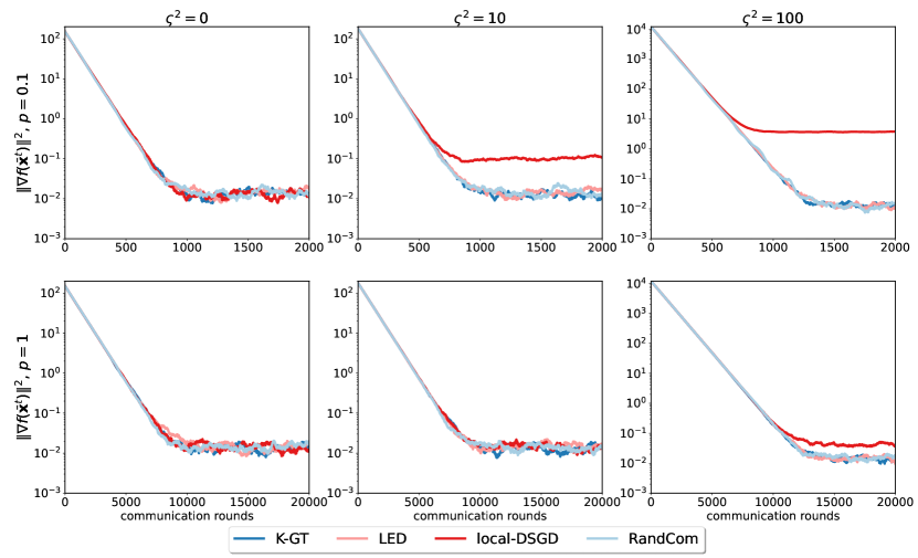
Figure 1: Learning SYNTHETIC convex function over $10$ nodes with noise $\sigma^{2}=1$ (Local-DSGD [16, 9], $K$-GT [18], and LED [19]). All uses the same learning rate and are averaged by ten repetitions. The probability of communication for RandCom is $p$, and the number of local updates of local-DSGD, $K$-GT, and LED are $\nicefrac{{1}}{{p}}$.

4.2 Real-world Dataset ijcnn1

In this subsection, we use numerical experiments to demonstrate our findings on the logistic regression problem with a regularizer. The objective function is defined as follows:

$$f({\bf{x}})=\frac{1}{n}\sum_{i=1}^{n}\big{\{}\frac{1}{m_{i}}\sum_{j=1}^{m_{i}}\ln(1+e^{-(\mathcal{A}_{ij}^{\sf T}{{\bf{x}}})\mathcal{B}_{ij}})\big{\}}+r({\bf{x}}).$$

Here, $r({\bf{x}})$ is the regularizer, any node $i$ holds its own training date $\left(\mathcal{A}_{ij},\mathcal{B}_{ij}\right)\in$ $\mathbb{R}^{d}\times\{-1,1\},j=1,\cdots,m_{i}$, including sample vectors $\mathcal{A}_{ij}$ and corresponding classes $\mathcal{B}_{ij}$. We use the dataset ijcnn1 [37], whose attributes is $d=22$ and $\sum_{i=1}^{n}m_{i}=49950$. Moreover, the training samples are randomly and evenly distributed over all the $n$ agents. We control the stochastic noise $\sigma^{2}$ by adding Gaussian noise to every stochastic gradient, i.e., the stochastic gradients are generated as follows: $\nabla F_{i}({\bf{x}})=\nabla f_{i}({\bf{x}})+\omega_{i}$, where $\omega_{i}\thicksim\mathcal{N}(0,\sigma^{2}{\bf{I}}_{d})$ and $\sigma=10^{-3}$.

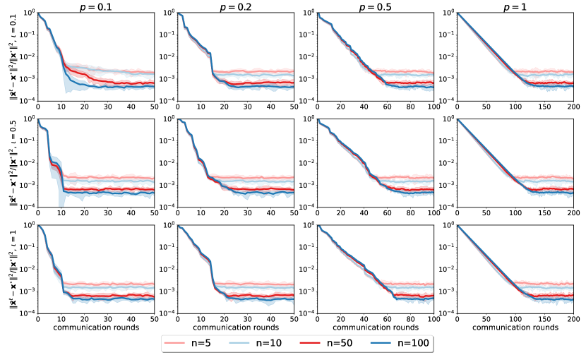
Figure 2: Experimental results for RandCom to logistic regression problem with a strongly convex regularizer $r({\bf{x}})=\frac{1}{2}\|{\bf{x}}\|^{2}$ over ijcnn1 dataset.

Convex Regularizer: We choose the regularizer $r({\bf{x}})=\frac{1}{2}\|{\bf{x}}\|^{2}$ to demonstrate the results in stochastic strongly convex setting. The results are shown in Fig. 2. The relative error $\nicefrac{{\|\bar{{\bf{x}}}^{t}-{\bf{x}}^{\star}\|^{2}}}{{\|{\bf{x}}^{\star}\|^{2}}}$ is shown on the $y$-axis. Here, we set $\alpha=\nicefrac{{1}}{{2L}}$, which independent of the network topology, and set $\chi=\mathcal{O}(\nicefrac{{1}}{{p}})$ and $\beta=p$. We show the performance of RandCom at different network connectivity $\iota$ and communication probability $p$. The results show that, when the number of nodes is increased, the relative errors of RandCom is reduced under a constant and network-independent stepsize, which validates our results about linear speedup under strongly convexity. Note that, when $\iota=1$, the network is fully connected and the global mixing matrix ${\bf{W}}=\nicefrac{{1}}{{n}}{\bf{11}}^{\sf T}$. In this case, we also show the performance of Algorithm 2.

Non-convex Regularizer: We choose the regularizer $r({\bf{x}})=\sum_{j=1}^{d}\frac{{\bf{x}}(j)^{2}}{1+{\bf{x}}(j)^{2}}$ and $n=10$ to demonstrate the results in stochastic non-convex setting, where ${\bf{x}}=\mathrm{col}\{{\bf{x}}(j)\}_{j=1}^{d}\in\mathbb{R}^{d}$. In this case, Fig. 3 compares RandCom to the decentralized methods Local-DSGD [16, 9], $K$-GT [18], and LED [19] for different local steps $\nicefrac{{1}}{{p}}=10,5,1$. We use the same stepsize $\alpha=0.01$ for all algorithms. For RandCom, we set $\beta=1$ and $\chi=\mathcal{O}(\nicefrac{{1}}{{p}})$. When $\iota=0.1$, we know that RandCom and LED perform similarly, and they outperforms the other methods as we increase the number of local steps. When $\iota=1$, we observe that RandCom, $K$-GT [18], and LED [19] perform similarly, and Local-DSGD [16, 9] (when $\iota=1$, it is equivalent to Local-SGD/FedAvg) performance degrades as the number of local updates increases, as expected. Furthermore, it is worth noting that increasing the number of local steps reduces the amount of communication required to achieve the same level of accuracy.

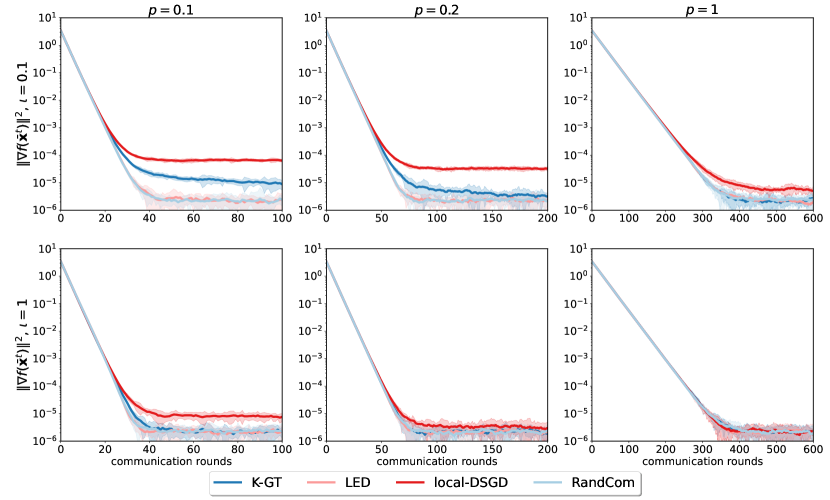
Figure 3: Experimental results for RandCom to logistic regression problem with a non-convex regularizer $r({\bf{x}})=\sum_{j=1}^{d}\frac{{\bf{x}}(j)^{2}}{1+{\bf{x}}(j)^{2}}$ over ijcnn1 dataset (Local-DSGD [16, 9], $K$-GT [18], and LED [19]).

5 Conclusion

In this paper, we introduced RandCom, an optimization method for stochastic decentralized optimization problems, which incorporates probabilistic local updates. We investigated the performance of RandCom in stochastic non-convex, convex and strongly convex settings. The results indicated that its rates are comparable to the best existing decentralized and centralized bounds and it can achieve linear speedup by the number of nodes $n$ and the communication probability $p$. We further demonstrated its ability to achieve linear speedup with network-independent stepsizes for stochastic strongly convex settings. Additionally, we extended the theoretical findings to the domain of federated learning.

However, there are still open and challenging questions in the decentralized setting that warrant further exploration. One such question pertains to the compatibility of probabilistic local updates with partial participation [14], a desirable feature that allows only a subset of nodes to participate in each round of the training process. Investigating the potential combination of probabilistic local updates with communication compression [15] represents another intriguing direction for future research. We consider these aspects as important avenues for future work.

Appendix

Appendix A Preliminaries

In this section, we prove Theorem 1. We will first introduce some basic facts and notations, then using the analysis tool provided by [36], we give two equivalent transformations of RandCom. Based on these two transformations, we establish the convergence analysis.

A.1 Basic Facts

The stochastic processes such as randomized communication and gradient estimation generate two sequences of $\sigma$-algebra. We denote by $\mathcal{G}^{t}$ the $\sigma$-algebra of gradient estimation at $t$-th iteration and $\mathcal{F}^{t}$ the $\sigma$-algebra of randomized communication at the same step. The sequences $\{\mathcal{G}^{t}\}_{t\geq 0}$ and $\{\mathcal{F}^{t}\}_{t\geq 0}$ satisfy

$$\mathcal{G}^{0}\subset\mathcal{F}^{0}\subset\mathcal{G}^{1}\subset\mathcal{F}^{1}\subset\mathcal{G}^{2}\subset\mathcal{F}^{2}\subset\cdots\subset\mathcal{G}^{t}\subset\mathcal{F}^{t}\subset\cdots\ .$$

With these notations, we can clarify the stochastic dependencies among the variables generated by RandCom (Algorithmd 1 or 2), i.e., $({\bf{G}}^{t},\hat{{\bf{Z}}}^{t})$ is measurable in $\mathcal{G}^{t}$ and $({\bf{Y}}^{t+1},{\bf{X}}^{t+1})$ is measurable in $\mathcal{F}^{t}$.

The Bregman divergence of $f$ at points $(x,y)$ is defined by

$$D_{f}(x,y):=f(x)-f(y)-\langle\nabla f(y),x-y\rangle.$$

It is easy to verify that $\langle\nabla f(x)-\nabla f(y),x-y\rangle=D_{f}(x,y)+D_{f}(y,x)$. If $f$ is convex, from the definition of convex function, we have $D_{f}(x,y)\geq 0$ and $D_{f}(y,x)\geq 0$. Thus

$$\langle\nabla f(x)-\nabla f(y),x-y\rangle\geq D_{f}(x,y),\text{ and }\langle\nabla f(x)-\nabla f(y),x-y\rangle\geq D_{f}(y,x).$$ (18)

For an $L$-smooth and $\mu$-strongly convex function $f$, by [13, Appendix. A] we have

$$\frac{\mu}{2}\|x-y\|^{2}\leq D_{f}(x,y)\leq\frac{L}{2}\|x-y\|^{2},$$ (19)

$$\frac{1}{2L}\|\nabla f(x)-\nabla f(y)\|^{2}\leq D_{f}(x,y)\leq\frac{1}{2\mu}\|\nabla f(x)-\nabla f(y)\|^{2}.$$ (20)

A.2 Notations

For any $n\times m$ matrices $\mathbf{a}$ and $\mathbf{b}$, their inner product is denoted as $\langle\mathbf{a},\mathbf{b}\rangle=\mathrm{Trace}(\mathbf{a}^{\sf T}\mathbf{b})$. For a given matrix $\mathbf{a}$, the Frobenius norm is given by $\|\mathbf{a}\|_{\mathrm{F}}$, while the spectral norm is given by $\|\mathbf{a}\|$. Define the gradient and communication noise as

$${\bf{S}}^{t}=[{\bf{s}}^{t}_{1},\ldots,{\bf{s}}^{t}_{n}]^{\sf T}={\bf{G}}^{t}-\nabla F({\bf{X}}^{t}),\text{ where }{\bf{s}}^{t}_{i}={\bf{g}}_{i}^{t}-\nabla f_{i}({\bf{x}}_{i}^{t});\quad{\bf{E}}^{t}=\frac{1}{2\chi}(\theta_{t}-1){\bf{W}}_{b}\hat{{\bf{Z}}}^{t}.$$

We also define the following notations to simplify the analysis:

$$\bar{{\bf{x}}}^{t}\triangleq\big{(}\frac{1}{n}\sum_{i=1}^{n}{\bf{x}}_{i}^{t}\big{)}^{\sf T},\quad\bar{{\bf{X}}}^{t}={\bf{1}}\otimes\bar{{\bf{x}}}^{t},\quad\bar{{\bf{s}}}^{t}\triangleq\big{(}\frac{1}{n}\sum_{i=1}^{n}{\bf{s}}_{i}^{t}\big{)}^{\sf T},\quad\overline{\nabla F}({\bf{X}}^{t})\triangleq\big{(}\frac{1}{n}\sum_{i=1}^{n}\nabla f_{i}({\bf{x}}^{t}_{i})\big{)}^{\sf T}.$$

With Assumption 1, the mixing matrix ${\bf{W}}$ can be decomposed as

$${\bf{W}}={\bf{P\Lambda P}}^{-1}=\left[\begin{array}[]{cc}{\bf{1}}&\hat{{\bf{P}}}\\ \end{array}\right]\left[\begin{array}[]{cc}{\bf{I}}&0\\ 0&\hat{{\bf{\Lambda}}}\\ \end{array}\right]\left[\begin{array}[]{c}\frac{1}{n}{\bf{1}}^{\sf T}\\ \hat{{\bf{P}}}^{\sf T}\\ \end{array}\right]$$

where $\hat{{\bf{\Lambda}}}=\mathrm{diag}\{\lambda_{2},\ldots,\lambda_{n}\}$, and matrix $\hat{{\bf{P}}}\in\mathbb{R}^{n\times(n-1)}$ satisfies

$$\hat{{\bf{P}}}^{\sf T}\hat{{\bf{P}}}={\bf{I}},\ {\bf{1}}^{\sf T}\hat{{\bf{P}}}=0,\ \hat{{\bf{P}}}\hat{{\bf{P}}}^{\sf T}={\bf{I}}-\frac{1}{n}{\bf{11}}^{\sf T}.$$

Therefore, it holds that

$${\bf{W}}_{a}=\left[\begin{array}[]{cc}{\bf{1}}&\hat{{\bf{P}}}\\ \end{array}\right]\underbrace{\left[\begin{array}[]{cc}{\bf{1}}&0\\ 0&\hat{{\bf{\Lambda}}}_{a}\\ \end{array}\right]}_{:={\bf{\Lambda}}_{a}}\left[\begin{array}[]{c}\frac{1}{n}{\bf{1}}^{\sf T}\\ \hat{{\bf{P}}}^{\sf T}\\ \end{array}\right],~{}{\bf{W}}_{b}^{2}=\left[\begin{array}[]{cc}{\bf{1}}&\hat{{\bf{P}}}\\ \end{array}\right]\underbrace{\left[\begin{array}[]{cc}0&0\\ 0&\hat{{\bf{\Lambda}}}_{b}^{2}\\ \end{array}\right]}_{:={\bf{\Lambda}}_{b}^{2}}\left[\begin{array}[]{c}\frac{1}{n}{\bf{1}}^{\sf T}\\ \hat{{\bf{P}}}^{\sf T}\\ \end{array}\right],$$ (31)

where $\hat{{\bf{\Lambda}}}_{a}={\bf{I}}-\frac{1}{2\chi}({\bf{I}}-\hat{{\bf{\Lambda}}})$, $\hat{{\bf{\Lambda}}}_{b}=\sqrt{{\bf{I}}-\hat{{\bf{\Lambda}}}}$. Since $\lambda_{i}\in(-1,1)$ for $i=2,\dots,n$, it holds that $1-\frac{1}{2\chi}(1-\lambda_{i})\in[0,1)$ and $0\preceq{\bf{W}}_{a}\prec{\bf{I}}$ for $\chi\geq 1$.

A.3 Transformation and Some Descent Inequalities

Here, we introduce an auxiliary variable ${\bf{R}}^{t}={\bf{Y}}^{t}+\alpha\nabla F(\bar{{\bf{X}}}^{t})$, where $\bar{{\bf{X}}}^{t}=\mathbf{1}\otimes\bar{{\bf{x}}}^{t}$. It follows from (3b) and (3c) that, when $\beta=1$ and $p=1$, ${\bf{Y}}^{t+1}={\bf{Y}}^{t}+\frac{1}{2\chi}{\bf{W}}_{b}^{2}\hat{{\bf{Z}}}^{t}$. For any fixed point $({\bf{X}},{\bf{Y}})$ of RandCom (3), it holds that $\hat{{\bf{Z}}}={\bf{X}}$, ${\bf{Y}}+\alpha\nabla F({{\bf{X}}})=0$, ${\bf{W}}_{b}{\bf{X}}=0$. Thus, ${\bf{R}}=0$ implies that $\frac{1}{n}\sum_{i=1}^{n}\nabla f_{i}({\bf{x}})=0$, i.e., ${\bf{x}}$ is a stationary point of problem (1). By this new variable, we give following error dynamics of RandCom.

Lemma 1 (Error Dynamics of RandCom).

Suppose Assumption 1 holds. If $\beta=1$, there exist a invertible matrix ${\bf{Q}}$ and a diagonal matrix ${\bf{\Gamma}}$ such that

$$\bar{{\bf{x}}}^{t+1} =\bar{{\bf{x}}}^{t}-\alpha\overline{\nabla F}({\bf{X}}^{t})-\alpha\bar{{\bf{s}}}^{t},$$ (32a)

$$\mathcal{E}^{t+1} =\underbrace{{\bf{\Gamma}}\mathcal{E}^{t}-\alpha\upsilon{\bf{Q}}^{-1}\left[\begin{array}[]{c}\hat{{\bf{\Lambda}}}_{a}\hat{{\bf{P}}}^{\sf T}{\bf{\Sigma}}_{1}^{t}\\ \frac{1}{2\chi}\hat{{\bf{\Lambda}}}_{b}^{2}\hat{{\bf{P}}}^{\sf T}{\bf{\Sigma}}_{1}^{t}+\hat{{\bf{P}}}^{\sf T}{\bf{\Sigma}}_{2}^{t}\\ \end{array}\right]}_{:=\mathbb{G}^{t}}+\underbrace{\upsilon{\bf{Q}}^{-1}\left[\begin{array}[]{c}-\hat{{\bf{\Lambda}}}_{b}\hat{{\bf{P}}}^{\sf T}{\bf{E}}^{t}\\ \hat{{\bf{\Lambda}}}_{b}\hat{{\bf{P}}}^{\sf T}{\bf{E}}^{t}\\ \end{array}\right]}_{:=\mathbb{F}^{t}},$$ (32f)

where $\upsilon>0$, ${\bf{\Sigma}}_{1}^{t}=\nabla F({\bf{X}}^{t})-\nabla F(\bar{{\bf{X}}}^{t})+{\bf{S}}^{t}$, ${\bf{\Sigma}}_{2}^{t}=\nabla F(\bar{{\bf{X}}}^{t})-\nabla F(\bar{{\bf{X}}}^{t+1})$,

$$\mathcal{E}^{t}\triangleq\upsilon{\bf{Q}}^{-1}\left[\begin{array}[]{c}\hat{{\bf{P}}}^{\sf T}{{\bf{X}}}^{t}\\ \hat{{\bf{P}}}^{\sf T}{{\bf{R}}}^{t}\\ \end{array}\right],\text{ and }\gamma\triangleq\|{\bf{\Gamma}}\|=\sqrt{1-\frac{1}{2\chi}(1-\lambda_{2})}<1.$$

Moreover, we have

$$\|{\bf{Q}}\|^{2}\leq 2\text{ and }\|{\bf{Q}}^{-1}\|^{2}\leq\frac{2\chi}{(1+\lambda_{n})(1-\lambda_{2})}.$$

Proof.

See Appendix E. ∎

Based on Lemma 1, and inspired by [16, Lemma 8] and [36, Lemma 3 and Lemma 4], we give the following descent inequalities.

Lemma 2.

Suppose Assumptions 1, 2, and 3 hold. Let $\upsilon=1$. If $\alpha\leq\frac{1}{2L}$ and $\beta=1$, it holds that

$$\mathbb{E}\!\left[f(\bar{{\bf{x}}}^{t+1})\;|\;\mathcal{G}^{t}\right]\leq f(\bar{{\bf{x}}}^{t})-\frac{\alpha}{2}\big{\|}\nabla f(\bar{{\bf{x}}}^{t})\big{\|}^{2}+\frac{2\alpha L^{2}}{n}\big{\|}\mathcal{E}^{t}\big{\|}_{\mathrm{F}}^{2}+\frac{L\alpha^{2}\sigma^{2}}{2n},$$ (33)

$$\mathbb{E}\!\left[\|\mathcal{E}^{t+1}\|_{\mathrm{F}}^{2}\;|\;\mathcal{G}^{t}\right]\leq \tilde{\gamma}\|\mathcal{E}^{t}\|_{\mathrm{F}}^{2}+\frac{4n\alpha^{4}L^{2}\|({\bf{I}}-\hat{{\bf{\Lambda}}}_{a})^{-1}\|}{1-\gamma}\|\nabla f(\bar{{\bf{x}}}^{t})\|^{2}$$

$$+\frac{2\alpha^{4}L^{2}\sigma^{2}\|({\bf{I}}-\hat{{\bf{\Lambda}}}_{a})^{-1}\|}{1-\gamma}+\frac{2n\alpha^{2}\sigma^{2}(2\chi^{2}+(1-p))}{\chi^{2}},$$ (34)

where

$$\tilde{\gamma}=\gamma+\frac{32\alpha^{2}L^{2}+16\alpha^{4}L^{4}\|({\bf{I}}-\hat{{\bf{\Lambda}}}_{a})^{-1}\|}{1-\gamma}+\frac{2(1-p)\big{(}3+\frac{24\chi\alpha^{2}L^{2}}{(1+\lambda_{n})(1-\lambda_{2})}\big{)}}{\chi^{2}}.$$ (35)

Moreover, if $f_{i}$ is $\mu$-convex ($\mu\geq 0$) and $\alpha\leq\frac{1}{4L}$, it holds that

$$\mathbb{E}\!\left[\big{\|}\bar{{\bf{x}}}^{t+1}-{\bf{x}}^{\star}\big{\|}^{2}\;|\;\mathcal{G}^{t}\right]\leq(1-\mu\alpha)\|\bar{{\bf{x}}}^{t}-{\bf{x}}^{\star}\|^{2}+\frac{6\alpha L}{n}\|\mathcal{E}^{t}\|_{\mathrm{F}}^{2}+\frac{\alpha^{2}\sigma^{2}}{n}-\alpha(f(\bar{{\bf{x}}}^{t})-f({\bf{x}}^{\star})),$$ (36)

where ${\bf{x}}^{\star}$ solves problem (1).

Proof.

See Appendix F. ∎

Appendix B Convergence Analysis: Non-convex

With Lemma 1 and Lemma 2, we further have the following lemma.

Lemma 3 (Non-Convex Setting).

Suppose Assumptions 1, 2, and 3 hold. If $\beta=1$, $p\in[\nicefrac{{1}}{{\chi}},1]$, $\alpha$ and $\chi$ satisfy that $\chi\geq\max\left\{\frac{288(1-p)}{1-\lambda_{2}},1\right\}$

$$0<\alpha\leq\min\left\{\frac{1}{2L},\frac{1-\lambda_{2}}{32\sqrt{3}\chi L},\sqrt{\frac{(1+\lambda_{n})(1-\lambda_{2})}{2\chi}}\frac{1}{2L},\sqrt[4]{\frac{(1-\lambda_{2})^{3}}{12\chi^{3}}}\frac{1}{4L}\right\},$$ (37)

it holds that $\tilde{\gamma}\leq\frac{1+\gamma}{2}<1$ and

$$\frac{1}{T}\sum_{t=0}^{T-1}\mathbb{E}\!\left[\big{\|}\nabla f(\bar{{\bf{x}}}^{t})\big{\|}^{2}\right]\leq \frac{4(f(\bar{{\bf{x}}}^{0})-f^{*})}{\alpha T}+\frac{128\chi^{2}L^{2}\alpha^{2}\varsigma^{2}_{0}}{(1-\lambda_{2})^{2}T}+\frac{2L\alpha\sigma^{2}}{n}$$

$$+\frac{\alpha^{2}L^{2}\sigma^{2}\big{(}\chi^{3}+256\chi(2\chi^{2}+(1-p))\big{)}}{2(1-\lambda_{2})\chi^{2}},$$ (38)

where $\varsigma^{2}_{0}=\frac{1}{n}\sum_{i=1}^{n}\|\nabla f_{i}(\bar{{\bf{x}}}^{0})-\nabla f(\bar{{\bf{x}}}^{0})\|^{2}$.

Proof.

See Appendix G. ∎

We can even get a tighter rate by carefully selecting the step size similar to [10], [16], [18] and [19]. From the condition of stepsize, we have $\alpha=\mathcal{O}(\nicefrac{{(1-\lambda_{2})}}{{\chi L}})$. Then, we can prove that there exist a constant $\alpha=\mathcal{O}(\nicefrac{{(1-\lambda_{2})}}{{\chi L}})$ such that

$$\frac{1}{T}\sum_{t=0}^{T-1}\mathbb{E}[\|\nabla f(\bar{{\bf{x}}}^{t})\|^{2}]\leq\mathcal{O}\left(\sqrt{\frac{L(f(\bar{{\bf{x}}}^{0})-f^{\star})\sigma^{2}}{nT}}\right)$$

$$+\mathcal{O}\left(\sqrt[3]{\frac{\chi^{3}+\chi(1-p)}{(1-\lambda_{2})\chi^{2}}}(\frac{L(f(\bar{{\bf{x}}}^{0})-f^{\star})\sigma}{T})^{\frac{2}{3}}\right)+\mathcal{O}\left(\frac{\frac{\chi L(f(\bar{{\bf{x}}}^{0})-f^{\star})}{(1-\lambda_{2})}+\varsigma_{0}^{2}}{T}\right).$$

Here, we omit the proof, as this proof is standard, and it can be easily derived from [16, Lemma 17], [18, Lemma C.13], or [19, Corollary 1]. Then, it follows that

$$\frac{1}{T}\sum_{t=0}^{T-1}\mathbb{E}[\|\nabla f(\bar{{\bf{x}}}^{t})\|^{2}]\leq\mathcal{O}\left(\left(\frac{L\sigma^{2}}{nT}\right)^{\frac{1}{2}}+\left(\frac{\chi L^{2}\sigma^{2}}{(1-\lambda_{2})T^{2}}\right)^{\frac{1}{3}}+\frac{L\chi}{(1-\lambda_{2})T}\right).$$

When $p<\lambda_{2}$, we have $\max\left\{\nicefrac{{288(1-p)}}{{1-\lambda_{2}}},1\right\}=\mathcal{O}(\nicefrac{{1}}{{(1-\lambda_{2})}})$. Choosing $\chi=\max\left\{\nicefrac{{288(1-p)}}{{1-\lambda_{2}}},1\right\}$. Since in each iteration we trigger communication with probability $p$, for any desired accuracy $\epsilon>0$, the expected number of communication rounds required to achieve $\frac{1}{T}\sum_{t=0}^{T-1}\mathbb{E}[\|\nabla f(\bar{{\bf{x}}}^{t})\|^{2}]\leq\epsilon$ is bounded by $p\times\text{(iteration complexity)}$:

$$\mathcal{O}\left(\frac{p\sigma^{2}L}{n\epsilon^{2}}+\frac{p}{1-\lambda_{2}}\frac{\sigma L}{\epsilon^{\nicefrac{{3}}{{2}}}}+\frac{p}{(1-\lambda_{2})^{2}}\frac{L}{\epsilon}\right).$$

When $p\geq\lambda_{2}$, we have $\max\left\{\nicefrac{{288(1-p)}}{{1-\lambda_{2}}},1\right\}=\mathcal{O}(1)$. If we choose $\chi$ such that $\chi=\max\left\{\nicefrac{{288(1-p)}}{{1-\lambda_{2}}},1\right\}$, then for any desired accuracy $\epsilon>0$, the expected communication complexity of RandCom is bounded by

$$\mathcal{O}\left(\frac{p\sigma^{2}L}{n\epsilon^{2}}+\frac{p}{\sqrt{1-\lambda_{2}}}\frac{\sigma L}{\epsilon^{\nicefrac{{3}}{{2}}}}+\frac{p}{(1-\lambda_{2})}\frac{L}{\epsilon}\right).$$

Therefore, the expected communication complexity (8) in non-convex settings holds.

Appendix C Convergence Analysis: Convex

By Lemma 1 and Lemma 2, we also can deduce the following lemma.

Lemma 4 (Convex Setting).

Suppose Assumptions 1, 2, and 3 hold. If $\beta=1$, $p\in[\nicefrac{{1}}{{\chi}},1]$, $\alpha$ and $\chi$ satisfy that $\chi\geq\max\left\{\frac{288(1-p)}{1-\lambda_{2}},1\right\}$

$$0<\alpha\leq\min\left\{\frac{1}{2L},\frac{1-\lambda_{2}}{32\sqrt{3}\chi L},\sqrt{\frac{(1+\lambda_{n})(1-\lambda_{2})}{2\chi}}\frac{1}{2L},\sqrt[4]{\frac{(1-\lambda_{2})^{3}}{24\chi^{3}}}\frac{1}{4L}\right\},$$ (39)

it holds that

$$\frac{1}{T}\sum_{t=0}^{T-1}\mathbb{E}\!\left[f(\bar{{\bf{x}}}^{t})-f^{\star}\right]\leq \frac{2\|\bar{{\bf{x}}}^{0}-{\bf{x}}^{\star}\|^{2}}{\alpha T}+\frac{192\chi^{2}\alpha^{2}L\varsigma^{2}_{0}}{(1-\lambda_{2})^{2}T}+\frac{2\alpha\sigma^{2}}{n}+\frac{L\alpha^{2}\sigma^{2}\big{(}\chi^{3}+384\chi(2\chi^{2}+(1-p))\big{)}}{2(1-\lambda_{2})\chi^{2}}.$$ (40)

Proof.

See Appendix H. ∎

Similar as the analysis of non-convex setting, with Lemma 4, we have there exist a constant $\alpha=\mathcal{O}(\nicefrac{{1-\lambda_{2}}}{{\chi L}})$ such that

$$\frac{1}{T}\sum_{t=0}^{T-1}\mathbb{E}\!\left[f(\bar{{\bf{x}}}^{t})-f^{\star}\right]\leq\mathcal{O}\left(\sqrt{\frac{\sigma^{2}}{nT}}+\sqrt[3]{\frac{\chi^{2}+(1-p)}{(1-\lambda_{2})\chi}}(\frac{\sqrt{L}\sigma}{T})^{\frac{2}{3}}+\frac{L\chi}{(1-\lambda_{2})T}\right).$$

When $p<\lambda_{2}$ and choosing $\chi=\max\left\{\nicefrac{{288(1-p)}}{{1-\lambda_{2}}},1\right\}\leq\mathcal{O}(\nicefrac{{1}}{{(1-\lambda_{2})}})$, for any desired accuracy $\epsilon>0$, the expected communication complexity of RandCom is bounded by

$$\mathcal{O}\left(\frac{p\sigma^{2}}{n\epsilon^{2}}+\frac{p}{(1-\lambda_{2})}\frac{\sigma\sqrt{L}}{\epsilon^{\nicefrac{{3}}{{2}}}}+\frac{p}{(1-\lambda_{2})^{2}}\frac{L}{\epsilon}\right).$$

When $p\geq\lambda_{2}$, we have $\max\left\{\nicefrac{{288(1-p)}}{{1-\lambda_{2}}},1\right\}=\mathcal{O}(1)$. If we choose $\chi$ such that $\chi=\max\left\{\nicefrac{{288(1-p)}}{{1-\lambda_{2}}},1\right\}$, then for any desired accuracy $\epsilon>0$, the expected communication complexity of RandCom is bounded by

$$\mathcal{O}\left(\frac{p\sigma^{2}}{n\epsilon^{2}}+\frac{p}{\sqrt{1-\lambda_{2}}}\frac{\sigma\sqrt{L}}{\epsilon^{\nicefrac{{3}}{{2}}}}+\frac{p}{1-\lambda_{2}}\frac{L}{\epsilon}\right).$$

Thus, the expected communication complexity (11) of RandCom in convex settings follows.

Appendix D Convergence Analysis: Strongly Convex

By Lemma 1 and Lemma 2, we also can deduce the following lemma.

Lemma 5 (Strongly Convex Setting).

Suppose Assumptions 1, 2, and 3 hold. If $\beta=1$, $p\in[\nicefrac{{1}}{{\chi}},1]$, $\alpha$ and $\chi$ satisfy that $\chi\geq\max\left\{\frac{288(1-p)}{1-\lambda_{2}},1\right\}$ and

$$0<\alpha\leq\min\left\{\frac{1}{2L},\frac{1-\lambda_{2}}{32\sqrt{3}\chi L},\sqrt{\frac{(1+\lambda_{n})(1-\lambda_{2})}{2\chi}}\frac{1}{2L},\frac{72\mu}{L^{2}},\frac{1-\gamma}{12L+\nicefrac{{\mu}}{{2}}},\sqrt[3]{4\mu(1-\gamma)}\frac{1}{L}\right\},$$ (41)

it holds that

$$\mathbb{E}\!\left[\big{\|}\bar{{\bf{x}}}^{t}-{\bf{x}}^{\star}\big{\|}^{2}\right]\leq \Big{(}1-\frac{\alpha\mu}{4}\Big{)}^{t}\Big{(}\big{\|}\bar{{\bf{x}}}^{0}-{\bf{x}}^{\star}\big{\|}^{2}+\frac{4\chi\alpha^{2}\varsigma_{0}^{2}}{1-\lambda_{2}}\Big{)}$$

$$+\frac{2\alpha\sigma^{2}}{\mu n}+\frac{7L\alpha^{2}\sigma^{2}(192\chi^{2}+(4\chi^{2}+2(1-p)))}{12\mu(1-\lambda_{2})\chi}.$$ (42)

Proof.

See Appendix I. ∎

From condition of the stepsize $\alpha$, we have $\alpha=\mathcal{O}(\nicefrac{{\mu(1-\lambda_{2})}}{{\chi L^{2}}})$. Similar as [19, Corollary 1], we can show that there exist a constant $\alpha$ such that

$$\mathbb{E}[\|\bar{{\bf{x}}}^{T}-{\bf{x}}^{\star}\|^{2}]\leq\tilde{\mathcal{O}}\left(\frac{\sigma^{2}}{nT}+\frac{\sigma^{2}(\chi^{2}+(1-p))}{(1-\lambda_{2})\chi T^{2}}+\mathrm{exp}[-\frac{(1-\lambda_{2})T}{\chi}]a_{0}\right),$$

where $a_{0}$ is a constant that depends on the initialization. Similar as the analysis of non-convex and convex settings, we have $\chi=\max\{\nicefrac{{288(1-p)}}{{1-\lambda_{2}}},1\}\leq\mathcal{O}(\nicefrac{{1}}{{(1-\lambda_{2})}})$ if $p<\lambda_{2}$ and $\chi=\max\{\nicefrac{{288(1-p)}}{{1-\lambda_{2}}},1\}=\mathcal{O}(1)$ if $p\geq\lambda_{2}$. Thus, for any desired accuracy $\epsilon>0$, the expected number of communication rounds required to achieve $\mu\mathbb{E}[\|\bar{{\bf{x}}}^{T}-{\bf{x}}^{\star}\|^{2}]\leq\epsilon$ is bounded by

$$\tilde{\mathcal{O}}\left(\frac{p\sigma^{2}}{n\mu\epsilon}+\frac{p}{{1-\lambda_{2}}}\frac{\sigma\sqrt{L}}{\mu\sqrt{\epsilon}}+\frac{p\kappa^{2}\mathrm{log}\nicefrac{{1}}{{\epsilon}}}{(1-\lambda_{2})^{2}}\right),\ p\in(0,\lambda_{2}),$$

and

$$\tilde{\mathcal{O}}\left(\frac{p\sigma^{2}}{n\mu\epsilon}+\frac{p}{\sqrt{1-\lambda_{2}}}\frac{\sigma\sqrt{L}}{\mu\sqrt{\epsilon}}+\frac{p\kappa^{2}\mathrm{log}\nicefrac{{1}}{{\epsilon}}}{1-\lambda_{2}}\right),\ p\in[\lambda_{2},1],$$

i.e., the expected communication complexity (14) holds.

Then, we further prove RandCom can achieve linear speedup with network-independent stepsize. We introduce new iterates $\{{\bf{U}}^{t}\}$ to facilitate the analysis. Similar techniques can be found, e.g., in [29, 30, 31, 32], ${\bf{Y}}^{t}=\alpha{\bf{W}}_{b}{\bf{U}}^{t}$. Since ${\bf{I}}-{\bf{W}}_{a}=\frac{1}{2\chi}{\bf{W}}^{2}_{b}$, from (3b) and (3c), we have

$$\left\{\begin{array}[]{rl}{\bf{X}}^{t+1}\ =&(1-\theta_{t})\hat{{\bf{Z}}}^{t}+\theta_{t}{\bf{W}}_{a}\hat{{\bf{Z}}}^{t}\\ \alpha{\bf{W}}_{b}{\bf{U}}^{t+1}\ =&\alpha{\bf{W}}_{b}{\bf{U}}^{t}+\beta(\hat{{\bf{Z}}}^{t}-{\bf{X}}^{t+1})\end{array}\right.\Longleftrightarrow\left\{\begin{array}[]{rl}{\bf{W}}_{b}{\bf{U}}^{t+1}\ =&{\bf{W}}_{b}{\bf{U}}^{t}+\frac{\beta\theta_{t}}{2\chi\alpha}{\bf{W}}_{b}^{2}\hat{{\bf{Z}}}^{t}\\ {\bf{X}}^{t+1}\ =&\hat{{\bf{Z}}}^{t}-\frac{\alpha}{\beta}{\bf{W}}_{b}({\bf{U}}^{t+1}-{\bf{U}}^{t})\end{array}\right..$$

Therefore, letting ${\bf{Y}}^{0}=0$, we have the following equivalent form of RandCom (3) in the sense that they generate an identical sequence $({\bf{X}}^{t},\hat{{\bf{Z}}}^{t})$.

$$\hat{{\bf{Z}}}^{t} =\ {\bf{X}}^{t}-\alpha{\bf{G}}^{t}-\alpha{\bf{W}}_{b}{\bf{U}}^{t},$$ (43a)

$${\bf{U}}^{t+1} =\ {\bf{U}}^{t}+\frac{\beta\theta_{t}}{2\chi\alpha}{\bf{W}}_{b}\hat{{\bf{Z}}}^{t},$$ (43b)

$${\bf{X}}^{t+1} =\ \hat{{\bf{Z}}}^{t}-\frac{\alpha}{\beta}{\bf{W}}_{b}({\bf{U}}^{t+1}-{\bf{U}}^{t}).$$ (43c)

This equivalent form is more useful for the subsequent convergence analysis. The optimality condition of problem (2) is as the following lemma.

Lemma 6.

Suppose Assumption 1 holds. If there exists a point $({\bf{X}}^{\star},{\bf{U}}^{\star})$ that satisfies:

$$0 =\nabla F({\bf{X}}^{\star})+{\bf{W}}_{b}{\bf{U}}^{\star},$$ (44a)

$$0 ={\bf{W}}_{b}{\bf{Z}}^{\star},$$ (44b)

then it holds that ${\bf{X}}^{\star}=[{\bf{x}}^{\star},{\bf{x}}^{\star},\ldots,{\bf{x}}^{\star}]^{\sf T}$, where ${\bf{x}}^{\star}\in\mathbb{R}^{d}$ is a stationary point to problem (1).

From Lemma 6, when ${\bf{G}}^{t}=\nabla F({\bf{X}}^{t})$, we have that any fixed point of (43) satisfies the condition (44). We also define the following notations to simplify the analysis:

$$\widetilde{{\bf{Z}}}^{t}\triangleq\hat{{\bf{Z}}}^{t}-{\bf{X}}^{\star},\quad\widetilde{{\bf{X}}}^{t}\triangleq{\bf{X}}^{t}-{\bf{X}}^{\star},\quad\widetilde{{\bf{U}}}^{t}\triangleq\alpha({\bf{U}}^{t}-{\bf{U}}^{\star}),\quad\bar{{\bf{e}}}^{t}\triangleq\bar{{\bf{x}}}^{t}-({\bf{x}}^{\star})^{\sf T},$$

where $({\bf{X}}^{\star},{\bf{U}}^{\star})$ satisfies (44). Similar as Lemma 1, we give another error dynamics of RandCom, which will be used for proving the linear speedup with network-independent stepsizes of RandCom under strongly convexity.

Lemma 7 (Another Error Dynamics of RandCom).

Suppose Assumption 1 holds. If $\beta=p$ and $p\in[\nicefrac{{1}}{{\chi}},1]$, there exist a invertible matrix ${\bf{Q}}^{\mathrm{s}}$ and a diagonal matrix ${\bf{\Gamma}}$ such that

$$\bar{{\bf{e}}}^{t+1} =\bar{{\bf{e}}}^{t}-\alpha\overline{\nabla F}({\bf{X}}^{t})-\alpha\bar{{\bf{s}}}^{k},$$ (45a)

$$\mathcal{E}_{\mathrm{s}}^{t+1} =\underbrace{{\bf{\Gamma}}\mathcal{E}_{\mathrm{s}}^{t}-\alpha\upsilon({\bf{Q}}^{\mathrm{s}})^{-1}\left[\begin{array}[]{c}\hat{{\bf{\Lambda}}}_{a}\hat{{\bf{P}}}^{\sf T}(\nabla F({\bf{X}}^{t})-\nabla F({\bf{X}}^{\star})+{\bf{S}}^{t})\\ \frac{p}{2\chi}\hat{{\bf{\Lambda}}}_{b}\hat{{\bf{P}}}^{\sf T}(\nabla F({\bf{X}}^{t})-\nabla F({\bf{X}}^{\star})+{\bf{S}}^{t})\\ \end{array}\right]}_{:=\mathbb{G}_{\mathrm{s}}^{t}}+\underbrace{\upsilon({\bf{Q}}^{\mathrm{s}})^{-1}\left[\begin{array}[]{c}-\hat{{\bf{\Lambda}}}_{b}\hat{{\bf{P}}}^{\sf T}{\bf{E}}^{t}\\ p\hat{{\bf{P}}}^{\sf T}{\bf{E}}^{t}\\ \end{array}\right]}_{:=\mathbb{F}_{\mathrm{s}}^{t}},$$ (45f)

where $\upsilon$ is an arbitrary strictly positive constant,

$$\mathcal{E}_{\mathrm{s}}^{t}\triangleq\upsilon({\bf{Q}}^{\mathrm{s}})^{-1}\left[\begin{array}[]{c}\hat{{\bf{P}}}^{\sf T}\widetilde{{\bf{X}}}^{t}\\ \hat{{\bf{P}}}^{\sf T}\widetilde{{\bf{U}}}^{t}\\ \end{array}\right],\text{ and }\gamma\triangleq\|{\bf{\Gamma}}\|=\sqrt{1-\frac{1}{2\chi}(1-\lambda_{2})}<1.$$

Moreover, we have $\|{\bf{Q}}^{\mathrm{s}}\|^{2}\|({\bf{Q}}^{\mathrm{s}})^{-1}\|^{2}\leq\nicefrac{{8\chi^{2}}}{{p^{2}(1+\lambda_{n})}}$.

Proof.

See Appendix J. ∎

With this error dynamics, inspired by [16, Lemma 8] and [36, Lemma 3 and Lemma 4], we give the following descent inequalities.

Lemma 8.

Suppose Assumptions 2, 1, and 3 hold, and $f_{i}$ is $\mu$-strongly convex for some $0<\mu\leq L$. Let $\upsilon=1/\|({\bf{Q}}^{\mathrm{s}})^{-1}\|$. If $\alpha\leq\frac{1}{2L}$, it holds that

$$\mathbb{E}\!\left[\big{\|}\bar{{\bf{x}}}^{t+1}-{\bf{x}}^{\star}\big{\|}^{2}\;|\;\mathcal{G}^{t}\right] \leq(1-\mu\alpha)\|\bar{{\bf{x}}}^{t}-{\bf{x}}^{\star}\|^{2}+\frac{2\alpha L\vartheta_{\mathrm{s}}}{n}\|\mathcal{E}_{s}^{t}\|_{\mathrm{F}}^{2}+\frac{\alpha^{2}\sigma^{2}}{n},$$ (46)

$$\mathbb{E}\!\left[\|\mathcal{E}_{\mathrm{s}}^{t+1}\|_{\mathrm{F}}^{2}\;|\;\mathcal{G}^{t}\right] \leq\tilde{\gamma}_{\mathrm{s}}\|\mathcal{E}_{\mathrm{s}}^{t}\|_{\mathrm{F}}^{2}+D_{1}\|\widetilde{{\bf{X}}}^{t}\|_{\mathrm{F}}^{2}+D_{2}n\alpha^{2}\sigma^{2},$$ (47)

where $\vartheta_{\mathrm{s}}=\|{\bf{Q}}^{\mathrm{s}}\|^{2}\|({\bf{Q}}^{\mathrm{s}})^{-1}\|^{2}$,

$$\tilde{\gamma}_{\mathrm{s}}=\gamma+\frac{3(1-p)(2+p^{2})}{\chi^{2}},\ D_{1}=\frac{\alpha^{2}L^{2}(2\chi^{2}+p^{2})}{2\chi^{2}(1-\gamma)}+\frac{3\alpha^{2}L^{2}(1-p)(2+p^{2})}{2\chi^{2}},\ D_{2}=\frac{(1-p)(2+p^{2})+(p^{2}+2\chi^{2})}{2\chi^{2}}\ .$$

Proof.

See Appendix K. ∎

Then, we introduce the following ensuing lemma, which holds significant importance in our analysis, and can be readily deduced from [20, eq. (27)].

Lemma 9.

Suppose Assumptions 2 and 1 hold. If $0<p\leq 1$, $\chi\geq 1$, and $\beta=p$, for any $({\bf{X}}^{\star},{\bf{U}}^{\star})$ satisfies (44), we have

$$\mathbb{E}\!\left[\big{\|}{\bf{X}}^{t+1}-{\bf{X}}^{\star}\big{\|}_{\mathrm{F}}^{2}\;|\;\mathcal{F}_{t}\right]+\frac{2\chi\alpha^{2}}{p^{2}}\mathbb{E}\!\left[\big{\|}{\bf{U}}^{t+1}-{\bf{U}}^{\star}\big{\|}_{\mathrm{F}}^{2}\;|\;\mathcal{F}_{t}\right]$$

$$\leq\big{\|}\tilde{{\bf{V}}}^{t}-{\bf{V}}^{\star}\big{\|}_{\mathrm{F}}^{2}+\Big{(}\frac{2\chi\alpha^{2}}{p^{2}}-\frac{\alpha^{2}}{\kappa_{w}}\Big{)}\big{\|}{\bf{U}}^{t}-{\bf{U}}^{\star}\big{\|}_{\mathrm{F}}^{2}\ .$$ (48)

where $\tilde{{\bf{V}}}^{t}={\bf{X}}^{t}-\alpha{\bf{G}}^{t}$ and ${\bf{V}}^{\star}={\bf{X}}^{\star}-\alpha\nabla F({\bf{X}}^{\star})$.

By this contracted property, with network-independent stepsize, we establish the converge of RandCom under strongly convexity.

Lemma 10.

Suppose Assumptions 2, 1, and 3 hold. Let $\beta=p$. For any $({\bf{X}}^{\star},{\bf{U}}^{\star})$ satisfies (44), define the Lyapunov function, for any $t\geq 0$,

$$\Psi^{t}=\|{\bf{X}}^{t}-{\bf{X}}^{\star}\|_{\mathrm{F}}^{2}+\frac{2\chi\alpha^{2}}{p^{2}}\|{\bf{U}}^{t}-{\bf{U}}^{\star}\|_{\mathrm{F}}^{2}.$$

If $f_{i}$ is $\mu$-strongly convex, $0<\alpha<2/L$, and $0<p\leq 1$, it holds that

$$\mathbb{E}\!\left[\Psi^{t}\right]\leq\zeta^{t}\Psi^{0}+\frac{n\alpha^{2}\sigma^{2}}{1-\zeta},$$ (49)

where $\zeta=\max\{(1-\mu\alpha)^{2},(\alpha L-1)^{2},1-\frac{p^{2}}{2\chi\kappa_{w}}\}\in(0,1)$.

Proof.

See Appendix L. ∎

According to (49), we know that the local solution ${\bf{x}}_{i}^{t}$ generated by RandCom converges to the global minimizer ${\bf{x}}^{\star}$ at a linear rate until reaching an $\mathcal{O}(\alpha)$-neighborhood of ${\bf{x}}^{\star}$. Note that

$$\|{\bf{X}}^{t}-{\bf{X}}^{\star}\|_{\mathrm{F}}^{2}=n\Big{\|}\frac{1}{n}\sum_{i=1}^{n}{\bf{x}}_{i}^{t}-{\bf{x}}^{\star}\Big{\|}^{2}+\sum_{i=1}^{n}\Big{\|}{\bf{x}}_{i}^{t}-\frac{1}{n}\sum_{i=1}^{n}{\bf{x}}_{i}^{t}\Big{\|}^{2}\ .$$

It follows from (49) that

$$\Big{\|}\frac{1}{n}\sum_{i=1}^{n}{\bf{x}}_{i}^{t}-{\bf{x}}^{\star}\Big{\|}^{2}\leq\zeta^{t}\frac{\Psi^{0}}{n}+\frac{\alpha^{2}\sigma^{2}}{1-\zeta}.$$

Since ${\bf{X}}^{0}=[{\bf{x}}^{0},\cdots,{\bf{x}}^{0}]^{\sf T}$ and ${\bf{U}}^{0}=0$, we have

$$\frac{1}{n}\Psi^{0}=\frac{1}{n}\|{\bf{X}}^{0}-{\bf{X}}^{\star}\|_{\mathrm{F}}^{2}+\frac{2\chi\alpha^{2}}{np^{2}}\|{\bf{U}}^{\star}\|_{\mathrm{F}}^{2}=\|{\bf{x}}^{0}-{\bf{x}}^{\star}\|^{2}+\frac{2\chi\alpha^{2}}{np^{2}}\|{\bf{U}}^{\star}\|_{\mathrm{F}}^{2}.$$

It follows from (44a) that $0=\nabla F({\bf{X}}^{\star})+{\bf{W}}_{b}{\bf{U}}^{\star}$. Then, it holds that $\|{\bf{U}}^{\star}\|_{\mathrm{F}}^{2}\leq\kappa_{w}\|\nabla F({\bf{X}}^{\star})\|_{\mathrm{F}}^{2}$. Therefore, (15) holds.

With Lemmas 7, 8 and 10, we give the following lemma, which implies that (16) holds.

Lemma 11 (Strongly Convex Setting—NIP).

Suppose Assumptions1, 2, and 3 hold. If $0<\alpha\leq\nicefrac{{1}}{{2L}}$, $p\in[\nicefrac{{1}}{{\chi}},1]$, $\beta=p$, and

$$\chi>\max\left\{\frac{36}{1-\lambda_{2}},\frac{72(1-p)}{1-\lambda_{2}}\right\},$$ (50)

it holds that $\tilde{\gamma}_{\mathrm{s}}<1$ and

$$\mathbb{E}\!\left[\big{\|}\bar{{\bf{x}}}^{t+1}-{\bf{x}}^{\star}\big{\|}^{2}\right]\leq\zeta_{0}^{t+1}a_{0}+\mathcal{O}\left(\frac{\alpha^{4}\sigma^{2}L^{3}\chi^{4}}{\mu p^{2}(1-\lambda_{2})^{2}(1-\zeta)}+\frac{\alpha^{2}\sigma^{2}L\chi^{3}}{\mu p^{2}(1-\lambda_{2})}\right)+\frac{\alpha\sigma^{2}}{n\mu},$$ (51)

where $a_{0}$ is a constant that depends on the initialization, and $\zeta_{0}=\max\{1-\alpha\mu,\sqrt{1-\nicefrac{{p^{2}}}{{2\chi\kappa_{w}}}}\}<1$.

Proof.

See Appendix M. ∎

Appendix E Proof of Lemma 1

Proof.

It follows from (3b), $\mathbf{I}-\mathbf{W}_{a}=\frac{1}{2\chi}\mathbf{W}_{b}^{2}$ and ${\bf{E}}^{t}=\frac{1}{2\chi}(\theta_{t}-1){\bf{W}}_{b}\hat{{\bf{Z}}}^{t}$ that

$$\mathbf{X}^{t+1} =(1-\theta_{t})\hat{\mathbf{Z}}^{t}+\theta_{t}\mathbf{W}_{a}\hat{\mathbf{Z}}^{t}$$

$$={\bf{W}}_{a}\hat{\mathbf{Z}}^{t}+(1-\theta_{t})\hat{\mathbf{Z}}^{t}+\theta_{t}\mathbf{W}_{a}\hat{\mathbf{Z}}^{t}-{\bf{W}}_{a}\hat{\mathbf{Z}}^{t}$$

$$={\bf{W}}_{a}\hat{\mathbf{Z}}^{t}+(1-\theta_{t})({\bf{I}}-{\bf{W}}_{a})\hat{\mathbf{Z}}^{t}$$

$$={\bf{W}}_{a}\hat{\mathbf{Z}}^{t}-{\bf{W}}_{b}{\bf{E}}^{t}.$$

Since $\beta=1$, it follows from (3b), (3c), and $\mathbf{I}-\mathbf{W}_{a}=\frac{1}{2\chi}\mathbf{W}_{b}^{2}$ that

$${\bf{Y}}^{t+1}={\bf{Y}}^{t}+\frac{1}{2\chi}{\bf{W}}_{b}^{2}\hat{{\bf{Z}}}^{t}+{\bf{W}}_{b}{\bf{E}}^{t}={\bf{Y}}^{t}+({\bf{I}}-{\bf{W}}_{a})\hat{{\bf{Z}}}^{t}+{\bf{W}}_{b}{\bf{E}}^{t}.$$

Then, by ${\bf{R}}^{t}={\bf{Y}}^{t}+\alpha\nabla F(\bar{{\bf{X}}}^{t})$, ${\bf{\Sigma}}_{2}^{t}=\nabla F(\bar{{\bf{X}}}^{t})-\nabla F(\bar{{\bf{X}}}^{t+1})$, and ${\bf{E}}^{t}=\frac{1}{2\chi}(\theta_{t}-1){\bf{W}}_{b}\hat{{\bf{Z}}}^{t}$, we have

$${\bf{R}}^{t+1}-{\bf{R}}^{t} ={\bf{Y}}^{t+1}-{\bf{Y}}^{t}+\alpha(\nabla F(\bar{{\bf{X}}}^{t+1})-\nabla F(\bar{{\bf{X}}}^{t}))$$

$$=({\bf{I}}-{\bf{W}}_{a})\hat{{\bf{Z}}}^{t}+{\bf{W}}_{b}{\bf{E}}^{t}+\alpha(\nabla F(\bar{{\bf{X}}}^{t+1})-\nabla F(\bar{{\bf{X}}}^{t}))$$

$$=({\bf{I}}-{\bf{W}}_{a})\hat{{\bf{Z}}}^{t}+{\bf{W}}_{b}{\bf{E}}^{t}-\alpha{\bf{\Sigma}}_{2}^{t}.$$

Note that ${\bf{\Sigma}}_{1}^{t}=\nabla F({\bf{X}}^{t})-\nabla F(\bar{{\bf{X}}}^{t})+{\bf{S}}^{t}$. RandCom (3) is equivalent to

$$\hat{{\bf{Z}}}^{t} ={\bf{X}}^{t}-{\bf{R}}^{t}-\alpha{\bf{\Sigma}}_{1}^{t},$$

$${\bf{X}}^{t+1} ={\bf{W}}_{a}\hat{{\bf{Z}}}^{t}-{\bf{W}}_{b}{\bf{E}}^{t},$$

$${\bf{R}}^{t+1} ={\bf{R}}^{t}+({\bf{I}}-{\bf{W}}_{a})\hat{{\bf{Z}}}^{t}-\alpha{\bf{\Sigma}}_{2}^{t}+{\bf{W}}_{b}{\bf{E}}^{t},$$

which also can be rewritten as (since ${\bf{W}}_{a}={\bf{I}}-\frac{1}{2\chi}{\bf{W}}^{2}_{b}$)

$$\left[\begin{array}[]{c}{\bf{X}}^{t+1}\\ {\bf{R}}^{t+1}\\ \end{array}\right]= \left[\begin{array}[]{cc}{\bf{W}}_{a}&-{\bf{W}}_{a}\\ {\bf{I}}-{\bf{W}}_{a}&{\bf{W}}_{a}\\ \end{array}\right]\left[\begin{array}[]{c}{\bf{X}}^{t}\\ {\bf{R}}^{t}\\ \end{array}\right]-\alpha\left[\begin{array}[]{c}{\bf{W}}_{a}{\bf{\Sigma}}_{1}^{t}\\ \frac{1}{2\chi}{\bf{W}}_{b}^{2}{\bf{\Sigma}}_{1}^{t}+{\bf{\Sigma}}_{2}^{t}\\ \end{array}\right]+\left[\begin{array}[]{c}-{\bf{W}}_{b}{\bf{E}}^{t}\\ {\bf{W}}_{b}{\bf{E}}^{t}\\ \end{array}\right].$$

Multiplying both sides of the above by $\mathrm{diag}\{{\bf{P}}^{-1},{\bf{P}}^{-1}\}$ on the left, and using (31) and

$${\bf{P}}^{-1}{\bf{X}}^{t}=\left[\begin{array}[]{c}\bar{{\bf{x}}}^{t}\\ \hat{{\bf{P}}}^{\sf T}{\bf{X}}^{t}\\ \end{array}\right],\ {\bf{P}}^{-1}{\bf{R}}^{t}=\left[\begin{array}[]{c}\alpha\overline{\nabla F}(\bar{{\bf{X}}}^{t})\\ \hat{{\bf{P}}}^{\sf T}{\bf{R}}^{t}\\ \end{array}\right],\ {\bf{P}}^{-1}\nabla F({\bf{X}}^{t})=\left[\begin{array}[]{c}\overline{\nabla F}({\bf{X}}^{t})\\ \hat{{\bf{P}}}^{\sf T}\nabla F({\bf{X}}^{t})\\ \end{array}\right],\ {\bf{P}}^{-1}{\bf{E}}^{t}=\left[\begin{array}[]{c}0\\ \hat{{\bf{P}}}^{\sf T}{\bf{E}}^{t}\\ \end{array}\right].$$

we have

$$\bar{{\bf{x}}}^{t+1}= ~{}\bar{{\bf{x}}}^{t}-\alpha\overline{\nabla F}({\bf{X}}^{t})-\alpha\bar{{\bf{s}}}^{t},$$

$$\left[\begin{array}[]{c}\hat{{\bf{P}}}^{\sf T}{\bf{X}}^{t+1}\\ \hat{{\bf{P}}}^{\sf T}{\bf{R}}^{t+1}\\ \end{array}\right]= \left[\begin{array}[]{cc}\hat{{\bf{\Lambda}}}_{a}&-\hat{{\bf{\Lambda}}}_{a}\\ {\bf{I}}-\hat{{\bf{\Lambda}}}_{a}&\hat{{\bf{\Lambda}}}_{a}\\ \end{array}\right]\left[\begin{array}[]{c}\hat{{\bf{P}}}^{\sf T}{\bf{X}}^{t}\\ \hat{{\bf{P}}}^{\sf T}{\bf{R}}^{t}\\ \end{array}\right]-\alpha\left[\begin{array}[]{c}\hat{{\bf{\Lambda}}}_{a}\hat{{\bf{P}}}^{\sf T}{\bf{\Sigma}}_{1}^{t}\\ \frac{1}{2\chi}\hat{{\bf{\Lambda}}}_{b}^{2}\hat{{\bf{P}}}^{\sf T}{\bf{\Sigma}}_{1}^{t}+\hat{{\bf{P}}}^{\sf T}{\bf{\Sigma}}_{2}^{t}\\ \end{array}\right]+\left[\begin{array}[]{c}-\hat{{\bf{\Lambda}}}_{b}\hat{{\bf{P}}}^{\sf T}{\bf{E}}^{t}\\ \hat{{\bf{\Lambda}}}_{b}\hat{{\bf{P}}}^{\sf T}{\bf{E}}^{t}\\ \end{array}\right].$$

Let

$${\bf{H}}=\left[\begin{array}[]{cc}\hat{{\bf{\Lambda}}}_{a}&-\hat{{\bf{\Lambda}}}_{a}\\ {\bf{I}}-\hat{{\bf{\Lambda}}}_{a}&\hat{{\bf{\Lambda}}}_{a}\\ \end{array}\right]=\left[\begin{array}[]{cc}{\bf{I}}-\frac{1}{2\chi}({\bf{I}}-\hat{{\bf{\Lambda}}})&-({\bf{I}}-\frac{1}{2\chi}({\bf{I}}-\hat{{\bf{\Lambda}}}))\\ \frac{1}{2\chi}({{\bf{I}}-\hat{{\bf{\Lambda}}}})&{\bf{I}}-\frac{1}{2\chi}({\bf{I}}-\hat{{\bf{\Lambda}}})\\ \end{array}\right],$$

where $\hat{{\bf{\Lambda}}}=\mathrm{diag}\{\lambda_{2},\ldots,\lambda_{n}\}$, and $\lambda_{i}\in(-1,1)$. Since the blocks of ${\bf{H}}$ are diagonal matrices, there exists a permutation matrix ${\bf{Q}}_{1}$ such that ${\bf{Q}}_{1}{\bf{H}}{\bf{Q}}_{1}^{\sf T}=\mathrm{blkdiag}\{H_{i}\}_{i=2}^{n}$, where

$$H_{i}=\left[\begin{array}[]{cc}1-\frac{1}{2\chi}(1-\lambda_{i})&-(1-\frac{1}{2\chi}(1-\lambda_{i}))\\ \frac{1}{2\chi}(1-\lambda_{i})&1-\frac{1}{2\chi}(1-\lambda_{i})\\ \end{array}\right].$$

Setting $\nu_{i}=1-\frac{1}{2\chi}(1-\lambda_{i})$, we have $\nu_{i}\in(0,1)$ and $H_{i}$ can be rewritten as

$$H_{i}=\left[\begin{array}[]{cc}\nu_{i}&-\nu_{i}\\ 1-\nu_{i}&\nu_{i}\\ \end{array}\right]\in\mathbb{R}^{2\times 2}.$$

It holds that $\mathrm{Tr}(H_{i})=2\nu_{i}$, $\mathrm{det}(H_{i})=\nu_{i}$. Thus, the eigenvalues of $H_{i}$ are

$$\gamma_{(1,2),i} =\frac{1}{2}\Big{[}\mathrm{Tr}(H_{i})\pm\sqrt{\mathrm{Tr}(H_{i})^{2}-4\mathrm{det}(H_{i})}\Big{]}=\nu_{i}\pm\sqrt{\nu_{i}^{2}-\nu_{i}}.$$

Notice that $|\gamma_{(1,2),i}|<1$ when $-\nicefrac{{1}}{{3}}<\nu_{i}<1$, which holds under Assumption 1 since ${\bf{W}}_{a}\succ 0$, i.e., $0<\nu_{i}<1\ (i=2,\ldots,n)$. For $0<\nu_{i}<1$, the eigenvalues of $H_{i}$ are complex and distinct:

$$\gamma_{(1,2),i}=\nu_{i}\pm j\sqrt{\nu_{i}-\nu_{i}^{2}},\ |\gamma_{(1,2),i}|<1,$$

where $j^{2}=-1$. Through algebraic multiplication it can be verified that $H_{i}=Q_{2,i}\Gamma_{i}Q_{2,i}^{-1}$, where $\Gamma_{i}=\mathrm{diag}\{\gamma_{1,i},\gamma_{2,i}\}$ and

$$Q_{2,i}=\left[\begin{array}[]{cc}\sqrt{\nu_{i}}&\sqrt{\nu_{i}}\\ -j\sqrt{1-\nu_{i}}&j\sqrt{1-\nu_{i}}\end{array}\right],\quad Q_{2,i}^{-1}=\left[\begin{array}[]{cc}\frac{1}{2\sqrt{\nu_{i}}}&\frac{j}{2\sqrt{1-\nu_{i}}}\\ \frac{1}{2\sqrt{\nu_{i}}}&-\frac{j}{2\sqrt{1-\nu_{i}}}\end{array}\right].$$

Note that

$$Q_{2,i}Q_{2,i}^{*}=\left[\begin{array}[]{cc}2\nu_{i}&0\\ 0&2(1-\nu_{i})\end{array}\right],\text{ and }(Q_{2,i}^{-1})(Q_{2,i}^{-1})^{*}=\frac{1}{4\nu_{i}(1-\nu_{i})}\left[\begin{array}[]{cc}1&1-2\nu_{i}\\ 1-2\nu_{i}&1\end{array}\right].$$

Since the spectral radius of matrix is upper bounded by any of its norm and $0<\nu_{i}<1$, it holds that

$$\|Q_{2,i}\|^{2}\leq\|Q_{2,i}Q_{2,i}^{*}\|_{1}\leq 2,\text{ and }\|Q_{2,i}^{-1}\|^{2}\leq\|(Q_{2,i}^{-1})(Q_{2,i}^{-1})^{*}\|_{1}\leq\frac{2}{4\nu_{i}(1-\nu_{i})}.$$

Using $\nu_{i}\geq 1-\frac{1}{2\chi}(1-\lambda_{n})$ and $1-\nu_{i}=\frac{1}{2\chi}(1-\lambda_{i})\geq\frac{1}{2\chi}(1-\lambda_{2})$, we have

$$\|Q_{2,i}^{-1}\|^{2}\leq\frac{\chi}{(1-\frac{1}{2\chi}(1-\lambda_{n}))(1-\lambda_{2})}\leq\frac{2\chi}{(1+\lambda_{n})(1-\lambda_{2})}\ .$$

Let ${\bf{Q}}={\bf{Q}}_{1}^{\sf T}{\bf{Q}}_{2}$ with ${\bf{Q}}_{2}=\mathrm{blkdiag}\{Q_{2,i}\}_{i=2}^{n}$. We have ${\bf{Q}}^{-1}{\bf{H}}{\bf{Q}}={\bf{\Gamma}}$, where ${\bf{\Gamma}}=\mathrm{blkdiag}\{\Gamma_{i}\}_{i=2}^{n}$, i.e., there exists an invertible matrix ${\bf{Q}}$ such that ${\bf{H}}={\bf{Q}}{\bf{\Gamma}}{\bf{Q}}^{-1}$, and

$$\|{\bf{\Gamma}}\|=\sqrt{1-\frac{1}{2\chi}(1-\lambda_{2})}<1.$$

Therefore, we finally obtain (32). Moreover, we have

$$\|{\bf{Q}}\|^{2}\leq 2\text{ and }\|{\bf{Q}}^{-1}\|^{2}\leq\frac{2\chi}{(1+\lambda_{n})(1-\lambda_{2})}.$$

We thus complete the proof. ∎

Appendix F Proof of Lemma 2

Proof.

By [19, (48)], we have $\|{\bf{X}}^{t}-\bar{{\bf{X}}}^{t}\|_{\mathrm{F}}^{2}\leq 4\|\mathcal{E}^{t}\|_{\mathrm{F}}^{2}$. Then, the descent inequality (33) holds directly by [36, Lemma 3]. Here, we only prove the descent inequality (34). Taking conditioned expectation with respect to $\mathcal{F}^{t}$, it follows from (32f) that

$$\mathbb{E}\!\left[\|\mathcal{E}^{t+1}\|_{\mathrm{F}}^{2}\;|\;\mathcal{F}^{t}\right] =\|\mathbb{G}^{t}\|_{\mathrm{F}}^{2}+\mathbb{E}\!\left[\|\mathbb{F}^{t}\|_{\mathrm{F}}^{2}\;|\;\mathcal{F}^{t}\right]$$

$$=\|\mathbb{G}^{t}\|_{\mathrm{F}}^{2}+\mathbb{E}\!\left[\|\upsilon{\bf{Q}}^{-1}\hat{{\bf{\Lambda}}}_{b}\hat{{\bf{P}}}^{\sf T}{\bf{E}}^{t}\|_{\mathrm{F}}^{2}\;|\;\mathcal{F}^{t}\right]+\mathbb{E}\!\left[\|\upsilon{\bf{Q}}^{-1}\hat{{\bf{\Lambda}}}_{b}\hat{{\bf{P}}}^{\sf T}{\bf{E}}^{t}\|_{\mathrm{F}}^{2}\;|\;\mathcal{F}^{t}\right].$$

Since ${\bf{E}}^{t}=\frac{(\theta_{t}-1)}{2\chi}{\bf{W}}_{b}\hat{{\bf{Z}}}^{t}$, $\mathop{\rm Prob}(\theta_{t}=1)=p$, and $\mathop{\rm Prob}(\theta_{t}=0)=1-p$, we have

$$\mathbb{E}\!\left[\|\upsilon{\bf{Q}}^{-1}\hat{{\bf{\Lambda}}}_{b}\hat{{\bf{P}}}^{\sf T}{\bf{E}}^{t}\|_{\mathrm{F}}^{2}\;|\;\mathcal{F}^{t}\right]+\mathbb{E}\!\left[\|\upsilon{\bf{Q}}^{-1}\hat{{\bf{\Lambda}}}_{b}\hat{{\bf{P}}}^{\sf T}{\bf{E}}^{t}\|_{\mathrm{F}}^{2}\;|\;\mathcal{F}^{t}\right]$$

$$=\frac{1-p}{4\chi^{2}}\Big{(}\|\upsilon{\bf{Q}}^{-1}\hat{{\bf{\Lambda}}}_{b}\hat{{\bf{P}}}^{\sf T}{\bf{W}}_{b}\hat{{\bf{Z}}}^{t}\|_{\mathrm{F}}^{2}+\|\upsilon{\bf{Q}}^{-1}\hat{{\bf{\Lambda}}}_{b}\hat{{\bf{P}}}^{\sf T}{\bf{W}}_{b}\hat{{\bf{Z}}}^{t}\|_{\mathrm{F}}^{2}\Big{)}$$

$$\leq{\frac{2(1-p)}{\chi^{2}}}\|\upsilon{\bf{Q}}^{-1}\hat{{\bf{P}}}^{\sf T}\hat{{\bf{Z}}}^{t}\|_{\mathrm{F}}^{2}.$$

Hence, it gives that

$$\mathbb{E}\!\left[\|\mathcal{E}^{t+1}\|_{\mathrm{F}}^{2}\;|\;\mathcal{F}^{t}\right]\leq\|\mathbb{G}^{t}\|_{\mathrm{F}}^{2}+{\frac{2(1-p)}{\chi^{2}}}\|\upsilon{\bf{Q}}^{-1}\hat{{\bf{P}}}^{\sf T}\hat{{\bf{Z}}}^{t}\|_{\mathrm{F}}^{2}.$$

Taking conditioned expectation with respect to $\mathcal{G}^{t}\subset\mathcal{F}^{t}$, and using the unbiasedness of ${\bf{G}}^{t}$, we have

$$\mathbb{E}\!\left[\|\mathcal{E}^{t+1}\|_{\mathrm{F}}^{2}\;|\;\mathcal{G}^{t}\right] \leq\mathbb{E}\!\left[\|\mathbb{G}^{t}\|_{\mathrm{F}}^{2}\;|\;\mathcal{G}^{t}\right]+\frac{2(1-p)}{\chi^{2}}\mathbb{E}\!\left[\|\upsilon{\bf{Q}}^{-1}\hat{{\bf{P}}}^{\sf T}\hat{{\bf{Z}}}^{t}\|_{\mathrm{F}}^{2}\;|\;\mathcal{G}^{t}\right].$$ (52)

We first bound $\mathbb{E}\!\left[\|\mathbb{G}^{t}\|^{2}\;|\;\mathcal{G}^{t}\right]$. Recall the definition of $\mathbb{G}^{t}$.

$$\mathbb{G}^{t} ={\bf{\Gamma}}\mathcal{E}^{t}-\alpha\upsilon{\bf{Q}}^{-1}\left[\begin{array}[]{c}\hat{{\bf{\Lambda}}}_{a}\hat{{\bf{P}}}^{\sf T}(\nabla F({\bf{X}}^{t})-\nabla F(\bar{{\bf{X}}}^{t})+{\bf{S}}^{t})\\ \frac{1}{2\chi}\hat{{\bf{\Lambda}}}_{b}^{2}\hat{{\bf{P}}}^{\sf T}(\nabla F({\bf{X}}^{t})-\nabla F(\bar{{\bf{X}}}^{t})+{\bf{S}}^{t})+\hat{{\bf{P}}}^{\sf T}(\nabla F(\bar{{\bf{X}}}^{t})-\nabla F(\bar{{\bf{X}}}^{t+1}))\\ \end{array}\right]$$

$$={\bf{\Gamma}}\mathcal{E}^{t}-\alpha\upsilon{\bf{Q}}^{-1}\underbrace{\left[\begin{array}[]{c}\hat{{\bf{\Lambda}}}_{a}\hat{{\bf{P}}}^{\sf T}(\nabla F({\bf{X}}^{t})-\nabla F(\bar{{\bf{X}}}^{t}))\\ \frac{1}{2\chi}\hat{{\bf{\Lambda}}}_{b}^{2}\hat{{\bf{P}}}^{\sf T}(\nabla F({\bf{X}}^{t})-\nabla F(\bar{{\bf{X}}}^{t}))+\hat{{\bf{P}}}^{\sf T}(\nabla F(\bar{{\bf{X}}}^{t})-\nabla F(\bar{{\bf{X}}}^{t+1}))\\ \end{array}\right]}_{{\bf{F}}^{t}}-\alpha\upsilon\underbrace{{\bf{Q}}^{-1}\left[\begin{array}[]{c}\hat{{\bf{\Lambda}}}_{a}\hat{{\bf{P}}}^{\sf T}\\ \frac{1}{2\chi}\hat{{\bf{\Lambda}}}_{b}^{2}\hat{{\bf{P}}}^{\sf T}\\ \end{array}\right]}_{{\bf{C}}}{\bf{S}}^{t}$$

$$={\bf{\Gamma}}\mathcal{E}^{t}-\alpha\upsilon{\bf{Q}}^{-1}{\bf{F}}^{t}-\alpha\upsilon{\bf{C}}{\bf{S}}^{t}.$$

Similar as [19, eq. (51)], we have $\|{\bf{CS}}^{t}\|^{2}_{\mathrm{F}}\leq 2\|{\bf{S}}^{t}\|^{2}_{\mathrm{F}}$. Then, letting $\upsilon=1$, and using Cauchy-Schwarz inequality, $\|\hat{{\bf{\Lambda}}}_{a}\|\leq 1$, $\|\hat{{\bf{\Lambda}}}_{b}^{2}\|\leq 2$, and $\|\hat{{\bf{P}}}^{\sf T}\|\leq 1$, we have

$$\|\mathbb{G}^{t}\|_{\mathrm{F}}^{2} =\|{\bf{\Gamma}}\mathcal{E}^{t}-\alpha{\bf{Q}}^{-1}{\bf{F}}^{t}\|_{\mathrm{F}}^{2}-2\alpha\langle{\bf{\Gamma}}\mathcal{E}^{t},{\bf{C}}{\bf{S}}^{t}\rangle+2\alpha^{2}\langle{\bf{Q}}^{-1}{\bf{F}}^{t},{\bf{C}}{\bf{S}}^{t}\rangle+\alpha^{2}\|{\bf{CS}}^{t}\|^{2}$$

$$\leq\|{\bf{\Gamma}}\mathcal{E}^{t}-\alpha{\bf{Q}}^{-1}{\bf{F}}^{t}\|_{\mathrm{F}}^{2}-2\alpha\langle{\bf{\Gamma}}\mathcal{E}^{t},{\bf{C}}{\bf{S}}^{t}\rangle+\alpha^{2}\|{\bf{Q}}^{-1}{\bf{F}}^{t}\|_{\mathrm{F}}^{2}+2\alpha^{2}\|{\bf{C}}{\bf{S}}^{t}\|_{\mathrm{F}}^{2}$$

$$\leq\|{\bf{\Gamma}}\mathcal{E}^{t}-\alpha{\bf{Q}}^{-1}{\bf{F}}^{t}\|_{\mathrm{F}}^{2}+\alpha^{2}\|{\bf{Q}}^{-1}{\bf{F}}^{t}\|_{\mathrm{F}}^{2}-2\alpha\langle{\bf{\Gamma}}\mathcal{E}^{t},{\bf{C}}{\bf{S}}^{t}\rangle+4\alpha^{2}\|{\bf{S}}^{t}\|_{\mathrm{F}}^{2}.$$

For any matrices ${\bf{a}}$ and ${\bf{b}}$, it holds from Jensen’s inequality that $\|{\bf{a+b}}\|_{\mathrm{F}}^{2}\leq\frac{1}{\theta}\|{\bf{a}}\|_{\mathrm{F}}^{2}+\frac{1}{1-\theta}\|{\bf{b}}\|_{\mathrm{F}}^{2}$ for any $\theta\in(0,1)$. Therefore, letting $\theta=\|{\bf{\Gamma}}\|:=\gamma$, it holds that

$$\|{\bf{\Gamma}}\mathcal{E}^{t}-\alpha{\bf{Q}}^{-1}{\bf{F}}^{t}\|_{\mathrm{F}}^{2}\leq\frac{1}{\gamma}\|{\bf{\Gamma}}\mathcal{E}^{t}\|_{\mathrm{F}}^{2}+\frac{1}{1-\gamma}\|\alpha{\bf{Q}}^{-1}{\bf{F}}^{t}\|_{\mathrm{F}}^{2}\leq\gamma\|\mathcal{E}^{t}\|_{\mathrm{F}}^{2}+\frac{\alpha^{2}}{1-\gamma}\|{\bf{Q}}^{-1}{\bf{F}}^{t}\|_{\mathrm{F}}^{2}.$$

Since $\frac{1}{1-\gamma}>1$, we have

$$\|\mathbb{G}^{t}\|_{\mathrm{F}}^{2}\leq\gamma\|\mathcal{E}^{t}\|_{\mathrm{F}}^{2}+\frac{2\alpha^{2}}{1-\gamma}\|{\bf{Q}}^{-1}{\bf{F}}^{t}\|_{\mathrm{F}}^{2}-2\alpha\upsilon\langle{\bf{\Gamma}}\mathcal{E}^{t},{\bf{C}}{\bf{S}}^{t}\rangle+4\alpha^{2}\|{\bf{S}}^{t}\|_{\mathrm{F}}^{2}.$$

Note that ${\bf{S}}^{t}={\bf{G}}^{t}-\nabla F({\bf{X}}^{t})$, $\mathbb{E}\!\left[{\bf{S}}^{t}\;|\;\mathcal{G}^{t}\right]=0$, and $\mathbb{E}\!\left[\|{\bf{S}}^{t}\|_{\mathrm{F}}^{2}\;|\;\mathcal{G}^{t}\right]\leq n\sigma^{2}$. It follows from this above inequality that

$$\mathbb{E}\!\left[\|\mathbb{G}^{t}\|_{\mathrm{F}}^{2}\;|\;\mathcal{G}^{t}\right] \leq\gamma\|\mathcal{E}^{t}\|_{\mathrm{F}}^{2}+\frac{2\alpha^{2}}{1-\gamma}\mathbb{E}\!\left[\|{\bf{Q}}^{-1}{\bf{F}}^{t}\|_{\mathrm{F}}^{2}\;|\;\mathcal{G}^{t}\right]-2\alpha\mathbb{E}\!\left[\langle{\bf{\Gamma}}\mathcal{E}^{t},{\bf{C}}{\bf{S}}^{t}\rangle\;|\;\mathcal{G}^{t}\right]+4\alpha^{2}\mathbb{E}\!\left[\|{\bf{S}}^{t}\|_{\mathrm{F}}^{2}\;|\;\mathcal{G}^{t}\right]$$

$$\leq\gamma\|\mathcal{E}^{t}\|_{\mathrm{F}}^{2}+\frac{2\alpha^{2}}{1-\gamma}\mathbb{E}\!\left[\|{\bf{Q}}^{-1}{\bf{F}}^{t}\|_{\mathrm{F}}^{2}\;|\;\mathcal{G}^{t}\right]+4n\alpha^{2}\sigma^{2}.$$ (53)

$\mathbb{E}\!\left[\|{\bf{Q}}^{-1}{\bf{F}}^{t}\|_{\mathrm{F}}^{2}\;|\;\mathcal{G}^{t}\right]$ can be bounded as follows: By [19, (52) and (53)] and $\|({\bf{I}}-\hat{{\bf{\Lambda}}}_{a})^{-1}\|=\frac{2\chi}{1-\lambda_{2}}$, we have

$$\mathbb{E}\!\left[\|{\bf{Q}}^{-1}{\bf{F}}^{t}\|_{\mathrm{F}}^{2}\;|\;\mathcal{G}^{t}\right]\leq 4L^{2}\|{\bf{X}}^{t}-\bar{{\bf{X}}}^{t}\|_{\mathrm{F}}^{2}+\frac{2\chi nL^{2}}{1-\lambda_{2}}\mathbb{E}\!\left[\|\bar{{\bf{x}}}^{t}-\bar{{\bf{x}}}^{t+1}\|^{2}\;|\;\mathcal{G}^{t}\right].$$ (54)

On the other hand, similar as [19, (48)], we have $\|{\bf{X}}^{t}-\bar{{\bf{X}}}^{t}\|_{\mathrm{F}}^{2}\leq 4\|\mathcal{E}^{t}\|_{\mathrm{F}}^{2}$. Thus, we have

$$\mathbb{E}\!\left[\|{\bf{Q}}^{-1}{\bf{F}}^{t}\|_{\mathrm{F}}^{2}\;|\;\mathcal{G}^{t}\right]\leq 16L^{2}\|\mathcal{E}^{t}\|_{\mathrm{F}}^{2}+\frac{2\chi nL^{2}}{1-\lambda_{2}}\mathbb{E}\!\left[\|\bar{{\bf{x}}}^{t}-\bar{{\bf{x}}}^{t+1}\|^{2}\;|\;\mathcal{G}^{t}\right].$$ (55)

Since $\bar{{\bf{x}}}^{t+1}=\bar{{\bf{x}}}^{t}-\alpha\overline{\nabla F}({\bf{X}}^{t})-\alpha\bar{{\bf{s}}}^{t}$, $\mathbb{E}\!\left[\bar{{\bf{s}}}^{t}\;|\;\mathcal{G}^{t}\right]=0$, and $\mathbb{E}\!\left[\|\bar{{\bf{s}}}^{t}\|^{2}\;|\;\mathcal{G}^{t}\right]\leq\frac{\sigma^{2}}{n}$, it gives that

$$\mathbb{E}\!\left[\|\bar{{\bf{x}}}^{t}-\bar{{\bf{x}}}^{t+1}\|_{\mathrm{F}}^{2}\;|\;\mathcal{G}^{t}\right] =\mathbb{E}\!\left[\|\alpha\overline{\nabla F}({\bf{X}}^{t})+\alpha\bar{{\bf{s}}}^{t}\|_{\mathrm{F}}^{2}\;|\;\mathcal{G}^{t}\right]$$

$$=\alpha^{2}\mathbb{E}\!\left[\|\bar{{\bf{s}}}^{t}+(\overline{\nabla F}({\bf{X}}^{t})-\overline{\nabla F}(\bar{{\bf{X}}}^{t}))+\overline{\nabla F}(\bar{{\bf{X}}}^{t})\|_{\mathrm{F}}^{2}\;|\;\mathcal{G}^{t}\right]$$

$$\leq\alpha^{2}\mathbb{E}\!\left[\|\bar{{\bf{s}}}^{t}\|^{2}\;|\;\mathcal{G}^{t}\right]+2\alpha^{2}\|\overline{\nabla F}({\bf{X}}^{t})-\overline{\nabla F}(\bar{{\bf{X}}}^{t})\|_{\mathrm{F}}^{2}+2\alpha^{2}\|\overline{\nabla F}(\bar{{\bf{X}}}^{t})\|_{\mathrm{F}}^{2}$$

$$\leq\frac{\alpha^{2}\sigma^{2}}{n}+\frac{2\alpha^{2}L^{2}}{n}\|{\bf{X}}^{t}-\bar{{\bf{X}}}^{t}\|_{\mathrm{F}}^{2}+2\alpha^{2}\|\nabla f(\bar{{\bf{x}}}^{t})\|^{2}$$

$$\leq\frac{\alpha^{2}\sigma^{2}}{n}+\frac{8\alpha^{2}L^{2}}{n}\|\mathcal{E}^{t}\|_{\mathrm{F}}^{2}+2\alpha^{2}\|\nabla f(\bar{{\bf{x}}}^{t})\|^{2}.$$

Then, substituting it into (55), we have

$$\mathbb{E}\!\left[\|{\bf{Q}}^{-1}{\bf{F}}^{t}\|_{\mathrm{F}}^{2}\;|\;\mathcal{G}^{t}\right]\leq (16L^{2}+\frac{16\alpha^{2}L^{4}\chi}{1-\lambda_{2}})\|\mathcal{E}^{t}\|_{\mathrm{F}}^{2}$$

$$+\frac{4n\alpha^{2}L^{2}\chi}{1-\lambda_{2}}\|\nabla f(\bar{{\bf{x}}}^{t})\|^{2}+\frac{2\alpha^{2}L^{2}\sigma^{2}\chi}{1-\lambda_{2}}.$$ (56)

Thus, combining (F) and (F), it holds that

$$\mathbb{E}\!\left[\|\mathbb{G}^{t}\|_{\mathrm{F}}^{2}\;|\;\mathcal{G}^{t}\right]= \gamma\|\mathcal{E}^{t}\|_{\mathrm{F}}^{2}+\frac{32\alpha^{2}L^{2}+16\alpha^{4}L^{4}\frac{2\chi}{1-\lambda_{2}}}{1-\gamma}\|\mathcal{E}^{t}\|_{\mathrm{F}}^{2}+\frac{8n\alpha^{4}L^{2}\chi}{(1-\gamma)(1-\lambda_{2})}\|\nabla f(\bar{{\bf{x}}}^{t})\|^{2}$$

$$+\frac{4\alpha^{4}L^{2}\sigma^{2}\chi}{(1-\gamma)(1-\lambda_{2})}+4n\alpha^{2}\sigma^{2}.$$ (57)

Then, we bound $\mathbb{E}\!\left[\|\upsilon{\bf{Q}}^{-1}\hat{{\bf{P}}}^{\sf T}\hat{{\bf{Z}}}^{t}\|_{\mathrm{F}}^{2}\;|\;\mathcal{G}^{t}\right]$. Using $\|{\bf{X}}^{t}-\bar{{\bf{X}}}^{t}\|_{\mathrm{F}}^{2}\leq 4\|\mathcal{E}^{t}\|_{\mathrm{F}}^{2}$, $\hat{{\bf{Z}}}={\bf{X}}^{t}-{\bf{R}}^{t}-\alpha(\nabla F({\bf{X}}^{t})-\nabla F(\bar{{\bf{X}}}^{t})+{\bf{S}}^{t}))$, and $\|{\bf{Q}}^{-1}\|^{2}\leq\frac{2\chi}{(1+\lambda_{n})(1-\lambda_{2})}$, we have

$$\mathbb{E}\!\left[\|\upsilon{\bf{Q}}^{-1}\hat{{\bf{P}}}^{\sf T}\hat{{\bf{Z}}}^{t}\|_{\mathrm{F}}^{2}\;|\;\mathcal{G}^{t}\right]=\mathbb{E}\!\left[\|\upsilon{\bf{Q}}^{-1}\hat{{\bf{P}}}^{\sf T}({\bf{X}}^{t}-{\bf{R}}^{t}-\alpha(\nabla F({\bf{X}}^{t})-\nabla F(\bar{{\bf{X}}}^{t})+{\bf{S}}^{t}))\|_{\mathrm{F}}^{2}\;|\;\mathcal{G}^{t}\right]$$

$$\quad=\|\upsilon{\bf{Q}}^{-1}\hat{{\bf{P}}}^{\sf T}({\bf{X}}^{t}-{\bf{R}}^{t}-\alpha(\nabla F({\bf{X}}^{t})-\nabla F(\bar{{\bf{X}}}^{t})))\|_{\mathrm{F}}^{2}+\mathbb{E}\!\left[\|\alpha{\bf{S}}^{t}\|_{\mathrm{F}}^{2}\;|\;\mathcal{G}^{t}\right]$$

$$\quad\leq 3\|\upsilon{\bf{Q}}^{-1}\hat{{\bf{P}}}^{\sf T}{\bf{X}}^{t}\|_{\mathrm{F}}^{2}+3\|\upsilon{\bf{Q}}^{-1}\hat{{\bf{P}}}^{\sf T}{\bf{R}}^{t}\|_{\mathrm{F}}^{2}+3\alpha^{2}L^{2}\|{\bf{Q}}^{-1}\|^{2}\|{\bf{X}}^{t}-\bar{{\bf{X}}}^{t}\|_{\mathrm{F}}^{2}+n\alpha^{2}\sigma^{2}$$

$$\quad\leq 3\|\mathcal{E}^{t}\|_{\mathrm{F}}^{2}+\frac{24\chi\alpha^{2}L^{2}}{(1+\lambda_{n})(1-\lambda_{2})}\|\mathcal{E}^{t}\|_{\mathrm{F}}^{2}+n\alpha^{2}\sigma^{2}.$$ (58)

Therefore, combining (52), (F), and (F), the inequality (34) follows.

Proof of (36). Let $\bar{{\bf{e}}}^{t}\triangleq\bar{{\bf{x}}}^{t}-({\bf{x}}^{\star})^{\sf T}$. By (32a), Assumption 3, and $\sum_{i=1}^{n}\nabla f_{i}({\bf{x}}^{\star})=0$, it holds that

$$\mathbb{E}\!\left[\big{\|}\bar{{\bf{e}}}^{t+1}\big{\|}^{2}\;|\;\mathcal{G}^{t}\right] =\big{\|}\bar{{\bf{e}}}^{t}-\frac{\alpha}{n}\sum_{i=1}^{n}(\nabla f_{i}({\bf{x}}_{i}^{t})-\nabla f_{i}({\bf{x}}^{\star}))\big{\|}^{2}+\alpha^{2}\mathbb{E}\!\left[\|\bar{{\bf{s}}}^{k}\|^{2}\;|\;\mathcal{G}^{t}\right]$$

$$\leq\big{\|}\bar{{\bf{e}}}^{t}-\frac{\alpha}{n}\sum_{i=1}^{n}(\nabla f_{i}({\bf{x}}_{i}^{t})-\nabla f_{i}({\bf{x}}^{\star}))\big{\|}^{2}+\frac{\alpha^{2}\sigma^{2}}{n}$$

$$=\|\bar{{\bf{e}}}^{t}\|^{2}+\alpha^{2}\Big{\|}\frac{1}{n}\sum_{i=1}^{n}(\nabla f_{i}({\bf{x}}_{i}^{t})-\nabla f_{i}({\bf{x}}^{\star}))\Big{\|}^{2}+\frac{\alpha^{2}\sigma^{2}}{n}-\frac{2\alpha}{n}\sum_{i=1}^{n}\langle\nabla f_{i}({\bf{x}}_{i}^{t}),\bar{{\bf{e}}}^{t}\rangle.$$ (59)

It follows from the $L$-smoothness of $f$ and $f_{i}$ and Jensen’s inequality that

$$\alpha^{2}\Big{\|}\frac{1}{n}\sum_{i=1}^{n}(\nabla f_{i}({\bf{x}}_{i}^{t})-\nabla f_{i}({\bf{x}}^{\star}))\Big{\|}^{2}=\alpha^{2}\Big{\|}\frac{1}{n}\sum_{i=1}^{n}(\nabla f_{i}({\bf{x}}_{i}^{t})-\nabla f_{i}(\bar{{\bf{x}}}^{t})+\nabla f_{i}(\bar{{\bf{x}}}^{t})-\nabla f_{i}({\bf{x}}^{\star}))\Big{\|}^{2}$$

$$\leq 2\alpha^{2}\Big{\|}\frac{1}{n}\sum_{i=1}^{n}(\nabla f_{i}({\bf{x}}_{i}^{t})-\nabla f_{i}(\bar{{\bf{x}}}^{t}))\Big{\|}^{2}+2\alpha^{2}\Big{\|}\frac{1}{n}\sum_{i=1}^{n}(\nabla f_{i}(\bar{{\bf{x}}}^{t})-\nabla f_{i}({\bf{x}}^{\star}))\Big{\|}^{2}$$

$$\leq\frac{2\alpha^{2}}{n}\sum_{i=1}^{n}\Big{\|}\nabla f_{i}({\bf{x}}_{i}^{t})-\nabla f_{i}(\bar{{\bf{x}}}^{t})\Big{\|}^{2}+2\alpha^{2}\Big{\|}\nabla f_{i}(\bar{{\bf{x}}}^{t})-\nabla f_{i}({\bf{x}}^{\star})\Big{\|}^{2}$$

$$\leq\frac{2\alpha^{2}L^{2}}{n}\|{\bf{X}}^{t}-{\bf{1}}\bar{{\bf{x}}}^{t}\|_{\mathrm{F}}^{2}+4\alpha^{2}L\big{(}f(\bar{{\bf{x}}}^{t})-f({\bf{x}}^{\star})-\langle\bar{{\bf{x}}}^{t}-{\bf{x}}^{\star},\nabla f({\bf{x}}^{\star})\rangle\big{)}$$

$$=\frac{2\alpha^{2}L^{2}}{n}\|{\bf{X}}^{t}-{\bf{1}}\bar{{\bf{x}}}^{t}\|_{\mathrm{F}}^{2}+4\alpha^{2}L(f(\bar{{\bf{x}}}^{t})-f({\bf{x}}^{\star})).$$ (60)

Then, we consider the bound of $-\frac{2\alpha}{n}\sum_{i=1}^{n}\langle\nabla f_{i}({\bf{x}}_{i}^{t}),\bar{{\bf{e}}}^{t}\rangle$. Since $f_{i}$ is $L$-smooth and $\mu$-strongly convex, and $\frac{1}{2}\sum_{i=1}^{n}\|{\bf{x}}_{i}^{t}-{\bf{x}}^{\star}\|^{2}\leq-\|\frac{1}{n}\sum_{i=1}^{n}({\bf{x}}_{i}^{t}-{\bf{x}}^{\star})\|$, by (19), it gives that

$$-\frac{2\alpha}{n}\sum_{i=1}^{n}\langle\nabla f_{i}({\bf{x}}_{i}^{t}),\bar{{\bf{e}}}^{t}\rangle=\frac{2\alpha}{n}\sum_{i=1}^{n}\big{(}-\langle\nabla f_{i}({\bf{x}}_{i}^{t}),\bar{{\bf{x}}}^{t}-{\bf{x}}_{i}^{t}\rangle-\langle\nabla f_{i}({\bf{x}}_{i}^{t}),{\bf{x}}^{t}_{i}-{\bf{x}}^{\star}\rangle\big{)}$$

$$\leq\frac{2\alpha}{n}\sum_{i=1}^{n}\Big{(}-f_{i}(\bar{{\bf{x}}}^{t})+f_{i}({\bf{x}}_{i}^{t})+\frac{L}{2}\|\bar{{\bf{x}}}^{t}-{\bf{x}}^{t}_{i}\|^{2}-\frac{\mu}{2}\|{\bf{x}}_{i}^{t}-{\bf{x}}^{\star}\|^{2}-f_{i}({\bf{x}}_{i}^{t})+f_{i}({\bf{x}}^{\star})\Big{)}$$

$$\leq-2\alpha(f(\bar{{\bf{x}}}^{t})-f({\bf{x}}^{\star}))+\frac{\alpha L}{n}\sum_{i=1}^{n}\|\bar{{\bf{x}}}^{t}-{\bf{x}}_{i}^{t}\|^{2}-\mu\alpha\|\bar{{\bf{x}}}^{t}-{\bf{x}}^{\star}\|^{2}$$

$$=-2\alpha(f(\bar{{\bf{x}}}^{t})-f({\bf{x}}^{\star}))+\frac{\alpha L}{n}\|{\bf{X}}^{t}-{\bf{1}}\bar{{\bf{x}}}^{t}\|_{\mathrm{F}}^{2}-\mu\alpha\|\bar{{\bf{e}}}^{t}\|^{2}.$$ (61)

Substituting (F) and (F) into (F), and using $f(\bar{{\bf{x}}}^{t})-f({\bf{x}}^{\star})\geq 0$, we have

$$\mathbb{E}\!\left[\big{\|}\bar{{\bf{e}}}^{t+1}\big{\|}^{2}\;|\;\mathcal{G}^{t}\right]\leq (1-\mu\alpha)\|\bar{{\bf{e}}}^{t}\|^{2}+\Big{(}\frac{\alpha L}{n}+\frac{2\alpha^{2}L^{2}}{n}\Big{)}\|{\bf{X}}^{t}-\bar{{\bf{X}}}^{t}\|_{\mathrm{F}}^{2}$$

$$+\frac{\alpha^{2}\sigma^{2}}{n}-2\alpha(1-2\alpha L)(f(\bar{{\bf{x}}}^{t})-f({\bf{x}}^{\star})).$$ (62)

Since $\alpha\leq\frac{1}{4L}$, it holds that

$$\mathbb{E}\!\left[\big{\|}\bar{{\bf{x}}}^{t+1}-{\bf{x}}^{\star}\big{\|}^{2}\;|\;\mathcal{G}^{t}\right]\leq (1-\mu\alpha)\|\bar{{\bf{x}}}^{t}-{\bf{x}}^{\star}\|^{2}+\Big{(}\frac{\alpha L}{n}+\frac{2\alpha^{2}L^{2}}{n}\Big{)}\|{\bf{X}}^{t}-\bar{{\bf{X}}}^{t}\|_{\mathrm{F}}^{2}$$

$$+\frac{\alpha^{2}\sigma^{2}}{n}-2\alpha(1-2\alpha L)(f(\bar{{\bf{x}}}^{t})-f({\bf{x}}^{\star}))$$

$$\leq (1-\mu\alpha)\|\bar{{\bf{x}}}^{t}-{\bf{x}}^{\star}\|^{2}+\frac{3\alpha L}{2n}\|{\bf{X}}^{t}-\bar{{\bf{X}}}^{t}\|_{\mathrm{F}}^{2}+\frac{\alpha^{2}\sigma^{2}}{n}-\alpha(f(\bar{{\bf{x}}}^{t})-f({\bf{x}}^{\star})).$$

Combining with $\|{\bf{X}}^{t}-\bar{{\bf{X}}}^{t}\|_{\mathrm{F}}^{2}\leq 4\|\mathcal{E}^{t}\|_{\mathrm{F}}^{2}$, we complete the proof. ∎

Appendix G Proof of Lemma 3

Proof.

Since $\alpha\leq\sqrt{\frac{(1+\lambda_{n})(1-\lambda_{2})}{2\chi}}\frac{1}{2L}$, we have $\frac{24\chi\alpha^{2}L^{2}}{(1+\lambda_{n})(1-\lambda_{2})}\leq 3$. Then, it follows from (35) that

$$\tilde{\gamma} =\gamma+\frac{32\alpha^{2}L^{2}+16\alpha^{4}L^{4}\|({\bf{I}}-\hat{{\bf{\Lambda}}}_{a})^{-1}\|}{1-\gamma}+\frac{2(1-p)\big{(}3+\frac{24\chi\alpha^{2}L^{2}}{(1+\lambda_{n})(1-\lambda_{2})}\big{)}}{\chi^{2}}$$

$$\leq\gamma+\frac{32\alpha^{2}L^{2}+16\alpha^{4}L^{4}\|({\bf{I}}-\hat{{\bf{\Lambda}}}_{a})^{-1}\|}{1-\gamma}+\frac{12(1-p)}{\chi^{2}}$$

$$\leq\gamma+\frac{32\alpha^{2}L^{2}+16\alpha^{4}L^{4}\frac{2\chi}{1-\lambda_{2}}}{1-\gamma}+\frac{12(1-p)}{\chi^{2}}.$$

To ensure $\tilde{\gamma}\leq\frac{1+\gamma}{2}$, we need to choose $\alpha$ and $\chi$ such that

$$\frac{32\alpha^{2}L^{2}+16\alpha^{4}L^{4}\frac{2\chi}{1-\lambda_{2}}}{1-\gamma}+\frac{12(1-p)}{\chi^{2}}\leq\frac{1-\gamma}{2}.$$

By solving

$$\frac{32\alpha^{2}L^{2}}{1-\gamma}\leq\frac{1-\gamma}{6},\ \frac{16\alpha^{4}L^{4}\frac{2\chi}{1-\lambda_{2}}}{1-\gamma}\leq\frac{1-\gamma}{6},\ \frac{12(1-p)}{\chi^{2}}\leq\frac{1-\gamma}{6},$$

using $\gamma=\sqrt{1-\frac{1}{2\chi}(1-\lambda_{2})}$ and $p\chi\geq 1$, we have

$$\alpha\leq\min\left\{\frac{1-\lambda_{2}}{32\sqrt{3}\chi L},\sqrt[4]{\frac{(1-\lambda_{2})^{3}}{12\chi^{3}}}\frac{1}{4L}\right\},\ \chi\geq\frac{288(1-p)}{1-\lambda_{2}}.$$

Thus, it implies that if the condition of $\alpha$ and $\chi$ in this Lemma holds, then $\tilde{\gamma}\leq\frac{1+\gamma}{2}<1$.

Define the Lyapunov function

$$\mathcal{L}^{t}=f(\bar{{\bf{x}}}^{t})-f^{\star}+\frac{2\alpha L^{2}}{n(1-\tilde{\gamma})}\|\mathcal{E}^{t}\|^{2}.$$

Note that

$$\frac{\|({\bf{I}}-\hat{{\bf{\Lambda}}}_{a})^{-1}\|}{(1-\gamma)^{2}}\leq\frac{32\chi^{3}}{(1-\lambda_{2})^{3}},\ \frac{32\alpha^{4}L^{4}\|({\bf{I}}-\hat{{\bf{\Lambda}}}_{a})^{-1}\|}{(1-\gamma)^{2}}\leq\frac{16\alpha^{4}L^{4}\|({\bf{I}}-\hat{{\bf{\Lambda}}}_{a})^{-1}\|}{(1-\tilde{\gamma})(1-\gamma)}\leq\frac{1}{2}.$$

It gives that

$$\alpha\leq\sqrt[4]{\frac{(1-\lambda_{2})^{3}}{8\chi^{3}}}\frac{1}{4L}\Longrightarrow\frac{1}{2}<1-\frac{16\alpha^{4}L^{4}\|({\bf{I}}-\hat{{\bf{\Lambda}}}_{a})^{-1}\|}{(1-\tilde{\gamma})(1-\gamma)}.$$

Thus, according to (33) and (34), we have

$$\mathbb{E}\!\left[\mathcal{L}^{t+1}\;|\;\mathcal{G}^{t}\right]\leq f(\bar{{\bf{x}}}^{t})-f^{\star}-\frac{\alpha}{2}\big{\|}\nabla f(\bar{{\bf{x}}}^{t})\big{\|}^{2}+\frac{2\alpha L^{2}}{n}\big{\|}\mathcal{E}^{t}\big{\|}_{\mathrm{F}}^{2}+\frac{L\alpha^{2}\sigma^{2}}{2n}$$

$$+\frac{2\alpha L^{2}}{n(1-\tilde{\gamma})}\Big{(}\tilde{\gamma}\|\mathcal{E}^{t}\|_{\mathrm{F}}^{2}+\frac{4n\alpha^{4}L^{2}\|({\bf{I}}-\hat{{\bf{\Lambda}}}_{a})^{-1}\|}{1-\gamma}\|\nabla f(\bar{{\bf{x}}}^{t})\|^{2}$$

$$+\frac{2\alpha^{4}L^{2}\sigma^{2}\|({\bf{I}}-\hat{{\bf{\Lambda}}}_{a})^{-1}\|}{1-\gamma}+\frac{2n\alpha^{2}\sigma^{2}(2\chi^{2}+(1-p))}{\chi^{2}}\Big{)}$$

$$= f(\bar{{\bf{x}}}^{t})-f^{\star}+\frac{2\alpha L^{2}}{n(1-\tilde{\gamma})}\|\mathcal{E}^{t}\|_{\mathrm{F}}^{2}-\frac{\alpha}{2}\Big{(}1-\frac{16\alpha^{4}L^{4}\|({\bf{I}}-\hat{{\bf{\Lambda}}}_{a})^{-1}\|}{(1-\tilde{\gamma})(1-\gamma)}\Big{)}\big{\|}\nabla f(\bar{{\bf{x}}}^{t})\big{\|}^{2}$$

$$+\frac{L\alpha^{2}\sigma^{2}}{2n}+\frac{4\sigma^{2}L^{4}\alpha^{5}\|({\bf{I}}-\hat{{\bf{\Lambda}}}_{a})^{-1}\|}{n(1-\tilde{\gamma})(1-\gamma)}+\frac{4L^{2}\sigma^{2}\alpha^{3}(2\chi^{2}+(1-p))}{(1-\tilde{\gamma})\chi^{2}}$$

$$\leq \mathcal{L}^{t}-\frac{\alpha}{4}\big{\|}\nabla f(\bar{{\bf{x}}}^{t})\big{\|}^{2}+\frac{L\alpha^{2}\sigma^{2}}{2n}+\frac{4\sigma^{2}L^{4}\alpha^{5}\|({\bf{I}}-\hat{{\bf{\Lambda}}}_{a})^{-1}\|}{n(1-\tilde{\gamma})(1-\gamma)}+\frac{4L^{2}\sigma^{2}\alpha^{3}(2\chi^{2}+(1-p))}{(1-\tilde{\gamma})\chi^{2}},$$

where the last inequality holds because the condition (37) implies $\frac{1}{2}<1-\frac{16\alpha^{4}L^{4}\|({\bf{I}}-\hat{{\bf{\Lambda}}}_{a})^{-1}\|}{(1-\tilde{\gamma})(1-\gamma)}$. Taking full expectation, we have

$$\mathbb{E}\!\left[\mathcal{L}^{t+1}\right]\leq\mathbb{E}\!\left[\mathcal{L}^{t}\right]-\frac{\alpha}{4}\mathbb{E}\!\left[\big{\|}\nabla f(\bar{{\bf{x}}}^{t})\big{\|}^{2}\right]+\frac{L\alpha^{2}\sigma^{2}}{2n}+\frac{4\sigma^{2}L^{4}\alpha^{5}\|({\bf{I}}-\hat{{\bf{\Lambda}}}_{a})^{-1}\|}{n(1-\tilde{\gamma})(1-\gamma)}+\frac{4L^{2}\sigma^{2}\alpha^{3}(2\chi^{2}+(1-p))}{(1-\tilde{\gamma})\chi^{2}}.$$ (63)

Summing the inequality (63) over $t=0,1,\cdots,T-1$, we can obtain

$$\frac{\alpha}{4}\sum_{t=0}^{T-1}\mathbb{E}\!\left[\big{\|}\nabla f(\bar{{\bf{x}}}^{t})\big{\|}^{2}\right]\leq\mathcal{L}^{0}+T\Big{(}\frac{L\alpha^{2}\sigma^{2}}{2n}+\frac{4\sigma^{2}L^{4}\alpha^{5}\|({\bf{I}}-\hat{{\bf{\Lambda}}}_{a})^{-1}\|}{n(1-\tilde{\gamma})(1-\gamma)}+\frac{4L^{2}\sigma^{2}\alpha^{3}(2\chi^{2}+(1-p))}{(1-\tilde{\gamma})\chi^{2}}\Big{)},$$

which implies that

$$\frac{1}{T}\sum_{t=0}^{T-1}\mathbb{E}\!\left[\big{\|}\nabla f(\bar{{\bf{x}}}^{t})\big{\|}^{2}\right]\leq\frac{4\mathcal{L}^{0}}{\alpha T}+\frac{2L\alpha\sigma^{2}}{n}+\frac{16\sigma^{2}L^{4}\alpha^{4}\|({\bf{I}}-\hat{{\bf{\Lambda}}}_{a})^{-1}\|}{n(1-\tilde{\gamma})(1-\gamma)}+\frac{16L^{2}\sigma^{2}\alpha^{2}(2\chi^{2}+(1-p))}{(1-\tilde{\gamma})\chi^{2}}.$$ (64)

Since ${\bf{X}}^{0}=[{\bf{x}}^{0},\cdots,{\bf{x}}^{0}]^{\sf T}$, by [19, (75)], we have $\|\mathcal{E}^{0}\|_{\mathrm{F}}^{2}\leq 2\alpha^{2}\|({\bf{I}}-\hat{{\bf{\Lambda}}}_{a})^{-1}\|\|\nabla F({\bf{X}}^{0})-{\bf{1}}_{n}\otimes(\nabla f({\bf{x}}^{0}))^{\sf T}\|^{2}$. Notice that $\varsigma^{2}_{0}=\frac{1}{n}\sum_{i=1}^{n}\|\nabla f_{i}(\bar{{\bf{x}}}^{0})-\nabla f(\bar{{\bf{x}}}^{0})\|^{2}$. It holds that

$$\mathcal{L}^{0} =f(\bar{{\bf{x}}}^{0})-f^{\star}+\frac{2\alpha L^{2}}{n(1-\tilde{\gamma})}\|\mathcal{E}^{0}\|_{\mathrm{F}}^{2}$$

$$=f(\bar{{\bf{x}}}^{0})-f^{\star}+\frac{2\alpha L^{2}}{n(1-\tilde{\gamma})}\Big{(}2\alpha^{2}\|({\bf{I}}-\hat{{\bf{\Lambda}}}_{a})^{-1}\|\|\nabla F({\bf{X}}^{0})-{\bf{1}}_{n}\otimes(\nabla f({\bf{x}}^{0}))^{\sf T}\|^{2}\Big{)}$$

$$\leq f(\bar{{\bf{x}}}^{0})-f^{\star}+\frac{32\chi^{2}\alpha^{3}L^{2}\varsigma^{2}_{0}}{(1-\lambda_{2})^{2}}.$$ (65)

Substituting (65) into (64) and using

$$\tilde{\gamma}\leq\frac{1+\gamma}{2}<1,\ \|({\bf{I}}-\hat{{\bf{\Lambda}}}_{a})^{-1}\|=\frac{2\chi}{1-\lambda_{2}},\ \frac{1}{1-\gamma}\leq\frac{4\chi}{1-\lambda_{2}},$$

we have

$$\frac{1}{T}\sum_{t=0}^{T-1}\mathbb{E}\!\left[\big{\|}\nabla f(\bar{{\bf{x}}}^{t})\big{\|}^{2}\right]\leq\frac{4(f(\bar{{\bf{x}}}^{0})-f^{*})}{\alpha T}+\frac{128\chi^{2}L^{2}\alpha^{2}\varsigma^{2}_{0}}{(1-\lambda_{2})^{2}T}+\frac{2L\alpha\sigma^{2}}{n}+\frac{1024\sigma^{2}L^{4}\alpha^{4}\chi^{3}}{n(1-\lambda_{2})^{3}}+\frac{128\chi\alpha^{2}L^{2}\sigma^{2}(2\chi^{2}+(1-p))}{(1-\lambda_{2})\chi^{2}}.$$

Since $\alpha\leq\frac{1-\lambda_{2}}{32\sqrt{3}\chi L}$, we have $\frac{1024\sigma^{2}L^{4}\alpha^{4}\chi^{3}}{n(1-\lambda_{2})^{3}}\leq\frac{\alpha^{2}L^{2}\sigma^{2}\chi}{3n(1-\lambda_{2})}\leq\frac{\alpha^{2}L^{2}\sigma^{2}\chi}{2(1-\lambda_{2})}$, it holds that

$$\frac{1}{T}\sum_{t=0}^{T-1}\mathbb{E}\!\left[\big{\|}\nabla f(\bar{{\bf{x}}}^{t})\big{\|}^{2}\right]\leq\frac{4(f(\bar{{\bf{x}}}^{0})-f^{*})}{\alpha T}+\frac{128\chi^{2}L^{2}\alpha^{2}\varsigma^{2}_{0}}{(1-\lambda_{2})^{2}T}+\frac{2L\alpha\sigma^{2}}{n}+\frac{\alpha^{2}L^{2}\sigma^{2}\chi^{3}+256\chi\alpha^{2}L^{2}\sigma^{2}(2\chi^{2}+(1-p))}{2(1-\lambda_{2})\chi^{2}},$$

i.e., (3) holds. ∎

Appendix H Proof of Lemma 4

Proof.

Plugging $\|\nabla f(\bar{{\bf{x}}}^{t})\|^{2}\leq 2L(f(\bar{{\bf{x}}}^{t})-f^{\star})$ into (34) gives

$$\mathbb{E}\!\left[\|\mathcal{E}^{t+1}\|_{\mathrm{F}}^{2}\;|\;\mathcal{G}^{t}\right]\leq \tilde{\gamma}\|\mathcal{E}^{t}\|_{\mathrm{F}}^{2}+\frac{8n\alpha^{4}L^{3}\|({\bf{I}}-\hat{{\bf{\Lambda}}}_{a})^{-1}\|}{1-\gamma}(f(\bar{{\bf{x}}}^{t})-f^{\star})$$

$$+\frac{2\alpha^{4}L^{2}\sigma^{2}\|({\bf{I}}-\hat{{\bf{\Lambda}}}_{a})^{-1}\|}{1-\gamma}+\frac{2n\alpha^{2}\sigma^{2}(2\chi^{2}+(1-p))}{\chi^{2}}.$$ (66)

Similar as Lemma 3, we know that

$$\alpha\leq\min\left\{\frac{1-\lambda_{2}}{32\sqrt{3}\chi L},\sqrt{\frac{(1+\lambda_{n})(1-\lambda_{2})}{2\chi}}\frac{1}{2L},\sqrt[4]{\frac{(1-\lambda_{2})^{3}}{12\chi^{3}}}\frac{1}{4L}\right\},\ \chi\geq\frac{288(1-p)}{1-\lambda_{2}}\Longrightarrow\tilde{\gamma}\leq\frac{1+\gamma}{2}<1.$$

Define the Lyapunov function

$$\mathcal{L}_{\mathrm{c}}^{t}=\|\bar{{\bf{x}}}^{t}-{\bf{x}}^{\star}\|^{2}+\frac{6\alpha L}{n(1-\tilde{\gamma})}\|\mathcal{E}^{t}\|_{\mathrm{F}}^{2}.$$

Note that

$$\frac{\|({\bf{I}}-\hat{{\bf{\Lambda}}}_{a})^{-1}\|}{(1-\gamma)^{2}}\leq\frac{32\chi^{3}}{(1-\lambda_{2})^{3}},\ \frac{96\alpha^{4}L^{4}\|({\bf{I}}-\hat{{\bf{\Lambda}}}_{a})^{-1}\|}{(1-\gamma)^{2}}\leq\frac{24\alpha^{4}L^{4}\|({\bf{I}}-\hat{{\bf{\Lambda}}}_{a})^{-1}\|}{(1-\tilde{\gamma})(1-\gamma)}\leq\frac{1}{2}.$$

It gives that

$$\alpha\leq\sqrt[4]{\frac{(1-\lambda_{2})^{3}}{24\chi^{3}}}\frac{1}{4L}\Longrightarrow\frac{1}{2}<1-\frac{48\alpha^{4}L^{4}\|({\bf{I}}-\hat{{\bf{\Lambda}}}_{a})^{-1}\|}{(1-\tilde{\gamma})(1-\gamma)}.$$

Thus, according to (36), (H), and $\mu=0$, we have

$$\mathbb{E}\!\left[\mathcal{L}_{\mathrm{c}}^{t+1}\;|\;\mathcal{G}^{t}\right]\leq \|\bar{{\bf{x}}}^{t}-{\bf{x}}^{\star}\|^{2}+\frac{6\alpha L}{n}\|\mathcal{E}^{t}\|_{\mathrm{F}}^{2}+\frac{\alpha^{2}\sigma^{2}}{n}-\alpha(f(\bar{{\bf{x}}}^{t})-f({\bf{x}}^{\star}))$$

$$+\frac{6\alpha L}{n(1-\tilde{\gamma})}\Big{(}\tilde{\gamma}\|\mathcal{E}^{t}\|_{\mathrm{F}}^{2}+\frac{8n\alpha^{4}L^{3}\|({\bf{I}}-\hat{{\bf{\Lambda}}}_{a})^{-1}\|}{1-\gamma}(f(\bar{{\bf{x}}}^{t})-f^{\star})$$

$$+\frac{2\alpha^{4}L^{2}\sigma^{2}\|({\bf{I}}-\hat{{\bf{\Lambda}}}_{a})^{-1}\|}{1-\gamma}+\frac{2n\alpha^{2}\sigma^{2}(2\chi^{2}+(1-p))}{\chi^{2}}\Big{)}$$

$$= \|\bar{{\bf{x}}}^{t}-{\bf{x}}^{\star}\|^{2}+\frac{6\alpha L}{n(1-\tilde{\gamma})}\|\mathcal{E}^{t}\|_{\mathrm{F}}^{2}-\alpha\Big{(}1-\frac{48\alpha^{4}L^{4}\|({\bf{I}}-\hat{{\bf{\Lambda}}}_{a})^{-1}\|}{(1-\tilde{\gamma})(1-\gamma)}\Big{)}(f(\bar{{\bf{x}}}^{t})-f^{\star})$$

$$+\frac{\alpha^{2}\sigma^{2}}{n}+\frac{12\alpha^{5}L^{3}\sigma^{2}\|({\bf{I}}-\hat{{\bf{\Lambda}}}_{a})^{-1}\|}{n(1-\tilde{\gamma})(1-\gamma)}+\frac{12\alpha^{3}L\sigma^{2}(2\chi^{2}+(1-p))}{(1-\tilde{\gamma})\chi^{2}}$$

$$\leq \mathcal{L}_{\mathrm{c}}^{t}-\frac{\alpha}{2}(f(\bar{{\bf{x}}}^{t})-f^{\star})+\frac{\alpha^{2}\sigma^{2}}{n}+\frac{12\alpha^{5}L^{3}\sigma^{2}\|({\bf{I}}-\hat{{\bf{\Lambda}}}_{a})^{-1}\|}{n(1-\tilde{\gamma})(1-\gamma)}+\frac{12\alpha^{3}L\sigma^{2}(2\chi^{2}+(1-p))}{(1-\tilde{\gamma})\chi^{2}}.$$

Taking full expectation, we have

$$\mathbb{E}\!\left[\mathcal{L}_{\mathrm{c}}^{t+1}\right]\leq\mathbb{E}\!\left[\mathcal{L}_{\mathrm{c}}^{t}\right]-\frac{\alpha}{2}\mathbb{E}\!\left[f(\bar{{\bf{x}}}^{t})-f^{\star}\right]+\frac{\alpha^{2}\sigma^{2}}{n}+\frac{12\alpha^{5}L^{3}\sigma^{2}\|({\bf{I}}-\hat{{\bf{\Lambda}}}_{a})^{-1}\|}{n(1-\tilde{\gamma})(1-\gamma)}+\frac{12\alpha^{3}L\sigma^{2}(2\chi^{2}+(1-p))}{(1-\tilde{\gamma})\chi^{2}}.$$ (67)

Summing the inequality (67) over $t=0,1,\cdots,T-1$, we can obtain

$$\frac{\alpha}{2}\sum_{t=0}^{T-1}\mathbb{E}\!\left[f(\bar{{\bf{x}}}^{t})-f^{\star}\right]\leq\mathcal{L}_{\mathrm{c}}^{0}+T\Big{(}+\frac{\alpha^{2}\sigma^{2}}{n}+\frac{12\alpha^{5}L^{3}\sigma^{2}\|({\bf{I}}-\hat{{\bf{\Lambda}}}_{a})^{-1}\|}{n(1-\tilde{\gamma})(1-\gamma)}+\frac{12\alpha^{3}L\sigma^{2}(2\chi^{2}+(1-p))}{(1-\tilde{\gamma})\chi^{2}}\Big{)},$$

which implies that

$$\frac{1}{T}\sum_{t=0}^{T-1}\mathbb{E}\!\left[f(\bar{{\bf{x}}}^{t})-f^{\star}\right]\leq\frac{2\mathcal{L}_{\mathrm{c}}^{0}}{\alpha T}+\frac{2\alpha\sigma^{2}}{n}+\frac{24\alpha^{4}L^{3}\sigma^{2}\|({\bf{I}}-\hat{{\bf{\Lambda}}}_{a})^{-1}\|}{n(1-\tilde{\gamma})(1-\gamma)}+\frac{24\alpha^{2}L\sigma^{2}(2\chi^{2}+(1-p))}{(1-\tilde{\gamma})\chi^{2}}.$$ (68)

Since ${\bf{X}}^{0}=[{\bf{x}}^{0},\cdots,{\bf{x}}^{0}]^{\sf T}$, similar as (65), we have

$$\mathcal{L}_{\mathrm{c}}^{0} =\|\bar{{\bf{x}}}^{0}-{\bf{x}}^{\star}\|^{2}+\frac{6\alpha L}{n(1-\tilde{\gamma})}\|\mathcal{E}^{0}\|_{\mathrm{F}}^{2}\leq\|\bar{{\bf{x}}}^{0}-{\bf{x}}^{\star}\|^{2}+\frac{96\chi^{2}\alpha^{3}L\varsigma^{2}_{0}}{(1-\lambda_{2})^{2}}.$$ (69)

Substituting (69) into (68) and using

$$\tilde{\gamma}\leq\frac{1+\gamma}{2}<1,\ \|({\bf{I}}-\hat{{\bf{\Lambda}}}_{a})^{-1}\|=\frac{2\chi}{1-\lambda_{2}},\ \frac{1}{1-\gamma}\leq\frac{4\chi}{1-\lambda_{2}},$$

we can derive that

$$\frac{1}{T}\sum_{t=0}^{T-1}\mathbb{E}\!\left[f(\bar{{\bf{x}}}^{t})-f^{\star}\right]\leq \frac{2\|\bar{{\bf{x}}}^{0}-{\bf{x}}^{\star}\|^{2}}{\alpha T}+\frac{192\chi^{2}\alpha^{2}L\varsigma^{2}_{0}}{(1-\lambda_{2})^{2}T}+\frac{2\alpha\sigma^{2}}{n}+\frac{1536\chi^{3}\alpha^{4}L^{3}\sigma^{2}}{n(1-\lambda_{2})^{3}}+\frac{192\alpha^{2}L\sigma^{2}\chi(2\chi^{2}+(1-p))}{(1-\lambda_{2})\chi^{2}}.$$

Since $\alpha\leq\frac{1-\lambda_{2}}{32\sqrt{3}\chi L}$, we have $\frac{1536\sigma^{2}L^{3}\alpha^{4}\chi^{3}}{n(1-\lambda_{2})^{3}}\leq\frac{\alpha^{2}L\sigma^{2}\chi}{2n(1-\lambda_{2})}\leq\frac{\alpha^{2}L\sigma^{2}\chi}{2(1-\lambda_{2})}$, it holds that

$$\frac{1}{T}\sum_{t=0}^{T-1}\mathbb{E}\!\left[f(\bar{{\bf{x}}}^{t})-f^{\star}\right]\leq \frac{2\|\bar{{\bf{x}}}^{0}-{\bf{x}}^{\star}\|^{2}}{\alpha T}+\frac{192\chi^{2}\alpha^{2}L\varsigma^{2}_{0}}{(1-\lambda_{2})^{2}T}+\frac{2\alpha\sigma^{2}}{n}+\frac{\alpha^{2}L\sigma^{2}\chi^{3}+384\alpha^{2}L\sigma^{2}\chi(2\chi^{2}+(1-p))}{2(1-\lambda_{2})\chi^{2}}.$$

i.e., (40) holds. ∎

Appendix I Proof of Lemma 5

Proof.

From (34) and (36), we have

$$\mathbb{E}\!\left[\big{\|}\bar{{\bf{x}}}^{t+1}-{\bf{x}}^{\star}\big{\|}^{2}\;|\;\mathcal{G}^{t}\right]\leq(1-\mu\alpha)\|\bar{{\bf{x}}}^{t}-{\bf{x}}^{\star}\|^{2}+\frac{6\alpha L}{n}\|\mathcal{E}^{t}\|_{\mathrm{F}}^{2}+\frac{\alpha^{2}\sigma^{2}}{n},$$

and

$$\mathbb{E}\!\left[\|\mathcal{E}^{t+1}\|_{\mathrm{F}}^{2}\;|\;\mathcal{G}^{t}\right]\leq \tilde{\gamma}\|\mathcal{E}^{t}\|_{\mathrm{F}}^{2}+\frac{4n\alpha^{4}L^{4}\|({\bf{I}}-\hat{{\bf{\Lambda}}}_{a})^{-1}\|}{1-\gamma}\|\bar{{\bf{x}}}^{t}-{\bf{x}}^{\star}\|^{2}$$

$$+\frac{2\alpha^{4}L^{2}\sigma^{2}\|({\bf{I}}-\hat{{\bf{\Lambda}}}_{a})^{-1}\|}{1-\gamma}+\frac{2n\alpha^{2}\sigma^{2}(2\chi^{2}+(1-p))}{\chi^{2}},$$

where the last inequality follows from $\|\nabla f(\bar{{\bf{x}}}^{t})\|^{2}\leq L^{2}\|\bar{{\bf{x}}}^{t}-{\bf{x}}^{\star}\|^{2}$. Similar as Lemma 3, we know that

$$\alpha\leq\min\left\{\frac{1-\lambda_{2}}{32\sqrt{3}\chi L},\sqrt{\frac{(1+\lambda_{n})(1-\lambda_{2})}{2\chi}}\frac{1}{2L},\sqrt[4]{\frac{(1-\lambda_{2})^{3}}{12\chi^{3}}}\frac{1}{4L}\right\},\ \chi\geq\frac{288(1-p)}{1-\lambda_{2}}\Longrightarrow\tilde{\gamma}\leq\frac{1+\gamma}{2}<1.$$

Since $\alpha\leq\frac{1-\lambda_{2}}{32\sqrt{3}\chi L}$ and $\frac{\|({\bf{I}}-\hat{{\bf{\Lambda}}}_{a})^{-1}\|}{1-\gamma}\leq\frac{8\chi^{2}}{(1-\lambda_{2})^{2}}$, we have $\frac{\alpha^{2}\|({\bf{I}}-\hat{{\bf{\Lambda}}}_{a})^{-1}\|}{1-\gamma}\leq\frac{1}{384L^{2}}$. Thus, it holds that

$$\mathbb{E}\!\left[\|\mathcal{E}^{t+1}\|_{\mathrm{F}}^{2}\;|\;\mathcal{G}^{t}\right]\leq \tilde{\gamma}\|\mathcal{E}^{t}\|_{\mathrm{F}}^{2}+\frac{n\alpha^{2}L^{2}}{96}\|\bar{{\bf{x}}}^{t}-{\bf{x}}^{\star}\|^{2}+\frac{n\alpha^{2}\sigma^{2}(192\chi^{2}+(4\chi^{2}+2(1-p)))}{192\chi^{2}}.$$

Then, it follows that

$$\left[\begin{array}[]{c}\mathbb{E}\!\left[\big{\|}\bar{{\bf{x}}}^{t+1}-{\bf{x}}^{\star}\big{\|}^{2}\right]\\ \frac{1}{n}\mathbb{E}\!\left[\|\mathcal{E}^{t+1}\|_{\mathrm{F}}^{2}\right]\\ \end{array}\right]\leq\underbrace{\left[\begin{array}[]{cc}1-\mu\alpha&6\alpha L\\ \frac{\alpha^{2}L^{2}}{96}&\frac{1+\gamma}{2}\\ \end{array}\right]}_{:=A}\left[\begin{array}[]{c}\mathbb{E}\!\left[\big{\|}\bar{{\bf{x}}}^{t}-{\bf{x}}^{\star}\big{\|}^{2}\right]\\ \frac{1}{n}\mathbb{E}\!\left[\|\mathcal{E}^{t}\|_{\mathrm{F}}^{2}\right]\\ \end{array}\right]+\underbrace{\left[\begin{array}[]{c}\frac{\alpha^{2}\sigma^{2}}{n}\\ \frac{\alpha^{2}\sigma^{2}(192\chi^{2}+(4\chi^{2}+2(1-p)))}{192\chi^{2}}\\ \end{array}\right]}_{:=b}.$$ (78)

Note that

$$\alpha\leq\min\left\{\frac{72\mu}{L^{2}},\frac{1-\gamma}{12L+\nicefrac{{\mu}}{{2}}}\right\}\Longrightarrow\|A\|\leq\|A\|_{1}=\max\left\{1-\mu\alpha+\frac{\alpha^{2}L^{2}}{96},6\alpha L+\frac{1+\gamma}{2}\right\}\leq 1-\frac{\mu\alpha}{4}<1.$$

Since $\|A\|<1$, we can iterate inequality (78) to get

$$\left[\begin{array}[]{c}\mathbb{E}\!\left[\big{\|}\bar{{\bf{x}}}^{t+1}-{\bf{x}}^{\star}\big{\|}^{2}\right]\\ \frac{1}{n}\mathbb{E}\!\left[\|\mathcal{E}^{t+1}\|_{\mathrm{F}}^{2}\right]\\ \end{array}\right]\leq A^{t}\left[\begin{array}[]{c}\mathbb{E}\!\left[\big{\|}\bar{{\bf{x}}}^{0}-{\bf{x}}^{\star}\big{\|}^{2}\right]\\ \frac{1}{n}\mathbb{E}\!\left[\|\mathcal{E}^{0}\|_{\mathrm{F}}^{2}\right]\\ \end{array}\right]+\sum_{\ell=0}^{t-1}A^{\ell}b\leq A^{t}\left[\begin{array}[]{c}\mathbb{E}\!\left[\big{\|}\bar{{\bf{x}}}^{0}-{\bf{x}}^{\star}\big{\|}^{2}\right]\\ \frac{1}{n}\mathbb{E}\!\left[\|\mathcal{E}^{0}\|_{\mathrm{F}}^{2}\right]\\ \end{array}\right]+(I-A)^{-1}b.$$

Taking the 1-induced-norm and using properties of the (induced) norms, it holds that

$$\mathbb{E}\!\left[\big{\|}\bar{{\bf{x}}}^{t}-{\bf{x}}^{\star}\big{\|}^{2}\right]+\frac{1}{n}\mathbb{E}\!\left[\|\mathcal{E}^{t}\|_{\mathrm{F}}^{2}\right]\leq\|A^{t}\|_{1}a_{0}+\|(I-A)^{-1}b\|_{1}\leq\|A\|_{1}^{t}a_{0}+\|(I-A)^{-1}b\|_{1},$$ (79)

where $a_{0}=\big{\|}\bar{{\bf{x}}}^{0}-{\bf{x}}^{\star}\big{\|}^{2}+\frac{1}{n}\|\mathcal{E}^{0}\|_{\mathrm{F}}^{2}$. We now bound the last term by noting that

$$(I-A)^{-1}b =\left[\begin{array}[]{cc}\mu\alpha&-6\alpha L\\ -\frac{\alpha^{2}L^{2}}{96}&\frac{1-\gamma}{2}\\ \end{array}\right]^{-1}b=\frac{1}{\mathrm{det}(I-A)}\left[\begin{array}[]{cc}\frac{1-\gamma}{2}&6\alpha L\\ \frac{\alpha^{2}L^{2}}{96}&\mu\alpha\\ \end{array}\right]b$$

$$=\frac{1}{\mu\alpha(1-\gamma)(\frac{1}{2}-\frac{\alpha^{3}L^{3}}{16\mu(1-\gamma)})}\left[\begin{array}[]{cc}\frac{1-\gamma}{2}&6\alpha L\\ \frac{\alpha^{2}L^{2}}{96}&\mu\alpha\\ \end{array}\right]\left[\begin{array}[]{c}\frac{\alpha^{2}\sigma^{2}}{n}\\ \frac{\alpha^{2}\sigma^{2}(192\chi^{2}+(4\chi^{2}+2(1-p)))}{192\chi^{2}}\\ \end{array}\right]$$

$$\leq\frac{4}{\alpha\mu(1-\gamma)}\left[\begin{array}[]{c}\frac{(1-\gamma)\alpha^{2}\sigma^{2}}{2n}+\frac{6L\alpha^{3}\sigma^{2}(192\chi^{2}+(4\chi^{2}+2(1-p)))}{192\chi^{2}}\\ \frac{\alpha^{4}L^{2}\sigma^{2}}{96n}+\frac{\mu\alpha^{3}\sigma^{2}(192\chi^{2}+(4\chi^{2}+2(1-p)))}{192\chi^{2}}\\ \end{array}\right],$$

where the last step holds for $\alpha\leq\sqrt[3]{4\mu(1-\gamma)}\frac{1}{L}$. Therefore,

$$\|(I-A)^{-1}b\|_{1}\leq\frac{2\alpha\sigma^{2}}{\mu n}+\frac{(6L\alpha^{2}\sigma^{2}+\mu\alpha^{2}\sigma^{2})(192\chi^{2}+(4\chi^{2}+2(1-p)))}{48\mu(1-\gamma)\chi^{2}}.$$

Substituting the above into (79) and using $\|A\|^{t}_{1}\leq(1-\frac{\alpha\mu}{4})^{t}$ and $\mu\leq L$, we obtain

$$\mathbb{E}\!\left[\big{\|}\bar{{\bf{x}}}^{t}-{\bf{x}}^{\star}\big{\|}^{2}\right]\leq\Big{(}1-\frac{\alpha\mu}{4}\Big{)}^{t}a_{0}+\frac{2\alpha\sigma^{2}}{\mu n}+\frac{7L\alpha^{2}\sigma^{2}(192\chi^{2}+(4\chi^{2}+2(1-p)))}{48\mu(1-\gamma)\chi^{2}}.$$

Note that $\frac{1}{1-\gamma}\leq\frac{4\chi}{1-\lambda_{2}}$. We finally obtain (5). ∎

Appendix J Proof of Lemma 7

Proof.

Note that RandCom (43) has the following equivalently updates

$$\widetilde{{\bf{Z}}}^{t} =\widetilde{{\bf{X}}}^{t}-{\bf{W}}_{b}\widetilde{{\bf{U}}}^{t}-\alpha(\nabla F({\bf{X}}^{t})-\nabla F({\bf{X}}^{\star})+{\bf{S}}^{t}),$$ (80a)

$$\widetilde{{\bf{X}}}^{t+1} ={\bf{W}}_{a}\widetilde{{\bf{Z}}}^{t}-{\bf{W}}_{b}{\bf{E}}^{t},$$ (80b)

$$\widetilde{{\bf{U}}}^{t+1} =\widetilde{{\bf{U}}}^{t}+\frac{p}{2\chi}{\bf{W}}_{b}\widetilde{{\bf{Z}}}^{t}+p{\bf{E}}^{t}.$$ (80c)

We rewrite the recursion (80) into the following matrix representation:

$$\left[\begin{array}[]{c}\widetilde{{\bf{X}}}^{t+1}\\ \widetilde{{\bf{U}}}^{t+1}\\ \end{array}\right]=\left[\begin{array}[]{cc}{\bf{W}}_{a}&-{\bf{W}}_{a}{\bf{W}}_{b}\\ \frac{p}{2\chi}{\bf{W}}_{b}&{\bf{I}}-\frac{p}{2\chi}{\bf{W}}_{b}^{2}\\ \end{array}\right]\left[\begin{array}[]{c}\widetilde{{\bf{X}}}^{t}\\ \widetilde{{\bf{U}}}^{t}\\ \end{array}\right]-\alpha\left[\begin{array}[]{c}{\bf{W}}_{a}(\nabla F({\bf{X}}^{t})-\nabla F({\bf{X}}^{\star})+{\bf{S}}^{t})\\ \frac{p}{2\chi}{\bf{W}}_{b}(\nabla F({\bf{X}}^{t})-\nabla F({\bf{X}}^{\star})+{\bf{S}}^{t})\\ \end{array}\right]+\left[\begin{array}[]{c}-{\bf{W}}_{b}{\bf{E}}^{t}\\ p{\bf{E}}^{t}\\ \end{array}\right].$$

Multiplying both sides of the above by $\mathrm{diag}\{{\bf{P}}^{-1},{\bf{P}}^{-1}\}$ on the left and using (31), we have

$$\left[\begin{array}[]{c}{\bf{P}}^{-1}\widetilde{{\bf{X}}}^{t+1}\\ {\bf{P}}^{-1}\widetilde{{\bf{U}}}^{t+1}\\ \end{array}\right]=\left[\begin{array}[]{cc}\hat{{\bf{\Lambda}}}_{a}&-\hat{{\bf{\Lambda}}}_{a}\hat{{\bf{\Lambda}}}_{b}\\ \frac{p}{2\chi}\hat{{\bf{\Lambda}}}_{b}&{\bf{I}}-\frac{p}{2\chi}\hat{{\bf{\Lambda}}}_{b}^{2}\\ \end{array}\right]\left[\begin{array}[]{c}{\bf{P}}^{-1}\widetilde{{\bf{X}}}^{t}\\ {\bf{P}}^{-1}\widetilde{{\bf{U}}}^{t}\\ \end{array}\right]-\alpha\left[\begin{array}[]{c}\hat{{\bf{\Lambda}}}_{a}{\bf{P}}^{-1}(\nabla F({\bf{X}}^{t})-\nabla F({\bf{X}}^{\star})+{\bf{S}}^{t})\\ \frac{p}{2\chi}\hat{{\bf{\Lambda}}}_{b}{\bf{P}}^{-1}(\nabla F({\bf{X}}^{t})-\nabla F({\bf{X}}^{\star})+{\bf{S}}^{t})\\ \end{array}\right]+\left[\begin{array}[]{c}-\hat{{\bf{\Lambda}}}_{b}{\bf{P}}^{-1}{\bf{E}}^{t}\\ p{\bf{P}}^{-1}{\bf{E}}^{t}\\ \end{array}\right].$$

Since $\widetilde{{\bf{U}}}^{t}$ lies in the range space of ${\bf{W}}_{b}$, we have ${\bf{1}}^{\sf T}\widetilde{{\bf{U}}}^{t}=0,\ t\geq 0$. By the structure of ${\bf{P}}$, we have

$${\bf{P}}^{-1}\widetilde{{\bf{X}}}^{t}=\left[\begin{array}[]{c}\bar{{\bf{e}}}^{t}\\ \hat{{\bf{P}}}^{\sf T}\widetilde{{\bf{X}}}^{t}\\ \end{array}\right],\ {\bf{P}}^{-1}\widetilde{{\bf{U}}}^{t}=\left[\begin{array}[]{c}0\\ \hat{{\bf{P}}}^{\sf T}\widetilde{{\bf{U}}}^{t}\\ \end{array}\right],\ {\bf{P}}^{-1}\nabla F({\bf{X}}^{t})=\left[\begin{array}[]{c}\overline{\nabla F}({\bf{X}}^{t})\\ \hat{{\bf{P}}}^{\sf T}\nabla F({\bf{X}}^{t})\\ \end{array}\right],\ {\bf{P}}^{-1}{\bf{E}}^{t}=\left[\begin{array}[]{c}0\\ \hat{{\bf{P}}}^{\sf T}{\bf{E}}^{t}\\ \end{array}\right].$$

Therefor, it holds that

$$\bar{{\bf{e}}}^{t+1} =\bar{{\bf{e}}}^{t}-\alpha\overline{\nabla F}({\bf{X}}^{t})-\alpha\bar{{\bf{s}}}^{t},$$

$$\left[\begin{array}[]{c}\hat{{\bf{P}}}^{\sf T}\widetilde{{\bf{X}}}^{t+1}\\ \hat{{\bf{P}}}^{\sf T}\widetilde{{\bf{U}}}^{t+1}\\ \end{array}\right] =\left[\begin{array}[]{cc}\hat{{\bf{\Lambda}}}_{a}&-\hat{{\bf{\Lambda}}}_{a}\hat{{\bf{\Lambda}}}_{b}\\ \frac{p}{2\chi}\hat{{\bf{\Lambda}}}_{b}&{\bf{I}}-\frac{p}{2\chi}\hat{{\bf{\Lambda}}}_{b}^{2}\\ \end{array}\right]\left[\begin{array}[]{c}\hat{{\bf{P}}}^{\sf T}\widetilde{{\bf{X}}}^{t}\\ \hat{{\bf{P}}}^{\sf T}\widetilde{{\bf{U}}}^{t}\\ \end{array}\right]-\alpha\left[\begin{array}[]{c}\hat{{\bf{\Lambda}}}_{a}\hat{{\bf{P}}}^{\sf T}(\nabla F({\bf{X}}^{t})-\nabla F({\bf{X}}^{\star})+{\bf{S}}^{t})\\ \frac{p}{2\chi}\hat{{\bf{\Lambda}}}_{b}\hat{{\bf{P}}}^{\sf T}(\nabla F({\bf{X}}^{t})-\nabla F({\bf{X}}^{\star})+{\bf{S}}^{t})\\ \end{array}\right]+\left[\begin{array}[]{c}-\hat{{\bf{\Lambda}}}_{b}\hat{{\bf{P}}}^{\sf T}{\bf{E}}^{t}\\ p\hat{{\bf{P}}}^{\sf T}{\bf{E}}^{t}\\ \end{array}\right].$$

Let

$${\bf{H}}^{\mathrm{s}}=\left[\begin{array}[]{cc}\hat{{\bf{\Lambda}}}_{a}&-\hat{{\bf{\Lambda}}}_{a}\hat{{\bf{\Lambda}}}_{b}\\ \frac{p}{2\chi}\hat{{\bf{\Lambda}}}_{b}&{\bf{I}}-\frac{p}{2\chi}\hat{{\bf{\Lambda}}}_{b}^{2}\\ \end{array}\right]=\left[\begin{array}[]{cc}{\bf{I}}-\frac{1}{2\chi}({\bf{I}}-\hat{{\bf{\Lambda}}})&-({\bf{I}}-\frac{1}{2\chi}({\bf{I}}-\hat{{\bf{\Lambda}}}))\sqrt{{\bf{I}}-\hat{{\bf{\Lambda}}}}\\ \frac{p}{2\chi}\sqrt{{\bf{I}}-\hat{{\bf{\Lambda}}}}&{\bf{I}}-\frac{p}{2\chi}({\bf{I}}-\hat{{\bf{\Lambda}}})\\ \end{array}\right]$$

where $\hat{{\bf{\Lambda}}}=\mathrm{diag}\{\lambda_{2},\cdots,\lambda_{n}\}$, and $\lambda_{i}\in(-1,1)$. Since the blocks of ${\bf{H}}^{\mathrm{s}}$ are diagonal matrices, there exists a permutation matrix ${\bf{Q}}^{\mathrm{s}}_{1}$ such that ${\bf{Q}}^{\mathrm{s}}_{1}{\bf{H}}^{\mathrm{s}}({\bf{Q}}^{\mathrm{s}}_{1})^{\sf T}=\mathrm{blkdiag}\{H^{\mathrm{s}}_{i}\}_{i=2}^{n}$, where

$$H^{\mathrm{s}}_{i}=\left[\begin{array}[]{cc}1-\frac{1}{2\chi}(1-\lambda_{i})&-(1-\frac{1}{2\chi}(1-\lambda_{i}))\sqrt{1-\lambda_{i}}\\ \frac{p}{2\chi}\sqrt{1-\lambda_{i}}&1-\frac{p}{2\chi}(1-\lambda_{i})\\ \end{array}\right].$$

Setting $\nu_{i}=1-\frac{1}{2\chi}(1-\lambda_{i})$, we have $\nu_{i}\in(0,1)$ and $H_{i}$ can be rewritten as

$$H^{\mathrm{s}}_{i}=\left[\begin{array}[]{cc}\nu_{i}&-\nu_{i}\sqrt{2\chi(1-\nu_{i})}\\ \frac{p}{2\chi}\sqrt{2\chi(1-\nu_{i})}&1-p(1-\nu_{i})\\ \end{array}\right].$$

Since

$$\mathrm{Tr}(H^{\mathrm{s}}_{i})=(1+p)\nu_{i}+(1-p),\quad\mathrm{det}(H^{\mathrm{s}}_{i})=\nu_{i},$$

the eigenvalues of $H_{i}$ are

$$\gamma_{(1,2),i} =\frac{1}{2}\Big{[}\mathrm{Tr}(H^{\mathrm{s}}_{i})\pm\sqrt{\mathrm{Tr}(H^{\mathrm{s}}_{i})^{2}-4\mathrm{det}(H^{\mathrm{s}}_{i})}\Big{]}$$

$$=\frac{1}{2}\Big{[}(1+p)\nu_{i}+(1-p)\Big{]}\pm\frac{1}{2}\sqrt{\underbrace{(1+p)^{2}\nu_{i}^{2}+(2(1+p)(1-p)-4)\nu_{i}+(1-p)^{2}}_{:=\Delta_{i}(\nu_{i},p)}}.$$

Consider the sign of $\Delta_{i}(\nu_{i},p)$. Note that $\Delta_{i}(\nu_{i},p)$ is a quadratic function on $\nu_{i}$, and

$$(1+p)^{2}>0,\ \Delta_{i}(0,p)=(1-p)^{2},\ \Delta_{i}(1,p)=0,\ \Delta_{i}(c_{i},p)=0,\text{ where }c_{i}=\frac{(1-p)^{2}}{(1+p)^{2}}<1.$$

We have

$$\left\{\begin{array}[]{cc}\Delta_{i}(\nu_{i},p)>0,&\nu_{i}\in(0,c_{i})\\ \Delta_{i}(\nu_{i},p)<0,&\nu_{i}\in(c_{i},1)\end{array}\right..$$

Since $\nu_{i}=1-\frac{1}{2\chi}(1-\lambda_{i})\geq 1-\frac{1}{2\chi}(1-\lambda_{n}),i=2,\ldots,n$ and $\lambda_{n}\in(-1,1)$, it holds that

$$\chi\geq\frac{1}{p}\geq\frac{(1+p)^{2}}{4p}>\frac{(1-\lambda_{n})(1+p)^{2}}{8p}\Longrightarrow\nu_{i}\geq 1-\frac{1}{2\chi}(1-\lambda_{n})>\frac{(1-p)^{2}}{(1+p)^{2}}.$$

As a result, when $\chi\geq\frac{1}{p}$, we have $\nu_{i}\in(c_{i},1)$, i.e., $\Delta_{i}(\nu_{i},p)<0$. It implies that

$$\gamma_{(1,2),i} =\frac{1}{2}\big{[}(1+p)\nu_{i}+(1-p)\big{]}\pm j\frac{1}{2}\sqrt{4\nu_{i}-\big{[}(1+p)\nu_{i}+(1-p)\big{]}^{2}},\text{ and }|\gamma_{(1,2),i}|=\sqrt{\nu_{i}}<1,$$

where $j^{2}=-1$. Since $\gamma_{1,i}\neq\gamma_{2,i}$, there exists a invertible $Q^{\mathrm{s}}_{2,i}$ such that $H_{i}=Q^{\mathrm{s}}_{2,i}\Gamma_{i}(Q^{\mathrm{s}}_{2,i})^{-1}$, where $\Gamma_{i}=\mathrm{diag}\{\gamma_{1,i},\gamma_{2,i}\}$. Using [36, Appendix B.2] and letting $r=\sqrt{1-\nu_{i}}$, we have

$$Q^{\mathrm{s}}_{2,i}=\left[\begin{array}[]{cc}\frac{1}{2}(p-1)\sqrt{1-\nu_{i}}+\frac{1}{2}j\sqrt{(1+p)^{2}(\nu_{i}-c_{i})}&\frac{1}{2}(p-1)\sqrt{1-\nu_{i}}-\frac{1}{2}j\sqrt{(1+p)^{2}(\nu_{i}-c_{i})}\\ p\sqrt{\nicefrac{{1}}{{2\chi}}}&p\sqrt{\nicefrac{{1}}{{2\chi}}}\end{array}\right]$$

$$(Q^{\mathrm{s}}_{2,i})^{-1}=\frac{\sqrt{2\chi}}{p\sqrt{(1+p)^{2}(\nu_{i}-c_{i})}}\left[\begin{array}[]{cc}-jp\sqrt{\nicefrac{{1}}{{2\chi}}}&\frac{1}{2}\sqrt{(1+p)^{2}(\nu_{i}-c_{i})}+\frac{1}{2}j(p-1)\sqrt{1-\nu_{i}}\\ jp\sqrt{\nicefrac{{1}}{{2\chi}}}&\frac{1}{2}\sqrt{(1+p)^{2}(\nu_{i}-c_{i})}-\frac{1}{2}j(p-1)\sqrt{1-\nu_{i}}\end{array}\right]$$

Since the spectral radius of matrix is upper bounded by any of its norm, $0<p_{0}\leq p<1$, and $0<\nu_{i}<1$, it holds that

$$\|Q_{2,i}\|^{2}\leq\|Q_{2,i}Q_{2,i}^{*}\|_{1}\leq 4.$$

Following a similar argument for $Q_{2,i}^{-1}$, and using $p^{2}(1+p)^{2}(\nu_{i}-c_{i})=p^{2}(1+p)^{2}(1-\frac{1}{2\chi}(1-\lambda_{i}))-(1-p)^{2}\geq 4p^{3}-\frac{4p^{2}(1-\lambda_{n})}{2\chi}\geq\frac{2p^{2}(1+\lambda_{n})}{\chi}$, we have

$$\|(Q_{2,i}^{\mathrm{s}})^{-1}\|^{2}\leq\frac{2\chi}{p^{2}(1+p)^{2}(\nu_{i}-c_{i})}\leq\frac{\chi^{2}}{p^{2}(1+\lambda_{n})}.$$

Let ${\bf{Q}}^{\mathrm{s}}=({\bf{Q}}^{\mathrm{s}}_{1})^{\sf T}{\bf{Q}}^{\mathrm{s}}_{2}$ with ${\bf{Q}}^{\mathrm{s}}_{2}=\mathrm{blkdiag}\{Q^{\mathrm{s}}_{2,i}\}_{i=2}^{n}$. We have $({\bf{Q}}^{\mathrm{s}})^{-1}{\bf{H}}{\bf{Q}}^{\mathrm{s}}={\bf{\Gamma}}$, where ${\bf{\Gamma}}=\mathrm{blkdiag}\{\Gamma_{i}\}_{i=2}^{n}$, i.e., there exists an invertible matrix ${\bf{Q}}^{\mathrm{s}}$ such that ${\bf{H}}^{\mathrm{s}}={\bf{Q}}^{\mathrm{s}}{\bf{\Gamma}}({\bf{Q}}^{\mathrm{s}})^{-1}$, and

$$\|{\bf{\Gamma}}\|=\sqrt{1-\frac{1}{2\chi}(1-\lambda_{2})}<1.$$

Moreover, we have $\|{\bf{Q}}^{\mathrm{s}}\|^{2}\|({\bf{Q}}^{\mathrm{s}})^{-1}\|^{2}\leq\frac{8\chi^{2}}{p^{2}(1+\lambda_{n})}$. We thus complete the proof. ∎

Appendix K Proof of Lemma 8

Proof.

Proof of (46). It follows from (F) and $0<\alpha L\leq\frac{1}{2}$ that

$$\mathbb{E}\!\left[\big{\|}\bar{{\bf{e}}}^{t+1}\big{\|}^{2}\;|\;\mathcal{G}^{t}\right] \leq(1-\mu\alpha)\|\bar{{\bf{e}}}^{t}\|^{2}+\Big{(}\frac{\alpha L}{n}+\frac{2\alpha^{2}L^{2}}{n}\Big{)}\|{\bf{X}}^{t}-{\bf{1}}\bar{{\bf{x}}}^{t}\|_{\mathrm{F}}^{2}+\frac{\alpha^{2}\sigma^{2}}{n}-2\alpha(1-2\alpha L)(f(\bar{{\bf{x}}}^{t})-f({\bf{x}}^{\star}))$$

$$\leq(1-\mu\alpha)\|\bar{{\bf{e}}}^{t}\|^{2}+\frac{2\alpha L}{n}\|{\bf{X}}^{t}-{\bf{1}}\bar{{\bf{x}}}^{t}\|_{\mathrm{F}}^{2}+\frac{\alpha^{2}\sigma^{2}}{n}.$$

Note that $\hat{{\bf{P}}}^{\sf T}\hat{{\bf{P}}}={\bf{I}},\ {\bf{1}}^{\sf T}\hat{{\bf{P}}}=0,\ \hat{{\bf{P}}}\hat{{\bf{P}}}^{\sf T}={\bf{I}}-\frac{1}{n}{\bf{11}}^{\sf T}$. We obtain

$$\|\hat{{\bf{P}}}^{\sf T}\widetilde{{\bf{X}}}^{t}\|_{\mathrm{F}}^{2}=\|\hat{{\bf{P}}}\hat{{\bf{P}}}^{\sf T}\widetilde{{\bf{X}}}^{t}\|_{\mathrm{F}}^{2}=\|({\bf{I}}-\frac{1}{n}{\bf{11}}^{\sf T})\widetilde{{\bf{X}}}^{t}\|_{\mathrm{F}}^{2}=\|{\bf{X}}^{t}-{\bf{1}}\bar{{\bf{x}}}^{t}\|_{\mathrm{F}}^{2}.$$

On the other hand, $\|\hat{{\bf{P}}}^{\sf T}\widetilde{{\bf{X}}}^{t}\|_{\mathrm{F}}^{2}=\|\upsilon^{-1}{\bf{Q}}^{\mathrm{s}}\mathcal{E}_{\mathrm{s}}^{t}\|_{\mathrm{F}}^{2}-\|\hat{{\bf{P}}}^{\sf T}\widetilde{{\bf{U}}}^{t}\|_{\mathrm{F}}^{2}$. It holds that

$$\|{\bf{X}}^{t}-{\bf{1}}\bar{{\bf{x}}}^{t}\|_{\mathrm{F}}^{2}\leq\|\upsilon^{-1}{\bf{Q}}^{\mathrm{s}}\mathcal{E}_{\mathrm{s}}^{t}\|_{\mathrm{F}}^{2}\leq\upsilon^{-2}\|{\bf{Q}}^{\mathrm{s}}\|^{2}\|\mathcal{E}_{\mathrm{s}}^{t}\|_{\mathrm{F}}^{2}.$$

Therefore, we (46) follows.

Proof of (47). Taking conditioned expectation with respect to $\mathcal{F}^{t}$, it follows from (45f) that

$$\mathbb{E}\!\left[\|\mathcal{E}_{\mathrm{s}}^{t+1}\|_{\mathrm{F}}^{2}\;|\;\mathcal{F}^{t}\right] =\|\mathbb{G}_{\mathrm{s}}^{t}\|_{\mathrm{F}}^{2}+\mathbb{E}\!\left[\|\mathbb{F}_{\mathrm{s}}^{t}\|_{\mathrm{F}}^{2}\;|\;\mathcal{F}^{t}\right]+2\mathbb{E}\!\left[\langle\mathbb{G}^{t}_{\mathrm{s}},\mathbb{F}^{t}_{\mathrm{s}}\rangle\;|\;\mathcal{F}^{t}\right]$$

$$=\|\mathbb{G}_{\mathrm{s}}^{t}\|_{\mathrm{F}}^{2}+\mathbb{E}\!\left[\|\mathbb{F}_{\mathrm{s}}^{t}\|_{\mathrm{F}}^{2}\;|\;\mathcal{F}^{t}\right]$$

$$=\|\mathbb{G}_{\mathrm{s}}^{t}\|_{\mathrm{F}}^{2}+\mathbb{E}\!\left[\|\upsilon({\bf{Q}}^{\mathrm{s}})^{-1}\hat{{\bf{\Lambda}}}_{b}\hat{{\bf{P}}}^{\sf T}{\bf{E}}^{t}\|_{\mathrm{F}}^{2}\;|\;\mathcal{F}^{t}\right]+\mathbb{E}\!\left[\|\upsilon p({\bf{Q}}^{\mathrm{s}})^{-1}\hat{{\bf{P}}}^{\sf T}{\bf{E}}^{t}\|_{\mathrm{F}}^{2}\;|\;\mathcal{F}^{t}\right].$$

Since ${\bf{E}}^{t}=\frac{(\theta_{t}-1)}{2\chi}{\bf{W}}_{b}\hat{{\bf{Z}}}^{t}$, $\mathop{\rm Prob}(\theta_{t}=1)=p$, and $\mathop{\rm Prob}(\theta_{t}=0)=1-p$, we have

$$\mathbb{E}\!\left[\|\upsilon({\bf{Q}}^{\mathrm{s}})^{-1}\hat{{\bf{\Lambda}}}_{b}\hat{{\bf{P}}}^{\sf T}{\bf{E}}^{t}\|_{\mathrm{F}}^{2}\;|\;\mathcal{F}^{t}\right]+\mathbb{E}\!\left[\|\upsilon p({\bf{Q}}^{\mathrm{s}})^{-1}\hat{{\bf{P}}}^{\sf T}{\bf{E}}^{t}\|_{\mathrm{F}}^{2}\;|\;\mathcal{F}^{t}\right]$$

$$=\frac{1-p}{4\chi^{2}}\Big{(}\|\upsilon({\bf{Q}}^{\mathrm{s}})^{-1}\hat{{\bf{\Lambda}}}_{b}\hat{{\bf{P}}}^{\sf T}{\bf{W}}_{b}\hat{{\bf{Z}}}^{t}\|_{\mathrm{F}}^{2}+\|\upsilon p({\bf{Q}}^{\mathrm{s}})^{-1}\hat{{\bf{P}}}^{\sf T}{\bf{W}}_{b}\hat{{\bf{Z}}}^{t}\|_{\mathrm{F}}^{2}\Big{)}$$

$$=\frac{1-p}{4\chi^{2}}\Big{(}\|\upsilon({\bf{Q}}^{\mathrm{s}})^{-1}\hat{{\bf{\Lambda}}}_{b}\hat{{\bf{P}}}^{\sf T}{\bf{W}}_{b}(\hat{{\bf{Z}}}^{t}-{\bf{X}}^{\star})\|_{\mathrm{F}}^{2}+\|\upsilon p({\bf{Q}}^{\mathrm{s}})^{-1}\hat{{\bf{P}}}^{\sf T}{\bf{W}}_{b}(\hat{{\bf{Z}}}^{t}-{\bf{X}}^{\star})\|_{\mathrm{F}}^{2}\Big{)}$$

$$\leq\frac{(1-p)(2+p^{2})}{2\chi^{2}}\|\upsilon({\bf{Q}}^{\mathrm{s}})^{-1}\hat{{\bf{P}}}^{\sf T}\widetilde{{\bf{Z}}}^{t}\|_{\mathrm{F}}^{2}.$$

Hence, it gives that

$$\mathbb{E}\!\left[\|\mathcal{E}_{\mathrm{s}}^{t+1}\|_{\mathrm{F}}^{2}\;|\;\mathcal{F}^{t}\right]\leq\|\mathbb{G}_{\mathrm{s}}^{t}\|_{\mathrm{F}}^{2}+\frac{(1-p)(2+p^{2})}{2\chi^{2}}\|\upsilon({\bf{Q}}^{\mathrm{s}})^{-1}\hat{{\bf{P}}}^{\sf T}\widetilde{{\bf{Z}}}^{t}\|_{\mathrm{F}}^{2}.$$

Taking conditioned expectation with respect to $\mathcal{G}^{t}\subset\mathcal{F}^{t}$, and using the unbiasedness of ${\bf{G}}^{t}$, we have

$$\mathbb{E}\!\left[\|\mathcal{E}_{\mathrm{s}}^{t+1}\|_{\mathrm{F}}^{2}\;|\;\mathcal{G}^{t}\right] \leq\mathbb{E}\!\left[\|\mathbb{G}_{\mathrm{s}}^{t}\|_{\mathrm{F}}^{2}\;|\;\mathcal{G}^{t}\right]+\frac{(1-p)(2+p^{2})}{2\chi^{2}}\mathbb{E}\!\left[\|\upsilon({\bf{Q}}^{\mathrm{s}})^{-1}\hat{{\bf{P}}}^{\sf T}\widetilde{{\bf{Z}}}^{t}\|_{\mathrm{F}}^{2}\;|\;\mathcal{G}^{t}\right].$$ (81)

Let $\upsilon=1/\|({\bf{Q}}^{\mathrm{s}})^{-1}\|$. $\mathbb{E}\!\left[\|\mathbb{G}_{\mathrm{s}}^{t}\|_{\mathrm{F}}^{2}\;|\;\mathcal{G}^{t}\right]$ can be bounded as follows:

$$\mathbb{E}\!\left[\|\mathbb{G}_{\mathrm{s}}^{t}\|_{\mathrm{F}}^{2}\;|\;\mathcal{G}^{t}\right] =\mathbb{E}\!\left[\left\|{\bf{\Gamma}}\mathcal{E}_{\mathrm{s}}^{t}-\upsilon\alpha({\bf{Q}}^{\mathrm{s}})^{-1}\left[\begin{array}[]{c}\hat{{\bf{\Lambda}}}_{a}\hat{{\bf{P}}}^{\sf T}(\nabla F({\bf{X}}^{t})-\nabla F({\bf{X}}^{\star})+{\bf{S}}^{t})\\ \frac{p}{2\chi}\hat{{\bf{\Lambda}}}_{b}\hat{{\bf{P}}}^{\sf T}(\nabla F({\bf{X}}^{t})-\nabla F({\bf{X}}^{\star})+{\bf{S}}^{t})\\ \end{array}\right]\right\|_{\mathrm{F}}^{2}\;|\;\mathcal{G}^{t}\right]$$

$$=\left\|{\bf{\Gamma}}\mathcal{E}_{\mathrm{s}}^{t}-\upsilon\alpha({\bf{Q}}^{\mathrm{s}})^{-1}\left[\begin{array}[]{c}\hat{{\bf{\Lambda}}}_{a}\hat{{\bf{P}}}^{\sf T}(\nabla F({\bf{X}}^{t})-\nabla F({\bf{X}}^{\star}))\\ \frac{p}{2\chi}\hat{{\bf{\Lambda}}}_{b}\hat{{\bf{P}}}^{\sf T}(\nabla F({\bf{X}}^{t})-\nabla F({\bf{X}}^{\star}))\\ \end{array}\right]\right\|_{\mathrm{F}}^{2}+\upsilon^{2}\alpha^{2}\mathbb{E}\!\left[\left\|({\bf{Q}}^{\mathrm{s}})^{-1}\left[\begin{array}[]{c}\hat{{\bf{\Lambda}}}_{a}\hat{{\bf{P}}}^{\sf T}{\bf{S}}^{t}\\ \frac{p}{2\chi}\hat{{\bf{\Lambda}}}_{b}\hat{{\bf{P}}}^{\sf T}{\bf{S}}^{t}\\ \end{array}\right]\right\|_{\mathrm{F}}^{2}\;|\;\mathcal{G}^{t}\right]$$

$$\leq\left\|{\bf{\Gamma}}\mathcal{E}_{\mathrm{s}}^{t}-\upsilon\alpha({\bf{Q}}^{\mathrm{s}})^{-1}\left[\begin{array}[]{c}\hat{{\bf{\Lambda}}}_{a}\hat{{\bf{P}}}^{\sf T}(\nabla F({\bf{X}}^{t})-\nabla F({\bf{X}}^{\star}))\\ \frac{p}{2\chi}\hat{{\bf{\Lambda}}}_{b}\hat{{\bf{P}}}^{\sf T}(\nabla F({\bf{X}}^{t})-\nabla F({\bf{X}}^{\star}))\\ \end{array}\right]\right\|_{\mathrm{F}}^{2}+\frac{(p^{2}+2\chi^{2})n\alpha^{2}\sigma^{2}}{2\chi^{2}}\ .$$

The last inequality holds due to $\|\hat{{\bf{\Lambda}}}_{a}\|\leq 1$, $\|\hat{{\bf{\Lambda}}}_{b}\|^{2}\leq 2$, and $\upsilon=\|({\bf{Q}}^{\mathrm{s}})^{-1}\|$. For any vectors ${\bf{a}}$ and ${\bf{b}}$, it holds from Jensen’s inequality that $\|{\bf{a+b}}\|^{2}\leq\frac{1}{\theta}\|{\bf{a}}\|^{2}+\frac{1}{1-\theta}\|{\bf{b}}\|^{2}$ for any $\theta\in(0,1)$. Therefore, letting $\theta=\|{\bf{\Gamma}}\|:=\gamma$, it holds that

$$\left\|{\bf{\Gamma}}\mathcal{E}_{\mathrm{s}}^{t}-\upsilon\alpha({\bf{Q}}^{\mathrm{s}})^{-1}\left[\begin{array}[]{c}\hat{{\bf{\Lambda}}}_{a}\hat{{\bf{P}}}^{\sf T}(\nabla F({\bf{X}}^{t})-\nabla F({\bf{X}}^{\star}))\\ \frac{p}{2\chi}\hat{{\bf{\Lambda}}}_{b}\hat{{\bf{P}}}^{\sf T}(\nabla F({\bf{X}}^{t})-\nabla F({\bf{X}}^{\star}))\\ \end{array}\right]\right\|_{\mathrm{F}}^{2}$$

$$\leq\frac{1}{\gamma}\|{\bf{\Gamma}}\mathcal{E}_{\mathrm{s}}^{t}\|_{\mathrm{F}}^{2}+\frac{\alpha^{2}(2\chi^{2}+p^{2})}{2\chi^{2}(1-\gamma)}\|\nabla F({\bf{X}}^{t})-\nabla F({\bf{X}}^{\star})\|_{\mathrm{F}}^{2}$$

$$\leq\gamma\|\mathcal{E}_{\mathrm{s}}^{t}\|_{\mathrm{F}}^{2}+\frac{\alpha^{2}L^{2}(2\chi^{2}+p^{2})}{2\chi^{2}(1-\gamma)}\|{\bf{X}}^{t}-{\bf{X}}^{\star}\|_{\mathrm{F}}^{2}\ .$$

Then, we have

$$\mathbb{E}\!\left[\|\mathbb{G}_{\mathrm{s}}^{t}\|_{\mathrm{F}}^{2}\;|\;\mathcal{G}^{t}\right]\leq\gamma\|\mathcal{E}_{\mathrm{s}}^{t}\|_{\mathrm{F}}^{2}+\frac{\alpha^{2}L^{2}(2\chi^{2}+p^{2})}{2\chi^{2}(1-\gamma)}\|\widetilde{{\bf{X}}}^{t}\|_{\mathrm{F}}^{2}+\frac{(p^{2}+2\chi^{2})n\alpha^{2}\sigma^{2}}{2\chi^{2}}\ .$$ (82)

In addition, we bound $\mathbb{E}\!\left[\|\upsilon({\bf{Q}}^{\mathrm{s}})^{-1}\hat{{\bf{P}}}^{\sf T}\widetilde{{\bf{Z}}}^{t}\|_{\mathrm{F}}^{2}\;|\;\mathcal{G}^{t}\right]$ as follows:

$$\mathbb{E}\!\left[\|\upsilon({\bf{Q}}^{\mathrm{s}})^{-1}\hat{{\bf{P}}}^{\sf T}\widetilde{{\bf{Z}}}^{t}\|_{\mathrm{F}}^{2}\;|\;\mathcal{G}^{t}\right]=\mathbb{E}\!\left[\|\upsilon({\bf{Q}}^{\mathrm{s}})^{-1}\hat{{\bf{P}}}^{\sf T}(\widetilde{{\bf{X}}}^{t}-\alpha(\nabla F({\bf{X}}^{t})-\nabla F({\bf{X}}^{\star})+{\bf{S}}^{t})-{\bf{W}}_{b}\widetilde{{\bf{U}}}^{t})\|_{\mathrm{F}}^{2}\;|\;\mathcal{G}^{t}\right]$$

$$=\|\upsilon({\bf{Q}}^{\mathrm{s}})^{-1}\hat{{\bf{P}}}^{\sf T}(\widetilde{{\bf{X}}}^{t}-\alpha(\nabla F({\bf{X}}^{t})-\nabla F({\bf{X}}^{\star}))-{\bf{W}}_{b}\widetilde{{\bf{U}}}^{t})\|_{\mathrm{F}}^{2}+\mathbb{E}\!\left[\alpha^{2}\|\upsilon({\bf{Q}}^{\mathrm{s}})^{-1}\hat{{\bf{P}}}^{\sf T}{\bf{S}}^{t}\|_{\mathrm{F}}^{2}\;|\;\mathcal{G}^{t}\right]$$

$$\leq 3\|\upsilon({\bf{Q}}^{\mathrm{s}})^{-1}\hat{{\bf{P}}}^{\sf T}\widetilde{{\bf{X}}}^{t}\|_{\mathrm{F}}^{2}+3\alpha^{2}\|\upsilon({\bf{Q}}^{\mathrm{s}})^{-1}(\nabla F({\bf{X}}^{t})-\nabla F({\bf{X}}^{\star}))\|_{\mathrm{F}}^{2}+3\|\upsilon({\bf{Q}}^{\mathrm{s}})^{-1}\hat{{\bf{P}}}^{\sf T}{\bf{W}}_{b}\widetilde{{\bf{U}}}^{t}\|_{\mathrm{F}}^{2}+n\alpha^{2}\sigma^{2}$$

$$\leq 3\|\upsilon({\bf{Q}}^{\mathrm{s}})^{-1}\hat{{\bf{P}}}^{\sf T}\widetilde{{\bf{X}}}^{t}\|_{\mathrm{F}}^{2}+6\|\upsilon({\bf{Q}}^{\mathrm{s}})^{-1}\hat{{\bf{P}}}^{\sf T}\widetilde{{\bf{U}}}^{t}\|_{\mathrm{F}}^{2}+3\alpha^{2}L^{2}\|{\bf{X}}^{t}-{\bf{X}}^{\star}\|_{\mathrm{F}}^{2}+n\alpha^{2}\sigma^{2}$$

$$\leq 6\|\mathcal{E}_{\mathrm{s}}^{t}\|_{\mathrm{F}}^{2}+3\alpha^{2}L^{2}\|\widetilde{{\bf{X}}}^{t}\|_{\mathrm{F}}^{2}+n\alpha^{2}\sigma^{2}.$$ (83)

Therefore, substituting (82) and (K) into (81), we can conclude (47). ∎

Appendix L Proofs of Lemma 10

Proof.

Recalling the definition of $\tilde{{\bf{V}}}^{t}$ and ${\bf{V}}^{\star}$, it gives that

$$\big{\|}\tilde{{\bf{V}}}^{t}-{\bf{V}}^{\star}\big{\|}_{\mathrm{F}}^{2} =\big{\|}({\bf{X}}^{t}-\alpha\nabla F({\bf{X}}^{t}))-({\bf{X}}^{\star}-\alpha\nabla F({\bf{X}}^{\star}))+(\alpha\nabla F({\bf{X}}^{t})-\alpha{\bf{G}}^{t})\big{\|}_{\mathrm{F}}^{2}$$

$$=\big{\|}({\bf{X}}^{t}-\alpha\nabla F({\bf{X}}^{t}))-({\bf{X}}^{\star}-\alpha\nabla F({\bf{X}}^{\star}))\big{\|}_{\mathrm{F}}^{2}+\big{\|}\alpha\nabla F({\bf{X}}^{t})-\alpha{\bf{G}}^{t}\big{\|}_{\mathrm{F}}^{2}$$

$$\quad+2\big{\langle}({\bf{X}}^{t}-\alpha\nabla F({\bf{X}}^{t}))-({\bf{X}}^{\star}-\alpha\nabla F({\bf{X}}^{\star})),\alpha\nabla F({\bf{X}}^{t})-\alpha{\bf{G}}^{t}\big{\rangle}.$$

Taking conditioned expectation with respect to $\mathcal{G}^{t}\subset\mathcal{F}^{t}$, and using the unbiasedness of ${\bf{G}}^{t}$, we have

$$\mathbb{E}\!\left[\big{\|}\tilde{{\bf{V}}}^{t}-{\bf{V}}^{\star}\big{\|}_{\mathrm{F}}^{2}\;|\;\mathcal{G}^{t}\right] \leq\big{\|}({\bf{X}}^{t}-\alpha\nabla F({\bf{X}}^{t}))-({\bf{X}}^{\star}-\alpha\nabla F({\bf{X}}^{\star}))\big{\|}_{\mathrm{F}}^{2}+n\alpha^{2}\sigma^{2}.$$ (84)

By [20, Lemma 1], it gives that when $0<\alpha<2/L$ and $\mu>0$

$$\big{\|}({\bf{X}}^{t}-\alpha\nabla F({\bf{X}}^{t}))-({\bf{X}}^{\star}-\alpha\nabla F({\bf{X}}^{\star}))\big{\|}_{\mathrm{F}}^{2}\leq\max\{(1-\alpha\mu)^{2},(\alpha L-1)^{2}\}\big{\|}{\bf{X}}^{t}-{\bf{X}}^{\star}\big{\|}_{\mathrm{F}}^{2},$$ (85)

and $\max\{(1-\alpha\mu)^{2},(\alpha L-1)^{2}\}\in(0,1)$. Combining with (84), it gives that

$$\mathbb{E}\!\left[\big{\|}\tilde{{\bf{V}}}^{t}-{\bf{V}}^{\star}\big{\|}_{\mathrm{F}}^{2}\;|\;\mathcal{G}^{t}\right]\leq\max\{(1-\alpha\mu)^{2},(\alpha L-1)^{2}\}\big{\|}{\bf{X}}^{t}-{\bf{X}}^{\star}\big{\|}_{\mathrm{F}}^{2}+n\alpha^{2}\sigma^{2}.$$ (86)

Then, it follows from (9) and (86) that

$$\mathbb{E}\!\left[\big{\|}{\bf{X}}^{t+1}-{\bf{X}}^{\star}\big{\|}_{\mathrm{F}}^{2}\right]+\frac{2\chi\alpha^{2}}{p^{2}}\mathbb{E}\!\left[\big{\|}{\bf{U}}^{t+1}-{\bf{U}}^{\star}\big{\|}_{\mathrm{F}}^{2}\right]$$

$$\leq\max\{(1-\alpha\mu)^{2},(\alpha L-1)^{2}\}\big{\|}{\bf{X}}^{t}-{\bf{X}}^{\star}\big{\|}_{\mathrm{F}}^{2}+n\alpha^{2}\sigma^{2}+(\frac{2\chi\alpha^{2}}{p^{2}}-\frac{\alpha^{2}}{\kappa_{w}})\big{\|}{\bf{U}}^{t}-{\bf{U}}^{\star}\big{\|}_{\mathrm{F}}^{2}$$

$$\leq\max\{(1-\mu\alpha)^{2},(\alpha L-1)^{2},1-\frac{p^{2}}{2\chi\kappa_{w}}\}\Big{(}\|{\bf{X}}^{t}-{\bf{X}}^{\star}\|_{\mathrm{F}}^{2}+\frac{2\chi\alpha^{2}}{p^{2}}\|{\bf{U}}^{t}-{\bf{U}}^{\star}\|_{\mathrm{F}}^{2}\Big{)}+n\alpha^{2}\sigma^{2}$$

$$=\underbrace{\max\{1-(2\mu\alpha-\mu^{2}\alpha^{2}),1-(2\alpha L-\alpha^{2}L^{2}),1-\frac{p^{2}}{2\chi\kappa_{w}}\}}_{:=\zeta}\Big{(}\|{\bf{X}}^{t}-{\bf{X}}^{\star}\|_{\mathrm{F}}^{2}+\frac{2\chi\alpha^{2}}{p^{2}}\|{\bf{U}}^{t}-{\bf{U}}^{\star}\|_{\mathrm{F}}^{2}\Big{)}+n\alpha^{2}\sigma^{2}.$$

Since $0<\alpha<\frac{2}{L}$, $0<\frac{1}{2\kappa_{w}}<1$ and $0<p^{2}\leq 1$, we have $0<\zeta<1$. It follows from $\Psi^{t}=\|{\bf{X}}^{t}-{\bf{X}}^{\star}\|_{\mathrm{F}}^{2}+\frac{2\chi\alpha^{2}}{p^{2}}\|{\bf{U}}^{t}-{\bf{U}}^{\star}\|_{\mathrm{F}}^{2}$ that

$$\mathbb{E}\!\left[\Psi^{t+1}\right]\leq\zeta\Psi^{t}+n\alpha^{2}\sigma^{2}.$$

Taking full expectation, and unrolling the recurrence, we have

$$\mathbb{E}\!\left[\Psi^{T}\right]\leq\zeta^{T}\Psi^{0}+\frac{n\alpha^{2}\sigma^{2}}{1-\zeta}.$$

Thus, the proof completed. ∎

Appendix M Proof of Lemma 11

Proof.

Note that

$$1-\frac{p^{2}}{2\chi\kappa_{w}}=1-\frac{p^{2}(1-\lambda_{2})}{2\chi}\leq\sqrt{1-\frac{p^{2}(1-\lambda_{2})}{2\chi}}<1,\text{ and }\gamma=\sqrt{1-\frac{1-\lambda_{2}}{2\chi}}.$$

Since $\tilde{\gamma}_{\mathrm{s}}=\gamma+\frac{3(1-p)(2+p^{2})}{\chi^{2}}=\sqrt{1-\frac{1-\lambda_{2}}{2\chi}}+\frac{3(1-p)(2+p^{2})}{\chi^{2}}$, we have

$$\chi\geq\frac{36}{1-\lambda_{2}}\Longrightarrow\tilde{\gamma}_{\mathrm{s}}\leq\sqrt{1-\frac{p^{2}}{2\chi\kappa_{w}}}=\sqrt{1-\frac{p^{2}(1-\lambda_{2})}{2\chi}}<1.$$

From (49), we have $\mathbb{E}[\|\widetilde{{\bf{X}}}^{t}\|_{\mathrm{F}}^{2}]\leq\mathbb{E}[\Psi^{t}]\leq\zeta^{t}\Psi^{0}+\frac{n\alpha^{2}\sigma^{2}}{1-\zeta}$. Substituting it to (47), we get

$$\mathbb{E}\!\left[\|\mathcal{E}_{\mathrm{s}}^{t+1}\|_{\mathrm{F}}^{2}\right]\leq\tilde{\gamma}_{\mathrm{s}}\mathbb{E}\!\left[\|\mathcal{E}_{\mathrm{s}}^{t}\|_{\mathrm{F}}^{2}\right]+F_{1}\zeta^{t}+F_{2},$$ (87)

where $F_{1}=D_{1}\Psi^{0}$ and $F_{2}=\frac{D_{1}n\alpha^{2}\sigma^{2}}{1-\zeta}+D_{2}n\alpha^{2}\sigma^{2}$. Unrolling the recurrence (87), we have

$$\mathbb{E}\!\left[\|\mathcal{E}_{\mathrm{s}}^{t+1}\|_{\mathrm{F}}^{2}\right] \leq\tilde{\gamma}_{\mathrm{s}}\mathbb{E}\!\left[\|\mathcal{E}_{\mathrm{s}}^{t}\|_{\mathrm{F}}^{2}\right]+F_{1}\zeta^{t}+F_{2}$$

$$\leq\tilde{\gamma}_{\mathrm{s}}^{t+1}{\|\mathcal{E}_{\mathrm{s}}^{0}\|_{\mathrm{F}}^{2}}+F_{1}\sum_{j=0}^{t}\tilde{\gamma}_{\mathrm{s}}^{j}\zeta^{t-j}+F_{2}\sum_{j=0}^{t}\zeta^{j}$$

$$=\tilde{\gamma}_{\mathrm{s}}^{t+1}{\|\mathcal{E}_{\mathrm{s}}^{0}\|_{\mathrm{F}}^{2}}+F_{1}\frac{\zeta^{t+1}-\tilde{\gamma}_{\mathrm{s}}^{t+1}}{\zeta-\tilde{\gamma}_{\mathrm{s}}}+F_{2}\frac{1-\tilde{\gamma}_{\mathrm{s}}^{t+1}}{1-\tilde{\gamma}_{\mathrm{s}}}$$

$$=\tilde{\gamma}_{\mathrm{s}}^{t+1}\Big{(}{\|\upsilon({\bf{Q}}^{\mathrm{s}})^{-1}\hat{{\bf{P}}}^{\sf T}\widetilde{{\bf{X}}}^{0}\|_{\mathrm{F}}^{2}+\|\upsilon({\bf{Q}}^{\mathrm{s}})^{-1}\hat{{\bf{P}}}^{\sf T}\widetilde{{\bf{U}}}^{0}\|_{\mathrm{F}}^{2}}\Big{)}+F_{1}\frac{\zeta^{t+1}-\tilde{\gamma}_{\mathrm{s}}^{t+1}}{\zeta-\tilde{\gamma}_{\mathrm{s}}}+F_{2}\frac{1-\tilde{\gamma}_{\mathrm{s}}^{t+1}}{1-\tilde{\gamma}_{\mathrm{s}}}.$$ (88)

Since ${\bf{X}}^{0}=[{\bf{x}}^{0},\cdots,{\bf{x}}^{0}]^{\sf T}$ and ${\bf{U}}^{0}=0$, we have

$$\|\upsilon({\bf{Q}}^{\mathrm{s}})^{-1}\hat{{\bf{P}}}^{\sf T}\widetilde{{\bf{X}}}^{0}\|_{\mathrm{F}}^{2}+\|\upsilon({\bf{Q}}^{\mathrm{s}})^{-1}\hat{{\bf{P}}}^{\sf T}\widetilde{{\bf{U}}}^{0}\|_{\mathrm{F}}^{2}\leq\alpha^{2}\|\hat{{\bf{P}}}^{\sf T}{\bf{U}}^{\star}\|_{\mathrm{F}}^{2}.$$

Multiplying (44a) by $\hat{{\bf{P}}}^{\sf T}$ and using (31), we have

$$0=\alpha\hat{{\bf{P}}}^{\sf T}\nabla F({\bf{X}}^{\star})+\alpha\hat{{\bf{\Lambda}}}_{b}\hat{{\bf{P}}}^{\sf T}{\bf{U}}^{\star}.$$

Then, it holds that

$$\|\upsilon({\bf{Q}}^{\mathrm{s}})^{-1}\hat{{\bf{P}}}^{\sf T}\widetilde{{\bf{X}}}^{0}\|_{\mathrm{F}}^{2}+\|\upsilon({\bf{Q}}^{\mathrm{s}})^{-1}\hat{{\bf{P}}}^{\sf T}\widetilde{{\bf{U}}}^{0}\|_{\mathrm{F}}^{2}\leq\alpha^{2}\|\hat{{\bf{P}}}^{\sf T}{\bf{U}}^{\star}\|_{\mathrm{F}}^{2}\leq\kappa_{w}\alpha^{2}\|\nabla F({\bf{X}}^{\star})\|_{\mathrm{F}}^{2}.$$ (89)

Combining (M) and (89), and using $1-\tilde{\gamma}_{\mathrm{s}}^{t+1}<1$, it gives that

$$\mathbb{E}\!\left[\|\mathcal{E}_{\mathrm{s}}^{t+1}\|_{\mathrm{F}}^{2}\right]\leq\tilde{\gamma}_{\mathrm{s}}^{t+1}\kappa_{w}\alpha^{2}\|\nabla F({\bf{X}}^{\star})\|_{\mathrm{F}}^{2}+F_{1}\frac{\zeta^{t+1}-\tilde{\gamma}_{\mathrm{s}}^{t+1}}{\zeta-\tilde{\gamma}_{\mathrm{s}}}+\frac{F_{2}}{1-\tilde{\gamma}_{\mathrm{s}}}.$$ (90)

Note that

$$\left\{\begin{array}[]{cc}\frac{\zeta^{t+1}-\tilde{\gamma}_{\mathrm{s}}^{t+1}}{\zeta-\tilde{\gamma}_{\mathrm{s}}}\leq\frac{\zeta^{t+1}}{\zeta-\tilde{\gamma}_{\mathrm{s}}},&\zeta>\tilde{\gamma}_{\mathrm{s}};\\ \frac{\zeta^{t+1}-\tilde{\gamma}_{\mathrm{s}}^{t+1}}{\zeta-\tilde{\gamma}_{\mathrm{s}}}\leq\frac{\tilde{\gamma}_{\mathrm{s}}^{t+1}}{\tilde{\gamma}_{\mathrm{s}}-\zeta},&\zeta<\tilde{\gamma}_{\mathrm{s}}.\end{array}\right.$$

We have $\frac{\zeta^{t+1}-\tilde{\gamma}_{\mathrm{s}}^{t+1}}{\zeta-\tilde{\gamma}_{\mathrm{s}}}\leq\frac{\zeta_{0}^{t+1}}{|\zeta-\tilde{\gamma}_{\mathrm{s}}|}$, where $\zeta_{0}=\max\{\zeta,\tilde{\gamma}_{\mathrm{s}},1-\mu\alpha\}=\max\{1-\alpha\mu,\sqrt{1-\nicefrac{{p^{2}}}{{2\chi\kappa_{w}}}}\}$. Substituting (90) into (46), taking full expectation, and unrolling the recurrence, we have

$$\mathbb{E}\!\left[\big{\|}\bar{{\bf{e}}}^{t+1}\big{\|}^{2}\right] \leq(1-\mu\alpha)\|\bar{{\bf{e}}}^{t}\|^{2}+\frac{2\alpha L\vartheta_{\mathrm{s}}}{n}\|\mathcal{E}_{\mathrm{s}}^{t}\|_{\mathrm{F}}^{2}+\frac{\alpha^{2}\sigma^{2}}{n}$$

$$\leq(1-\mu\alpha)\|\bar{{\bf{e}}}^{t}\|^{2}+\frac{2\alpha L\vartheta_{\mathrm{s}}}{n}\Big{(}\tilde{\gamma}_{\mathrm{s}}^{t}\kappa_{w}\alpha^{2}\|\nabla F({\bf{X}}^{\star})\|_{\mathrm{F}}^{2}+F_{1}\frac{\zeta_{0}^{t}}{|\zeta-\tilde{\gamma}_{\mathrm{s}}|}+\frac{F_{2}}{1-\tilde{\gamma}_{\mathrm{s}}}\Big{)}+\frac{\alpha^{2}\sigma^{2}}{n}$$

$$\leq(1-\mu\alpha)\|\bar{{\bf{e}}}^{t}\|^{2}+\frac{2\alpha L\vartheta_{\mathrm{s}}(\kappa_{w}\alpha^{2}\|\nabla F({\bf{X}}^{\star})\|_{\mathrm{F}}^{2}+\nicefrac{{F_{1}}}{{|\zeta-\tilde{\gamma}_{\mathrm{s}}|}})}{n}\zeta_{0}^{t}+\frac{2\alpha L\vartheta_{\mathrm{s}}F_{2}}{n(1-\tilde{\gamma}_{\mathrm{s}})}+\frac{\alpha^{2}\sigma^{2}}{n}$$

$$\leq\zeta_{0}^{t}a_{0}+\frac{2LF_{2}\vartheta_{\mathrm{s}}}{n\mu(1-\tilde{\gamma}_{\mathrm{s}})}+\frac{\alpha\sigma^{2}}{n\mu}.$$

Note that $\chi\geq\frac{72(1-p)}{1-\lambda_{2}}\Longrightarrow\tilde{\gamma}_{\mathrm{s}}\leq\frac{1+\gamma}{2}<1$. We have $\frac{1}{1-\tilde{\gamma}_{\mathrm{s}}}\leq\frac{8\chi}{1-\lambda_{2}}$. Since $\vartheta_{\mathrm{s}}=\|{\bf{Q}}^{\mathrm{s}}\|^{2}\|({\bf{Q}}^{\mathrm{s}})^{-1}\|^{2}\leq\frac{8\chi^{2}}{p^{2}(1+\lambda_{n})}$ and $F_{2}=\frac{D_{1}n\alpha^{2}\sigma^{2}}{1-\zeta}+D_{2}n\alpha^{2}\sigma^{2}$, where

$$D_{1}=\frac{\alpha^{2}L^{2}(2+p^{2})}{2(1-\gamma)}+\frac{3\alpha^{2}L^{2}(1-p)(2+p^{2})}{2},\ D_{2}=\frac{(2-p)(2+p^{2})}{2},$$

we have

$$\frac{2\alpha L\vartheta_{\mathrm{s}}F_{2}}{n(1-\tilde{\gamma}_{\mathrm{s}})}\leq\mathcal{O}\left(\frac{\alpha^{4}\sigma^{2}L^{3}\chi^{4}}{\mu p^{2}(1-\lambda_{2})^{2}(1-\zeta)}+\frac{\alpha^{2}\sigma^{2}L\chi^{3}}{\mu p^{2}(1-\lambda_{2})}\right).$$

The linear speedup result (51) is thus proved. ∎

References

- [1] A. Nedić, “Convergence rate of distributed averaging dynamics and optimization in networks,” Found. Trends Syst. Control, vol. 2, no. 1, pp. 1–100, 2015.
- [2] S. Pu, W. Shi, J. Xu, and A. Nedić, “Push–Pull gradient methods for distributed optimization in networks,” IEEE Trans. Autom. Control, vol. 66, no. 1, pp. 1–16, Jan. 2021.
- [3] S. A. Alghunaim, E. Ryu, K. Yuan, and A. H. Sayed, “Decentralized proximal gradient algorithms with linear convergence rates,” IEEE Trans. Autom. Control, vol. 66, no. 6, pp. 2787–2794, Jun. 2020.
- [4] A. Nedić, A. Olshevsky, and M. G. Rabbat, “Network topology and communication-computation tradeoffs in decentralized optimization,” Proc. IEEE, vol. 106, no. 5, pp. 953–976, 2018.
- [5] A. Koloskova, S. Stich, and M. Jaggi, “Decentralized stochastic optimization and gossip algorithms with compressed communication,” in Proc. Int. Conf. Mach. Learn., Jun. 2019, pp. 3478–3487.
- [6] X. Mao, K. Yuan, Y. Hu, Y. Gu, A. H. Sayed, and W. Yin, “Walkman: A communication-efficient random-walk algorithm for decentralized optimization,” IEEE Trans. Signal Process., vol. 68, pp. 2513–2528, 2020.
- [7] J. Konečnỳ, H. B. McMahan, F. X. Yu, P. Richtárik, A.T. Suresh, and D. Bacon, “Federated learning: Strategies for improving communication efficiency,” 2016, arXiv:1610.05492. [Online]. Available: https://arxiv.org/abs/1610.05492.
- [8] A. Khaled, K. Mishchenko, and P. Richtárik, “Tighter theory for local SGD on identical and heterogeneous data,” in Proc. Int. Conf. Artif. Intell. Statist., 2020, pp. 4519–4529.
- [9] J. Wang and G. Joshi, “Cooperative SGD: A unified framework for the design and analysis of local update SGD algorithms,” J. Mach. Learn. Res., vol. 22, 2021.
- [10] S. P. Karimireddy, S. Kale, M. Mohri, S. Reddi, S. Stich, and A. T. Suresh, “SCAFFOLD: Stochastic controlled averaging for federated learning” , in Proc. Int. Conf. Mach. Learn., 2020, pp. 5132–5143.
- [11] A. Mitra, R. Jaafar, G. J. Pappas, and H. Hassani, “Linear convergence in federated learning: Tackling client heterogeneity and sparse gradients,” in Proc. Adv. Neural Inf. Process. Sys., 2021, pp. 14606–14619.
- [12] X. Zhang, M. Hong, S. Dhople, W. Yin, and Y. Liu, “FedPD: A federated learning framework with adaptivity to Non-IID data,” IEEE Trans. Signal Process., vol. 69, pp. 6055–6070, 2021.
- [13] K. Mishchenko, G. Malinovsky, S. Stich, and P. Richtárik, “ProxSkip: Yes! Local gradient steps provably lead to communication acceleration! Finally!,” in Proc. Int. Conf. Mach. Learn., 2022, pp. 15750–15769.
- [14] L. Condat, I. Agarský, G. Malinovsky, and P. Richtárik, TAMUNA: Doubly accelerated federated learning with local training, compression, and partial participation, 2023, arXiv:2302.09832, [Online]. Available: https://arxiv.org/abs/2302.09832.
- [15] L. Condat, I. Agarský, and P. Richtárik, “Provably doubly accelerated federated learning: The first theoretically successful combination of local training and communication compression,” 2023, arXiv:2210.13277, [Online]. Available: https://arxiv.org/abs/2210.13277.
- [16] A. Koloskova, N. Loizou, S. Boreiri, M. Jaggi, and S. Stich, “A unified theory of decentralized SGD with changing topology and local updates,” in Proc. Int. Conf. Mach. Learn., 2020, pp. 5381–5393.
- [17] E. D. H. Nguyen, S. A. Alghunaim, K. Yuan, and C. A. Uribe, “On the performance of gradient tracking with local updates,” 2022, arXiv:2210.04757, [Online]. Available: https://arxiv.org/abs/2210.04757.
- [18] Y. Liu, T. Lin, A. Koloskova, and S. U. Stich, “Decentralized gradient tracking with local steps,” 2023, arXiv:2301.01313, [Online]. Available: https://arxiv.org/abs/2301.01313.
- [19] S. A. Alghunaim, “Local exact-diffusion for decentralized optimization and learning,” 2023, arXiv:2302.00620, [Online]. Available: https://arxiv.org/abs/2302.00620.
- [20] L. Condat and P. Richtárik, “RandProx: Primal-dual optimization algorithms with randomized proximal updates,” 2023, arXiv:2207.12891, [Online]. Available: https://arxiv.org/abs/2207.12891.
- [21] H. Yuan, S. A. Alghunaim, and K. Yuan, “Achieving linear speedup with network-independent learning rates in decentralized stochastic optimization,” Proc. in IEEE Conf. Decis. Control, 2023.
- [22] K. Scaman, F. Bach, S. Bubeck, Y.-T. Lee, and L. Massoulié, “Optimal algorithms for smooth and strongly convex distributed optimization in networks,” in Proc. Int. Conf. Mach. Learn., 2017, pp. 3027–3036.
- [23] P. Latafat and P. Patrinos, “Asymmetric forward-backward-adjoint splitting for solving monotone inclusions involving three operators,” Comput. Optim. Appl., vol. 68, no. 1, pp. 57–93, 2017.
- [24] B. S. He and X. M. Yuan, “On construction of splitting contraction algorithms in a prediction-correction framework for separable convex optimization,” 2022, arXiv:2204.11522, [Online]. Available: https://arxiv.org/abs/2204.11522.
- [25] A. Salim, L. Condat, K. Mishchenko, and P. Richtárik, “Dualize, split, randomize: Toward fast nonsmooth optimization algorithms,” J. Optim. Theory Appl., vol. 195, pp. 102-130, Jul. 2022.
- [26] D. Davis and W. Yin, “A three-operator splitting scheme and its optimization applications,” Set-Val. Var. Anal., vol. 25, pp. 829–858, 2017.
- [27] Y. Drori, S. Sabach, and M. Teboulle, “A simple algorithm for a class of nonsmooth convexconcave saddle-point problems,” Oper. Res. Lett., vol. 43, no. 2, pp. 209–214, 2015.
- [28] P. Chen, J. Huang, and X. Zhang, “A primal-dual fixed point algorithm for convex separable minimization with applications to image restoration,” Inverse Probl., vol. 29, no. 2, 2013, Art. no. 025011.
- [29] K. Yuan, B. Ying, X. Zhao, and A. H. Sayed, “Exact diffusion for distributed optimization and learning-part I: Algorithm development,” IEEE Trans. Signal Process., vol. 67, no. 3, pp. 708–723, Feb. 2019.
- [30] Z. Li, W. Shi, and M. Yan, “A decentralized proximal-gradient method with network independent step-sizes and separated convergence rates,” IEEE Trans. Signal Process., vol. 67, no. 17, pp. 4494–4506, Sep. 2019.
- [31] L. Guo, X. Shi, S. Yang, and J. Cao, “DISA: A Dual inexact splitting algorithm for distributed convex composite optimization,” IEEE Trans. Autom. Control, doi: 10.1109/TAC.2023.3301289.
- [32] W. Xu, Z. Wang, G. Hu, and J. Kurths, “Hybrid Nash equilibrium seeking under partial-decision information: An adaptive dynamic event-triggered approach,” IEEE Trans. Autom. Control, doi: 10.1109/TAC.2022.3203019.
- [33] S. Pu and A. Nedić, “Distributed stochastic gradient tracking methods,” Math. Program., vol. 187, pp. 409–457, 2021.
- [34] A. Nedić, A. Olshevsky, and W. Shi, “Achieving geometric convergence for distributed optimization over time-varying graphs,” SIAM J. Optim., vol. 27, no. 4, pp. 2597–2633, 2017.
- [35] G. Qu and N. Li, “Harnessing smoothness to accelerate distributed optimization,” IEEE Trans. Control Netw. Syst., vol. 5, no. 3, pp. 1245–1260, Sep. 2018.
- [36] S. A. Alghunaim and K. Yuan, “A unified and refined convergence analysis for non-convex decentralized learning,” IEEE Trans. Signal Process., vol. 70, pp. 3264–3279, Jun. 2022.
- [37] C.-C. Chang and C.-J. Lin, “LibSVM: A library for support vector machines,” ACM Trans. Intell. Syst. Technol., vol. 2, no. 3, 2011, Art. no. 27.