Graph-SCP: Accelerating Set Cover Problems with Graph Neural Networks

Abstract.

Machine learning (ML) approaches are increasingly being used to accelerate combinatorial optimization (CO) problems. We look specifically at the Set Cover Problem (SCP) and propose Graph-SCP, a graph neural network method that can augment existing optimization solvers by learning to identify a much smaller sub-problem that contains the solution space. We evaluate the performance of Graph-SCP on synthetic weighted and unweighted SCP instances with diverse problem characteristics and complexities, and on instances from the OR Library, a canonical benchmark for SCP. We show that Graph-SCP reduces the problem size by 30–70% and achieves run time speedups up to 25x when compared to commercial solvers (Gurobi). Given a desired optimality threshold, Graph-SCP will improve upon it or even achieve 100% optimality. This is in contrast to fast greedy solutions that significantly compromise solution quality to achieve guaranteed polynomial run time. Graph-SCP can generalize to larger problem sizes and can be used with other conventional or ML-augmented CO solvers to lead to potential additional run time improvement.

1. Introduction

Machine Learning (ML) algorithms have been widely used in many domains like computer vision and natural language processing, but have only recently been applied to solving and accelerating combinatorial optimization (CO) problems. These applications come in broadly two categories, namely learning a model in an end-to-end manner (e.g., (Khalil et al., 2017)), i.e., use a learned model to generate a feasible solution, or learning a model to aid an existing CO solver (e.g., (Gasse et al., 2019)). The survey by Bengio et al. (Bengio et al., 2021) provides a comprehensive overview of methods used within each category.

We look at one particular NP-hard CO problem, the set cover problem (SCP), and use a learned model to speedup the run time while maintaining solution quality. Concretely, we propose Graph-SCP, where we cast an instance of SCP as a graph and learn a graph neural network (GNN) to predict a subgraph that contains the solution. The nodes of this subgraph are then passed into a conventional CO solver, using for illustration Gurobi (Gurobi Optimization, LLC, 2023), a state-of-art approach. Graph-SCP achieves between 30-70% reduction of input problem size which leads to run times improvements of up to 25x. Given a desired solution optimality threshold, Graph-SCP will improve upon it or even achieve 100% optimality. We show results for SCP instances ranging across various densities, sizes, and costs (weighted vs. unweighted) and demonstrate the ability of Graph-SCP to generalize across various problems characteristics. Given that Graph-SCP works to reduce the input size to a solver and does not interfere with the workings of the solver, it can be used with other conventional or ML-augmented CO solvers to lead to potential additional run time improvements.

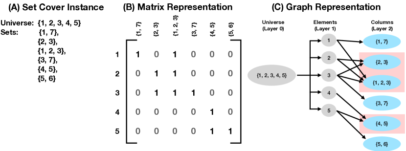
Figure 1. (A) A simple example of a set cover problem. Here, each subset has an equal cost. (B) The set cover instance represented in the covering matrix format. (C) The set cover instance represented in graph format. This graph is passed into a GNN to learn predictions of a subset of nodes/sets important to solving SCP (highlighted in pink). The prediction values for Layer 0 and Layer 1 nodes (grey-colored nodes) are discarded, since only Layer 2 nodes contribute to the solution.

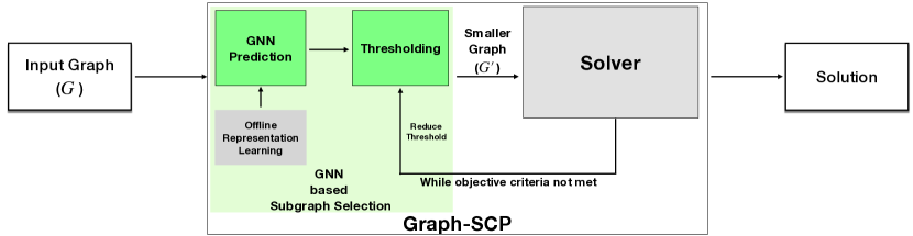
Figure 2. Overall system diagram for Graph-SCP. A GNN is trained offline to predict a subgraph of nodes that contain the solution to the SCP instance. At run time, the GNN is used (only once) to generate predictions. Graph-SCP picks nodes at a set percentile threshold as the subgraph. If the objective criteria is not met, the threshold is decreased, thereby selecting a larger subgraph.

2. Problem Definition and Methods

2.1. Set Cover Problem

Given a binary matrix $A\in\mathbf{R}^{m\times n}$, the set cover problem is defined as covering all $m$ rows by the minimum cost subset of the $n$ columns. Costs of each column are represented in the column vector $c\in\mathbf{R}^{n\times 1}$. An example of such a covering matrix is shown in Figure 1(B). More formally,

(1) $$x_{j}=\begin{cases}1&\text{if column $j$ is in solution}\\ 0&\text{otherwise}\\ \end{cases}\forall j\in n$$

(2) $$\text{minimize}\sum_{{j\in n}}c_{j}x_{j}$$

(3) $$s.t.\ \sum_{j\in n}A_{ij}x_{j}\geq 1,\text{ }\forall i\in m$$

(4) $$x_{j}\in\{0,1\}.$$

Given such a matrix, we can then define its density as

(5) $$d=\frac{q}{m\times n},$$

where $q$ is the number of non-zero entries in the matrix $A$ (Lan et al., 2007).

Given an instance of SCP, we represent the SCP instance as a directed graph by treating the covering matrix as an adjacency matrix with elements in the universe as rows and sets as columns (Figure 1(C)). For the remainder of this section, we adopt a slightly different framing of SCP for pedagogy. Concretely, given a set of elements $\{1,2,\dots m\}$ (called the universe) and a collection of $n$ sets whose union equals the universe, the set cover problem is to identify a sub collection of the $n$ sets whose union equals the universe (Figure 1(A)). A universe node is added to the graph abstraction discussed above, with directed edges from the universe node to each element node that needs to be covered as shown in Figure 1(C). Observe how this creates a directed tripartite graph representation. For each node in this graph, we also consider the following features:

• Cost of each column node, representing the cost of the corresponding subset, with costs of universe and element nodes set to 0.

• Layer (or category) of each node. We use a binary indicator variable, with the value set to 1 for the universe and element nodes and 0 for nodes representing the subsets.

• Cover, i.e., the number of elements of the universe covered by each subset node.

In the next section, we discuss our approach to reducing the SCP problem size by framing it as a subgraph selection learning task,

2.2. Graph-SCP

The field of graph representation learning has demonstrated the important role of learned features in improving many inference tasks on graphs. We explore if learned features can similarly reveal important structure about the SCP solution space. In particular we are interested to understand if nodes that fall in the optimal solution are easy to separate in some learned feature space. Figure 2 shows a high level summary of Graph-SCP, which is discussed in detail below.

2.2.1. Subgraph Selection Task

Given the previously described graph abstraction of the SCP problem, we aim learn offline, a GNN model to predict which subset of nodes are relevant to the solution. More formally, given a graph $G$ with node features $X$, we learn a GNN function $f(G,X)$ to predict a classification vector $y\in\{0,1\}$, where 1 indicates nodes in the subgraph which still contain the SCP solution and 0 otherwise. To generate training data, we solve instances using Gurobi, a state-of-art CO solver and label the subsets ( i.e., nodes in our graph abstraction) that are part of the solution as 1 with all other subsets labelled as 0.

2.2.2. Thresholding

The trained GNN model outputs continuous values between 0 and 1. In order to select a subset of nodes, Graph-SCP selects nodes at a predefined percentile threshold and passes the selected nodes into a CO solver. In our experiments, we demonstrate using Gurobi, however other solvers of choice can be used. Graph-SCP checks if the objective value returned by the solver with the reduced problem size is at least a user-defined optimal objective value opt. If not, the percentile threshold is reduced, thereby selecting a larger set of nodes and passing it into the solver. The selection of the initial threshold has an impact on the run time performance as well as the quality of the solution obtained. For our experiments, we considered to illustrate with opt=95%, however depending on the desired trade-off between solution quality and run-time other threshold choices might be more appropriate. The impact of varying initial thresholds are discussed in the Results section in Figure 8.

2.2.3. Experimental Setup

We experiment with several popular GNN architectures including Graph Attention Networks (GAT) (Veličković et al., 2018), a vanilla Graph Convolutional Network (GCN) (Kipf and Welling, 2016), GraphSAGE (Hamilton et al., 2017) and Chebyshev GCN (Defferrard et al., 2016). Details of a comparative study between architectures are discussed in the Results section (Figure 7).

For the remainder of this work, we use the best performing architecture, the Graph Attention Network (GAT) with two graph attention layers (64 and 128 attention heads respectively) followed by 3 dense fully connected layers with 128 nodes in each layer. We use batch normalization and dropout layers with dropout probability of 60% after each layer.

A binary cross-entropy loss is used to train the model. Interestingly, we notice that the model generalises better if trained for fewer epochs per SCP instance with repeated passes over the instances. Thus, instead of a single pass with a larger number of epochs, we train every instance for 250 epochs with two passes over the dataset.

To generate training data and demonstrate the generalizability of Graph-SCP, we generate instances with various densities and characteristics. We also use the canonical OR Library (Beasley, 1990) at the testing stage. The instances generated for training reflect the OR library in range of densities, number of columns, and number of rows, but incorporate additional variation in the distribution of costs. We categorize the instances into 5 instance types and show results for each:

• Instance Type 1: These instances have costs picked uniformly between {50, 100 200}, with densities around 0.2.

• Instance Type 2: These instances have equal costs for all sets and have densities between 0.1 and 0.2.

• Instance Type 3: These instances are similar to Instance Type 1, but with lower densities around 0.1 and costs picked using a Poisson distribution with $\lambda=20$.

• Instance Type 4: These instances have costs picked using a Poisson distribution with $\lambda=20$ and have a lower density ranging around 0.04.

• Instance Type 5: These instances were picked from the OR Library (Beasley, 1990). We use 10 sets of instances defined in the OR Library (4, 5, 6, A, B, C, D, NRE, NRF and NRG), each with their own characteristics. These instances are not used as training data, but are kept aside for testing only. Details on each set as well as results of Graph-SCP on these sets are shown in Table 2.

Detailed characteristics of each instance type are shown in Table 1. Graph-SCP was trained using 75 instances from each type for a total of 300 instances, excluding Instance Type 5. The test set consists of 30 instances from each type.

Instance Type	$m$	$n$	$z$	$d$	Cost
Instance Type 1	100–400	100–1000	50–250	0.22–0.29	Uniform Random {50, 100, 200}
Instance Type 2	100–300	100–500	20–60	0.16–0.28	Equal
Instance Type 3	200–350	300–350	45–55	0.13–0.18	Poisson ($\lambda=20$)
Instance Type 4	200	1000–3000	4–5	0.04–0.05	Poisson ($\lambda=20$)
Instance Type 5 (OR Library)	100–500	1000–5000	10–140	0.02–0.2	1–100

Table 1. Characteristics of SCP instances used during training and testing of Graph-SCP. Here, $m$ is the number of rows, $n$ the number of columns, $z$ the number of non-zero entries per column and $d$ is the density of the instance. Instance Types 1, 2 and 3 have densities in the range of 10–20% with Instance Type 4 having low densities in the range of 4–5%. Instance Type 5 were picked from the OR Library (Beasley, 1990) and have a wide range of densities from 2–20%. Costs of each column for Instance Type 5 were picked from the OR dataset. Further details of the sets within the OR Library and their results are shown in Table 2

2.2.4. Baseline Methods

We test Graph-SCP in terms of run time speedup and achieved objective value against three baseline approaches. We compare against Gurobi, a state-of-art CO solver. We also compare Graph-SCP to a simple greedy baseline, where the subset with the largest number of uncovered elements is picked at each step. The greedy baseline has faster run times but has an approximation ratio of $ln(n)$ where $n$ is the size of the universe (Chvatal, 1979). As a sanity check for the subgraph selection step and to understand the contribution of learning from solved SCP instances, we also test against a random node selection strategy, where given an initial relative subgraph size parameter $k$, we randomly select $k\%$ nodes to pass to the CO solver. For our experiments, we consider $k=\{20,50,80\}$ of the nodes.

3. Results

Figure 3 shows speed-up performance and solution quality of Graph-SCP, greedy and random subgraph selection baselines relative to Gurobi’s performance (Note, speedups are shown in the log scale). Recall that for these experiments, we chose the minimum objective value for Graph-SCP at 95%, however, as shown in Figure 3, we see that Graph-SCP achieves well over 95% of the optimal objective across all instances, reaching 100% for Instance Type 2 (B) and over 98% for Instance Types 3 and 5 ((C) and (D)). In terms of speedup, we see the largest speedup of about 25x for Instance Type 1 (A) and the smallest speedup of about 1.4x for Instance Type 5 (E).

Instance Type 5 are instances from the OR Library (Beasley, 1990) that are split into different sets based on their characteristics. Shown in (E) are results averaged across all sets. A detailed breakdown of the characteristics of these sets and the performance of Graph-SCP on each set is shown in Table 2. These results highlight the ability of Graph-SCP to generalise to other instances given that Instance Type 5 was not part of the training set.

Note that the greedy algorithm runs significantly faster across all 5 instances, however with poor objective values. In each subplot, the area of the plot above the red line (random subgraph selection baseline) corresponds to the benefits of learning offline strategies for picking a smaller problem size that contains the solution. Observe how the slope of the line causes random selection to perform poorly if a better objective is required. Significant reduction in problem sizes are shown in Figure 4.

Finally, we highlight additional generalizability properties of Graph-SCP by testing against problem instances with increasing size complexity. Similar to (Gasse et al., 2019), we test against instances with number of columns ranging from 1000-5000 with results shown in Figure 5. Note, we use the same model trained on Instance Types 1-4 (with a maximum of 400 rows). Costs were set using a uniform distribution between $[0,100]$. Graph-SCP achieves optimal value for all instances in this experiment while maintaining an average of 1.35x run time improvement.

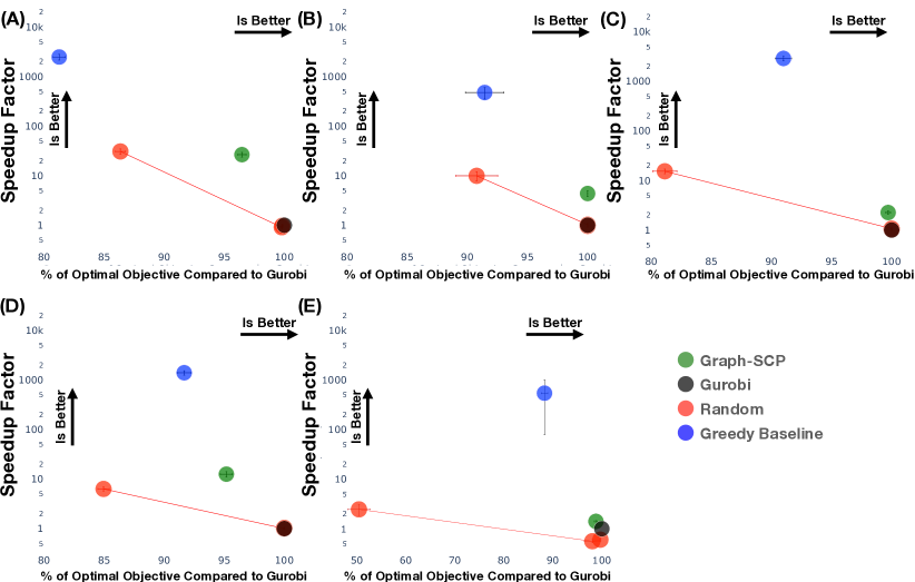
Figure 3. (A) Instance Type 1 (B) Instance Type 2 (C) Instance Type 3 (D) Instance Type 4 (E) Instance Type 5. Across all 5 instances, we see that Graph-SCP achieves over 95% of the optimal objective, reaching 100% for Instance Type 2 (B) and over 98% for Instance Types 3 and 5 ((C) and (D)). In terms of speedup, we see the largest speedup of about 25x for Instance Type 1 (A) and the smallest speedup of about 1.4x for Instance Type 5 (E). Instance Type 5 are instances from the OR Library (Beasley, 1990) that are split into different sets based on their characteristics. Shown in (E) are results averaged across all sets. A detailed breakdown of these sets is shown in Table 2. Note that the greedy algorithm runs significantly faster across all 5 instances, however with poor objective values. In each subplot, the area of the plot above the red line (random sample) correspond to the benefits of learning. Also, observe that Graph-SCP has tight variances compared to the baselines.

Set	# Instances	$m$	$n$	Cost	$d$	% Opt Reached	Speedup	Gurobi Mean	Size
						by Graph-SCP	Factor	Run Time (s)	Reduction
4	10	200	1000	1–100	0.02	96%	0.95	0.067	52%
5	10	200	2000	1–100	0.02	95%	1.34	0.11	55%
6	5	200	1000	1–100	0.05	99%	2.09	0.2	64%
A	5	300	3000	1–100	0.02	100%	1.71	0.37	67%
B	5	300	3000	1–100	0.05	98%	1.42	0.74	67%
C	5	400	4000	1–100	0.02	100%	1.52	0.78	34%
D	5	400	4000	1–100	0.05	100%	1.22	1.63	56%
NRE	5	500	5000	1–100	0.1	100%	1.09	10.1	45%
NRF	5	500	5000	1–100	0.2	100%	1.72	16.04	67%
NRG	5	1000	10000	1–1000	0.02	100%	1.16	515.8	23%

Table 2. Shown above are the sets of instances defined in the OR Library (Beasley, 1990). Each set (4, 5, A, B, NRE etc.) has its own definitive characteristics, as shown in the table. Here, $m$ is the number of rows, $n$ the number of columns and $d$ is the density of the instance. Graph-SCP achieves an average speedup of 1.4x across all sets while achieving over 98% of the optimal objective on average and  50% reduction in problem size

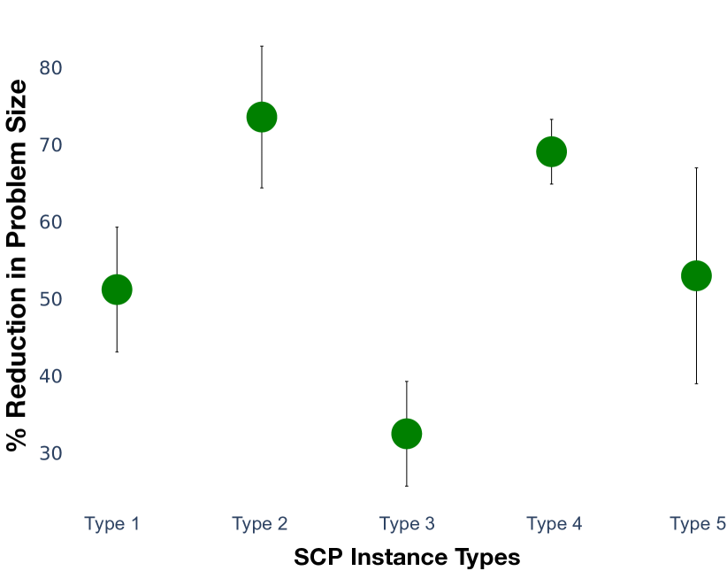
Figure 4. Reduction in problem size achieved by Graph-SCP. We see an average reduction of  50% across all instance types, with the largest reductions seen in Instance Type 2.

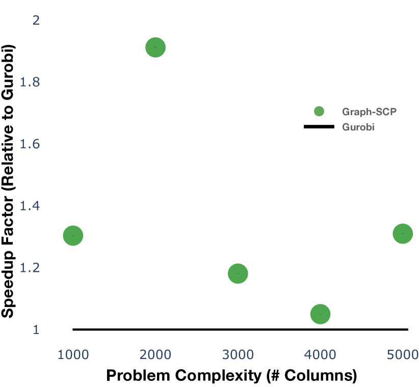
Figure 5. Generalization properties of Graph-SCP against problem instances with increasing complexity (i.e., different instance sizes). Following (Gasse et al., 2019), we test against instances with number of columns ranging from 1000-5000. Note, we use the same model trained on instance of Types 1 through 4, with a much smaller number of rows at a maximum of 400. Costs were set using a uniform distribution between $[0,100]$. Graph-SCP achieves optimal value for all instances in this experiment.

Next, we run several ablation and comparative studies to understand the impact of our modelling choices. We show representative results using Instance Type 1, with results for other Instance Types omitted due to space constraints.

3.1. Node Feature Study

To arrive at the most predictive set, we train and test 4 models with all combinations of the node features (we always include cost as a feature) on Instance Type 1. Results shown here were found to generalize to other instance types. Results are shown in Figure 6, where the $x-$axis shows the speedup in run time compared to Gurobi as a baseline with the $y-$axis showing the quality of the solution in terms of ratio between the objective value obtained by Graph-SCP and Gurobi. Observe that using Costs and Cover leads to the largest speedup, whereas using all 3 node features leads to the best solution quality. In this work, we chose to use Costs and Cover as the two node features in order to achieve the best speedup.

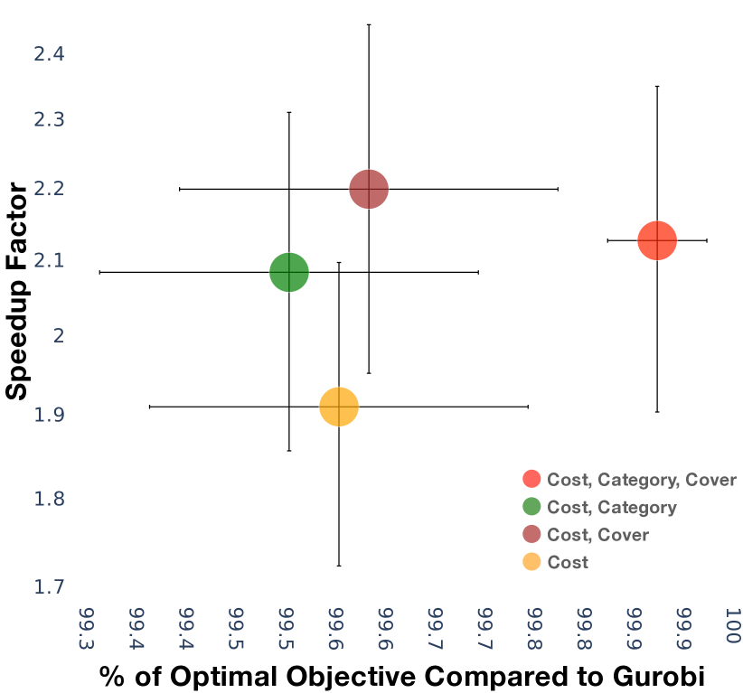
Figure 6. Illustration of Graph-SCP performance using different node features. Costs and Cover (i.e., the number of non-zero entries of each column) features lead to the largest speedup, whereas using all 3 node features leads to the best solution quality. These results belong to Instance Type 1, but were found to generalise to other instance types.

3.2. GNN Architecture Study

We compare 4 commonly used GNN architectures: Graph Attention Networks (GAT) (Veličković et al., 2018), Graph Convolutional Network (GCN) (Kipf and Welling, 2016), GraphSAGE (Hamilton et al., 2017) and Chebyshev GCN (Defferrard et al., 2016). The results of each type of GNN are showed in Figure 7. We observe that every GNN except Chebyshev GCN achieves a faster run time than Gurobi, with GAT achieving the highest speedup at  8x. These architectures were trained on all Instance Types and tested on Instance Type 1 only, with results seen to generalise across test Instance Types (results omitted due to space constraints).

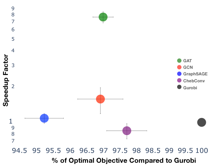
Figure 7. Comparison of different GNN architectures. Observe that every GNN, except Chebyshev GCN, achieves a faster run time than Gurobi, with GAT achieving the highest speedup at  8x. Results were generated from Instance Type 1, but are representative across instances.

3.3. Threshold Sensitivity Analysis

We study the impact of varying the initial threshold on run time and objective performance. Test instances from Instance Type 1 were used with results generalising across Instance Types. Shown in the $y-$axis on the left are the speedups achieved with the $y-$axis on the right showing solution quality. Observe that higher initial thresholds lead to faster run times with lower thresholds leading to better solution quality since a larger portion of the original problem is passed in. Setting the initial threshold too high might lead to multiple calls to the solver after reducing the threshold.

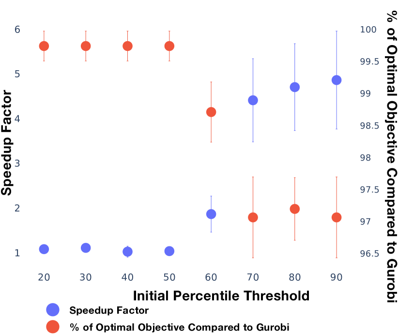
Figure 8. Impact of initial threshold values. Higher thresholds lead to faster run times, while lower thresholds lead to better solution quality since a larger portion of the original problem is passed to the CO solver. Setting the initial threshold too high could lead to multiple calls to the solver after reducing the threshold. We use a reduction rate of 20 throughout the experiments. Results were generated from Instance Type 1 but are representative across instances.

4. Discussions and Limitations

The performance of Graph-SCP depends on the initial threshold as discussed earlier in Figure 8. This threshold needs to be adjusted according to the density and characteristics of the instances.

For instances with small problem sizes, Graph-SCP can be marginally slower than directly solving the problem using a solver, because the overhead of creating and processing the graph is larger than the benefit of reducing the problem size. However, Graph-SCP still achieves a significant reduction in the number of nodes. For larger instances, Graph-SCP is faster than directly solving the problem, because the reduction in the problem size is more substantial. However, when the number of columns is very high, the forward pass through the GNN can be time-consuming and negate the advantage of Graph-SCP.

A possible way to improve Graph-SCP is to use a warm-starting technique, where the solution obtained from the current step is used as an initial guess for the next step, instead of solving each sub-problem from scratch. This could speedup the overall system and reduce the number of iterations. Throughout our experiments, setting the right initial threshold per instance type allowed Graph-SCP to call Gurobi only once. However, implementing the ability to warm start could allow one to set higher thresholds allowing Graph-SCP to make multiple calls to Gurobi with progressively larger problem sizes without loss in run-time performance.

5. Related Work

We have recently seen a growth of literature that explores the use of ML to replace or augment traditional solvers to various CO problems with the objective of accelerating run times, and where appropriate, to improve solution quality. Surveys by Bengio et al. (Bengio et al., 2021) and Cappart et al. (Cappart et al., 2023) provide a detailed summary of this ongoing research Under the approach category that uses ML to replace a CO solver, Numeroso et al. (Numeroso et al., 2023) apply the Neural Algorithmic Reasoning framework proposed by Veličković et al. (Veličković and Blundell, 2021) to jointly optimize for the primal and dual of a given problem. Specifically, they look at training models to find joint solutions for both the min cut and the max flow formulations and show that it leads to better overall performance. For NP-hard problems, Khalil et al. (Khalil et al., 2017) propose a reinforcement learning approach that utilizes graph embeddings to learn a greedy policy that incrementally builds a solution. The aim of our work, was to focus on augmenting and accelerating an existing solver allowing us to carry over any of the performance guarantees that come along with such solvers.

As part of approaches that use ML to aid conventional solvers, Gasse et al. (Gasse et al., 2019) use a GNN to learn expensive to compute branch-and-bound heuristics for Mixed Integer Program (MIP) solvers. The learning is done offline and the learned models are then used at run time in place of the heuristic to achieve faster run times while maintaining the quality of the solution. This work is similar to our approach in that it uses ML to aid a CO solver, however, it does so by speeding up the internal workings (branching heuristic) of the solver. Graph-SCP differs in that it reduces the input problem size complexity, and thereby can be used in conjunction with the method proposed by Gasse et al. to potentially achieve further improvements in run-time. Kruber et al. (Kruber et al., 2017) use supervised learning (e.g., KNN, RBF) to determine when a Dantzig-Wolfe decomposition should be applied to a MIP.

6. Conclusion

We present Graph-SCP, a GNN method that can augment conventional or ML-augmented optimization solvers by learning to identify a much smaller sub-problem containing the solution space. In doing so, Graph-SCP achieves faster run times while still taking advantage of performance guarantees that come along with conventional solutions. Given a desired optimality threshold, Graph-SCP will improve upon it or even achieve 100% optimality with up to  25x faster run times. Unlike most ML solutions for CO, the GNN prediction module within Graph-SCP needs to be run only once. We show that Graph-SCP can generalize across SCP instances with diverse characteristics and complexities and show that it performs well on instances from the canonical OR Library. Through various ablation studies we provide insights on how the different modeling choices affect Graph-SCP performance.

References

- (1)
- Beasley (1990) John E Beasley. 1990. OR-Library: distributing test problems by electronic mail. Journal of the operational research society 41, 11 (1990), 1069–1072.
- Bengio et al. (2021) Yoshua Bengio, Andrea Lodi, and Antoine Prouvost. 2021. Machine learning for combinatorial optimization: A methodological tour d’horizon. European Journal of Operational Research 290, 2 (2021), 405–421.
- Cappart et al. (2023) Quentin Cappart, Didier Chételat, Elias B Khalil, Andrea Lodi, Christopher Morris, and Petar Velickovic. 2023. Combinatorial optimization and reasoning with graph neural networks. J. Mach. Learn. Res. 24 (2023), 130–1.
- Chvatal (1979) Vasek Chvatal. 1979. A greedy heuristic for the set-covering problem. Mathematics of operations research 4, 3 (1979), 233–235.
- Defferrard et al. (2016) Michaël Defferrard, Xavier Bresson, and Pierre Vandergheynst. 2016. Convolutional neural networks on graphs with fast localized spectral filtering. Advances in neural information processing systems 29 (2016).
- Gasse et al. (2019) Maxime Gasse, Didier Chételat, Nicola Ferroni, Laurent Charlin, and Andrea Lodi. 2019. Exact combinatorial optimization with graph convolutional neural networks. In NeurIPS.
- Gurobi Optimization, LLC (2023) Gurobi Optimization, LLC. 2023. Gurobi Optimizer Reference Manual. https://www.gurobi.com
- Hamilton et al. (2017) Will Hamilton, Zhitao Ying, and Jure Leskovec. 2017. Inductive representation learning on large graphs. Advances in neural information processing systems 30 (2017).
- Khalil et al. (2017) Elias Khalil, Hanjun Dai, Yuyu Zhang, Bistra Dilkina, and Le Song. 2017. Learning combinatorial optimization algorithms over graphs. In NeurIPS.
- Kipf and Welling (2016) Thomas N Kipf and Max Welling. 2016. Semi-supervised classification with graph convolutional networks. arXiv preprint arXiv:1609.02907 (2016).
- Kruber et al. (2017) Markus Kruber, Marco E Lübbecke, and Axel Parmentier. 2017. Learning when to use a decomposition. In International conference on AI and OR techniques in constraint programming for combinatorial optimization problems. Springer, 202–210.
- Lan et al. (2007) Guanghui Lan, Gail W DePuy, and Gary E Whitehouse. 2007. An effective and simple heuristic for the set covering problem. European journal of operational research 176, 3 (2007), 1387–1403.
- Numeroso et al. (2023) Danilo Numeroso, Davide Bacciu, and Petar Veličković. 2023. Dual algorithmic reasoning. In ICLR.
- Veličković and Blundell (2021) Petar Veličković and Charles Blundell. 2021. Neural algorithmic reasoning. Patterns 2, 7 (2021), 100273.
- Veličković et al. (2018) Petar Veličković, Guillem Cucurull, Arantxa Casanova, Adriana Romero, Pietro Liò, and Yoshua Bengio. 2018. Graph attention networks. In ICLR.