The APOGEE Value Added Catalogue of Galactic globular cluster stars

Abstract

We introduce the SDSS/APOGEE Value Added Catalogue of Galactic Globular Cluster (GC) Stars. The catalogue is the result of a critical search of the APOGEE data release 17 (DR17) catalogue for candidate members of all known Galactic GCs. Candidate members are assigned to various GCs on the basis of position on the sky, proper motion, and radial velocity. The catalogue contains a total of 7,737 entries for 6,422 unique stars associated with 72 Galactic GCs. Full APOGEE DR17 information is provided, including radial velocities and abundances for up to 20 elements. Membership probabilities estimated on the basis of precision radial velocities are made available. Comparisons with chemical compositions derived by the GALAH survey, as well as optical values from the literature, show good agreement. This catalogue represents a significant increase in the public database of GC star chemical compositions and kinematics, providing a massive homogeneous data set that will enable a variety of studies. The catalogue in fits format is available for public download from the SDSS-IV DR17 value added catalogue website.

1 Introduction

Globular clusters are intriguing objects. The physics of their genesis is not entirely understood, yet their study has advanced knowledge in several fields of astrophysics. The mapping of the spatial distribution of Galactic globular clusters (GCs) promoted a radical revision of the position of the solar system in the universe (Shapley, 1918); application of the physics of stellar structure and evolution to GC observations constrained the age of the universe in the early days of Big Bang cosmology (e.g., Sandage, 1970; Bolte & Hogan, 1995, and references therein); GC ages, chemical compositions, and orbital properties provide important clues to the star formation and accretion history of the early Milky Way (e.g., Searle & Zinn, 1978; Salaris & Weiss, 2002; Massari et al., 2019; Kruijssen et al., 2019; Horta et al., 2020; Forbes, 2020; Callingham et al., 2022) as well as other galaxies (Brodie & Strader, 2006, and references therein); finally and no less crucially, to this day GCs are fundamental test beds of stellar evolution theory in the low mass regime (e.g., Schwarzschild, 1970; Renzini & Fusi Pecci, 1988; Chiosi et al., 1992; Salaris et al., 2002). Yet after over a century of study, their origin is still subject to debate, with no shortage of formation scenarios (e.g., Fall & Rees, 1985; Schweizer, 1987; Ashman & Zepf, 1992) despite recent encouraging progress (e.g., Kruijssen, 2015; Choksi et al., 2018; Pfeffer et al., 2018).

Since GCs stand at the crossroads of many areas of astrophysics, it is small wonder that they have been subject to various herculean observational efforts over the past several decades—in fact so many that an exhaustive account is rendered impossible in this brief introduction. We thus limit ourselves to mention a few highlights and some of the most recent work, in a manner dictated by the authors’ own personal biases and an unavoidably limited grasp of an overwhelming—and ever growing—literature.

Systematic photometric observations built ground and space based colour-magnitude diagrams of large GC samples in the optical (e.g., Barbuy et al., 1998; Rosenberg et al., 2000; Piotto et al., 2002; Sarajedini et al., 2007; Stetson et al., 2019), near infrared (e.g., Cohen et al., 2017; Minniti et al., 2017), and ultraviolet (e.g., Schiavon et al., 2012; Sahu et al., 2022). Libraries of integrated spectra were created for comparison against observations of extragalactic GCs and reality checking of stellar population synthesis models (e.g., Zinn & West, 1984; Bica & Alloin, 1986; Armandroff & Zinn, 1988; Puzia et al., 2002; Schiavon et al., 2005), and more recently integral field spectroscopy of large GC samples have also become available (e.g., Usher et al., 2017; Kamann et al., 2018). In this context, the GC system of the Andromeda galaxy has also become subject to extensive integrated light surveys both in optical and NIR (e.g., Galleti et al., 2007; Caldwell et al., 2009; Schiavon et al., 2013; Sakari et al., 2016). Finally, with the advent of the Gaia satellite, a massive undertaking by E. Vasiliev and H. Baumgardt has produced precision kinematics and structural parameters for the vast majority of known Galactic GCs (Baumgardt & Vasiliev, 2021; Vasiliev & Baumgardt, 2021).

Chemical compositions of individual GC stars constitute precious, and quite expensive, information for a variety of scientific pursuits. Within the confines of stellar evolution theory, such pursuits include the calibration of evolutionary tracks, the study of stellar evolution processes such as dredge up and deep mixing along the giant branch (e.g., Kraft, 1979; Shetrone, 1996), and diffusion of heavy elements in main sequence stars (e.g., Denissenkov & Weiss, 1996; Castellani & degl’Innocenti, 1999; Lind et al., 2008). The first systematic collection of chemical compositions of individual stars in Galactic GCs was conducted by the Lick/Texas group (e.g., Kraft, 1994; Shetrone, 1996; Sneden et al., 1997). Contrary to the generally agreed notion of GCs as coeval stellar systems with homogeneous chemical compositions, these early efforts revealed that star-to-star abundance variations are ubiquitous. These were difficult to understand, but since the data were restricted to bright giant stars, the broad consensus was that such variations should be ascribed to stellar evolution effects.

The next generation of systematic measurements brought about a considerable amplification of the existing database of homogeneously derived chemical compositions (e.g., Carretta & Gratton, 1997; Carretta et al., 2010, and references therein). These efforts consolidated the knowledge that star-to-star chemical composition variations are the norm in GCs. They typically manifest themselves in the form of anti-correlations between the abundances of light elements such as C-N, Na-O, and Mg-Al (e.g., Gratton et al., 2012). Such abundance variations are present in main sequence stars (e.g., Cannon et al., 1998), ruling out evolutionary effects as their physical origin. In addition to these features, massive systems such as $\omega$ Cen, among others, display variations in the abundances of the heavy elements that are by-products of SN Ia enrichment (e.g., Pancino et al., 2002; Johnson & Pilachowski, 2010).

The discovery of multiple sequences in colour-magnitude diagrams, made possible by the significant increase in photometric precision afforded by the HST/ACS, prompted the conclusion that GCs host a complex mix of stellar populations. In view of this overwhelming evidence, the historical assumption that GCs are single stellar populations had to be dropped. This so called multiple populations phenomenon, is without a doubt inextricably linked to the physics of GC formation. Yet no formation scenarios are capable of accounting for this phenomemon in a quantitative fashion (see reviews by Renzini et al., 2015; Bastian & Lardo, 2018; Milone & Marino, 2022).

A solution to the problem of multiple populations in GCs, and in a broader perspective our understanding of the nature of these beautiful and fascinating systems, can be advanced by the production of a massive, homogeneous, and publicly available database of chemical compositions and kinematics for a large sample of Galactic GCs. This paper summarises the effort by the APOGEE team to make one such database available to public access. We present the APOGEE value added catalogue (VAC) of Galactic globular cluster members. The paper is organised as follows. In Section 2 we briefly describe the APOGEE data. In Section 3 the criteria adopted for selecting candidate GC members are described, while membership probabilities are discussed in Section 4. Broad features of the data are presented in Section 5, and Section 6 describes the catalogue and provides access information.

2 The data

This paper presents a catalogue of chemical compositions and radial velocities from the latest data release of the SDSS-IV/APOGEE 2 survey (DR17, Majewski et al., 2017; Abdurro’uf et al., 2022). Proper motions from the early third data release (eDR3) from the Gaia satellite (Gaia Collaboration et al., 2021) and various additional metadata imported directly from the DR17 catalogue are also included for convenience sake. Data from APOGEE have been described in detail in various technical publications, so we provide a brief account of their main properties in this Section, referring the reader to the relevant papers for further details. Chemical-composition data based on earlier APOGEE data releases were presented for various collections of Galactic GCs in a number of publications (e.g., Mészáros et al., 2015; Schiavon et al., 2017b; Nataf et al., 2019; Masseron et al., 2019; Mészáros et al., 2020, 2021; Geisler et al., 2021).

Elemental abundances and radial velocities are obtained from the automatic analysis of moderately high-resolution near-infrared spectra of hundreds of thousands of stars observed with the Apache Point Observatory 2.5 m Sloan telescope (Gunn et al., 2006) and the Las Campanas Observatory 2.5 m Du Pont telescope Bowen & Vaughan (1973). The telescopes are equipped with twin high efficiency multi-fiber NIR spectrographs designed and assembled at the University of Virginia, USA (Wilson et al., 2019). A technical summary of the overall SDSS-IV experiment can be found in Blanton et al. (2017).

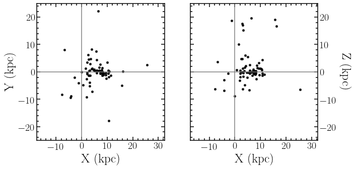
Figure 1: Spatial distribution of the GCs included in this VAC, in Cartesian coordinates with the Sun at the origin (cross hairs). The sample is preferentially concentrated towards the inner Galaxy.

APOGEE spectra for any given star (save for a relatively small number of exceptions) were obtained in a number of visits separated in time to enable the detection of radial velocity variations caused by binarity. Observations spanned a period of typically 3 months, never exceeding 6 months between first and last visit. Every visit spectrum was integrated typically for $\sim$1 hour in sets of four (ABBA) exposures taken with the detector dithered along the spectral direction. Spectral dithers were aimed at bringing the sampling of the line spread function to slightly better than critical in the blue end of the spectrum where the sampling by the detector’s original pixel size is sub-critical.

A pipeline built specifically for the reduction of APOGEE data (Nidever et al., 2015) was employed to apply standard operations such as reference pixel voltage correction, linearisation, cosmic-ray and saturation corrections, dark current subtraction, persistence correction, and extraction of the 2D data array from the 3D data cubes. The 2D images were then flat-field corrected and a bad-pixel mask was generated before 1D spectra were extracted, and subsequently wavelength and flux calibrated. The next step was to subtract the sky background, which is dominated by emission lines, and perform telluric correction before combining the dithered sequences into a single well sampled resulting visit spectrum.

For each star, relative radial velocities of visit spectra were measured through iterative cross correlation with the combined spectrum, and final absolute RVs are then obtained by cross-correlation of the combined spectrum with a grid of synthetic spectra covering a wide range of stellar parameters. The resulting combined restframe spectrum is that which is finally fed into the stellar abundances pipeline.

The APOGEE Stellar Parameters and Chemical Abundances Pipeline (ASPCAP) is described in detail by García Pérez et al. (2016) and later updates (Holtzman et al., 2018; Jönsson et al., 2020). In short, it determines stellar parameters and detailed elemental abundances through interpolation, using the FERRE software (Allende Prieto et al., 2006), into a huge grid of synthetic spectra covering the entire range of stellar parameters and chemical compositions of interest. The spectral library is calculated adopting MARCS model atmospheres (Gustafsson et al., 2008) generated specifically for the purposes of the APOGEE survey (see Mészáros et al., 2012; Zamora et al., 2015; Holtzman et al., 2018; Jönsson et al., 2018). ASPCAP abundance analysis is based on various flavours of line lists, depending on the spectrum synthesis codes, LTE/non-LTE assumption, and model atmospheres adopted in the construction of the spectral library. Those line lists are empirically tuned to match the observed high-resolution spectra of the Sun and Arcturus. For details, see Smith et al. (2021) (but see also Cunha et al., 2017; Hasselquist et al., 2016; Shetrone et al., 2015).

The data described above were made publicly available in data release 17 in the form of various catalogues for different flavours of spectral analysis, according to the spectrum synthesis code adopted in the construction of the spectral library, adoption or not of an NLTE approach for some elements, and the assumption of plane-parallel or spherical geometry in the radiative transfer calculation. Each catalogue contains 733,901 entries. The data contained in this VAC are extracted from the default DR17 data analysis, which is based on the Synspec-based (Hubeny & Lanz, 2017) spectral library, with incorporation of an NLTE abundance analysis for elements Na, Mg, K, and Ca (prefix synspec_rev1, see Osorio et al., 2020, and references therein).

2.1 Globular Cluster Sample

Globular clusters were targeted by APOGEE so as to satisfy at the same time scientific interests and calibration needs. As the first attempt at automatic detailed chemical composition analysis of a massive near infrared spectroscopic database, optical calibrators are a crucial requirement for APOGEE. As targets of interest for various scientific pursuits, GC stars have for decades been the focus of chemical composition studies. Thus the availability of multiple elemental abundance determinations in the literature, overwhelmingly based on optical spectroscopy, placed GC stars at the centre of the APOGEE calibration procedure (e.g., Holtzman et al., 2015, 2018; Jönsson et al., 2020). With those goals in mind, a large number of GCs were targeted during the execution of both APOGEE 1 and 2. Targets within each GC were selected to meet a set of criteria whereby stars that were subject to previous abundance analysis and/or atmospheric parameter determinations were given top priority, followed by stars with membership confirmed on the basis of radial velocity, proper motion, and position on the colour-magnitude diagram, in decreasing order of priority (for details, see Zasowski et al., 2013, 2017; Santana et al., 2021; Beaton et al., 2021). In addition to the GCs targeted as part of the main APOGEE survey, a number of additional systems were observed as part of the bulge Cluster APOgee Survey (CAPOS, Geisler et al., 2021). The CAPOS team took advantage of Chilean access to the APOGEE South spectrograph (Wilson et al., 2019) to collect data for a number of GCs located towards the inner Galaxy. CAPOS spectra were collected, reduced and analysed following the same procedures and pipelines as the main survey targets, with results being ingested into the SDSS/APOGEE database. Data obtained by CAPOS are thus treated in this paper in the same way as the targets from the main APOGEE survey. Table 2 lists the GCs included in this value added catalogue, along with basic parameters, extracted from Baumgardt & Vasiliev (2021); Vasiliev & Baumgardt (2021), which we hereafter refer simply as the VB catalogue. The number of candidate members of each GC is also listed. The distribution of our GC sample in Cartesian coordinates is shown in Figure 1. Unfortunately, GCs whose discovery was reported after the latest update of the VB catalogue, such as VVV CL001 (Fernández-Trincado et al., 2021b) and Patchick 125 (Fernández-Trincado et al., 2022) are not included in this catalogue, but will be incorporated in future versions.

Table 1: Globular clusters included in the sample. Column information: (1) GC ID; (2,3) coordinates of GC centre; (4) mean iron abundance; (5) mean radial velocity; (6) heliocentric distance; (7) Galactocentric distance; (8) mass; (9) Jacobi radius; (10) number of entries. Numbers for columns 2, 3, 5, 6, 7, 8, and 9 are from the VB catalogue, whereas those for columns 4 and 10 are from this work.

GC	$\alpha_{\rm cen}$	$\delta_{\rm cen}$	$\langle{\rm\lceil Fe/H\rceil}\rangle$	$\langle{\rm R.V.}\rangle$	$d_{\odot}$	$R_{\rm GC}$	Mass	$r_{\rm J}$	N
	deg	deg		km s-1	kpc	kpc	104 M⊙	deg
NGC 104	6.02379	-72.08131	-0.74	-17.45 $\pm$ 0.16	4.52 $\pm$ 0.03	7.52 $\pm$ 0.01	89.5 $\pm$ 0.6	1.557	297
NGC 288	13.18850	-26.58261	-1.27	-44.45 $\pm$ 0.13	8.99 $\pm$ 0.09	12.21 $\pm$ 0.06	9.3 $\pm$ 0.3	0.605	43
NGC 362	15.80942	-70.84878	-1.11	223.12 $\pm$ 0.28	8.83 $\pm$ 0.10	9.62 $\pm$ 0.06	28.4 $\pm$ 0.4	0.598	70
Palomar 1	53.33350	79.58105	-0.45	-75.72 $\pm$ 0.29	11.28 $\pm$ 0.32	17.41 $\pm$ 0.29	0.10 $\pm$ 0.02	0.122	3
NGC 1851	78.52816	-40.04655	-1.13	321.4 $\pm$ 1.55	11.95 $\pm$ 0.13	16.69 $\pm$ 0.11	31.8 $\pm$ 0.4	0.611	71
NGC 1904	81.04584	-24.52442	-1.52	205.76 $\pm$ 0.2	13.08 $\pm$ 0.18	19.09 $\pm$ 0.16	13.9 $\pm$ 1.0	0.259	40
NGC 2298	102.24754	-36.00531	-1.84	147.15 $\pm$ 0.57	9.83 $\pm$ 0.17	15.07 $\pm$ 0.14	5.6 $\pm$ 0.8	0.435	12
NGC 2808	138.01291	-64.86349	-1.07	103.57 $\pm$ 0.27	10.06 $\pm$ 0.11	11.58 $\pm$ 0.07	86.4 $\pm$ 0.6	0.944	132
NGC 3201	154.40343	-46.41248	-1.39	493.65 $\pm$ 0.21	4.74 $\pm$ 0.04	8.93 $\pm$ 0.02	16.0 $\pm$ 0.3	0.925	217
NGC 4147	182.52626	18.54264	-1.63	179.35 $\pm$ 0.31	18.53 $\pm$ 0.21	20.2 $\pm$ 0.2	3.9 $\pm$ 0.9	0.274	3
Rup 106	189.66750	-51.15028	-1.30	-38.36 $\pm$ 0.26	20.71 $\pm$ 0.36	18.0 $\pm$ 0.3	3.4 $\pm$ 0.6	0.213	2
NGC 4590	189.86658	-26.74406	-2.22	-93.11 $\pm$ 0.18	10.40 $\pm$ 0.10	10.35 $\pm$ 0.07	12.2 $\pm$ 0.9	0.426	41
NGC 5024	198.23021	18.16817	-1.90	-63.37 $\pm$ 0.25	18.50 $\pm$ 0.18	19.0 $\pm$ 0.16	45.5 $\pm$ 3.0	0.549	41
NGC 5053	199.11288	17.70025	-2.21	42.82 $\pm$ 0.25	17.54 $\pm$ 0.23	18.01 $\pm$ 0.2	7.4 $\pm$ 2.0	0.317	17
NGC 5139	201.69699	-47.47947	-1.60	232.78 $\pm$ 0.21	5.43 $\pm$ 0.05	6.5 $\pm$ 0.01	364 $\pm$ 4	2.142	1864
NGC 5272	205.54842	28.37728	-1.43	-147.2 $\pm$ 0.27	10.17 $\pm$ 0.08	12.09 $\pm$ 0.06	41.0 $\pm$ 1.7	0.714	299
NGC 5466	211.36371	28.53444	-1.81	106.82 $\pm$ 0.2	16.12 $\pm$ 0.16	16.47 $\pm$ 0.13	6.0 $\pm$ 1.0	0.284	17
NGC 5634	217.40533	-5.97643	-1.72	-16.07 $\pm$ 0.6	25.96 $\pm$ 0.62	21.84 $\pm$ 0.57	22.8 $\pm$ 4.0	0.42	2
Palomar 5	229.01917	-0.121	-1.24	-58.61 $\pm$ 0.15	21.94 $\pm$ 0.51	17.27 $\pm$ 0.47	1.0 $\pm$ 0.2	0.12	12
NGC 5904	229.63841	2.08103	-1.21	53.5 $\pm$ 0.25	7.48 $\pm$ 0.06	6.27 $\pm$ 0.02	39.4 $\pm$ 0.6	0.607	259
NGC 6093	244.26004	-22.97608	-1.61	10.93 $\pm$ 0.39	10.34 $\pm$ 0.12	3.95 $\pm$ 0.08	33.8 $\pm$ 0.9	0.344	3
NGC 6121	245.86974	-26.52575	-1.07	71.21 $\pm$ 0.15	1.85 $\pm$ 0.02	6.45 $\pm$ 0.01	8.7 $\pm$ 0.1	1.658	224
NGC 6144	246.80777	-26.0235	-1.80	194.79 $\pm$ 0.58	8.15 $\pm$ 0.13	2.5 $\pm$ 0.02	7.9 $\pm$ 1.4	0.198	1
NGC 6171	248.13275	-13.05378	-1.02	-34.71 $\pm$ 0.18	5.63 $\pm$ 0.08	3.74 $\pm$ 0.04	7.5 $\pm$ 0.4	0.368	65
NGC 6205	250.42181	36.45986	-1.48	-244.9 $\pm$ 0.3	7.42 $\pm$ 0.08	8.64 $\pm$ 0.04	54.5 $\pm$ 2.0	1.036	152
NGC 6229	251.74525	47.5278	-1.24	-137.89$\pm$ 0.71	30.11 $\pm$ 0.47	29.45 $\pm$ 0.44	28.6 $\pm$ 9.0	0.395	11
NGC 6218	251.80907	-1.94853	-1.27	-41.67 $\pm$ 0.14	5.11 $\pm$ 0.05	4.57 $\pm$ 0.02	10.7 $\pm$ 0.3	0.508	107
NGC 6254	254.28772	-4.10031	-1.51	74.21 $\pm$ 0.23	5.07 $\pm$ 0.06	4.35 $\pm$ 0.03	20.5 $\pm$ 0.4	0.611	87
NGC 6273	255.65749	-26.26797	-1.71	145.54 $\pm$ 0.59	8.34 $\pm$ 0.16	1.43 $\pm$ 0.03	69.7 $\pm$ 3.6	0.266	81
NGC 6293	257.54250	-26.58208	-2.09	-143.66$\pm$ 0.39	9.19 $\pm$ 0.28	1.6 $\pm$ 0.18	20.5 $\pm$ 1.6	0.153	20
NGC 6304	258.63440	-29.46203	-0.48	-108.62$\pm$ 0.39	6.15 $\pm$ 0.15	2.19 $\pm$ 0.13	12.6 $\pm$ 1.1	0.276	34
NGC 6316	259.15542	-28.14011	-0.77	99.65 $\pm$ 0.84	11.15 $\pm$ 0.39	3.16 $\pm$ 0.36	32.8 $\pm$ 4.0	0.271	24
NGC 6341	259.28076	43.13594	-2.25	-120.55$\pm$ 0.27	8.50 $\pm$ 0.07	9.84 $\pm$ 0.04	35.2 $\pm$ 0.4	0.808	80
Terzan 2	261.88792	-30.80233	-0.86	134.56 $\pm$ 0.96	7.75 $\pm$ 0.33	0.74 $\pm$ 0.16	13.6 $\pm$ 2.5	0.084	5
Terzan 4	262.66251	-31.59553	-1.38	-48.96 $\pm$ 1.57	7.59 $\pm$ 0.31	0.82 $\pm$ 0.2	20.0 $\pm$ 5.0	0.125	3
HP 1	262.77167	-29.98167	-1.21	39.76 $\pm$ 1.22	6.99 $\pm$ 0.14	1.26 $\pm$ 0.13	12.4 $\pm$ 1.7	0.156	17
FSR 1758	262.8	-39.808	-1.42	227.31 $\pm$ 0.59	11.08 $\pm$ 0.74	3.46 $\pm$ 0.63	62.8 $\pm$ 5.6	0.618	15
Liller 1	263.35233	-33.38956	-0.14	60.36 $\pm$ 2.44	8.06 $\pm$ 0.35	0.74 $\pm$ 0.07	91.5 $\pm$ 14.7	0.261	30
NGC 6380	263.61861	-39.06953	-0.78	-1.48 $\pm$ 0.73	9.61 $\pm$ 0.30	2.15 $\pm$ 0.21	33.4 $\pm$ 0.5	0.233	28
Ton 2	264.03929	-38.54092	-0.74	-184.72$\pm$ 1.12	6.99 $\pm$ 0.33	1.76 $\pm$ 0.19	6.9 $\pm$ 1.6	0.166	11
NGC 6388	264.07178	-44.7355	-0.49	83.11 $\pm$ 0.45	11.17 $\pm$ 0.16	3.99 $\pm$ 0.13	125.0 $\pm$ 1.0	0.516	75
NGC 6401	264.65219	-23.9096	-1.09	-105.44$\pm$ 2.5	8.06 $\pm$ 0.24	0.75 $\pm$ 0.04	14.5 $\pm$ 0.2	0.094	7
NGC 6397	265.17538	-53.67434	-2.02	18.51 $\pm$ 0.08	2.48 $\pm$ 0.02	6.01 $\pm$ 0.02	9.7 $\pm$ 0.1	1.174	187
Palomar 6	265.92581	-26.22499	-0.92	177.0 $\pm$ 1.35	7.05 $\pm$ 0.45	1.33 $\pm$ 0.45	9.5 $\pm$ 1.7	0.124	6
Terzan 5	267.02020	-24.77906	-0.78	-82.57 $\pm$ 0.73	6.62 $\pm$ 0.15	1.65 $\pm$ 0.13	93.5 $\pm$ 6.9	0.422	24
NGC 6441	267.55441	-37.05145	-0.49	18.47 $\pm$ 0.56	12.73 $\pm$ 0.16	4.78 $\pm$ 0.15	132.0 $\pm$ 1.0	0.502	25
UKS1	268.61331	-24.14528	-1.00	59.38 $\pm$ 2.63	15.58 $\pm$ 0.56	7.7 $\pm$ 0.5	7.7 $\pm$ 0.	0.17	5
Terzan 9	270.41167	-26.83972	-1.36	68.49 $\pm$ 0.56	5.77 $\pm$ 0.34	2.46 $\pm$ 0.32	12.0 $\pm$ 1.4	0.295	23
Djorg 2	270.45438	-27.82582	-1.07	-149.75$\pm$ 1.1	8.76 $\pm$ 0.18	0.8 $\pm$ 0.13	12.5 $\pm$ 0.3	0.079	10
NGC 6517	270.46075	-8.95878	-1.58	-35.06 $\pm$ 1.65	9.23 $\pm$ 0.56	3.24 $\pm$ 0.26	19.5 $\pm$ 2.8	0.27	1
Terzan 10	270.74083	-26.06694	-1.62	211.37 $\pm$ 2.27	10.21 $\pm$ 0.40	2.17 $\pm$ 0.37	30.2 $\pm$ 5.6	0.191	2
NGC 6522	270.89198	-30.03397	-1.22	-15.23 $\pm$ 0.49	7.30 $\pm$ 0.21	1.04 $\pm$ 0.17	21.1 $\pm$ 1.3	0.181	15
NGC 6528	271.2067	-30.05578	-0.16	211.86 $\pm$ 0.43	7.83 $\pm$ 0.24	0.7 $\pm$ 0.1	5.7 $\pm$ 0.7	0.067	4
NGC 6539	271.20728	-7.58586	-0.74	35.19 $\pm$ 0.5	8.17 $\pm$ 0.39	3.09 $\pm$ 0.07	20.9 $\pm$ 1.7	0.317	1
NGC 6540	271.53566	-27.76529	-1.02	-16.5 $\pm$ 0.78	5.91 $\pm$ 0.27	2.34 $\pm$ 0.25	3.5 $\pm$ 1.2	0.165	6
NGC 6544	271.83383	-24.99822	-1.52	-38.46 $\pm$ 0.67	2.58 $\pm$ 0.06	5.62 $\pm$ 0.06	9.1 $\pm$ 0.6	1.078	27
NGC 6553	272.31532	-25.90775	-0.19	-0.27 $\pm$ 0.34	5.33 $\pm$ 0.13	2.83 $\pm$ 0.13	28.5 $\pm$ 1.6	0.494	17
NGC 6558	272.57397	-31.76451	-0.99	-195.12$\pm$ 0.73	7.47 $\pm$ 0.29	1.08 $\pm$ 0.17	2.65 $\pm$ 0.08	0.073	6
Terzan 12	273.06583	-22.74194	-0.56	95.61 $\pm$ 1.21	5.17 $\pm$ 0.38	3.17 $\pm$ 0.34	8.7 $\pm$ 2.0	0.312	6

Table 1: Continued

GC	$\alpha_{\rm cen}$	$\delta_{\rm cen}$	$\langle{\rm\lceil Fe/H\rceil}\rangle$	$\langle{\rm R.V.}\rangle$	$d_{\odot}$	$R_{\rm GC}$	Mass	$r_{\rm J}$	N
	deg	deg		km s-1	kpc	kpc	104 M⊙	deg
NGC 6569	273.41167	-31.82689	-0.92	-49.83 $\pm$ 0.5	10.53 $\pm$ 0.26	2.59 $\pm$ 0.23	23.6 $\pm$ 2.0	0.226	14
NGC 6642	277.97596	-23.4756	-1.09	-60.61 $\pm$ 1.35	8.05 $\pm$ 0.20	1.66 $\pm$ 0.01	3.4 $\pm$ 0.1	0.11	12
NGC 6656	279.09976	-23.90475	-1.70	-148.72$\pm$ 0.78	3.30 $\pm$ 0.04	5.0 $\pm$ 0.03	47.6 $\pm$ 0.5	1.308	412
NGC 6715	283.76385	-30.47986	-0.62	143.13 $\pm$ 0.43	26.28 $\pm$ 0.33	18.51 $\pm$ 0.32	178.0 $\pm$ 3.0	0.618	1809
NGC 6717	283.77518	-22.70147	-1.12	30.25 $\pm$ 0.9	7.52 $\pm$ 0.13	2.38 $\pm$ 0.02	3.6 $\pm$ 0.8	0.151	5
NGC 6723	284.88812	-36.63225	-1.02	-94.39 $\pm$ 0.26	8.27 $\pm$ 0.10	2.47 $\pm$ 0.02	17.7 $\pm$ 1.1	0.258	9
NGC 6752	287.7171	-59.98455	-1.47	-26.01 $\pm$ 0.12	4.12 $\pm$ 0.04	5.3 $\pm$ 0.02	27.6 $\pm$ 0.4	0.913	152
NGC 6760	287.80027	1.03047	-0.75	-2.37 $\pm$ 1.27	8.41 $\pm$ 0.43	5.17 $\pm$ 0.14	26.9 $\pm$ 2.5	0.488	11
Palomar 10	289.50693	18.57899	0.02	-31.7 $\pm$ 0.23	8.94 $\pm$ 1.18	7.6 $\pm$ 0.59	16.2 $\pm$ 2.7	0.431	3
NGC 6809	294.99878	-30.96475	-1.76	174.7 $\pm$ 0.17	5.35 $\pm$ 0.05	4.01 $\pm$ 0.03	19.3 $\pm$ 0.8	0.549	98
NGC 6838	298.44373	18.77919	-0.75	-22.72 $\pm$ 0.2	4.00 $\pm$ 0.05	6.86 $\pm$ 0.01	4.6 $\pm$ 0.2	0.619	129
NGC 7078	322.49304	12.167	-2.29	-106.84$\pm$ 0.3	10.71 $\pm$ 0.10	10.76 $\pm$ 0.07	63.3 $\pm$ 0.7	0.757	155
NGC 7089	323.36258	-0.82325	-1.47	-3.78 $\pm$ 0.3	11.69 $\pm$ 0.11	10.54 $\pm$ 0.08	62.7 $\pm$ 1.1	0.548	36

3 Selecting Cluster Member Candidates

The number of stars targeted per GC varied widely as a function of the number of visits, apparent magnitude, and apparent GC size, which constrains the number of possible targets in any given visit by virtue of the fiber collision radius of $\sim$ 1’. Moreover, the fraction of bona fide GC members from previous studies also varies widely across the GC sample, as does the number of targets lacking a previous membership assignment based on radial velocity or proper motion measurement.

Table 2: Definition of two subgroups of candidate members. Column information: (1) Subgroup type; (2) angular distance limits in units of the Jacobi radius, given in Table 1; (3) PM limits; (4) RV limits, (5) $\lceil{\rm Fe/H}\rceil$ limits. Limits in columns (3) to (5) in units of residuals defined as $\delta~{}X=\frac{{\rm res}(X)}{\sigma_{X}}$, where ${\rm res}(X)=|X-\mu_{X}|$, and $\mu_{X}$ and $\sigma_{X}$ stand for the mean and r.m.s. scatter of each observable, respectively.

Subgroup	Distance	PM	RV	$\lceil{\rm Fe/H}\rceil$
(1)	(2)	(3)	(4)	(5)
Likely	$r<r_{\rm J}$	$\delta~{}{\rm PM}<2$	$\delta~{}{\rm RV}<2$	any
Outlier	$r_{\rm J}<r<4~{}r_{\rm J}^{\star}$	$2<\delta~{}{\rm PM}<10$	$2<\delta~{}{\rm RV}<3$	$\delta~{}\lceil{\rm Fe/H}\rceil<2$

• ^⋆ For GCs located in crowded fields towards the inner Galaxy, the initial search radius was reduced from 4 $r_{\rm J}$ to 2 $r_{\rm J}$, in order to minimise contamination by field stars.

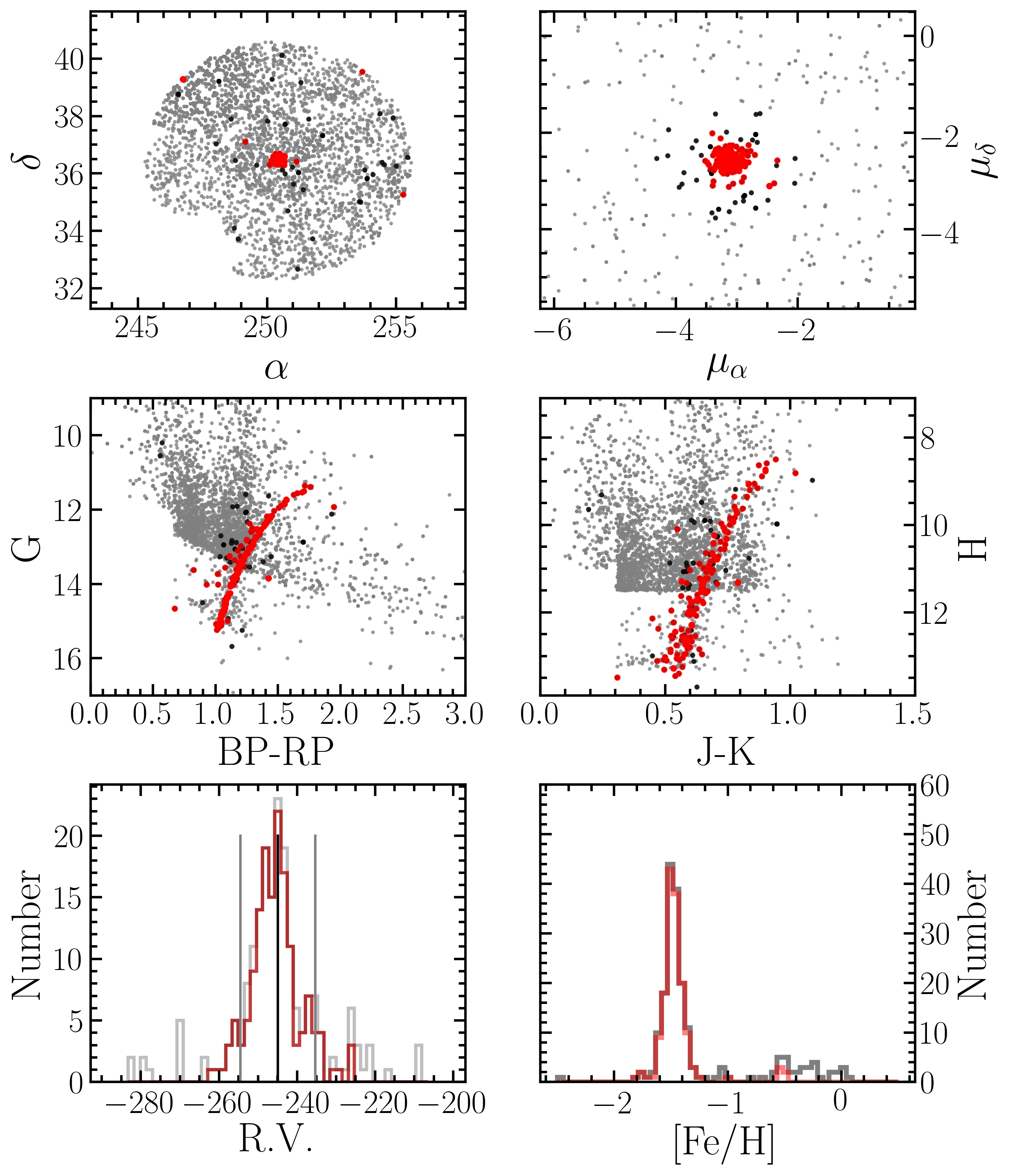
Figure 2: Selecting M13 members in the APOGEE catalogue. In all panels, grey dots represent catalogue stars within 4 r_J of the GC centre. Black dots represent stars whose proper motions differ from the mean value from the VB catalogue by no more than 4 $\sigma_{\rm PV}$. Red dots represent a sub-sample of the former whose radial velocities differ from the GC mean by no more than 3 $\sigma_{\rm RV}$.

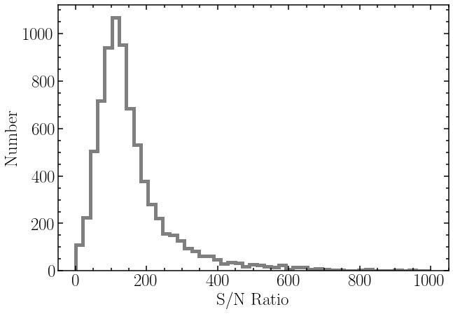
Figure 3: Distribution of the S/N/pixel of the resulting sample.

The situation mandates a strategy based on a sweeping search of the entire APOGEE DR17 catalogue for GC members defined according to a set of homogeneous membership criteria. By proceeding in this way we hope to generate a catalogue that confirms previously established memberships while further extending member samples on the basis of good quality radial velocities and proper motions.

The philosophy underlying our approach is to generously consider every star with a reasonable probability of belonging to a given GC, providing elements to enable the catalogue users to make their own informed sample selections. In short, catalogue completeness is prioritised over purity. Nevertheless, the catalogue is devised in such a way as to make a conservative selection leading up to a very pure sample quite straightforward.

Stars are selected on the basis of angular distance from GC centre, proper motion (PM), and radial velocity (RV) only. Criteria for selection are defined in terms of the GC’s Jacobi radius ($r_{\rm J}$), as well as central values and dispersion of PMs ($\mu_{\rm PM}$ and $\sigma_{\rm PM}$) and RVs ($\mu_{\rm RV}$ and $\sigma_{\rm RV}$). We decided not to use position in the colour-magnitude diagram as a selection criterion, to avoid biasing against possible minority populations. We adopt the following sets of criteria to define two broad types of candidate members:

• Likely members are those meeting a strict set of angular distance, PM, and RV criteria, regardless of their chemical compositions.

• Outliers are stars meeting more relaxed angular distance, PM, and RV criteria, whose metallicities match closely those of nearby GCs.

The Likely group, as its name indicates, contains the stars that have the highest probability of being cluster members. By not imposing a metallicity condition to define this group we wish to avoid missing members for which ASPCAP could not find a metallicity solution (the case of very warm stars) or those with potentially large errors in metallicity, (the case of both very warm and very cool stars or those with low S/N spectra). Moreover, Likely members with very discrepant metallicities could represent a fringe GC population. Conversely, the Outlier group contains stars whose chemical compositions are consistent with membership, but whose position and kinematics suggest at best a loose association. Inclusion of the Outlier group aims at catching a maximum number of extra-tidal stars. In cases of GCs presenting a large spread in metallicity, such as $\omega$ Cen, M 54, Terzan 5, or Liller 1, similarity in terms of [Fe/H] cannot be used to define Outliers, although those with abundance patterns consistent with a second-generation nature are retained and flagged.

The quantitative definitions of these two sub-groups is provided in Table 2. GC centre coordinates, as well as the values for $r_{\rm J}$, $\mu_{\rm PM}$, $\mu_{\rm RV}$, and $\sigma_{\rm RV}$ were adopted from the VB catalogue. The generous upper angular distance limits adopted for Outliers is aimed at enabling the identification of extra-tidal GC members. The method to estimate $\sigma_{\rm PM}$ is described below. The very generous PM threshold was adopted after we found out that some good candidates were located several $\sigma_{\rm PM}$ off of the mean PM value, which may reflect our admittedly rough estimated of $\sigma_{\rm PM}$.

Our procedure can be summarised as follows. We start by obtaining an estimate of the proper motion dispersion, $\sigma_{\rm PM}$. Data from the Gaia eDR3 archive were downloaded for each cluster. Adopting mean proper-motion values from the VB catalogue we calculated $\sigma_{\rm PM}$ through a single $\sigma$-clipping iteration aimed at removing background contamination. That measured dispersion is obviously larger than the intrinsic dispersion, since it folds in measurement errors which are not the same for every cluster. Given those estimates, stars are considered to be Likely GC members if they meet the set of strict criteria listed on the first row of Table 2. Next the APOGEE catalogue was searched for Outliers, by following the set of loose criteria listed on the second row of Table 2. The selection process is illustrated in Figure 2.

The resulting sample consists of a total of 7,737 entries for 6,424 unique candidate members associated with 72 GCs. Multiple entries occur for a number of stars located in overlapping fields and/or observed as part of different programs. The quality of the data is illustrated in Figure 3, which shows the distribution of the median S/N/pixel of the resulting sample, where $\sim$93% of the spectra have S/N$>$50. The distributions of the stars in the Kiel diagram and Gaia colour-magnitude diagram are shown in 4. The right panel of shows the distribution of the sample stars in the Gaia undereddened colour-magnitude diagram, where the range of GC metallicities can be immediately appreciated. In the left panel, sample stars are displayed in the Kiel diagram, which brings to sharp relief the high precision of APOGEE stellar parameters.

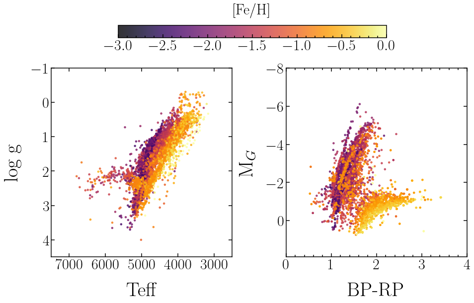
Figure 4: Right: Kiel Diagram for the resulting sample. Note that this plot does not display all stars included in the catalog, as ASPCAP failed to deliver stellar parameters for some stars. Left: Gaia eDR3 CMD of the GC parent sample, including only stars with A${}_{\rm K}<0.3$. In both panels stars are colour-coded by the APOGEE DR17 Fe abundances.

4 Membership Probabilities

In order to provide users of this catalogue with the elements required for deciding which samples should be considered for their analysis, two sets of membership probabilities are provided. The first set is based on a Gaussian mixture modelling of the Gaia eDR3 positions and proper motions of GC stars, and directly imported from the VB catalogue (Section 4.1). In addition, we derive our own set of independent membership probabilities, based on the APOGEE radial velocities.

4.1 Vasiliev & Baumgardt probabilities

For the user’s convenience we briefly summarise the membership probability estimates provided in the VB catalogue. For further details the user is referred to the original papers (Vasiliev & Baumgardt, 2021; Baumgardt & Vasiliev, 2021). Membership probabilities were determined via a mixture modelling approach from which they also infer cluster properties such as mean parallax, proper motion, dispersion and structural parameters. The initial sample is obtained by extracting all sources with 5- or 6-parameter astrometric solutions from Gaia within a certain distance from the centre of each GC, which in the general case is taken to be a few times greater than the cluster half-light radius. A first run of mixture modelling in the 3D astrometric space is performed on a subset of the sources with the most reliable astrometry, where one of the Gaussian components represents the cluster and the remaining component(s) account for the field stars. A full mixture model is then run, where a Plummer model is adopted to match each GC’s density profile, with the scale radius as a free parameter. The parameter space is explored with a Markov Chain Monte Carlo code initialised with astrometric parameters determined by extreme deconvolution. Membership probabilities for each star are then determined following convergence of the MCMC runs. Colour-magnitude diagrams of members thus obtained for each GC are inspected visually to verify the outcome of the mixture model, which did not utilise any the photometric information. Finally, the mean parallax and proper motion of each cluster and their uncertainties are taken from the MCMC chain.

4.2 RV-based Probabilities

Exceedingly accurate radial velocities are one of the main data products of the APOGEE survey. This can be verified through a quick comparison with the data from latest Gaia release (DR3, Gaia Collaboration et al., 2022). We cross-matched our sample for M 13 with the Gaia DR3 catalogue, obtaining 108 matches. The mean heliocentric radial velocity and r.m.s. scatter for each sample are in excellent agreement, with ${\rm<rv_{APO}>}=-246.30~{}{\rm km~{}s}^{-1}$ and ${\rm<\sigma_{APO}>}=5.27~{}{\rm km~{}s}^{-1}$ for the APOGEE sample, and ${\rm<rv_{Gaia}>}=-246.33~{}{\rm km~{}s}^{-1}$ and ${\rm<\sigma_{Gaia}>}=5.95~{}{\rm km~{}s}^{-1}$. It is noteworthy that the mean radial velocities agree to within 30 ${\rm m~{}s^{-1}}$, reflecting the great accuracy of the two data sets. In addition, the r.m.s. scatter, which results from the convolution between the cluster velocity dispersion and measurement error, is lower in the APOGEE sample by $\sim$12%, reflecting APOGEE’s superior radial velocity precision.

We take advantage of this high-quality data set to complement the membership information available from the VB catalogue with RV based membership probabilities. These probabilities were estimated as follows. We adopted a procedure similar to that of Gieseking (1985) whereby the RV distribution within the field of each GC was modelled as a combination of Gaussian functions plus a constant background. For any given star $i$, the RV-based membership probability is given by:

$$p_{i}={\rm\frac{G_{\rm gc}(v_{i})}{G_{\rm gc}(v_{i})+B(v_{i})}}$$ (1)

Where ${\rm v_{i}}$ is the radial velocity of the star, ${\rm G_{gc}(v)}$ is the Gaussian function describing the RV distribution of the GC, and ${\rm B(v)}$ is a function accounting for the RV distribution of the field background.

For well-sampled GCs, the functions ${\rm G_{gc}(v)}$ and ${\rm B(v)}$ were obtained from a fit to the RV distribution from the stars contained within the field of each GC. In cases where the GC is poorly sampled and/or the contrast with the background is poor, the ${\rm G_{gc}(v)}$ function adopted was based on parameters (mean RV and velocity dispersion) gathered from the VB catalogue. The background function ${\rm B(v)}$, in the general case, was a combination of Gaussians and a constant floor value. In no case were more than two Gaussians required to account for the background data. An example fit is shown in Figure 5.

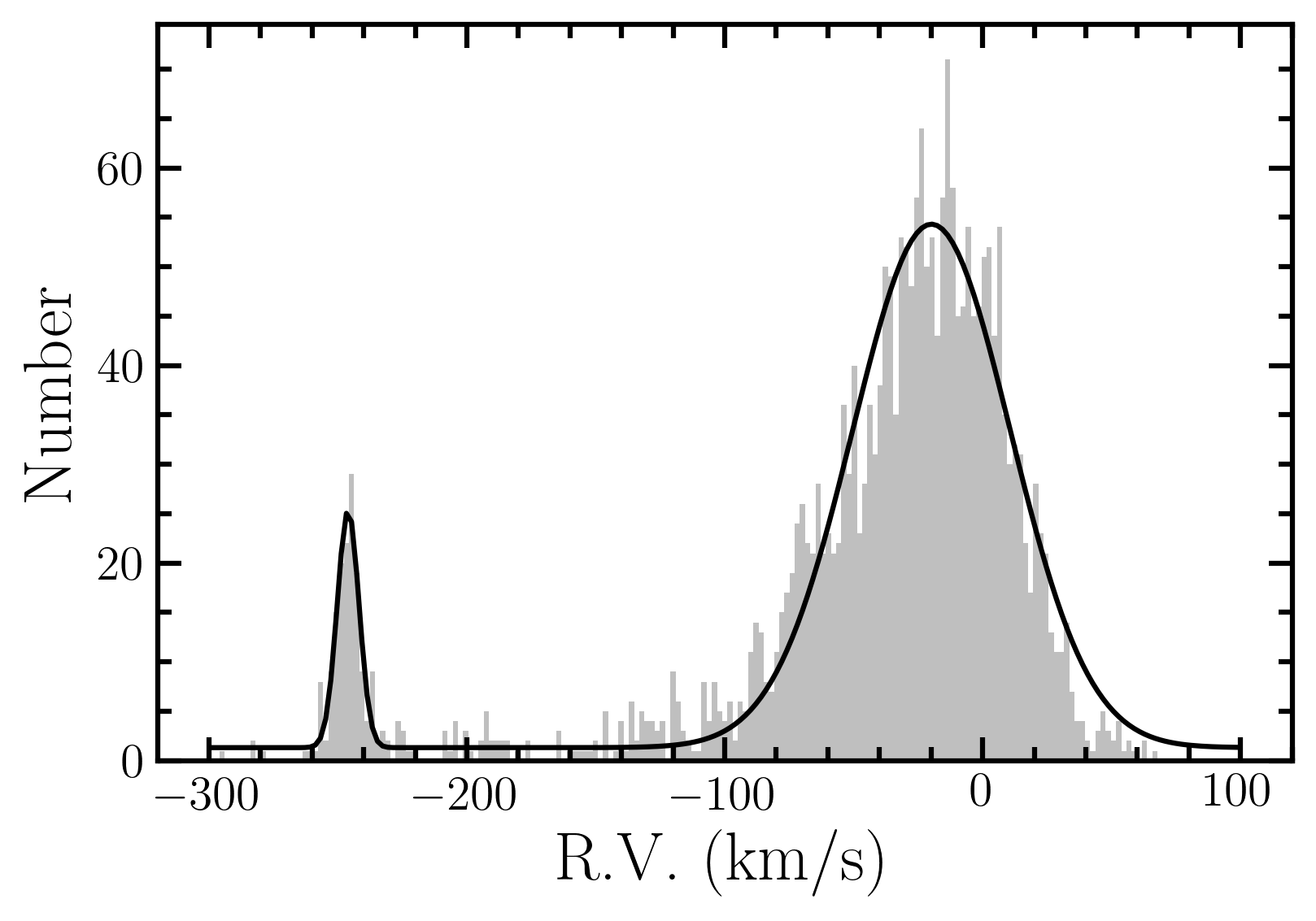
Figure 5: Fit of the RV distribution in the field of M13. The model fit is a double Gaussian with an additional constant background. The secondary peak corresponds to the RVs of the cluster.

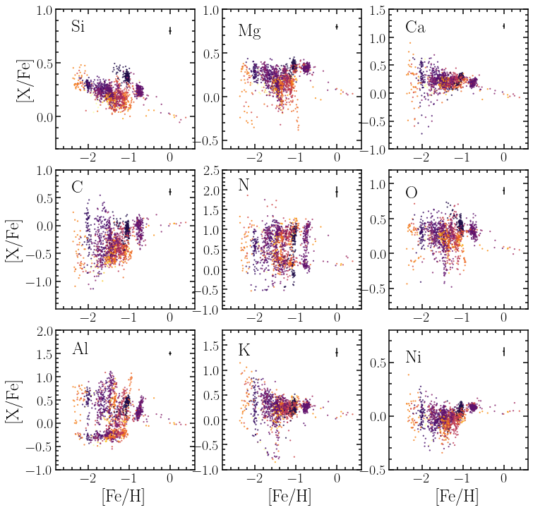
Figure 6: Sample elemental abundances for Galactic GCs included in the VAC. Only abundances derived from spectra with S/N$>$150 are shown. To distinguish individual GCs, data are colour-coded by the cluster heliocentric distance. GCs with large spreads in metallicity, namely $\omega$ Cen and M 54, are excluded from this plot. Mean error bars are displayed on the top right of each panel.

5 Results and Science Highlights

This value-added catalogue can be employed in a myriad of different science projects. We highlight a few aspects of the data base that illustrate its potential. In Figure 6, selected elemental abundances sampling different nucleosynthetic pathways are displayed in various panels. Only abundances derived from spectra with S/N$>$150 are shown. To distinguish stars associated with individual GCs, symbols are colour-coded by heliocentric distance. The complexity of the GC member candidates distribution in chemical-composition space is promptly evident from a first glance to these data.

In Figure 7, the data for M 5 (NGC 5904) are displayed on the [C/Fe] vs [N/Fe] plane, where symbols are colour-coded by surface gravity ($\log g$). Two sequences are clearly visible, where a gentle variation of N and C abundances can be seen to be correlated with $\log g$. This variation is due to mixing along the giant branch, whereby more evolved stars (lower $\log g$) display depleted C and enhanced N due to the progressive mixing of CNO-processed material during the evolution along the red giant branch. The more drastic variation associated with the MP phenomenon connects stars with same $\log g$ between the two sequences (e.g., Phillips et al., 2022).

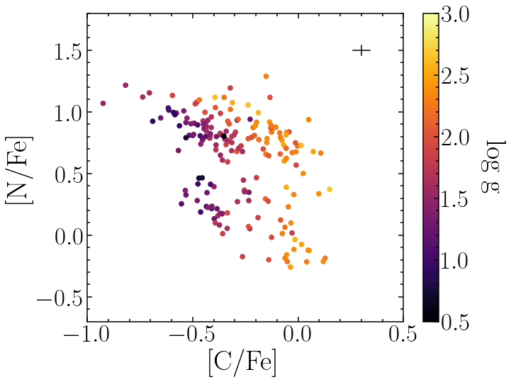
Figure 7: Carbon-Nitrogen anti-correlation in the globular cluster M5 (NGC 5904). Symbols are colour-coded by surface gravity ($\log g$) to distinguish C-N abundance variations due to stellar evolution from those associated with the multiple populations phenomenon. Two diagonal sequences can be seen. Along each sequence, the variations of N and C abundances are correlated with $\log g$, as deep mixing brings the byproducts of the CNO-cycle to the star’s surface steadily changing its chemical composition during evolution along the giant branch. The more drastic anti-correlation due to the MP phenomenon connects stars with same $\log g$ between the two sequences. Mean error bars are displayed on the top right.

In Figure 8, data for various GCs with [Fe/H]$<-0.5$ are displayed on the [Mg/Fe] vs [Al/Fe] plane. Symbols are colour-coded by metallicity. Metal-poor GCs show a strong anti-correlation between these two elements. The various GC sequences are displaced relative to each other due to variations in the systems’ natal chemical compositions, associated with their origin. The weakening of this anti-correlation with increasing metallicity (e.g., Nataf et al., 2019) manifests itself by the near absence of an anti-correlation in the most metal-rich GCs.

Finally, in the Appendix we present a comparison of the APOGEE DR17 elemental abundances published in this value added catalogue with data from various sources from the literature.

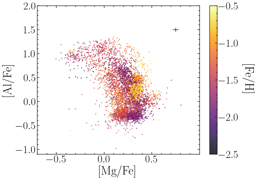
Figure 8: Magnesium-Aluminium anti-correlation for a collection of GCs with [Fe/H]$\leq-0.5$. Different sequences are displaced on this plane according to GC natal chemical composition. The Mg-Al anti-correlation is weakened or even absent towards higher metallicity. Mean error bars are displayed on the top right.

5.1 Extra-tidal candidates

Globular clusters are slowly dissolving, shedding stars under the combined effect of evaporation and tidal stripping as they follow their orbits within the Milky Way dark matter halo. Evidence to this phenomenon has been documented as stars are detected beyond GC tidal radii, in the form of tidal streams (e.g., Odenkirchen et al., 2001; Belokurov et al., 2006; Grillmair & Johnson, 2006; Bonaca & Hogg, 2018; Malhan et al., 2021) and diffuse outer envelopes or less defined collections of extra-tidal stars (e.g., Kuzma et al., 2016; Kuzma et al., 2018; Chun et al., 2020; Kundu et al., 2022; Piatti, 2022).

Identifying extra-tidal stars is a difficult task requiring deep photometry over a wide field of view. More recently, data from the Gaia satellite have enabled the use of proper motions for that purpose (e.g., Kundu et al., 2019). In the past decade, chemical tagging has been used to identify field stars with chemistry that is characteristic of GC populations (e.g., Martell & Grebel, 2010; Lind et al., 2015; Martell et al., 2016; Schiavon et al., 2017a; Fernández-Trincado et al., 2017; Tang et al., 2019), leading up to moderately robust estimates of the contribution of dissolved GCs to the Milky Way stellar halo mass budget (e.g., Martell et al., 2011; Schiavon et al., 2017a; Koch et al., 2019; Horta et al., 2021).

Linking so-called “N-rich” field stars with their parent GCs is quite important as a means to establish once and for all their GC origin (e.g., Kisku et al., 2021). However, such associations have proved difficult, resulting from likelihood estimates based on orbital parameters (e.g., Savino & Posti, 2019).

Detailed chemistry and precision radial velocities for large samples, combined with Gaia-quality astrometry and GC structural parameters can make an important contribution in this context. Large samples with precision chemistry enables unequivocal association of extra-tidal stars with their parent GCs. Indeed, recent work has provided evidence for the presence of N-rich stars beyond the Jacobi radius of M 54 and Palomar 5 (Fernández-Trincado et al., 2021a; Phillips et al., 2022).

In Figure 9 VAC data are displayed on various chemical planes. Data for the $\omega$ Cen and M 54 are omitted from these plots. Grey dots show the whole sample, and black dots represent only stars located beyond the Jacobi radius of their parent GC. While most extra-tidal stars have normal chemistry, a few dozen N-rich stars can be identified in those planes, due to their enhanced abundances of N and Al, and depleted Mg and O. Extra-tidal stars can be easily identified in the VAC by the value of the parameter DPOS, which is equal to the angular distance to each GC centre, in units of $r_{J}$. Extra-tidal stars have DPOS > 1.

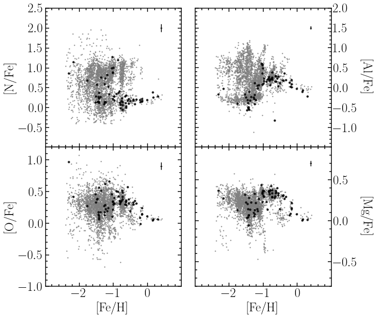
Figure 9: Candidate GC members in various chemical planes. Stars within their parent GC Jacobi radii are shown as grey symbols whereas extra-tidal stars are displayed as black dots. A substantial fraction of the extra-tidal stars have N-rich abundance patterns, confirming the GC-origin of N-rich stars identified in previous studies. For previous identifications of extra-tidal N-rich stars see discussion in text. Mean error bars are displayed on the top right of each panel.

5.1.1 The case of M 54

M 54 is the nuclear cluster of the Sagittarius dwarf Spheroidal (Sgr dSph). Its chemodynamical properties have been studied extensively (e.g., Law & Majewski, 2010; Mucciarelli et al., 2017) and merit some attention. In Figure 10 we show the data for M 54 members on the same chemical planes as Figure 9. Top/bottom panels show intra/extra-tidal stars. It is noteworthy that this cluster is characterised by a very large population of extra-tidal stars, some of which have N-rich abundance patterns (see, e.g., Fernández-Trincado et al., 2021a). Indeed, a large fraction of the entire population of extra-tidal stars identified in this work are associated with M 54. That could be a result of the cluster’s undergoing severe tidal disruption under the MW potential, or rather reflect a possible underestimate of the M 54’s Jacobi radius. Such estimates are plagued by considerable uncertainties. In the case of M 54, the situation is made worse by the fact that it is not known whether the cluster is positioned at the centre of its host galaxy’s potential well, and whether it possesses its own dark matter halo (e.g., Carlberg & Grillmair, 2022). In view of these uncertainties, we decide to retain a large number of M 54 candidate members, while acknowledging the reality that this sample is considerably contaminated by Sgr dSph field stars. The catalogue users are again provided with data they can use to select sub-samples according to their science goals.

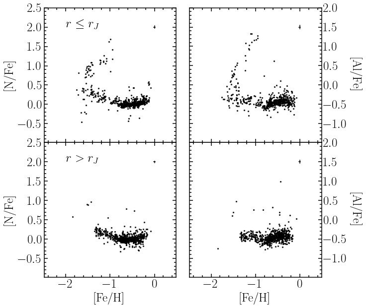
Figure 10: Candidate members of M 54 (NGC 6715), the nuclear cluster of the Sagittarius dwarf spheroidal, on the N-Fe and Al-Fe chemical planes. Stars located within (top panel) or beyond (bottom) the cluster’s Jacoby radius are displayed. Note the large number of extra-tidal N-rich and/or Al-rich stars (bottom panel). It is not clear whether this effect is real or due to an underestimate of M 54’s Jacobi radius. Mean error bars are displayed on the top right of each panel.

5.2 Abundance spreads and global parameters

As discussed in the Introduction, perhaps the most puzzling observational feature of GCs is the presence of large anti-correlated spreads of the abundances of light elements. Despite many efforts from various groups, no particular scenario has been able to account for this phenomenon in a quantitative fashion (see review by Bastian & Lardo, 2018). Naturally, correlations between chemical-composition spreads and GC global parameters can provide valuable constraints on formation models. In this Section we provide a brief foray into the topic, exploring how this new catalogue can potentially contribute to this discussion. We focus on Al spreads. Aluminium abundances are exceptionally well-measured in APOGEE spectra, over a wide range of metallicities. Moreover, unlike nitrogen, aluminium spreads can be assessed in a fairly unambiguous way, since the abundance of this element is not affected by stellar evolution effects.

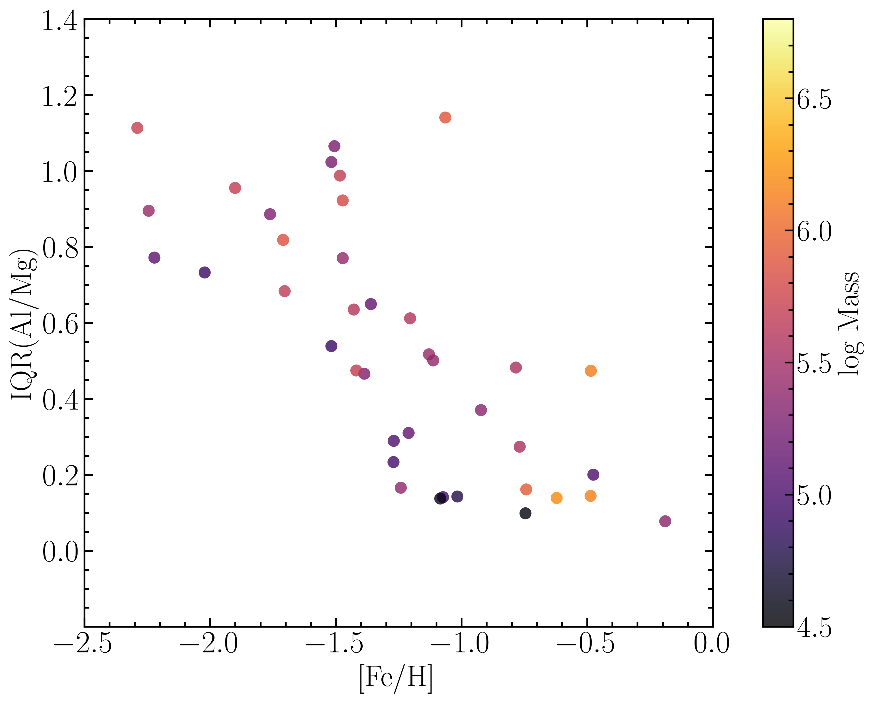
Figure 11: Inter-quartile range of the [Al/Mg] ratio plotted against GC metallicity. A remarkable anti-correlation between the two quantities is apparent, with high significance ($\rho_{x}=-0.76$). Symbols are colour-coded by log GC mass, but no correlation is apparent.

Following Carretta et al. (2010), who adopted the [O/Na] inter-quartile range as a measure of abundance spreads, we measure the inter-quartile range of the [Al/Mg] ratio. We first examine the well known anti-correlation of aluminium spreads with GC metallicity (see also Nataf et al., 2019; Mészáros et al., 2020). The data are displayed in Figure 11, where a very clear anti-correlation between IQR(Al/Mg) and [Fe/H] is present, with a Spearman Rank correlation coefficient $\rho_{x}=-0.76$. This result confirms previous studies reporting a substantial decrease of Al spreads in high-metallicity GCs. Symbols are colour-coded by GC mass, but no clear correlation with that parameter can be seen.

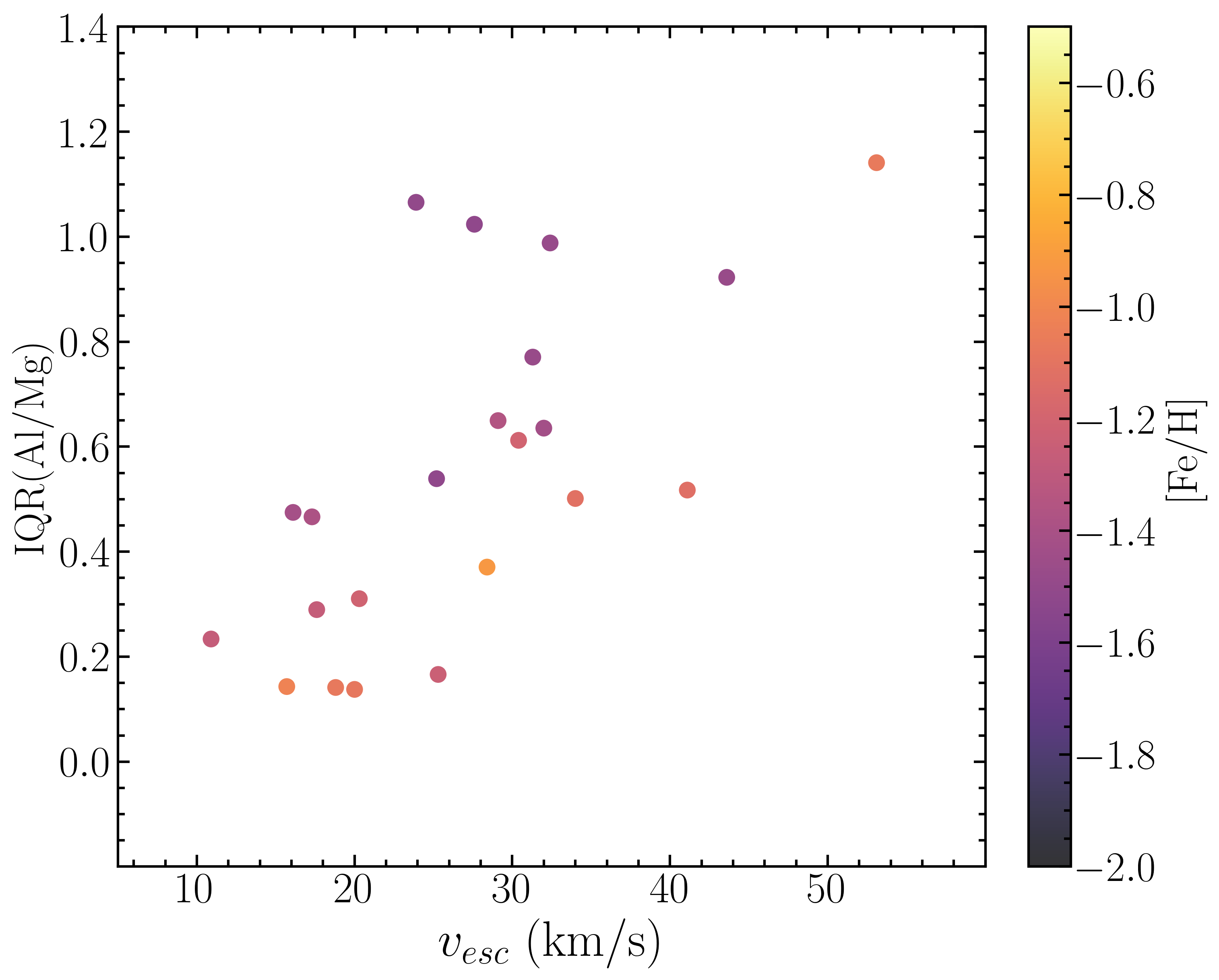
Figure 12: Inter-quartile range of the [Al/Mg] ratio plotted against central escape velocity. A strong correlation is present ($\rho_{x}=0.68)$, but only after controlling for the effect of metallicity. Only GCs with –1.7<[Fe/H]<–0.8 are considered. Symbols are colour-coded by [Fe/H]. This might be an indicator of chemical enrichment due to a history of feedback-regulated star formation.

.

Next, we examine the presence of a correlation between abundance spreads and a quantity related to a GC’s gravitational potential. Such a correlation is interesting, as it may be an indication of the presence of chemical enrichment brought about by a history of feedback-regulated star formation (see also Carretta et al., 2010; Schiavon et al., 2013; Sakari et al., 2016). In Figure 12, we plot IQR(Al/Mg) against central escape velocity, from the VB catalogue. Because the correlation between IQR(Al/Mg) and metallicity is so strong, we must control for this parameter, so only GCs with –1.7<[Fe/H]<–0.8 are shown. A strong correlation is seen ($\rho_{x}=0.68$). We also find a strong correlation with central velocity dispersion ($\rho_{x}=0.69$) and GC mass ($\rho_{x}=0.62$).

Figure 13: Inter-quartile range of the [Al/Mg] ratio plotted against a horizontal-branch morphology parameter, $\Delta$(V–I), which is higher for bluer horizontal-branch morphologies. A fairly strong correlation is present ($\rho_{x}=0.63)$, in the sense that only GCs with high IQR(Al/Mg) present a blue HB. Although GCs with red HBs can also have high IQR(Al/Mg), all GCs with low IQR(Al/Mg) have red HBs.

.

We conclude by inspecting the relation between abundance spread and horizontal-branch (HB) morphology. A correlation between these observatbles is expected because the morphology of the HB is in part dictated by the abundance of helium, an element for which there is strong evidence for abundance spreads (e.g., Renzini, 2008). In the following, we adopt IQR(Al/Mg) as a surrogate for a spread in the abundance of helium. The data are displayed in Figure 13, where IQR(Al/Mg) is plotted against the $\Delta$(V–I) parameter from Dotter et al. (2010). High values of $\Delta$(V–I) correspond to blue HB morphology. Although we find a relatively high Spearman rank correlation coefficient ($\rho_{x}=0.63$), the data behave in a subtle way. There is a zone of avoidance at low IQR(Al/Fe) and blue HB morphology. GCs with large abundance spreads can have either a red or a blue HB, but those with low spreads are all characterised by a red HB. This may be related to the fact that the morphology of the horizontal branch is affected by a number of parameters besides He abundance, including age, binarity, and mass loss during the first-ascent red giant-branch phase.

6 The Catalogue

The value-added catalogue presented in this paper consists of two files in FITS format. The catalogue itself is contained in file VAC_GC_DR17_synspec_rev1.fits, which includes all the data from the APOGEE DR17 allStar-dr17-synspec_rev1.fits for each of the 7,737 entries associated with GC candidate members. This file also incorporates distances from GC centres (in units of $r_{\rm J}$), residual proper motions, radial velocities, and [Fe/H], in units of the r.m.s. dispersions of those values. Two sets of membership probabilities are also provided, those based on the radial velocity analysis in Section 4.2 and those from the VB catalogue, when available. Another file, named GC_parameters_VAC.fits contains, for each GC, the mean and r.m.s. values for RVs, proper motions, and metallicities, as well as a number of global parameters from the literature. Both files are available for download from the SDSS DR17 value added catalog webpage (https://www.sdss4.org/dr17/data_access/value-addedcatalogs/).

Data availability

All data used in this paper are publicly available at the SDSS-IV DR17 website: https: /www.sdss.org/dr17/.

Appendix A Comparison with data from the literature

Elemental abundance analysis is a tricky procedure with outputs that depend strongly on a number of factors. On the empirical side, the results are sensitive to the choice of spectral region as well as the overall quality of the observational data, usually quantified in terms of S/N, resolution, and sampling. In addition, the adequacy of data reduction methods is critical, with details such as sky subtraction and telluric absorption elimination being particularly relevant in the NIR. The outcome is also strongly influenced by the arsenal employed in the analysis, including model atmospheres, line opacities (wavelengths, molecular and atomic excitation/ionization potentials, log gfs, damping constants), spectrum synthesis code, microturbulent velocities, and assumptions such as spherical symmetry versus plane parallel atmospheres, and consideration or not of local thermodynamic equilibrium. In modern times, the advent of massive surveys brought to the fore the automation of the core of the spectral analysis, introducing additional uncertainties. It is thus par for the course that the fidelity of any new data set be scrutinised via comparison with numbers generated independently.

APOGEE data have been regularly contrasted with literature values. The survey was indeed designed so as to afford such detailed comparisons, which were performed for each successive data release, and published in a number of papers (e.g., Holtzman et al., 2015; Mészáros et al., 2015; Holtzman et al., 2018; Nataf et al., 2019; Jönsson et al., 2018, 2020; Mészáros et al., 2020, 2021). To our knowledge however, such a detailed examination of DR17 data has not yet been published, particularly within the regime of globular clusters, whose stars inhabit unique loci of chemical composition space. We briefly examine in this Appendix a few comparisons with data from a large survey and those from other smaller independent studies.

Figure 14: Comparison between elemental abundances for stars in common between APOGEE and GALAH surveys, colour-coded by [Fe/H]. The solid horizontal lines indicate identical abundances, whereas the dashed gray lines mark the position of the mean residuals. For all elements, except for oxygen, the mean residuals are much smaller than the r.m.s. of the distribution.

We start by comparing our numbers with those generated by the GALAH survey (De Silva et al., 2015; Martell et al., 2017). For that purpose, we matched our sample stars with the GALAH DR3 catalogue (Buder et al., 2022), retaining only the elemental abundances with quality flag=0, which yielded several hundred stars in common for all abundances of interest. The comparisons are displayed in Figure 14, and the relevant statistics listed in Table 3. Perfect agreement is indicated by the solid black line, whereas the mean difference is marked by the gray dashed line. Mean residuals and r.m.s. dispersion are indicated on the top right of each panel. Data points are colour-coded by [Fe/H]. For all abundances the mean residuals are well within the r.m.s., except for the case of oxygen, for which the mean residuals are just above 1 $\sigma$ off. It is also noteworthy that for some elements, such as O, K, Cr, V, and Ce the dispersion of the abundance ratio residuals is particularly large.

By looking at the intrinsic dispersion of the abundance ratios in the two data sets, we can pinpoint which of them contributes more importantly to the scatter in the data. Columns (3) and (4) of Table 3 display the numbers, obtained by simply calculating the r.m.s. of the abundances from APOGEE and GALAH, using only the stars in common for a fair assessment. For Mg, Si, O, and Ni the intrinsic scatter in the GALAH data is up to twice larger than APOGEE. The opposite is the case for Cr and, to some extent, Ce. For all the other elements, including those for which a large intrinsic scatter renders the comparison somewhat difficult to interpret (Fe and Al), the two sets have comparable dispersion. We conclude that for most elements involved in this comparison, the precision of the APOGEE data is superior to that of GALAH, within this restricted data set. By the same token, for all elements except oxygen, the zero points of the two abundance systems are indistinguishable from each other.

Table 3: Comparison of abundances from APOGEE and GALAH. Column information: (1) Iron abundance or abundance ratio; (2) Mean residual and r.m.s. dispersion around the mean; (3) Intrinsic r.m.s. of APOGEE data; (4) Intrinsic r.m.s. of GALAH data; (5) Number of stars in common.

Abundance	Residual	$\sigma_{APO}$	$\sigma_{GAL}$	n⋆
(1)	(2)	(3)	(4)	(5)
$\lceil{\rm Fe/H}\rceil$	$-0.08\pm 0.15$	0.44	0.44	447
$\lceil{\rm Mg/Fe}\rceil$	$0.07\pm 0.16$	0.14	0.21	423
$\lceil{\rm Si/Fe}\rceil$	$0.00\pm 0.13$	0.07	0.13	441
$\lceil{\rm Ca/Fe}\rceil$	$-0.06\pm 0.21$	0.16	0.17	417
$\lceil{\rm O/Fe}\rceil$	$-0.38\pm 0.31$	0.15	0.33	317
$\lceil{\rm Al/Fe}\rceil$	$-0.06\pm 0.25$	0.33	0.33	294
$\lceil{\rm K/Fe}\rceil$	$0.11\pm 0.35$	0.25	0.25	395
$\lceil{\rm Ni/Fe}\rceil$	$0.07\pm 0.16$	0.09	0.15	398
$\lceil{\rm Mn/Fe}\rceil$	$0.00\pm 0.24$	0.20	0.18	365
$\lceil{\rm Cr/Fe}\rceil$	$0.09\pm 0.37$	0.33	0.19	380
$\lceil{\rm V/Fe}\rceil$	$-0.12\pm 0.45$	0.27	0.35	188
$\lceil{\rm Ce/Fe}\rceil$	$0.00\pm 0.24$	0.40	0.33	165

Figure 15: Comparison of APOGEE abundances for O (top panel) and Fe with values obtained by E. Carretta and collaborators (middle panel for abundances obtained from neutral lines, bottom panel for those based on once-ionised iron). Good agreements is achieved for [O/Fe], but for [Fe/H] the mean residuals are off at the 1 $\sigma$ level. There is also evidence for a dependence of residuals on metallicity.

Figure 16: Comparison of APOGEE abundances for other elements with values other sources in the literature. We find excellent agreement for most elements, and satisfactory agreement for Al and N, with no obvious dependence on metallicity or $T_{\rm eff}$ (except perhaps for N).

To address the matter of data accuracy, we need to resort to comparisons with other literature values based on classical abundance analysis of high-resolution (predominantly optical) spectra. The best place to start is the extensive data set painstakingly amassed over the years by E. Carretta and collaborators. The compilation presented by Carretta et al. (2010) focuses on Fe, O, and Na, but we limit our discussion to the former two elements. APOGEE abundances for Na are known to suffer from important shortcomings in the metallicity regime of interest, as they are based on only two lines that are weak in the spectra of metal-poor giants. Moreover, they are affected by important contamination by airglow emission (Jönsson et al., 2020).

Stars in common to this value-added catalogue and Carretta et al. (2010) are displayed in abundance residuals vs. $T_{\rm eff}$ planes in Figure 15. The top panel compares APOGEE vs Carretta et al. (2010) values for [O/Fe], whereas comparisons of Fe abundances derived using lines due to neutral and once-ionized iron are displayed in the middle and bottom panels, respectively. Non-negligible differences, at the 1 $\sigma$ level, are seen between the two sets of Fe abundances. A mild dependence on metallicity is apparent, with good agreement on the high metallicity end, and a slight deterioration at [Fe/H]$\mathrel{\hbox{\raise 2.15277pt\hbox{$<$}\hbox to0.0pt{\hss\lower 2.15277pt\hbox{$\sim$}}}}$–1.0. Overall, we conclude that the agreement between the Fe abundances of APOGEE and Carretta et al. (2010) is about satisfactory. Regarding oxygen abundances, the mean difference between the two sets is $\sim$0.1 dex, which is well within the r.m.s. scatter, suggesting that the discrepancy between APOGEE and GALAH on the same plane (Figure 14) is due to systematics in the GALAH data.

We wrap up our verification of APOGEE abundances against the literature by extending our scrutiny to additional elements. Figure 16 contrast APOGEE abundances with data from a variety of literature sources, originally compiled by Mészáros et al. (2015). Abundances shown are those for C, N, O, Ca, Si, and Al. For all elements, the mean residuals are consistent with with the identity line well within the r.m.s. dispersion. For N and Al the scatter is larger, and in the case of the former there seems to be a dependence on metallicity. This is perhaps not surprising, because APOGEE N abundances rely on CN lines, which become vanishingly weak in giant stars with [Fe/H]$\mathrel{\hbox{\raise 2.15277pt\hbox{$<$}\hbox to0.0pt{\hss\lower 2.15277pt\hbox{$\sim$}}}}$–2.0. Outside that regime, agreement between APOGEE and the literature sources is actually very good.

In conclusion, comparison between APOGEE chemical compositions and data from GALAH and a compilation of classical abundance analyses from the literature indicates that APOGEE chemistry for Galactic globular cluster members is characterised by excellent precision and very good accuracy.

References

- Abdurro’uf et al. (2022) Abdurro’uf et al., 2022, ApJS, 259, 35
- Allende Prieto et al. (2006) Allende Prieto C., Beers T. C., Wilhelm R., Newberg H. J., Rockosi C. M., Yanny B., Lee Y. S., 2006, ApJ, 636, 804
- Armandroff & Zinn (1988) Armandroff T. E., Zinn R., 1988, AJ, 96, 92
- Ashman & Zepf (1992) Ashman K. M., Zepf S. E., 1992, ApJ, 384, 50
- Astropy Collaboration et al. (2013) Astropy Collaboration et al., 2013, aap, 558, A33
- Barbuy et al. (1998) Barbuy B., Bica E., Ortolani S., 1998, A&A, 333, 117
- Bastian & Lardo (2018) Bastian N., Lardo C., 2018, ARA&A, 56, 83
- Baumgardt & Vasiliev (2021) Baumgardt H., Vasiliev E., 2021, MNRAS, 505, 5957
- Beaton et al. (2021) Beaton R. L., et al., 2021, AJ, 162, 302
- Bekki & Freeman (2003) Bekki K., Freeman K. C., 2003, MNRAS, 346, L11
- Belokurov et al. (2006) Belokurov V., Evans N. W., Irwin M. J., Hewett P. C., Wilkinson M. I., 2006, ApJ, 637, L29
- Belokurov et al. (2018) Belokurov V., Erkal D., Evans N. W., Koposov S. E., Deason A. J., 2018, MNRAS, 478, 611
- Bica & Alloin (1986) Bica E., Alloin D., 1986, A&A, 162, 21
- Blanton et al. (2017) Blanton M. R., et al., 2017, AJ, 154, 28
- Bolte & Hogan (1995) Bolte M., Hogan C. J., 1995, Nature, 376, 399
- Bonaca & Hogg (2018) Bonaca A., Hogg D. W., 2018, ApJ, 867, 101
- Bovy (2015) Bovy J., 2015, ApJS, 216, 29
- Bowen & Vaughan (1973) Bowen I. S., Vaughan A. H. J., 1973, Appl. Opt., 12, 1430
- Briley et al. (1997) Briley M. M., Smith V. V., King J., Lambert D. L., 1997, AJ, 113, 306
- Brodie & Strader (2006) Brodie J. P., Strader J., 2006, ARA&A, 44, 193
- Buder et al. (2022) Buder S., et al., 2022, MNRAS, 510, 2407
- Caldwell et al. (2009) Caldwell N., Harding P., Morrison H., Rose J. A., Schiavon R., Kriessler J., 2009, AJ, 137, 94
- Callingham et al. (2022) Callingham T. M., Cautun M., Deason A. J., Frenk C. S., Grand R. J. J., Marinacci F., 2022, MNRAS, 513, 4107
- Cannon et al. (1998) Cannon R. D., Croke B. F. W., Bell R. A., Hesser J. E., Stathakis R. A., 1998, MNRAS, 298, 601
- Carlberg & Grillmair (2022) Carlberg R. G., Grillmair C. J., 2022, ApJ, 935, 14
- Carretta & Gratton (1997) Carretta E., Gratton R. G., 1997, A&AS, 121, 95
- Carretta et al. (2009) Carretta E., Bragaglia A., Gratton R., Lucatello S., 2009, A&A, 505, 139
- Carretta et al. (2010) Carretta E., Bragaglia A., Gratton R. G., Recio-Blanco A., Lucatello S., D’Orazi V., Cassisi S., 2010, A&A, 516, A55
- Castellani & degl’Innocenti (1999) Castellani V., degl’Innocenti S., 1999, A&A, 344, 97
- Cavallo & Nagar (2000) Cavallo R. M., Nagar N. M., 2000, AJ, 120, 1364
- Chiosi et al. (1992) Chiosi C., Bertelli G., Bressan A., 1992, ARA&A, 30, 235
- Choksi et al. (2018) Choksi N., Gnedin O. Y., Li H., 2018, MNRAS, 480, 2343
- Chun et al. (2020) Chun S.-H., Lee J.-J., Lim D., 2020, ApJ, 900, 146
- Cohen & Meléndez (2005) Cohen J. G., Meléndez J., 2005, AJ, 129, 303
- Cohen et al. (2017) Cohen R. E., Moni Bidin C., Mauro F., Bonatto C., Geisler D., 2017, MNRAS, 464, 1874
- Cunha et al. (2017) Cunha K., et al., 2017, ApJ, 844, 145
- De Silva et al. (2015) De Silva G. M., et al., 2015, MNRAS, 449, 2604
- Denissenkov & Weiss (1996) Denissenkov P. A., Weiss A., 1996, A&A, 308, 773
- Dotter et al. (2010) Dotter A., et al., 2010, ApJ, 708, 698
- Fall & Rees (1985) Fall S. M., Rees M. J., 1985, ApJ, 298, 18
- Fernández-Trincado et al. (2017) Fernández-Trincado J. G., et al., 2017, ApJ, 846, L2
- Fernández-Trincado et al. (2021a) Fernández-Trincado J. G., et al., 2021a, A&A, 648, A70
- Fernández-Trincado et al. (2021b) Fernández-Trincado J. G., et al., 2021b, ApJ, 908, L42
- Fernández-Trincado et al. (2022) Fernández-Trincado J. G., Minniti D., Garro E. R., Villanova S., 2022, A&A, 657, A84
- Forbes (2020) Forbes D. A., 2020, MNRAS, 493, 847
- Gaia Collaboration et al. (2021) Gaia Collaboration et al., 2021, A&A, 649, A1
- Gaia Collaboration et al. (2022) Gaia Collaboration et al., 2022, arXiv e-prints, p. arXiv:2208.00211
- Galleti et al. (2007) Galleti S., Bellazzini M., Federici L., Buzzoni A., Fusi Pecci F., 2007, A&A, 471, 127
- García Pérez et al. (2016) García Pérez A. E., et al., 2016, AJ, 151, 144
- Geisler et al. (2021) Geisler D., et al., 2021, A&A, 652, A157
- Gieseking (1985) Gieseking F., 1985, A&AS, 61, 75
- Gratton et al. (2012) Gratton R. G., Carretta E., Bragaglia A., 2012, A&ARv, 20, 50
- Grillmair & Johnson (2006) Grillmair C. J., Johnson R., 2006, ApJ, 639, L17
- Gunn et al. (2006) Gunn J. E., et al., 2006, AJ, 131, 2332
- Gustafsson et al. (2008) Gustafsson B., Edvardsson B., Eriksson K., Jørgensen U. G., Nordlund Å., Plez B., 2008, A&A, 486, 951
- Hasselquist et al. (2016) Hasselquist S., et al., 2016, ApJ, 833, 81
- Helmi et al. (2018) Helmi A., Babusiaux C., Koppelman H. H., Massari D., Veljanoski J., Brown A. G. A., 2018, Nature, 563, 85
- Holtzman et al. (2015) Holtzman J. A., et al., 2015, AJ, 150, 148
- Holtzman et al. (2018) Holtzman J. A., et al., 2018, AJ, 156, 125
- Horta et al. (2020) Horta D., et al., 2020, MNRAS, 493, 3363
- Horta et al. (2021) Horta D., et al., 2021, MNRAS, 500, 5462
- Hubeny & Lanz (2017) Hubeny I., Lanz T., 2017, arXiv e-prints, p. arXiv:1706.01859
- Hunter (2007) Hunter J. D., 2007, Computing In Science & Engineering, 9, 90
- Ivans et al. (2001) Ivans I. I., Kraft R. P., Sneden C., Smith G. H., Rich R. M., Shetrone M., 2001, AJ, 122, 1438
- Johnson & Pilachowski (2010) Johnson C. I., Pilachowski C. A., 2010, ApJ, 722, 1373
- Johnson & Pilachowski (2012) Johnson C. I., Pilachowski C. A., 2012, ApJ, 754, L38
- Johnson et al. (2005) Johnson C. I., Kraft R. P., Pilachowski C. A., Sneden C., Ivans I. I., Benman G., 2005, PASP, 117, 1308
- Jönsson et al. (2018) Jönsson H., et al., 2018, AJ, 156, 126
- Jönsson et al. (2020) Jönsson H., et al., 2020, AJ, 160, 120
- Kamann et al. (2018) Kamann S., et al., 2018, MNRAS, 473, 5591
- Kisku et al. (2021) Kisku S., et al., 2021, MNRAS, 504, 1657
- Koch & McWilliam (2010) Koch A., McWilliam A., 2010, AJ, 139, 2289
- Koch et al. (2019) Koch A., Grebel E. K., Martell S. L., 2019, A&A, 625, A75
- Kraft (1979) Kraft R. P., 1979, ARA&A, 17, 309
- Kraft (1994) Kraft R. P., 1994, PASP, 106, 553
- Kraft & Ivans (2003) Kraft R. P., Ivans I. I., 2003, PASP, 115, 143
- Kraft et al. (1992) Kraft R. P., Sneden C., Langer G. E., Prosser C. F., 1992, AJ, 104, 645
- Kruijssen (2015) Kruijssen J. M. D., 2015, MNRAS, 454, 1658
- Kruijssen et al. (2019) Kruijssen J. M. D., Pfeffer J. L., Reina-Campos M., Crain R. A., Bastian N., 2019, MNRAS, 486, 3180
- Kundu et al. (2019) Kundu R., Minniti D., Singh H. P., 2019, MNRAS, 483, 1737
- Kundu et al. (2022) Kundu R., Navarrete C., Sbordone L., Carballo-Bello J. A., Fernández-Trincado J. G., Minniti D., Singh H. P., 2022, arXiv e-prints, p. arXiv:2206.05287
- Kuzma et al. (2016) Kuzma P. B., Da Costa G. S., Mackey A. D., Roderick T. A., 2016, MNRAS, 461, 3639
- Kuzma et al. (2018) Kuzma P. B., Da Costa G. S., Mackey A. D., 2018, MNRAS, 473, 2881
- Lai et al. (2011) Lai D. K., Smith G. H., Bolte M., Johnson J. A., Lucatello S., Kraft R. P., Sneden C., 2011, AJ, 141, 62
- Law & Majewski (2010) Law D. R., Majewski S. R., 2010, ApJ, 718, 1128
- Lee et al. (2004) Lee J.-W., Carney B. W., Balachandran S. C., 2004, AJ, 128, 2388
- Lind et al. (2008) Lind K., Korn A. J., Barklem P. S., Grundahl F., 2008, A&A, 490, 777
- Lind et al. (2015) Lind K., et al., 2015, A&A, 575, L12
- Mackereth & Bovy (2018) Mackereth J. T., Bovy J., 2018, PASP, 130, 114501
- Majewski et al. (2012) Majewski S. R., Nidever D. L., Smith V. V., Damke G. J., Kunkel W. E., Patterson R. J., Bizyaev D., García Pérez A. E., 2012, ApJ, 747, L37
- Majewski et al. (2017) Majewski S. R., et al., 2017, AJ, 154, 94
- Malhan et al. (2021) Malhan K., Valluri M., Freese K., 2021, MNRAS, 501, 179
- Martell & Grebel (2010) Martell S. L., Grebel E. K., 2010, A&A, 519, A14
- Martell et al. (2011) Martell S. L., Smolinski J. P., Beers T. C., Grebel E. K., 2011, A&A, 534, A136
- Martell et al. (2016) Martell S. L., et al., 2016, ApJ, 825, 146
- Martell et al. (2017) Martell S. L., et al., 2017, MNRAS, 465, 3203
- Massari et al. (2019) Massari D., Koppelman H. H., Helmi A., 2019, A&A, 630, L4
- Masseron et al. (2019) Masseron T., et al., 2019, A&A, 622, A191
- Meléndez & Cohen (2009) Meléndez J., Cohen J. G., 2009, ApJ, 699, 2017
- Mészáros et al. (2012) Mészáros S., et al., 2012, AJ, 144, 120
- Mészáros et al. (2015) Mészáros S., et al., 2015, AJ, 149, 153
- Mészáros et al. (2020) Mészáros S., et al., 2020, MNRAS, 492, 1641
- Mészáros et al. (2021) Mészáros S., et al., 2021, MNRAS, 505, 1645
- Milone & Marino (2022) Milone A. P., Marino A. F., 2022, arXiv e-prints, p. arXiv:2206.10564
- Minniti et al. (1996) Minniti D., Peterson R. C., Geisler D., Claria J. J., 1996, ApJ, 470, 953
- Minniti et al. (2017) Minniti D., et al., 2017, ApJ, 849, L24
- Mucciarelli et al. (2017) Mucciarelli A., Bellazzini M., Ibata R., Romano D., Chapman S. C., Monaco L., 2017, A&A, 605, A46
- Myeong et al. (2019) Myeong G. C., Vasiliev E., Iorio G., Evans N. W., Belokurov V., 2019, MNRAS, 488, 1235
- Nataf et al. (2019) Nataf D. M., et al., 2019, AJ, 158, 14
- Nidever et al. (2015) Nidever D. L., et al., 2015, AJ, 150, 173
- O’Connell et al. (2011) O’Connell J. E., Johnson C. I., Pilachowski C. A., Burks G., 2011, PASP, 123, 1139
- Odenkirchen et al. (2001) Odenkirchen M., et al., 2001, ApJ, 548, L165
- Oliphant (06 ) Oliphant T., 2006–, NumPy: A guide to NumPy, USA: Trelgol Publishing, http://www.numpy.org/
- Osorio et al. (2020) Osorio Y., Allende Prieto C., Hubeny I., Mészáros S., Shetrone M., 2020, A&A, 637, A80
- Otsuki et al. (2006) Otsuki K., Honda S., Aoki W., Kajino T., Mathews G. J., 2006, ApJ, 641, L117
- Pancino et al. (2002) Pancino E., Pasquini L., Hill V., Ferraro F. R., Bellazzini M., 2002, ApJ, 568, L101
- Pfeffer et al. (2018) Pfeffer J., Kruijssen J. M. D., Crain R. A., Bastian N., 2018, MNRAS, 475, 4309
- Pfeffer et al. (2021) Pfeffer J., Lardo C., Bastian N., Saracino S., Kamann S., 2021, MNRAS, 500, 2514
- Phillips et al. (2022) Phillips S. G., et al., 2022, MNRAS, 510, 3727
- Piatti (2022) Piatti A. E., 2022, MNRAS, 514, 4982
- Piotto et al. (2002) Piotto G., et al., 2002, A&A, 391, 945
- Price-Whelan et al. (2018) Price-Whelan A. M., et al., 2018, aj, 156, 123
- Puzia et al. (2002) Puzia T. H., Saglia R. P., Kissler-Patig M., Maraston C., Greggio L., Renzini A., Ortolani S., 2002, A&A, 395, 45
- Ramírez & Cohen (2002) Ramírez S. V., Cohen J. G., 2002, AJ, 123, 3277
- Ramírez & Cohen (2003) Ramírez S. V., Cohen J. G., 2003, AJ, 125, 224
- Renzini (2008) Renzini A., 2008, MNRAS, 391, 354
- Renzini & Fusi Pecci (1988) Renzini A., Fusi Pecci F., 1988, ARA&A, 26, 199
- Renzini et al. (2015) Renzini A., et al., 2015, MNRAS, 454, 4197
- Roederer & Sneden (2011) Roederer I. U., Sneden C., 2011, AJ, 142, 22
- Rosenberg et al. (2000) Rosenberg A., Piotto G., Saviane I., Aparicio A., 2000, A&AS, 144, 5
- Sahu et al. (2022) Sahu S., et al., 2022, MNRAS, 514, 1122
- Sakari et al. (2016) Sakari C. M., et al., 2016, ApJ, 829, 116
- Salaris & Weiss (2002) Salaris M., Weiss A., 2002, A&A, 388, 492
- Salaris et al. (2002) Salaris M., Cassisi S., Weiss A., 2002, PASP, 114, 375
- Sandage (1970) Sandage A., 1970, ApJ, 162, 841
- Santana et al. (2021) Santana F. A., et al., 2021, AJ, 162, 303
- Sarajedini et al. (2007) Sarajedini A., et al., 2007, AJ, 133, 1658
- Savino & Posti (2019) Savino A., Posti L., 2019, A&A, 624, L9
- Schiavon et al. (2005) Schiavon R. P., Rose J. A., Courteau S., MacArthur L. A., 2005, ApJS, 160, 163
- Schiavon et al. (2012) Schiavon R. P., et al., 2012, AJ, 143, 121
- Schiavon et al. (2013) Schiavon R. P., Caldwell N., Conroy C., Graves G. J., Strader J., MacArthur L. A., Courteau S., Harding P., 2013, ApJ, 776, L7
- Schiavon et al. (2017a) Schiavon R. P., et al., 2017a, MNRAS, 465, 501
- Schiavon et al. (2017b) Schiavon R. P., et al., 2017b, MNRAS, 466, 1010
- Schwarzschild (1970) Schwarzschild M., 1970, QJRAS, 11, 12
- Schweizer (1987) Schweizer F., 1987, in Faber S. M., ed., Nearly Normal Galaxies. From the Planck Time to the Present. p. 18
- Searle & Zinn (1978) Searle L., Zinn R., 1978, ApJ, 225, 357
- Shapley (1918) Shapley H., 1918, ApJ, 48, 154
- Shetrone (1996) Shetrone M. D., 1996, AJ, 112, 1517
- Shetrone et al. (2015) Shetrone M., et al., 2015, ApJS, 221, 24
- Smith et al. (2007) Smith G. H., Shetrone M. D., Strader J., 2007, PASP, 119, 722
- Smith et al. (2021) Smith V. V., et al., 2021, AJ, 161, 254
- Sneden et al. (1991) Sneden C., Kraft R. P., Prosser C. F., Langer G. E., 1991, AJ, 102, 2001
- Sneden et al. (1992) Sneden C., Kraft R. P., Prosser C. F., Langer G. E., 1992, AJ, 104, 2121
- Sneden et al. (1997) Sneden C., Kraft R. P., Shetrone M. D., Smith G. H., Langer G. E., Prosser C. F., 1997, AJ, 114, 1964
- Sneden et al. (2000) Sneden C., Pilachowski C. A., Kraft R. P., 2000, AJ, 120, 1351
- Sneden et al. (2004) Sneden C., Kraft R. P., Guhathakurta P., Peterson R. C., Fulbright J. P., 2004, AJ, 127, 2162
- Sobeck et al. (2011) Sobeck J. S., et al., 2011, AJ, 141, 175
- Stetson et al. (2019) Stetson P. B., Pancino E., Zocchi A., Sanna N., Monelli M., 2019, MNRAS, 485, 3042
- Tang et al. (2019) Tang B., Liu C., Fernández-Trincado J. G., Geisler D., Shi J., Zamora O., Worthey G., Moreno E., 2019, ApJ, 871, 58
- Taylor (2005) Taylor M. B., 2005, in Shopbell P., Britton M., Ebert R., eds, Astronomical Society of the Pacific Conference Series Vol. 347, Astronomical Data Analysis Software and Systems XIV. p. 29
- Usher et al. (2017) Usher C., et al., 2017, MNRAS, 468, 3828
- Vasiliev & Baumgardt (2021) Vasiliev E., Baumgardt H., 2021, MNRAS, 505, 5978
- Virtanen et al. (2020) Virtanen P., et al., 2020, Nature Methods, 17, 261
- Wilson et al. (2019) Wilson J. C., et al., 2019, PASP, 131, 055001
- Yong et al. (2006a) Yong D., Aoki W., Lambert D. L., 2006a, ApJ, 638, 1018
- Yong et al. (2006b) Yong D., Aoki W., Lambert D. L., Paulson D. B., 2006b, ApJ, 639, 918
- Yong et al. (2008) Yong D., Karakas A. I., Lambert D. L., Chieffi A., Limongi M., 2008, ApJ, 689, 1031
- Zamora et al. (2015) Zamora O., et al., 2015, AJ, 149, 181
- Zasowski et al. (2013) Zasowski G., et al., 2013, AJ, 146, 81
- Zasowski et al. (2017) Zasowski G., et al., 2017, AJ, 154, 198
- Zinn & West (1984) Zinn R., West M. J., 1984, ApJS, 55, 45