Fitting Sagittarius A* light curves with a hot spot model

Abstract

Context. Sagittarius A* (Sgr~A*) exhibits frequent flaring activity across the electromagnetic spectrum. Signatures of an orbiting hot spot have been identified in the polarized millimeter wavelength light curves observed with ALMA in 2017 immediately after an X-ray flare. The nature of these hot spots remains uncertain.

Aims. We expanded existing theoretical hot spot models created to describe the Sgr A* polarized emission at millimeter wavelengths. We sample the posterior space, identifying best-fitting parameters and characterizing uncertainties.

Methods. Using the numerical radiative transfer code ipole we defined a semi-analytical model describing a ball of plasma orbiting Sgr A*, threaded with a magnetic field and emitting synchrotron radiation. We then explore the posterior space in the Bayesian framework of dynesty. We fitted the static background emission separately, using a radiatively inefficient accretion flow model.

Results. We considered eight models with a varying level of complexity, distinguished by choices regarding dynamically important cooling, non-Keplerian motion, and magnetic field polarity. All models converge to realisations that fit the data, but two models, one with cooling and one with non-Keplerian motion, improve the fit significantly, while additionally matching the expected synchrotron cooling timescale and observed circular polarization.

Conclusions. Our models represent observational data well, and allow for testing of the impact of various effects in a systematic manner. From our analysis we have inferred an inclination of $\sim 150-160$ deg, corroborating previous estimates, a preferred period of $\sim$ 90 minutes and an orbital radius of $10.7-13.0$  gravitational radii. Our non-Keplerian models indicate a preference for an orbital velocity of 0.8-0.9 times the Keplerian value. Lastly, our best models agree on a low dimensionless spin value ($a_{*}<0.6$), however, the impact of spin on the corresponding light curves is subdominant with respect to other parameters.

1 Introduction

The supermassive black hole (SMBH) at the center of our Galaxy, Sagittarius A*, is surrounded by a hot accretion flow comprised of relativistic plasma emitting bright synchrotron radiation. A couple of decades of radio, as well as infrared, X-ray and $\gamma-$ray observations of Sgr~A* led to a detailed model for the accreting structure in the close vicinity of this SMBH (e.g., Narayan et al., 1995; Quataert & Gruzinov, 2000; Yuan et al., 2003). The strongly sub-Eddington luminosity of Sgr~A* ($L_{\rm Bol}\sim 10^{-8}L_{\rm Edd}$) and high rotation measure (RM) toward the source indicate that the accretion rate is $\dot{M}\approx 10^{-9}-10^{-7}{\rm M_{\rm\odot}/yr}$ (e.g., Marrone et al., 2006; EHTC et al., 2022d). Such low accretion rate for a $4\times 10^{6}\,M_{\odot}$ SMBH is feasible only via an advection dominated accretion flow (ADAF) mode, and observed emission is either the ADAF itself (Narayan et al., 1998) or a jet launched by the ADAF (Falcke & Markoff, 2000) or both (Yuan et al., 2002). Until recently, the main difficulty in elucidating the nature of Sgr~A* emission was the scattering screen that smears the radio view of the source up to millimeter waves (Issaoun et al. 2019 and references therein).

Recent observations of Sgr~A* at millimeter wavelengths ($\lambda=1.3$ mm, $\nu=230$ GHz) by the Event Horizon Telescope (EHT) revealed for the first time detailed images of the event horizon-scale emission in the Galactic Center (EHTC et al., 2022a, c). The EHT observations are broadly consistent with predictions of the ADAF model realized via General Relativistic Magenetohydrodynamic (GRMHD) simulations (EHTC et al., 2022d). However, when comparing a large library of GRMHD simulations (with different black hole spins, multiple ion-electron temperature ratios, magnetic field strengths and geometries) it has been found that one of the most prominent differences between numerical models of ADAF and millimeter observations of Sgr~A* is the variability; the models are by a factor of two too variable in amplitude compared to the light curve data (EHTC et al., 2022d; Wielgus et al., 2022a). This discrepancy between observations and models can be associated with two main uncertainties present in the models. The first is the unknown global geometry and stability of magnetic fields in ADAFs. The second, even more problematic, is the not-well-understood thermodynamics and acceleration of radiating electrons in a collisionless plasma, characteristic of ADAF solutions. These two major uncertainties prevent us from determining the spin of Sgr~A* and understanding whether the observed photons originate in the accretion disk or at the jet base. Moreover, challenges to explain all Sgr~A* observational constraints using a single simulation are expected to increase rapidly as more detailed observational data sets are obtained. We have therefore entered an era of precision astrophysics, in which quantitative tests of theoretical predictions can be performed with event horizon-scale astronomical observations.

Building a global model of collisionless accretion flow and jet for Sgr~A* using first principle approaches, such as, e.g., general relativistic particle-in-cell (GRPIC) simulations, where electron thermodynamics and acceleration is calculated self-consistently, is currently impossible, mostly due to the computational complexity of the problem. GRPIC models are therefore mostly focused on modeling outflowing magnetospheric electron-positron emission only, often with unrealistic boundary conditions (Crinquand et al., 2022) or on simplified zero-angular momentum accretion models (Galishnikova et al., 2023). Another, more computationally feasible approach is to model Sgr~A* emission using semi-analytic models (e.g., Broderick & Loeb, 2006; Broderick et al., 2011; Younsi & Wu, 2015; GRAVITY Collaboration et al., 2018, 2020a, 2020b; Ball et al., 2021; Vos et al., 2022). Those are particularly useful because a large parameter survey can be carried out when fitting such model to observational data.

In this work we fit the polarized observations of Sgr~A* near event horizon emission reported by Wielgus et al. 2022b (hereafter W22) with semi-analytic models. Our main goal is to give an insight into possible conditions of collisionless plasma around Sgr~A*, independent of the GRMHD and GRPIC interpretation. A by-product of our fitting procedure is the determination of the spin of Sgr~A*, its orientation on the sky and the observer’s viewing angle geometry. Those can be compared to geometrical parameters inferred from different types of data such as EHT images (EHTC et al., 2022a, c, d) or results from GRAVITY (e.g., GRAVITY Collaboration et al. 2018, 2020a, 2020b; Gravity Collaboration et al. 2023).

We utilize polarization data from the Atacama Large Millimeter/submillimeter Array (ALMA) which observed Sgr~A* in April 2017. We focus on 230 GHz data collected immediately following an X-ray flare detected by the Chandra observatory on 2017 April 11 (EHTC et al., 2022b; Wielgus et al., 2022a). The data set is presented and interpreted in W22, who found that Sgr~A* polarimetric ALMA light curves show so called $\mathcal{Q}-\mathcal{U}$ loops, that can be well described by a model of a Gaussian hot spot threaded by a vertical magnetic field on equatorial orbit around a Kerr black hole (BH; Gelles et al. 2021, Vos et al. 2022, Vincent et al. 2023). In previous works only a very limited range of the spot model parameters (mostly geometrical ones) have been explored (W22, Vos et al. 2022). In the present work, we couple our semi-analytic model of an orbiting spot around Kerr black hole to a Bayesian parameter estimation framework which allows us to carry out a large survey of physical and geometrical parameters. The current work also presents two major extensions to our previous model. We now also simulate, in an approximate way, the cooling of the hot spot. Observational hints of the dynamical importance of cooling after the X-ray flare were reported in the Appendix G of W22. Additionally, we allow the spot to be on a non-Keplerian circular orbit, which was only briefly discussed in the Appendix C of W22 and studied theoretically by Vos et al. (2022). Our results have important implications for the GRMHD and GRPIC simulations that are built to model Sgr~A*, regarding plasma conditions and dynamics.

The manuscript is structured as follows. In Section 2 we briefly describe our semi-analytic model of a hot spot around Sgr~A*. In Section 3 we outline the data properties, our fitting framework and procedure. The results are presented in Section 4. We discuss the implications and provide conclusions in Section 5.

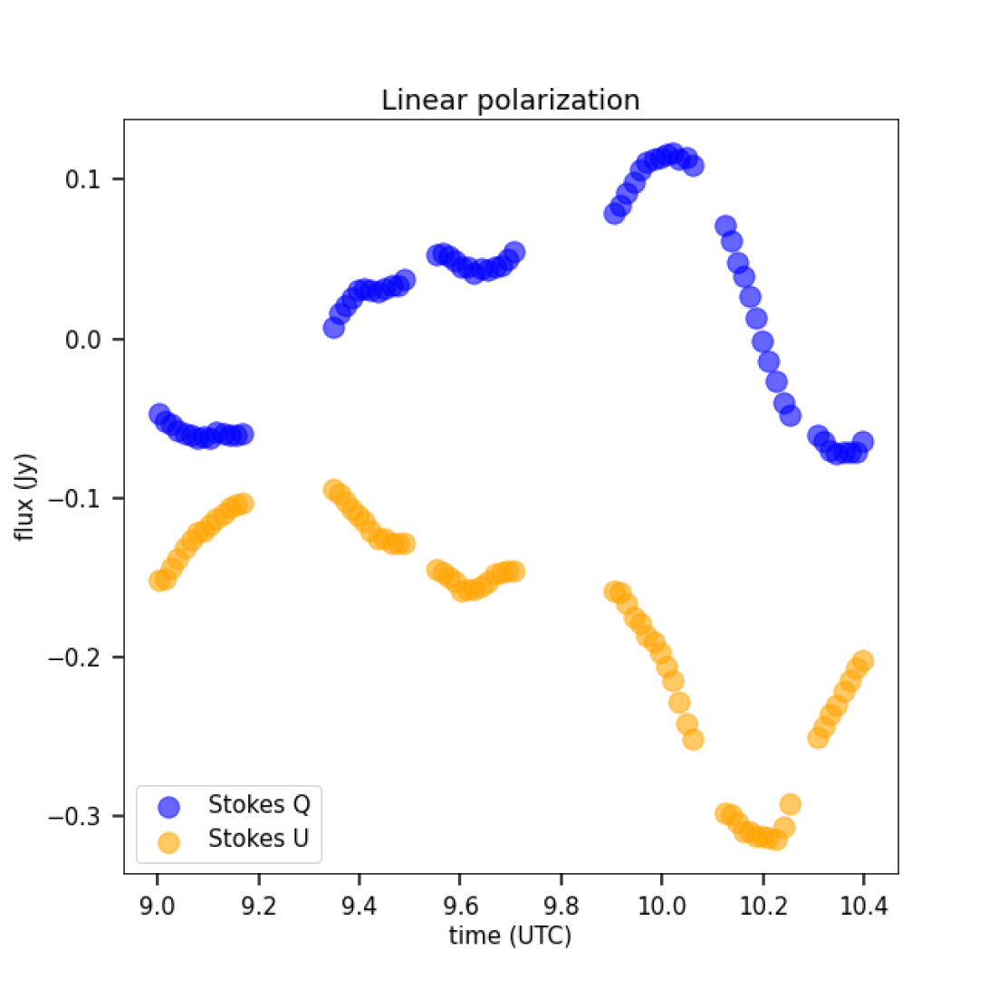
Figure 1: Observed Sgr~A* light curves for Stokes $\mathcal{Q}$ and $\mathcal{U}$ from ALMA (W22). We have plotted only the 71 points, used in this work to infer model parameters, instead of the 710 points from the original light curve.

2 Model

Table 1: Parameters and prior ranges used for the fitting. All priors are flat apart from $n_{0,s}$, $\Theta_{0,s}$, $B_{0,s}$, $C_{\textrm{coef}}$, where we used truncated log-normal priors centered at the middle of the corresponding ranges.

Parameters	Ranges	Description
i	$[90-180^{\circ}]$	Viewing angle (inclination) of the observer: $i=0^{\circ}$ is face-on, $i=90^{\circ}$ is edge-on
$a_{*}$	$[0-1)$	Dimensionless black hole spin
$n_{0,s}$	$[10^{4}-10^{8}]$	Electron number density at the center of the spot (cm-3)
$\Theta_{0,s}$	$[1-10^{3}]$	Electron dimensionless temperature at the center of the spot
$B_{0,s}$	$[0.1-10^{2}]$	Magnetic field strength $(G)$
$r_{s}$	$[7-15]$	Distance of the center of the spot from BH center ($M$)
$\phi_{\rm cam}$	$[0-360^{\circ}]$	Location of the camera at the first point of observation (shifts light curves left-right)
$Q_{\rm sha}$	$[-1,1]$	Average background Stokes $Q$ parameter (Jy)
$U_{\rm sha}$	$[-1,1]$	Average background Stokes $U$ parameter (Jy)
PA	$[0-360^{\circ}]$	Position angle of the black hole spin projected on the observer’s screen, measured east of north
$C_{\textrm{coef}}$	$[10^{-5}-10^{-3}]$	Coefficient for the exponential cooling ($M^{-1}$)
$K_{\textrm{coef}}$	$[0.5-1.2]$	Coefficient defining the orbital velocity with respect to the Keplerian case

To simulate millimeter emission from flaring Sgr~A* we adopt and further develop the semi-analytic model described in full detail by Vos et al. (2022). The model is inspired by work of Broderick & Loeb (2006), see also Fraga-Encinas et al. (2016). It consists of a semi-analytic model of a stationary accretion flow and a time-dependent component of an orbiting bright spot around a Kerr BH. The model is fully built within ipole, a ray-tracing code for covariant general relativistic transport of polarized light in curved spacetimes developed by Mościbrodzka & Gammie (2018). ipole code has been used, among other applications, to generate EHT library of template black hole images based of GRMHD simulations (e.g., EHTC et al. 2022d).

To calculate thermal synchrotron emission (we assume that electrons have a relativistic thermal energy distribution function, see Vincent et al. 2023 for a different approach), the radiative transfer model necessitates the specification of the plasma’s underlying density, electron temperature, and magnetic field characteristics. Once the plasma configuration is defined, ipole generates maps of Stokes ${\mathcal{I},Q,U}$, and $\mathcal{V}$ at the selected observing frequencies. The underlying calculations employ the full relativistic radiative transfer model of ipole, including synchrotron emission, self-absorption, and the effects of Faraday rotation and conversion. Since Sgr A* indicates a moderate Faraday depth at 230 GHz, with a Faraday screen most likely collocated with the compact emission region (Wielgus et al., 2023), it may be necessary to incorporate complete radiative transfer into the model for quantitative comparisons with observations. We self-consistently account for the finite velocity of light, that is, we do not employ the commonly used fast light approximation.

The model is divided into two components: a static background, modeling a radiatively inefficient ADAF disk, and an orbiting hot spot. For the background variables we use the ”bg” subscript and the governing equations read as

$$n_{e,bg} = n_{0,bg}\left(\frac{r}{r_{g}}\right)^{-1.5}\exp{\left(\frac{-\cos^{2}{\theta}}{2\sigma^{2}}\right)}\,,$$

$$\Theta_{e,bg} = \Theta_{0,bg}\left(\frac{r}{r_{g}}\right)^{-0.84}\,,$$

$$B_{bg} = B_{0,bg}\left(\frac{r}{r_{g}}\right)^{-1}\,,$$ (1)

where $n_{e}$ is the electron number density, $\sigma=0.3$ characterizes the disk vertical thickness, $\Theta_{e}=k_{b}T_{e}/m_{e}c^{2}$ is the dimensionless electron temperature, $B_{bg}$ is the magnetic field strength, $r_{g}=GM/c^{2}$ is the gravitational radius, $r$, $\theta$ are the coordinates and $n_{0,bg}$, $\Theta_{0,bg}$, $B_{0,bg}$ are the values at the center (r=0). The field has a vertical orientation, unless specified otherwise (poloidal, or radial possibilities) with one of two possible polarities. The background ADAF is either on a fixed Keplerian orbit or deviating from it according to the parameter $K_{\textrm{coef}}$ that corresponds to a period $P$ of

$$P=\frac{2\pi}{K_{\textrm{coef}}}\frac{r_{g}}{c}\left(\left(\frac{r}{r_{g}}\right)^{1.5}+a_{*}\right),$$ (2)

where $K_{\textrm{coef}}$ is a parameter controlling the Keplerianity of the orbit (for $K_{\textrm{coef}}=1$ the disk orbit is Keplerian, for $K_{\textrm{coef}}<1$ it is sub-Keplerian). In our model, all emission is cut below the inner most stable circular orbit (ISCO). The spacetime is described with the Kerr metric, with the standard metric signature $(-\,+\,+\,+)$ and dimensionless BH spin $a_{*}=Jc/GM^{2}$. The units are natural ($c=G=1$), hence distance and time can be conveniently measured in units of $M$ $(M\equiv r_{g}\equiv r_{g}/c)$. We assume a mass of Sgr A* $M=4.155\times 10^{6}\,M_{\odot}$, which is between the measurements of GRAVITY Collaboration et al. (2022) and Do et al. (2019).

The second component of the model is the spot. The spot lies in a circular orbit in the equatorial plane and its location in Kerr-Schild coordinates is defined as

$$\mathrm{x}_{s}^{0} = t\,,$$

$$\mathrm{x}_{s}^{1} = r_{s}\,,$$

$$\mathrm{x}_{s}^{2} = \pi/2\,,$$

$$\mathrm{x}_{s}^{3} = 2\pi t/P\,.$$ (3)

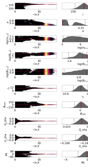
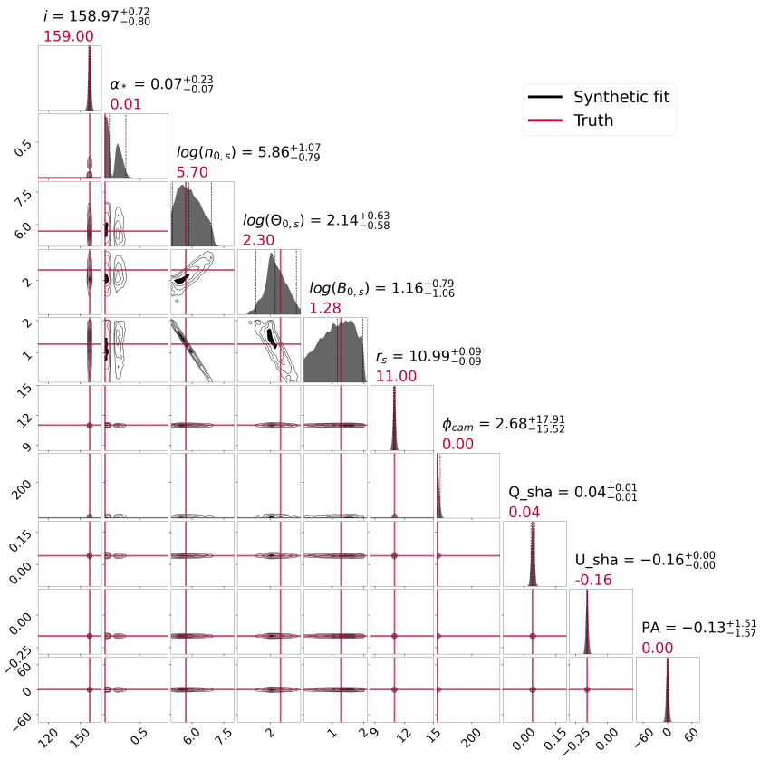
Figure 2: The trace and triangle plots of the synthetic light curve fitting. The trace plot, on the left, shows the evolution of particles (and their marginal posterior distributions) in 1-D projections, where $\ln X$ denotes the prior volume of the parameter space. The dots are color coded with respect to their relative posterior mass, meaning that bright yellow values are present when convergence is achieved. The triangle plot is a combination of 1-D and 2-D marginalized posteriors, with the dashed lines denoting the median and 2- $\sigma$ or (90$\%$) confidence levels (left and right). Similarly the contours are for $90\%$ (outer) and then $50\%$ and $25\%$ confidence levels. The truth is marked with red lines.

Here $t$ is coordinate time (in units of $M$), $r_{s}$ is the radial distance from the BH center (also in units of $M$) and P is the orbital period defined in Eq. 2.

The plasma density, temperature and magnetic field strength in the spot are then described by

$$\begin{aligned} &n_{e,s}=n_{0,s}\exp\left(-\frac{(\Delta x)^{2}}{2R_{s}^{2}}\right),\\ &\Theta_{e,s}=\Theta_{0,s}\exp\left(-\frac{(\Delta x)^{2}}{2R_{s}^{2}}\right)\exp(-C_{\textrm{coef}}(t+T_{\textrm{ini}})),\\ &B_{s}=B_{0,s}\exp\left(-\frac{(\Delta x)^{2}}{2R_{s}^{2}}\right)\,,\end{aligned}$$ (4)

where $n_{0,s}$, $\Theta_{0,s}$, $B_{0,s}$ are the values at the center of the spot, $\Delta x$ is the Euclidean distance from the spot center to the photon’s emission site, connected to the distant observer’s screen with a null geodesic. $R_{s}$ is the size of the Gaussian standard deviation, defining the size of the spot, and it remains fixed at $3M$ to limit the number of parameters. Additionally we use a spot boundary, ignoring matter if $n_{e,s}\leq 0.01n_{0,s}$ to limit the Gaussian tail.

In this work we extend the spot models of Vos et al. (2022) and allow the Gaussian spot to change its temperature as an exponential function of time. This is a general prescription that enables us to explore the impact of cooling without making additional assumptions regarding its physical mechanisms. We introduce the cooling coefficient $C_{\textrm{coef}}$ and the numerical parameter $T_{\rm{ini}}=2000M$ which guarantees that the spot is cooling when $C_{\textrm{coef}}>0$ (notice that ipole tracks light backwards in time from camera position at $r=1000M$ so the coordinate time $t$ is a negative quantity). The spot is not cooling when $C_{\textrm{coef}}=0$.

There are two remaining numerical parameters of our model: the image field-of-view (FOV) and its resolution. We adopt FOV=40$M$$\approx 200\,\mu$as, because most of the millimeter emission of Sgr~A*   is generated close to the black hole event horizon, with the BH shadow ring diameter observed by the EHT corresponding to around 10-11$M$ (EHTC et al., 2022a, e). Synthetic light curves are then generated by creating snapshot images at a predefined sequence of times and integrating their intensities over the FOV into total flux densities in all four Stokes parameters. Due to large numerical cost of these calculations, we adopted resolution of 16$\times$16 pixels per single frame. An analysis of the effects of image resolution on simulated light curves can be found in Appendix A, where we justify the low value of the chosen resolution. Our reasoning being that despite some fractional differences in some parts of the curves, the general behavior remains very similar.

3 Two-step parameter estimation procedure

ALMA observed Sgr~A* on April 11, 2017 from 9 UTC until 13 UTC. Stokes $\mathcal{Q}-\mathcal{U}$ loops, interpreted as a signature of a bright spot around the black hole, were observed within the first two hours of this observing window. We fit ALMA light curves starting at 9:00 UTC until 10:30 UTC (see Fig. 1). Hence, the data segment we consider begins 20 min earlier than the segment used by W22. Our original data set has 710 data points. Notice that within this time ALMA data has a few gaps in which it was observing Sgr~A* calibrators. In our modeling, we only fit Stokes $\mathcal{Q}$ and $\mathcal{U}$ light curves but we verify Stokes $\mathcal{I}$ and ${\mathcal{V}}$ for consistency afterwards. This is because we assume that during the $\mathcal{Q}-\mathcal{U}$ loop the strongest signal of the spot is visible in the linear polarization rather than in total intensity and circular polarization, which may be dominated by the black hole shadow component originating close to the event horizon of the black hole and associated with the background image of the accretion flow (W22).

To model the presented ALMA data, we set up a fitting framework that combines our ipole simulations with dynesty software, introduced by Speagle (2020) and further developed by Koposov et al. (2023). dynesty is a Bayesian tool capable of performing dynamic nested sampling, introduced for computational usage in Skilling (2006). Given our model light curves, dynesty proves to be an excellent choice for our framework due to its compatibility with low-dimensional yet highly degenerate and potentially multimodal posteriors (e.g. Palumbo et al. 2022). We embedded ipole in a way that the sampler calls a ray-tracing operation for every log-likelihood evaluation.

The posterior landscape of our model is very complex and our model for the background emission (the shadow component) neither includes emission from regions within the ISCO nor has any variability, therefore we decided to simplify our fitting procedure. We introduce a two-step fitting scheme in which the spot light curve is fitted separately from static background emission as follows. In our first fitting step, we fit emission from the spot alone and in this step the background linear polarization is modeled as $\mathcal{Q}_{sha}$ and $\mathcal{U}_{sha}$ parameters (where $sha$ stands for shadow, following W22) which are simply added to the variable light curves. In our second fitting step, we fit the static background model to the estimated pair of (${\mathcal{Q}}_{sha}$,${\mathcal{U}}_{sha}$) which represents an average emission from near the shadow of the black hole that is always visible in the millimeter waves. Such split in the fitting procedure works well as long as both Faraday effects between components are negligible, for example, if both model components are spatially separated in the images. As shown later in this paper, our spot is usually located at $r>10$$M$ with very narrow posterior distributions so the spot and the near horizon emission are usually well separated.

To be able to produce a fit on timescales $\ll$ than a PhD student lifetime, we sub-sample the ALMA data set of W22 by a factor of 10, changing minimal cadence from 4 s to 40 s. Hence, we fit only 71 data points (or rather 142, since we take into account $\mathcal{Q}$ and $\mathcal{U}$ values separately). Because of the temporal correlation timescales involved the subsampling has little impact on the inference power. Eventually we ended with a scheme that performs a single log-likelihood evaluation in less than 2 seconds, using 24 cores.

The time per log-likelihood calculation requires a configuration for dynesty that converges with the least amount of iterations. For that we use a dynamic sampler, introduced by Higson et al. (2019) with 200 initial live points and 200 points per extra dynamical batch (10 in total). We use the default stopping criteria, meaning a terminating change in the log-evidence of 0.01. Additionally we adopt a weight function that shifts the importance of the posterior exploration (rather than the evidence) to $100\%$. Lastly we use overlapping balls that can generate more flexible bounding distributions, first mentioned in Buchner (2016), and random walk as our sampling technique developed by Skilling (2006).

Our log-likelihood function is defined in a standard way as:

$$\mathcal{L}(\@vec{p})=-\sum_{j}\frac{\left[Q_{j}-\hat{Q}_{j}(\@vec{p})\right]^{2}}{2\sigma_{Q,j}^{2}}+\frac{\left[U_{j}-\hat{U}_{j}(\@vec{p})\right]^{2}}{2\sigma_{U,j}^{2}}\,$$ (5)

where $\@vec{p}$ is the vector of parameters to estimate, $Q_{j}\,,U_{j}$ and $\hat{Q}_{j}(\@vec{p})\,,\hat{U}_{j}(\@vec{p})$ are the observed and modeled Stokes ${\mathcal{Q}}$ and ${\mathcal{U}}$ for every data point ($j$). The modeled quantities are directly calculated during the ray-tracing. The errors have been defined as

$$\sigma_{Q,j} = \epsilon_{s}|Q_{j}|+\epsilon_{t}\,,$$

$$\sigma_{U,j} = \epsilon_{s}|U_{j}|+\epsilon_{t}\,,$$ (6)

where $\epsilon_{s}=0.02$ is the assumed systematic error and $\epsilon_{t}=0.01$ represents thermal noise, see Wielgus et al. 2022a for the characterization of uncertainties in the ALMA data set. The reduced $\chi^{2}$ then naturally follows as:

$$\chi_{\rm eff}^{2}=\frac{\chi^{2}}{n_{d}-n_{f}}$$ (7)

where $\chi^{2}=-2\mathcal{L}$, $n_{d}=142\,,(2\times 71)$ is the number of data points and $n_{f}=10,\,11$ or $12$, the number of degrees of freedom, equal to the number of parameters being fitted simultaneously.

A comprehensive list of all the parameters and their ranges used in our fitting pipeline, referred to as bipole in the next sections, is shown in Table LABEL:tab:params. For $n_{0,s},\,\Theta_{0,s}$ and $B_{0,s}$ we sample the log space with Gaussian priors centered at the middle of their log ranges (i.e. log-normal priors). For the rest of considered parameters we assume flat priors.

Finally, before fitting the real data we perform a controlled bipole run using synthetic data to demonstrate the ability of our pipeline to recover the Truth value. In this run we use the parameters proposed by W22 to recreate their model. The total number of fitted parameters is the same as for the real data (see Section 4) with the same priors. The results of this run are presented in Fig. 2. On the left side we present the trace plot, showing the evolution of the live points throughout the run. On the right side the corner (or triangle) plot, showing the single and joint distributions for all parameters. All Truth values, indicated with red lines, are comfortably covered by the posteriors. Additionally, we observe a correlation between density, temperature, and magnetic field strength ($n_{0,s}\,\Theta_{0,s},\,B_{0,s}$) which is expected for synchrotron emission, with emissivity coefficient depending on all three physical quantities.

4 Results

4.1 Spot fitting

Table 2: Models used for fitting Sgr A* ALMA data.

Model ID	$B_{\rm field}$	Cooling	Keplerian	Parameters
nc_b	default	no	yes	10
nc_fb	flipped	no	yes	10
c_b	default	yes	yes	11
c_fb	flipped	yes	yes	11
nc_b_nk	default	no	no	11
nc_fb_nk	flipped	no	no	11
c_b_nk	default	yes	no	12
c_fb_nk	flipped	yes	no	12

We run eight models, listed in Table LABEL:tab:models, to fit the spot component to the ALMA observational data. The set of models is composed of all combinations of the three criteria: 1) no cooling or fitting the cooling parameter $C_{\rm coef}$; 2) prescribed default or flipped magnetic field orientation (polarity; note that in the default models the magnetic field vector is aligned with the black hole spin, which is also aligned with the hot spot’s angular momentum vector); 3) assumed Keplerian motion, or fitting a non-keplerianity parameter $K_{\rm coef}$. The models are labeled to contain the information of the specific case; first part refers to cooling (nc being no cooling), second to $B_{\textrm{field}}$ (fb being flipped field) and the last to Keplerian orbit (nk being non-Keplerian orbit). In what follows we report the posteriors from each run, we discuss the goodness of the fit and we show the produced light curves with the best parameters from every model.

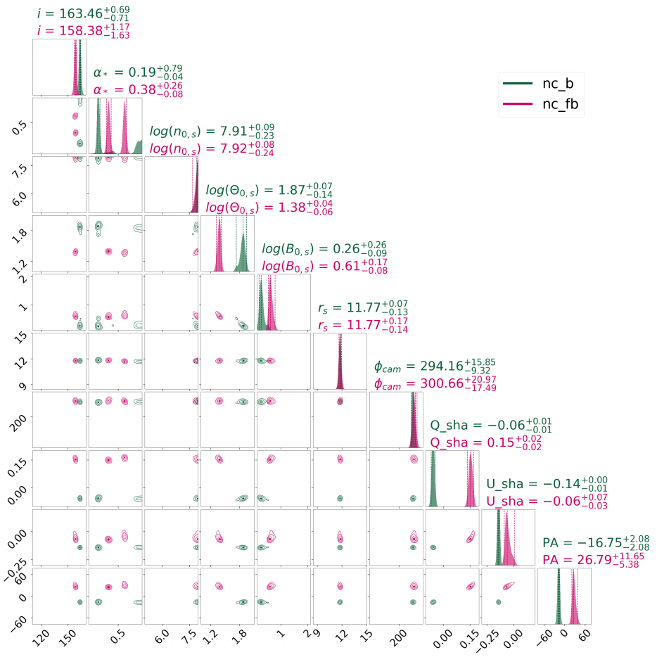
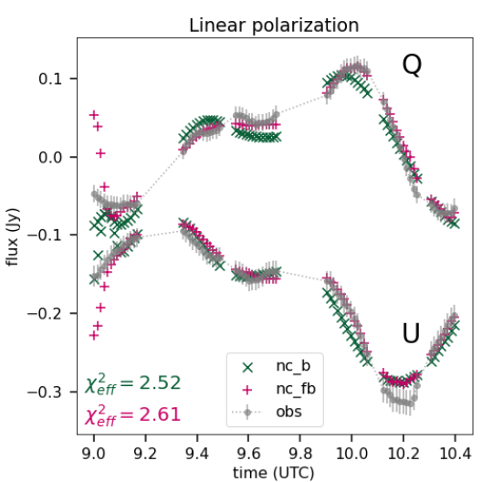
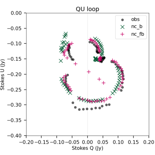
Figure 3: Top: Triangle plot of posterior distributions for all parameters considered in Keplerian spot models without cooling ($K_{\rm coef}=1$, $C_{\rm coef}=0$). Results for both magnetic field polarities are shown in different colors. Bottom: best-fit model $\mathcal{Q}-\mathcal{U}$ light curves and $\mathcal{Q}-\mathcal{U}$ loops (color points) overplotted with ALMA observational data (gray points).

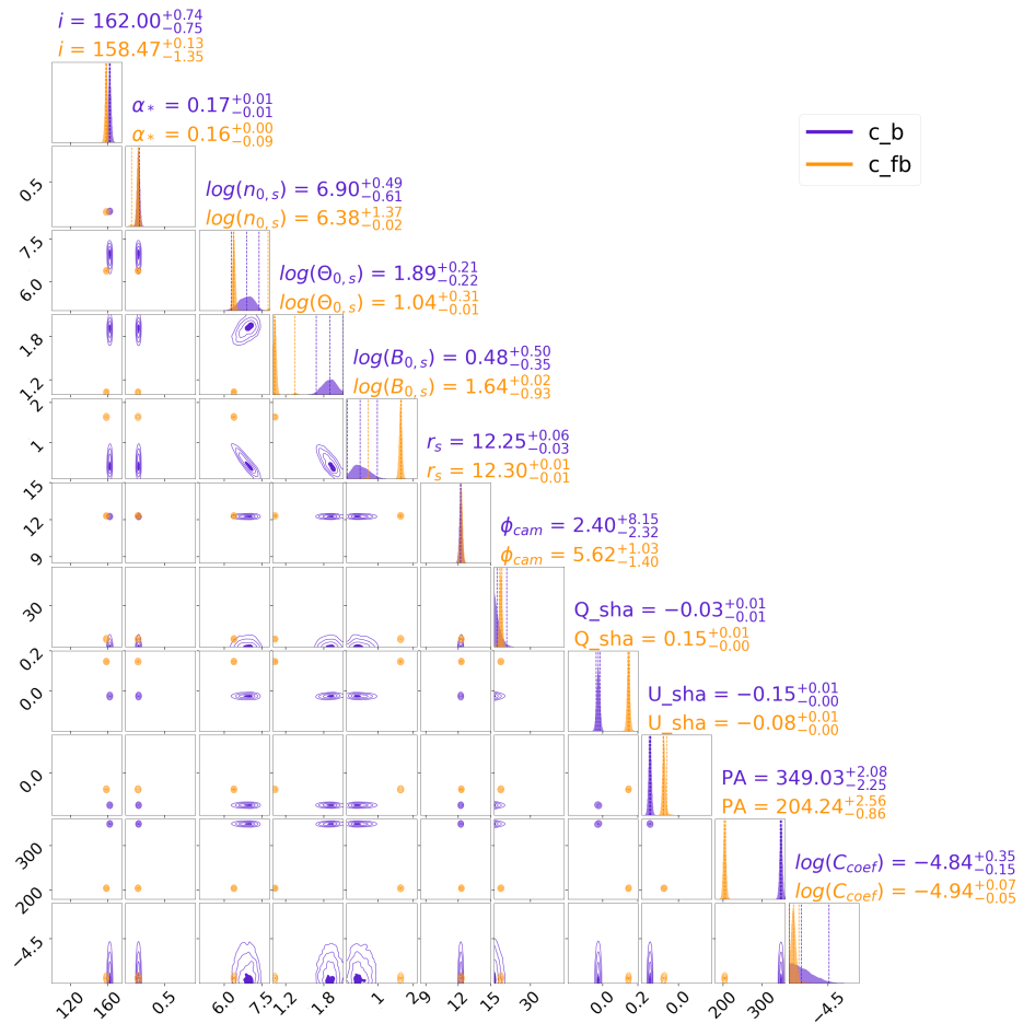
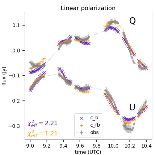
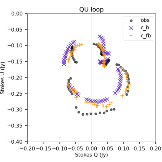
Figure 4: Same as in Fig. 3 but for Keplerian models with cooling included ($K_{\rm coef}=1$, $C_{\rm coef}\neq 0$).

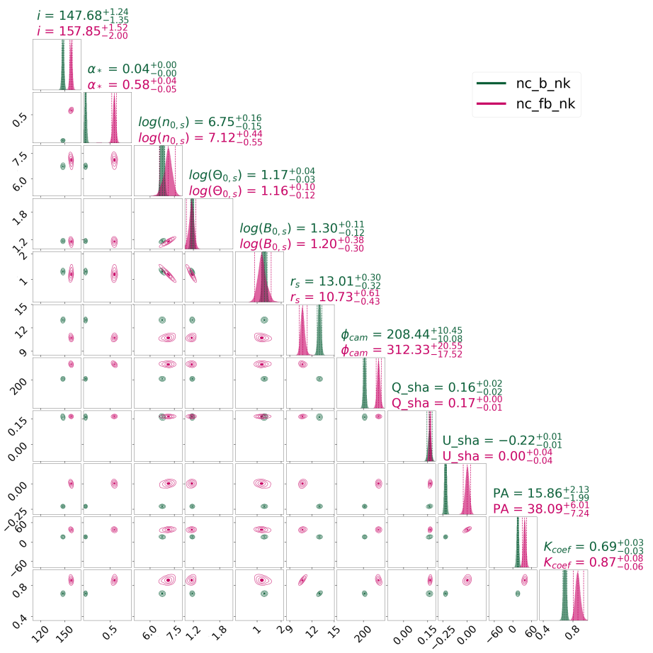
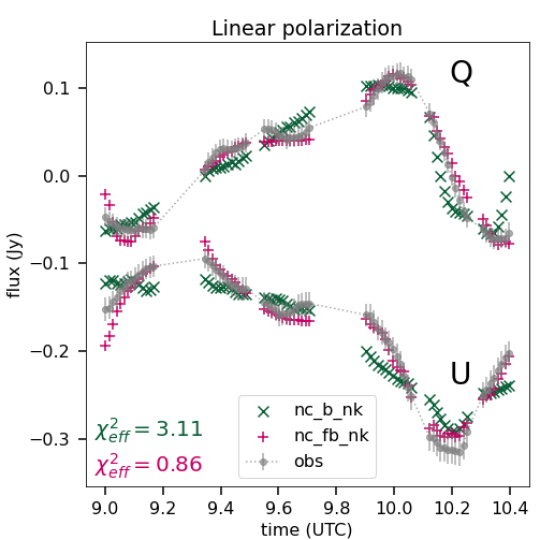
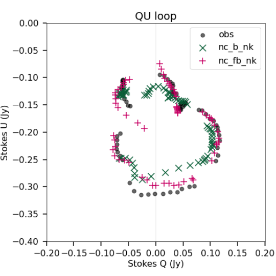
Figure 5: Same as in Fig. 3 but for non-Keplerian models without cooling included ($K_{\rm coef}\neq 1$,$C_{\rm coef}=0$).

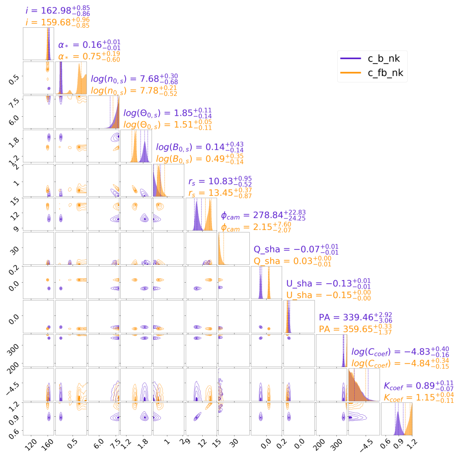
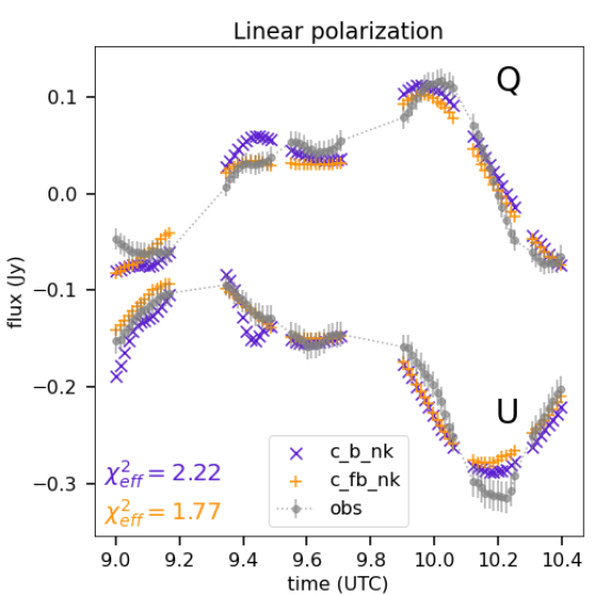
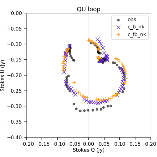
Figure 6: Same as in Fig. 3 but for non-Keplerian models with cooling included ($K_{\rm coef}\neq 1$, $C_{\rm coef}\neq 0$).

In Fig. 3 (top part) we show the posterior distributions for all parameters for two different magnetic field orientations in Keplerian models without cooling (nc_b, nc_fb). The first important feature to note is the agreement in the value of inclination for both models, matching the fiducial model of W22, which assumed 158 deg inclination. Secondary, the values of $r_{s}$ are identical between models ($r_{s}=11.77$$M$ and with narrow posteriors), but larger than W22, who assumed 10-11M. This has a direct effect on the loop period (Eq. 2, for $r_{s}\sim 10$$M$ and fixed Keplerian motion spin has little effect), producing a period of $T=87-93$min, longer than the 70min proposed in W22. This will be further discussed in the next Section 5. The spin showcases multimodal distributions with most weight on the lower end, but still not well constrained. The fluid parameters are presented in normal distribution with $n_{0,s}$ being on the very high end of the priors, and $\Theta_{0,s}$, $B_{0,s}$ exhibiting a noticeable shift between the two cases, as well as the $Q_{\rm sha},U_{\rm sha}$ values (see Sec. 4.3). There is a correlation between $n_{0,s}$, $\Theta_{0,s}$ and $B_{0,s}$ but not as strong as in the synthetic data fit. The PA values lay around zero. In the bottom part of Fig. 3 we present the light curves and the $\mathcal{Q}-\mathcal{U}$ loop using the peak of the posteriors from each run as parameters for the ray tracing. In the lower left corner of the light curve we report the lowest $\chi_{\rm eff}^{2}$ value. The two models have nearly the same value of $\chi^{2}_{\rm eff}$, despite the first few points being mismatched in the nc_fb case. If we disregard the first 3 points, the value of $\chi_{\rm eff}^{2}$ drops to $\chi_{\rm eff}^{2}=0.67$, proving an even better fit.

For the second family of models used in the fitting pipeline (c_b, c_fb) we incorporate an extra parameter, namely $C_{\textrm{coef}}\neq 0$, that permits for time evolution of the electron temperature values in the spot according to Eq. 4. In Fig. 4 (top panels) we show the posterior distributions for all free parameters of this model. Again, the inclination is consistent between the two orientations of $B_{\rm field}$, and with the no-cooling models nc_b and nc_fb. The spin and electron density ($n_{0,s}$) are in similar values between $B_{\rm field}$ orientations and they are lower than the no-cooling counter parts (an order of magnitude for $n_{0,s}$). Additionally, the spin does not exhibit any bimodality and is well constrained in the low end of the prior range. The radius is even larger, but still in agreement between $B_{\rm field}$ orientations ($r_{s}=12.25-12.30$ $M$). Then the two remaining astrophysical parameters ($\Theta_{0,s}$ $B_{0,s}$) have significant shifts between the two $B_{\rm field}$ orientations, with the highest magnetic field strength observed for the flipped field ($B_{0,s}=43\,G$). The shadow parameters are comparable with the no-cooling models. The cooling coefficient for both runs is $C_{\textrm{coef}}\sim 10^{-5}$ producing a drop in temperature of roughly $1\%$ during the simulation (notice that the model light curve length is $\sim$1.4h). In bottom panels of Fig. 4 we present model c_b and c_fb light curves and the $\mathcal{Q}-\mathcal{U}$ loop using the peak of the posteriors from each run as parameters for the ray tracing with the lowest $\chi_{\rm eff}^{2}$ reported in the lower right corner of the figure. Once again, the flipped $B_{\textrm{field}}$ seems to reproduce the data better, reflected in the $\chi_{\rm eff}^{2}=1.21$, nearly half the value of default $B_{\textrm{field}}$ and nearly half the value for Keplerian spot models without cooling.

In Fig. 5 (top panels) we show the posterior distributions for all free parameters for non-Keplerian model without cooling (models nc_b_nk and nc_fb_nk with $K_{\textrm{coef}}\neq 1$, $C_{\textrm{coef}}=0$). The differences between the two $B_{\textrm{field}}$ orientations are significantly enhanced. The most evident discrepancies are in $i$, $r_{s}$ and $K_{\textrm{coef}}$. These create diverse light curves, as can be seen in the bottom panels of Fig. 5. In particular the relation of $r_{s}$ with $K_{\textrm{coef}}$ for nc_b_nk is counter-intuitive, since we would expect sub-Keplerian orbits to occur at smaller orbits, to keep the period of the spot fixed. Clearly, the default $B_{\textrm{field}}$ models have a harder time reproducing the data with the addition of the Keplerian freedom.

In Fig. 6 (top panels) we show the posterior distributions for all free parameters for non-Keplerian model with cooling (models c_b_nk and c_fb_nk with $K_{\textrm{coef}}\neq 1$, $C_{\textrm{coef}}\neq 0$,). The particularity in this case is that model c_fb_nk is the only one to exhibit a super-Keplerian orbit, followed by a larger orbit to maintain the period. The light curves created with the peaks of the parameters posteriors are shown in Fig. 6 bottom panels. Both shown light curves show agreement with the data with typical $\chi_{\rm eff}^{2}$ values, around 2.

The orbital periods of most of the best-fit models (with just one exception) fall into a narrow range between 87 and 93 minutes which corresponds to the duration of our fitted lightcurve (1.5h). One non-Keplerian model (with default $B_{\rm field}$ orientation and no cooling) has much longer period of approximately 145 minutes. All spot orbital periods are reported in Table LABEL:tab:logz in Section 5.

4.2 Cross-checking with other Stokes parameters

In this section we report the behavior of the Stokes $\mathcal{I}$ and $\mathcal{V}$ light curves for the best-fit realisations of the eight discussed models. The goal is to verify consistency of the models with the remaining observational information that is not used in the fitting procedure due to the model limitations listed in Sect. 3.

In Fig. 7, top row, we present the Stokes $\mathcal{I}$ light curves for all spot models. The shift (sha) of the light curves is just for visual aid, and accommodates the contribution we expect from the background, meaning the disk. We have not fitted for the best shadow (sha) values to Stokes $\mathcal{I}$ (and $\mathcal{V}$, see below). We observe only a small variation in Stokes $\mathcal{I}$ in all models. That is expected since Stokes $\mathcal{I}$ should be largely dominated by the background emission and any variations could be due to the background variability which we do not model here.

In Fig. 7, bottom row, the light curves for Stokes $\mathcal{V}$ are shown. All models with flipped $B_{\textrm{field}}$, apart from one, exhibit a rich behavior with variations in the light-curve that closely resemble the observational data. By applying a shift with the same ”shadow” concept as for Stokes $\mathcal{I}$ the coincidence with the data is evident. The ability of some of our models to recover the observed Stokes $\mathcal{V}$ is a strong independent argument in support of the model.

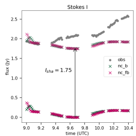
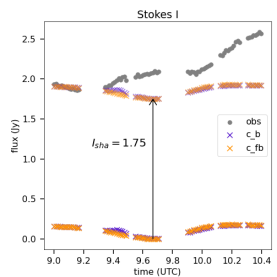
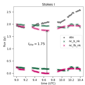
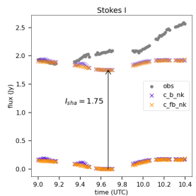
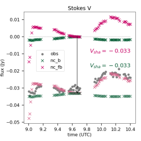
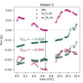
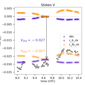
Figure 7: Stokes $\mathcal{I},\,\mathcal{V}$ light curves for all models compared to the observational data from Wielgus et al. (2022a) and W22 (obs). The arrows represent a constant background component to facilitate comparison with the real data.

4.3 Background emission

Here we report the second part of our two-step fitting algorithm. We fit the $\mathcal{Q}_{\textrm{sha}}$, $\mathcal{U}_{\textrm{sha}}$ values from every model (reported in Table LABEL:tab:QU_sha) with the ADAF model described by Eqs. 1. Our goal is to obtain the density, temperature and magnetic fields’ strength of the background component. The plasma parameters of the background emission fitting is carried out in two ways: i) we fix all the geometric parameters ($a_{*}$, $i$, PA), plus $K_{\rm coef}$ for non-Keplerian models, at the values obtained in the spot fitting (during the first step); ii) we fit the geometrical parameters ($a_{*}$, $i$, PA), plus $K_{\rm coef}$ for nk models, to the $\mathcal{Q}_{\textrm{sha}}$, $\mathcal{U}_{\textrm{sha}}$ together with other background parameters in order to check if they converge to the values obtained in the first (spot) fitting step. Notice that since the background is static we only need one point (or rather two, for Q and U) to make the fit.

Table 3: The $\mathcal{Q}_{\textrm{sha}}$, $\mathcal{U}_{\textrm{sha}}$ values for all models obtained in the first fitting step, as well as the average values of $\mathcal{Q}$ and $\mathcal{U}$ from the ALMA data.

Model ID	$Q_{\textrm{sha}}$ (Jy)	$U_{\textrm{sha}}$ (Jy)
nc_b	$-0.08$	$-0.13$
nc_fb	$0.15$	$-0.06$
c_b	$-0.3$	$-0.15$
c_fb	$0.15$	$-0.08$
nc_b_nk	$0.16$	$-0.22$
nc_fb_nk	$0.17$	$0.00$
c_b_nk	$-0.07$	$-0.13$
c_fb_nk	$0.03$	$-0.15$
ALMA average	$0.015$	$-0.18$

In Figures 8 and 9 we show the posteriors from all aforementioned background models. All runs converge, but it is clear that there is a high level of correlation mostly for the 6 and 7 parameter ones and lower for the 3 parameters. Furthermore, in the nc_b 3 parameters case the correlation is higher than nc_b_nk, probably due to the low value of $K_{\rm coef}=0.69$ making it harder for the background to meet the Stokes $\mathcal{Q}_{\textrm{sha}}$, $\mathcal{U}_{\textrm{sha}}$ values. The values for $n_{0,bg}$, $\Theta_{0,bg}$ and $B_{0,bg}$ are in similar levels as the spot models, but according to Eq. 1 that would make them roughly 10 times smaller at the location of the spot ($r\sim 10M$). For the 6 and 7 parameter models the peaks of geometric parameters deviate from the spot models fits, but the posteriors are able to cover the same values, apart from PA.

Using the peaks of the posteriors from the 3 parameter runs, we have calculated Stokes $\mathcal{I}_{\textrm{BG}}$, $\mathcal{V}_{\textrm{BG}}$ produced from the background disk. Our motivation is to test if any of the Stokes values match the reported $\mathcal{I}_{\textrm{sha}}$, $\mathcal{V}_{\textrm{sha}}$ values, used in Fig. 7. The values are reported in Table LABEL:tab:IV. It is clear that both $\mathcal{I}_{\textrm{BG}}$, $\mathcal{V}_{\textrm{BG}}$ are overestimated. On top of that, the models with flipped magnetic field orientation produce opposite values for Stokes $\mathcal{V}_{\textrm{BG}}$. We comment on the implications of these results in Section 5. Overall, this second step does not offer much inferring power at this point, but it serves well as a sanity check and validation of our overall approach of splitting the fitting into two steps.

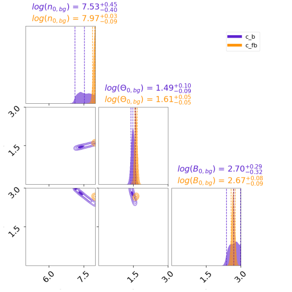
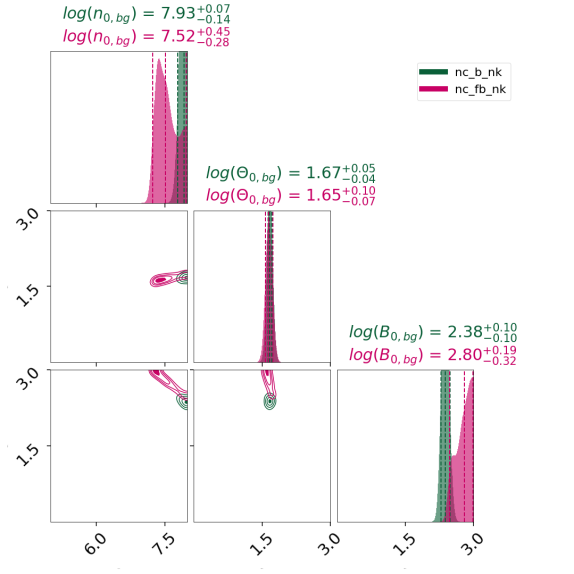
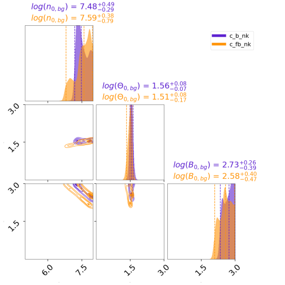
Figure 8: Triangle plots for background solution, keeping geometric parameters ($i,a$, PA), and $K_{\rm coef}$ for nk cases, fixed at the values of the initial runs for both $B_{\textrm{field}}$ orientations (color coded) and without (left panels) and with cooling (right panels).

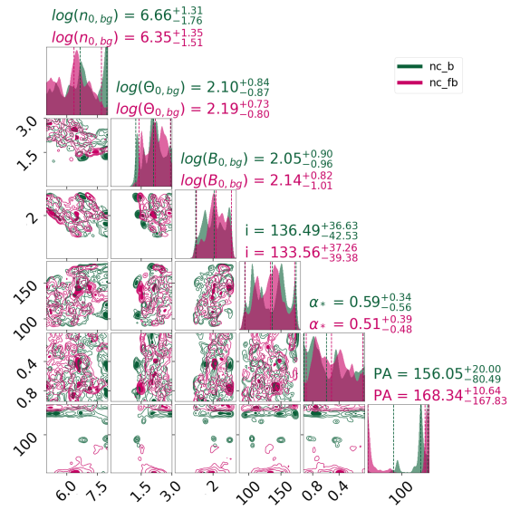
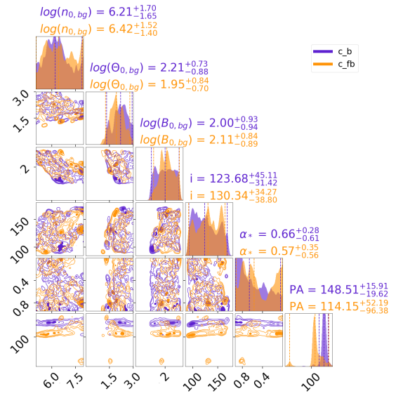
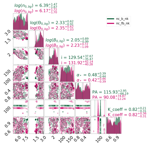
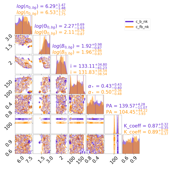
Figure 9: Triangle plots for background solution, letting geometric parameters ($i,a$, PA) run separately from the initial spot runs for both $B_{\textrm{field}}$ orientations (color coded) and without (right panels) and with cooling (left panels).

Table 4: The $\mathcal{I}_{\textrm{BG}}$, $\mathcal{V}_{\textrm{BG}}$ values for all models obtained in the second fitting step (3 parameters), directly compared to the $\mathcal{I}_{\textrm{sha}}$, $\mathcal{V}_{\textrm{sha}}$ used for visual aid in Fig. 7, as well as the average values of $\mathcal{I}$ and $\mathcal{V}$ from the ALMA data. Note that the average of $\mathcal{I}$ is from the first 10 points since the later increase in Stokes $I_{\textrm{sha}}$ is argued to occur due to the time evolution of the background or the spot-background interactions.

Model ID	$I_{\textrm{BG}}$ (Jy)	$V_{\textrm{BG}}$ (Jy)	$I_{\textrm{sha}}$ (Jy)	$V_{\textrm{sha}}$ (Jy)
nc_b	$1.01$	$-0.019$	$1.75$	$-0.033$
nc_fb	$2.55$	$+0.28$	$1.75$	$-0.033$
c_b	$2.32$	$-0.25$	$1.75$	$-0.025$
c_fb	$6.63$	$+0.64$	$1.75$	$-0.037$
nc_b_nk	$3.46$	$-0.47$	$1.75$	$-0.018$
nc_fb_nk	$8.04$	$+0.91$	$1.75$	$-0.040$
c_b_nk	$3.15$	$-0.34$	$1.75$	$-0.027$
c_fb_nk	$3.36$	$+0.41$	$1.75$	$-0.027$
ALMA average	-	-	$1.90$	$-0.027$

5 Discussion and conclusions

In this work, we generate a family of semi-analytic models of an accretion flow with a bright orbiting spot to fit Sgr A* millimeter data recorded by ALMA on April 11, 2017. Our models have varying number of degrees of freedom. Which model represents the observational data best? One can answer this question using either Bayesian or physical arguments.

The model that reproduces the data best, that is, corresponds to the lowest $\chi^{2}_{\rm eff}$ parameter, can be seen in Fig. 10, made with flipped $B_{\textrm{field}}$, no cooling, and non-Keplerian orbit. Based on $\chi^{2}_{\rm eff}$, three out of four models with the flipped $B_{\textrm{field}}$ (magnetic field vector arrow pointing towards the observer for viewing angles $i>90$ deg) describe the observations better. Additionally, in Table LABEL:tab:logz, we report all the log-Evidence (marginal likelihood) from all models. All flipped $B_{\textrm{field}}$ models have larger Evidence. It is worth noting that model nc_fb has almost as good log-Evidence as our best-fitting model, despite the larger $\chi_{\textrm{eff}}^{2}$, meaning that the fit is good but the $\chi_{\textrm{eff}}^{2}$ is hindered from the first 3 points deviating from the data.

Using physical arguments, models that describe observations best are those which in addition to Stokes $\mathcal{Q}$ and $\mathcal{U}$ also show some consistency with the observed Stokes $\mathcal{V}$ (also see the Appendix E of W22, ). A model which satisfies this requirement particularly well is the one with the spot on a Keplerian orbit, with cooling allowed and with the flipped magnetic field. All models with default magnetic field orientation fail to recover the Stokes $\mathcal{V}$ variability. We also find a mismatch between modeled and observed Stokes $\mathcal{I}$ during the flare, but this is expected. Stokes $\mathcal{I}$ during the flare could be dominated by the background emission, which may be changing as well. Indeed, the observed total intensity light curve appears to recover from the minimum following the X-ray flare, steadily increasing flux density on a timescale of $\sim$2 h, which may be interpreted as the accretion disk cooling down after the energy injection (Wielgus et al., 2022a). Alternatively, Stokes $\mathcal{I}$ during the flare may be also influenced by the spot properties that we do not include in our simple model such as, e.g., shearing of the spot or other spot interaction with the background flow (e.g., Tiede et al., 2020).

In observational data the $\mathcal{Q}-\mathcal{U}$ loop disappears on timescales of about $\sim 2$ h similar as the aforementioned total intensity recovery timescale. Thus, one could argue that the best spot model synchrotron cooling timescale, $T_{\textrm{cool}}$, should also be close to 2 h. Given our best-fit values for $\Theta_{0,s}$ and $B_{0,s}$ we calculate $T_{\textrm{cool}}$ using (W22 and Mościbrodzka et al. 2011):

$$T_{\textrm{cool}}=11\,{\rm h}\left(\frac{B}{10G}\right)^{-2}\left(\frac{\Theta}{50}\right)^{-1}\,.$$ (8)

In Table LABEL:tab:logz, we report $T_{\textrm{cool}}$ values for all spot models. If the disappearance of the spot is due to radiative cooling, then models that match this observational constraint best are the Keplerian model with cooling and reversed magnetic fields ($T_{\textrm{cool}}=$2 h) and the non-Keplerian model without cooling and also with the reversed magnetic fields ($T_{\textrm{cool}}=$2.5 h). Notice, however, that we assume that the electrons in the spot have thermal distribution function. Different assumption, e.g., non-thermal electron distribution function, could lead to different $T_{\textrm{cool}}$.

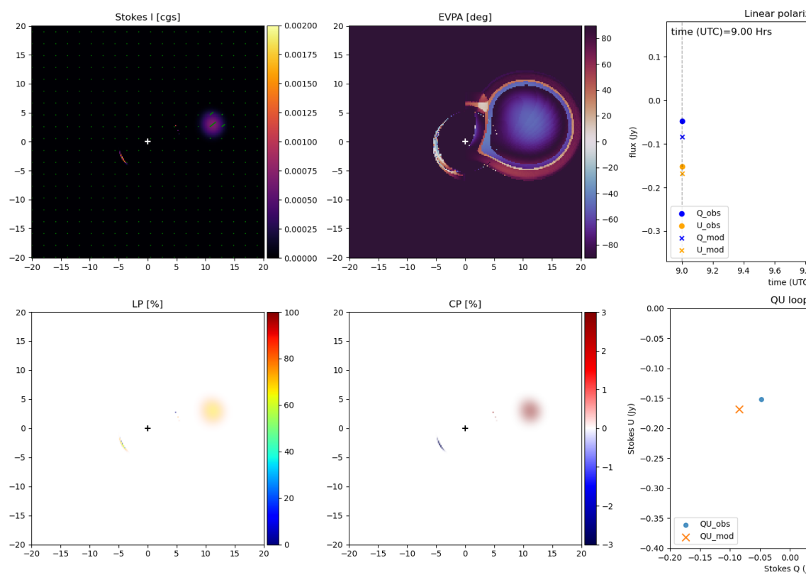
Figure 10: Snapshot from the first point of the light-curve (9:00 UT) from our best fitting model (nc_fb_nk), using $196^{2}$ resolution, for Stokes I, EVPA, fractional linear polarization (LP) and fractional circular polarization (CP).

Regardless of their details, all spot models show consistently similar best fitting viewing angles $i\in(147,163)$ deg and spot orbital radius $r_{s}\in(10,13)M$. The viewing angle close to 180 deg determines a clockwise hot spot rotation on the sky. Such value is also fully consistent with findings of W22 and other independent works (GRAVITY Collaboration et al., 2018, 2020a, 2020b; EHTC et al., 2022d; Gravity Collaboration et al., 2023). For all models (with one exception) the preferred period is approximately 90 minutes (or 145 minutes for the exception) which is longer than 70 minutes estimated by W22. Since we are fitting to a data segment starting at earlier time than W22, a possible interpretation for this discrepancy would be a decrease of the period with time that could result, e.g., from non-negligible radial velocity component of the hot spot inspiring towards the black hole.

For the expected orbital radii, the period (Eq. 2) only weakly depends on black hole spin. Despite of that we obtain a black hole spin estimation of rather moderate values ($a_{*}<0.6$) in all cases. However, in some cases the spin posterior distribution functions are multimodal and therefore they are less certain. In addition to that we do not consider negative spins in our priors, increasing ambiguity on spin estimation. There is also no convincing independent measurement of the Sgr A* black hole spin to compare to. All models, apart from c_fb, also consistently show PA $\in(-20,40)$ deg, meaning that the magnetic field orientation (and, if non-zero, also the black hole spin) may have a specific orientation on the sky. Note that PA corresponds to the position angle of the spin vector projected on the observer’s screen, measured east-of-north (positive PA rotates the image counter-clockwise). In W22 a PA of 57 deg was reported, following a 32 deg counter-clockwise rotation of EVPA, attributed to the external Faraday screen. The existence of the external Faraday screen has been challenged recently by Wielgus et al. (2023), and it is possible that the hot spot orbiting at $r_{s}\approx 11M$ is located outside of the internal Faraday screen zone. In such case no rotation should be applied and the estimate of W22 becomes PA = 25 deg. This value is consistent with the range that we obtained without accounting for the external Faraday screen.

Table 5: Evidence ($\log Z$), $\chi_{\textrm{eff}}^{2}$, period, and cooling timescale $T_{\rm cool}$ (computed using Eq. 8) for all models.

Model ID	Evidence	$\chi_{\textrm{eff}}^{2}$	Period (min)	$T_{\textrm{cool}}$ (h)
nc_b	$-162$	$2.52$	$87.8$	$568$
nc_fb	$-90$	$2.61$	$87.8$	$149$
c_b	$-178$	$2.21$	$93.1$	$79$
c_fb	$-101$	$1.21$	$93.7$	$2$
nc_b_nk	$-172$	$3.11$	$145.3$	$79$
nc_fb_nk	$-89$	$0.86$	$87.6$	$2.5$
c_b_nk	$-183$	$2.22$	$87.2$	$224$
c_fb_nk	$-146$	$1.77$	$93.8$	$90$

All models show consistently that our spot parameters should be in approximate range of $n_{\rm 0,s}\in(2\times 10^{6},8\times 10^{7})$ ${\rm particles/cm^{3}}$, $\Theta_{\rm 0,s}\in(10,77)$, $B_{\rm 0,s}\in(2,40)$ G. Additionally, the non-Keplerian models prefer $K_{\rm coef}\in(0.69,0.9)$, with one exception of $K_{\rm coef}=1.13$. Subsequently, one wonders if the properties of these hot spots can be found in more first-principle numerical (e.g., GRMHD or GRPIC) simulations of ADAFs. GRMHD simulations of Magnetically Arrested Disks (MADs; Narayan et al., 2003) are known to show large-scale disk inhomogeneities threaded by vertical magnetic fields. Such structures, called flux tubes, are associated with magnetosphere reconnection and magnetic (flux) saturation of the black hole (Dexter et al., 2020; Porth et al., 2021). Our preliminary experiments with two-temperature 3-D GRMHD simulations of MADs do show hot spots with properties matching our estimates of spot parameters (Jiménez-Rosales et al. in prep.). The flux tube scenario in MAD systems could be consistent with the $\mathcal{Q}-\mathcal{U}$ loops as recently demonstrated by Najafi-Ziyazi et al. (2023). Moreover, in the simulations, the flux eruption is usually associated with reconnection of the magnetosphere which may explain the X-ray emission preceding the loop. MAD disks have sub-Keplerian orbital profiles, in our terminology averaged MADs’ $K_{\rm coef}\approx 0.5-0.8$, see Begelman et al. 2022, Conroy et al. 2023, which is in great agreement with the values we report ($0.7-0.8$). Even though flux tubes are a strong candidate for explaining the occurrence of observable hot spots (Ripperda et al. 2022,W22), we note that there are other possibilities, such as the formation of plasmoids (Ripperda et al., 2020; El Mellah et al., 2023; Vos et al., 2023). Particularly, if the orbital motion is super-Keplerian (based on the infrared data analysis by, e.g., Matsumoto et al., 2020; Aimar et al., 2023), this could be a more promising interpretation.

Somewhat unsurprisingly, fitting the background solution to the shadow estimates of Stokes $\mathcal{Q}$ and $\mathcal{U}$ in the step 2 (6, 7 parameters) recovers different values of $i$ and $PA$ than those obtained in step 1. Additionally the produced Stokes $\mathcal{I}_{\textrm{BG}}$, $\mathcal{V}_{\textrm{BG}}$ from the background models (3 parameters) do not match the estimated Stokes $\mathcal{I}_{\textrm{sha}}$, $\mathcal{V}_{\textrm{sha}}$ from the spot fitting. One of the most interesting result we obtain in this work is that the models with magnetic field pointing towards the observer, that seem to produce better results for the spot fitting, have Stokes $\mathcal{V}_{\textrm{BG}}$ with opposite sign to $\mathcal{V}_{\textrm{sha}}$ and the ALMA average value. A flipped magnetic field for the disk, or even better a mixed magnetic field topology could possibly solve that, so it is not of high concern. Another possibility is that the shadow component has negative circular polarization due to gravitational lensing effect which could be captured if our background model had higher level of complexity (similar change in the circular polarization sign of the direct and lensed image of the spot is visible in the bottom right panel in Fig. 10). Overall, the background fitting can consistently reproduce the Stokes $\mathcal{Q}_{\textrm{sha}}$, $\mathcal{U}_{\textrm{sha}}$ dictated by the spot models, which is its main purpose. On a second level, the current setup does not match the rest of the observables, but we have good reasons to believe that in a more dedicated study a combined disk-spot model using our two components could potentially match all Stokes parameters from the observations.

Appendix A Resolution

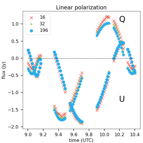
Figure 11: The relative differences between 3 different ipole image resolutions ($16^{2}$, $32^{2}$, $196^{2}$), for all Stokes parameters. In the case of Stokes $\mathcal{Q}$ we have shifted the curve 4 units higher for readability reasons. The bottom right plot shows the full light curves for Stokes $\mathcal{Q}$ and $\mathcal{U}$, since fractional differences can be misleading for values close to zero.

To obtain the results presented in this paper on a reasonable timescale we had to significantly reduce the images resolution in the ray-tracing part of bipole. In what follows, we demonstrate that this does not affect the simulated light curves significantly, especially as far as Stokes $\mathcal{Q},\mathcal{U}$ go. The latter is particularly important for our algorithm which relies on fitting $\mathcal{Q}$ and $\mathcal{U}$ only.

In Fig. 11 we show the relative difference (in percentile) of the light curves using 3 different resolutions ($16^{2}$, $32^{2}$, $196^{2}$) for all Stokes parameters using a random combination of model parameters to create a test light curve that exhibits some structure (in essence, excluding models with constant light curves). Stokes $\mathcal{I}$ exhibits a maximum deviation of $\sim 10\%$ and Stokes $\mathcal{V}$ of $\sim 4\%$. Stokes $\mathcal{Q}$ and $\mathcal{U}$ (see lower panels in Figure 11) peak at $450\%$ but this is rather misleading. Indeed, turning our attention to the bottom right panel we can see that some values lay very close to zero, leading to huge peaks in relative differences. These would be fully absorbed within our error budget.