One–loop Double Copy Relation in String Theory

Abstract

We discuss relations between closed and open string amplitudes at one–loop. While at tree–level these relations are known as Kawai–Lewellen–Tye (KLT) and/or double copy relations, here we investigate how such relations are manifested at one–loop. While there exist examples of one–loop closed string amplitudes that can strikingly be written as sum over squares of one–loop open string amplitudes, generically the one–loop closed string amplitudes assume a form reminiscent from the one–loop doubly copy structure of gravitational amplitudes involving a loop momentum. This double copy structure represents the one–loop generalization of the KLT relations.

I Introduction

The famous Kawai–Lewellen–Tye (KLT) relations express a tree–level closed string amplitude as a weighted sum over squares of tree–level open string amplitudes [1]. Since the lowest mode of the closed superstring is a graviton and that of the open superstring a gluon the aforementioned relation gives rise to a gauge/gravity correspondence linking gravity and gauge amplitudes at the perturbative tree–level. This connection has far reaching consequences after elevating it to the double copy (DC) conjecture [2]. At an abstract level the KLT relations provide a way of computing tree–level closed string world–sheet integrals by reducing them to open string integrals. At the technical level the latter statement means that a complex sphere integral can be expressed in terms of a product of two iterated real integrals. While conjectures based on generalized unitarity for perturbative quantum gravity as a DC structure exist for field theory loop–level [3], only recently a one–loop analog has been found in string theory [4]. In [4] a one–loop extension of the KLT relations has been derived and in this work we elaborate on the underlying DC structure.

II Closed vs. open string amplitudes

Closed string amplitudes are described by integrals over compact Riemann surfaces without boundaries and open string amplitudes are formulated on world–sheets with boundaries. Surfaces with boundaries are obtained from manifolds without boundaries by involution. While closed string vertex positions are integrated over the full manifold those of open strings are integrated along boundaries only. To find relations between closed and open string amplitudes an analytic continuation of each complex closed string coordinate is performed to split the latter into a pair of two real coordinates. The latter describe open string vertex positions located at the boundaries of the underlying world–sheet. At the mathematical level relations between closed and open string amplitudes are subject to holomorphic properties of the string world–sheet and underlying monodromy relations, cf. [5, 6] for tree–level and [7, 8, 9] for one–loop. In fact, while these relations are formulated on surfaces with boundaries, they can be extended to surfaces without boundaries [4].

A. Complex sphere integral

Closed string tree–level $n$–point amplitudes are described by an integral over the moduli space of $n$ marked points on the sphere ${\bf C}$. For $n=4$ we have the integral

$$M^{closed}_{4;0} :=\int_{\bf C}d^{2}z\ |z|^{2\alpha^{\prime}s-2}\ |1-z|^{2\alpha^{\prime}u}$$

$$=\frac{\Gamma(\alpha^{\prime}s)\Gamma(\alpha^{\prime}t)\Gamma(\alpha^{\prime}u)}{\Gamma(1-\alpha^{\prime}s)\Gamma(1-\alpha^{\prime}t)\Gamma(1-\alpha^{\prime}u)},$$ (II.1)

with $s\!+\!t\!+\!u\!=\!0$ and referring to a four–point closed string tree–level amplitude to be specified below. On the other hand, with the corresponding open string disk integrals

$$A^{open}_{4;0} :=\int_{0}^{1}d\xi\ \xi^{\alpha^{\prime}s-1}\ (1-\xi)^{\alpha^{\prime}u}=\frac{\Gamma(\alpha^{\prime}s)\Gamma(\alpha^{\prime}u+1)}{\Gamma(1-\alpha^{\prime}t)},$$ (II.2)

$$\tilde{A}^{open}_{4;0} :=\int_{1}^{\infty}d\eta\ \eta^{\alpha^{\prime}t-1}\ (\eta-1)^{\alpha^{\prime}u}=\frac{\Gamma(\alpha^{\prime}t)\Gamma(\alpha^{\prime}u+1)}{\Gamma(1-\alpha^{\prime}s)},$$ (II.3)

we have:

$$M^{closed}_{4;0}=\sin(\pi\alpha^{\prime}u)\ A^{open}_{4;0}\ \tilde{A}^{open}_{4;0}\ .$$ (II.4)

Actually, (II.2) enters the open superstring subamplitude describing the scattering of four (massless) gluons

$$A^{open}_{4;0}(1,2,3,4)=\frac{t_{8}}{u}\ A_{4;0}^{open}$$ (II.5)

with canonical color ordering $(1,2,3,4)$. With the four external gluon momenta $p_{i}$ (subject to the massless condition $p_{i}^{2}=0$) the three parameters $s,t,u$ refer to the kinematic invariants $s\!=\!2\alpha^{\prime}p_{1}p_{2},t\!=\!2\alpha^{\prime}p_{1}p_{3},u\!=\!2\alpha^{\prime}p_{1}p_{4}$, respectively. Likewise, the four graviton closed superstring amplitude is given by:

$${\cal M}^{closed}_{4;0}=\frac{t_{8}\tilde{t}_{8}}{u^{2}}\ M^{closed}_{4;0}.$$ (II.6)

Thus we have the gravity–gauge relations or four–point KLT relation:

$${\cal M}^{closed}_{4;0}=\sin(\pi\alpha^{\prime}u)\;A^{open}_{4;0}(1,2,3,4)\;\tilde{A}^{open}_{4;0}(1,3,2,4).$$ (II.7)

Similar results can be stated for higher $n$ or massive states:

$$\begin{array}[]{lcl}{\cal M}_{n;0}^{closed}&=&\displaystyle\kappa^{n-2}\ \sum_{\sigma,\rho\in S_{n-3}}A^{open}_{n;0}(1,\sigma(2,3,\ldots,n-2),n-1,n)\\[14.22636pt] &&\displaystyle\times\ \ {\cal S}[\rho|\sigma]_{p_{1}}\ \tilde{A}^{open}_{n;0}(1,\rho(2,3,\ldots,n-2),n,n-1),\end{array}$$ (II.8)

involving the KLT–kernel ${\cal S}[\rho|\sigma]_{p_{0}}$ (intersection matrix). Generically, the latter is defined as a symmetric $k!\times k!$–matrix with its rows and columns corresponding to the orderings $\sigma\equiv\{\sigma(2),\ldots,\rho(k)\}$ and $\rho\equiv\{\rho(1),\ldots,\rho(k)\}$, respectively. For given (cyclic) orderings $\rho,\sigma\in S_{k}$ and a reference momentum $p_{0}$ one defines the KLT kernel as [1, 10, 11]

$${\cal S}[\sigma|\rho]_{p_{0}}:={\cal S}[\,\sigma(1,\ldots,k)\,|\,\rho(1,\ldots,k)\,]_{p_{0}}=\prod_{t=1}^{k}\sin\Bigg{(}\pi\alpha^{\prime}\!\Big{[}p_{0}p_{t_{\sigma}}+\sum_{r<t}p_{r_{\sigma}}p_{t_{\sigma}}\theta(r_{\sigma},t_{\sigma})\Big{]}\Bigg{)},$$ (II.9)

with $j_{\sigma}=\sigma(j)$ and $\theta(r_{\sigma},t_{\sigma})=1$ if the ordering of the legs $r_{\sigma},t_{\sigma}$ is the same in both orderings $\sigma(1,\ldots,k)$ and $\rho(1,\ldots,k)$, and zero otherwise. For the case at hand (II.8) we have $p_{0}=p_{1}$ and $k=n-3$.

B. Complex torus integral

Closed string one–loop $n$–point amplitudes are described by an integral over the moduli space of $n$ marked points on the elliptic curve ${\cal T}$. Let us discuss the one–loop torus integral $(n=2)$

$$\widehat{M}^{closed}_{2;1} :=\int_{\cal T}d^{2}z\;e^{2G^{(1)}(z,\tau)}$$

$$=2\tau_{2}^{\frac{1}{2}}\left|\frac{\theta_{3}\left(2\tau\right)}{\eta^{6}}\right|^{2}+2\tau_{2}^{\frac{1}{2}}\left|\frac{\theta_{2}\left(2\tau\right)}{\eta^{6}}\right|^{2},$$ (II.10)

referring to a specific two–point closed string one–loop amplitude to be specified below. Above, we have introduced the bosonic one–loop Green function

$$G^{(1)}(z,\tau)=\ln\left|\frac{\theta_{1}(z,\tau)}{\theta_{1}^{\prime}(0,\tau)}\right|^{2}-2\pi\frac{(\Im z)^{2}}{\Im\tau}\ ,$$ (II.11)

the odd Riemann theta–function

$$\theta_{1}(z,\tau)=q^{\frac{1}{8}}\sum_{n\in{\bf Z}}(-1)^{n}q^{\frac{1}{2}n(n+1)}\sin[\pi(2n+1)z],$$ (II.12)

and $\eta=q^{1/24}\prod_{n\geq 1}(1-q^{n}),\;q=e^{2\pi i\tau}$. The complex torus coordinate is parameterized as $z=x+\tau y$, with $x,y\in(0,1)$ and the measure $d^{2}z=\tau_{2}dxdy$. Actually, the integral (II.10) describes a one–loop two–point amplitude. In superstring theories the latter and thus mass shifts vanish for massless states, while they do not vanish for massive states, cf. Fig. 1

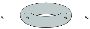
Figure 1: One–loop amplitude with two massive closed strings $q_{i}^{2}\neq 0$.

The two–point amplitude appears as residuum at the first massive level in the factorization of a four–point one–loop amplitude accounting for the mass renormalization in superstring theory [12]. The integral (II.10) computes the mass correction $\delta m^{2}={\cal M}^{closed}_{2;1}$ of the least massive string state in type II superstring theory [12]

$${\cal M}^{closed}_{2;1} =\delta^{(d)}(q_{1}+q_{2})\int\frac{d^{2}\tau}{\tau_{2}}\;\tau_{2}^{-4}$$

$$\times\int_{\cal T}\!d^{2}z\;e^{-\frac{\alpha^{\prime}}{2}q_{1}^{2}G^{(1)}(z,\tau)}\;,$$ (II.13)

subject to momentum conservation $q_{1}+q_{2}=0$ and the on–shell condition for the first massive string state:

$$q_{i}^{2}=-4/\alpha^{\prime}\ \ \ ,\ \ \ i=1,2\ .$$ (II.14)

On the other hand the corresponding real open string planar and non–planar cylinder integrals are

$$A_{2;1}^{p} :=\int_{0}^{1}d\xi\ \frac{\theta_{1}\left(\xi,\tau\right)^{2}}{\eta^{6}}=-\frac{\theta_{2}(2\tau)}{\eta^{6}}\ ,$$ (II.15)

$$A_{2;1}^{np} :=\int_{0}^{1}d\zeta\ \frac{\theta_{4}\left(\zeta,\tau\right)^{2}}{\eta^{6}}=\frac{\theta_{3}(2\tau)}{\eta^{6}},$$ (II.16)

The integrals (II.15) and (II.16) describe the one–loop mass renormalization in $SO(32)$ open superstring theory [13]. Thus, the complex torus integral (II.10) can be cast into the following quadratic form:

$$\widehat{M}_{2;1}^{closed}=2\tau_{2}^{1/2}\;|A_{2;1}^{p}|^{2}+2\tau_{2}^{1/2}\;|A_{2;1}^{np}|^{2}\ .$$ (II.17)

Note, that this is a particular simple DC structure relating a one–loop closed string integral to a sum over squares of open string integrals.

To compute the complex integral (II.10) one starts by expressing the square of the theta–functions (II.12) as

$$e^{2G^{(1)}(z,\tau)} =\frac{1}{4}e^{-4\pi\tau_{2}y^{2}}\sum_{p_{i}\in\{\pm 1\}}\sum_{N_{i},M_{i}\in{\bf Z}}(-1)^{N_{0}+M_{0}}$$

$$\times e^{2\pi izN_{0}}e^{-2\pi i\bar{z}M_{0}}q^{\frac{1}{4}(N_{0}^{2}+N_{1}^{2})}\;\bar{q}^{\frac{1}{4}(M_{0}^{2}+M_{1}^{2})},$$

with the four integers:

$$\begin{array}[]{lcl}N_{0,1}&=&\frac{p_{1}}{2}(2n_{1}+1)\pm\frac{p_{2}}{2}(2n_{2}+1),\\[8.53581pt] M_{0,1}&=&\frac{p_{3}}{2}(2m_{1}+1)\pm\frac{p_{4}}{2}(2m_{2}+1).\end{array}$$ (II.18)

Then, the real $x$–integration gives the level–matching condition:

$$N_{0}=M_{0}.$$ (II.19)

The resulting integer sums over both even and odd $N_{0}$ can be used to extend the real $y$–integration to a Gaussian integral leaving the integer sums with $N_{1},M_{1}$ even or odd subject to the solution (II.19) with $N_{0}$ even or odd, respectfully:

$$\widehat{M}_{2;1}^{closed}=\frac{2\tau_{2}^{1/2}}{|\eta|^{12}}\Bigg{\{}\sum_{N_{1},M_{1}\;even}+\sum_{N_{1},M_{1}\;odd}\Bigg{\}}\;q^{\frac{1}{4}N_{1}^{2}}\bar{q}^{\frac{1}{4}M_{1}^{2}}.$$ (II.20)

Eventually, the above expression leads to (II.10).

Actually, the open string amplitudes (II.15) and (II.16) conspire with one–loop open string monodromy relations [7, 8] as

$$A_{2;1}^{p} =-\tilde{A}_{2;1}^{p}\ ,$$ (II.21)

$$A_{2;1}^{np} =\tilde{A}_{2;1}^{np}$$ (II.22)

giving rise to the additional objects

$$\tilde{A}_{2;1}^{p} :=-\int_{0}^{1}d\zeta\ \frac{\theta_{4}\left(\zeta,\tau\right)^{2}}{\eta^{6}}\ e^{2\pi iz}\;q^{-\tfrac{1}{4}},$$ (II.23)

$$\tilde{A}_{2;1}^{np} :=-\int_{0}^{1}d\xi\ \frac{\theta_{1}\left(\xi,\tau\right)^{2}}{\eta^{6}}\ e^{2\pi iz}\;q^{-\tfrac{1}{4}}\ ,$$ (II.24)

with position dependent phases introduced in [7]. As a consequence we may also write (II.17) as

$$\widehat{M}_{2;1}^{closed}=2\tau_{2}^{1/2}\;|A_{2;1}^{p}|^{2}+2\tau_{2}^{1/2}\;|\tilde{A}_{2;1}^{np}|^{2}\ .$$ (II.25)

It is interesting to note, that the integrand of (II.10) has a ${\bf Z}_{2}$–symmetry $z\rightarrow-z$, i.e. it is sufficient to only integrate over a cylinder world–sheet $\cal C$. Hence, it is instructive to split the torus integral (II.10) into two contributions from cylinder integrals as

$$\widehat{M}^{closed}_{2;1}=\widehat{M}^{p}_{2;1}+\widehat{M}^{np}_{2;1}\ ,$$ (II.26)

with the two cylinder integrals

$$\widehat{M}^{p}_{2;1} =\int_{\cal C}d^{2}z\;e^{2G^{(1)}(z,\tau)}=\frac{1}{2}\;\widehat{M}^{closed}_{2;1}\ ,$$ (II.27)

$$\widehat{M}^{np}_{2;1} =\int_{\cal C}d^{2}z\;e^{2G_{T}^{(1)}(z,\tau)}=\frac{1}{2}\;\widehat{M}^{closed}_{2;1}\ ,$$ (II.28)

which can either be directly computed or by the methods developed in [14]. Above, we have the twisted bosonic one–loop Green function

$$G^{(1)}_{T}(z,\tau)=\ln\left|\frac{\theta_{4}(z,\tau)}{\theta_{1}^{\prime}(0,\tau)}\right|^{2}-2\pi\frac{(\Im z)^{2}}{\Im\tau},$$ (II.29)

with the even Riemann theta–function:

$$\theta_{4}(z,\tau)=\sum_{n\in{\bf Z}}(-1)^{n}q^{\frac{1}{2}n^{2}}\cos(2\pi nz).$$ (II.30)

Hereinafter, we shall use the alternative expression of (II.10) in terms of a loop momentum $\ell$ which manifestly splits the integrand into a holomorphic and anti–holomorphic sector ($d=10$):

$${\cal M}^{closed}_{2;1} =\delta^{(d)}(q_{1}+q_{2})\int_{{\cal F}_{1}}{d^{2}\tau}\int_{-\infty}^{+\infty}d^{d}\ell\;e^{-\pi\alpha^{\prime}\tau_{2}\ell^{2}}$$

$$\times\int_{\cal T}\!d^{2}z\;e^{-i\pi\alpha^{\prime}\ell q_{1}(z-\bar{z})}\left|\frac{\theta_{1}(z,\tau)}{\theta_{1}^{\prime}(0,\tau)}\right|^{4}.$$ (II.31)

In fact, integrating first over the torus coordinate $z$ and performing the sum over $N_{0}$ constrains the loop momentum as:

$$\ell^{\prime}q_{1}=0\ \mbox{with:\ }\ell^{\prime}=\ell+\tfrac{1}{2}q_{1}N_{0}\ .$$ (II.32)

Then, the remaining loop momentum integral decouples and can be performed by introducing spherical Lorentzian coordinates [15] along the axis $q_{1}$:

$$\int_{-\infty}^{+\infty}d^{d}\ell^{\prime}\;e^{-\pi\alpha^{\prime}\tau_{2}\ell^{\prime 2}}\delta^{(d)}(\ell^{\prime}q_{1})=||q_{1}||^{-1}\;(\alpha^{\prime}\tau_{2})^{\frac{1}{2}(1-d)}.$$ (II.33)

Altogether, this yields (II.20) in a different way thereby constraining the loop momentum as (II.32). This result underpins the holomorphic anti–holomorphic factorization of the result (II.17). Furthermore, as it can be anticipated from (II.33) that the constraint (II.32) entails the additional $\tau_{2}^{1/2}$–factors in (II.17) and (II.37).

A similar discussion can be lead for the torus integral:

$$\widehat{\mathfrak{M}}^{closed}_{2;1}:=\int_{\cal T}d^{2}z\;e^{G^{(1)}_{B}(z,\tau)}=2\;\tau_{2}^{\frac{1}{2}}\left|\frac{1}{\eta^{3}}\right|^{2}.$$ (II.34)

Similar to (II.15) and (II.16) we may introduce the following open string integrals:

$${\mathfrak{A}}_{2;1}^{p} :=\int_{0}^{1}d\xi\ \frac{\theta_{1}\left(\xi,\tau\right)}{\eta^{3}}=\frac{2}{\pi}\frac{q^{\tfrac{1}{8}}}{\eta^{3}}\sum_{n\in{{\bf Z}}}(-1)^{n}\frac{q^{\frac{1}{2}(n+1)n}}{2n+1}\ ,$$ (II.35)

$${\mathfrak{A}}_{2;1}^{np} :=\int_{0}^{1}d\zeta\ \frac{\theta_{4}\left(\zeta,\tau\right)}{\eta^{3}}=\frac{1}{\eta^{3}}.$$ (II.36)

Hence, we have the following DC relation:

$$\widehat{\mathfrak{M}}_{2;1}^{closed}=2\;\tau_{2}^{1/2}\;|\mathfrak{A}_{2;1}^{np}|^{2}=2\;\tau_{2}^{1/2}\;|\tilde{\mathfrak{A}}_{2;1}^{np}|^{2}\ .$$ (II.37)

In addition, we have the objects

$$\tilde{\mathfrak{A}}_{2;1}^{p} :=-i\int_{0}^{1}d\zeta\ \frac{\theta_{4}\left(\zeta,\tau\right)}{\eta^{3}}\ e^{\pi iz}\;q^{-\tfrac{1}{8}}$$ (II.38)

$$=\frac{1}{\pi}\frac{q^{-\tfrac{1}{8}}}{\eta^{3}}\sum_{n\in{{\bf Z}}}(-1)^{n}q^{\frac{1}{2}n^{2}}\left(\frac{1}{2n+1}-\frac{1}{2n-1}\right),$$

$$\tilde{\mathfrak{A}}_{2;1}^{np} :=-i\int_{0}^{1}d\xi\ \frac{\theta_{1}\left(\xi,\tau\right)}{\eta^{3}}\ e^{\pi iz}\;q^{-\tfrac{1}{8}}=\frac{1}{\eta^{3}}\ ,$$ (II.39)

which furnish the following open string monodromy relation [7]

$${\mathfrak{A}}_{2;1}^{p}-\tilde{\mathfrak{A}}_{2;1}^{p}=2\;B_{1}\ ,$$ (II.40)

with the following boundary term [7]:

$$B_{1}=\int_{0}^{\tau/2}dz\;\frac{\theta_{1}(z,\tau)}{\eta^{3}}\ .$$ (II.41)

Finally, we shall mention, that expanding the exponential in the integrands of (II.10) and (II.34) yields two–point modular graph functions [16]

$$D_{k}(\tau)=\int_{\cal T}d^{2}z\;G^{(1)}(z,\tau)^{k},$$ (II.42)

e.g. $D_{1}\!=\!0,D_{2}\!=\!E(2,\tau)$, with the non–holomorphic Eisenstein series $E(s,\tau)$. Likewise, expanding the integrand of (II.15) and (II.16) yields two–vertex $B$– and $A$–cycle holomorphic graph functions [17], respectively. Thus, our relations (II.17) and (II.37) are suited to generate relations between elliptic multiple zeta values and their single–valued objects, cf. also [18].

Note, that (II.17) and (II.37) yield KLT squaring identities at string one–loop in the spirit of (II.4). It would be very interesting to find more such examples of complex torus integrals which can be written as squares of open string amplitudes in the spirit of (II.4). For generic $n$ one may expect a splitting of the torus world–sheet into a double of cylinder world-sheets as depicted in Fig. 2

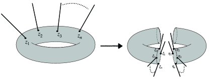
Figure 2: Splitting the torus $n$–point amplitude into two cylinder amplitudes.

On the other hand, one–loop closed string amplitudes with logarithmic branch cuts in their low–energy expansion may not be simple squares of corresponding open string amplitudes. Actually, a generalization of the single complex torus integrals (II.10) and (II.34) represents the Riemann–Wirtinger integral with non–integer powers of $\theta_{1}$ [19]. Its DC structure can be expressed in terms of twisted intersection numbers [20]. In the following we discuss what DC structure to expect in the generic one–loop string case for multiple complex torus integrations.

III String one–loop double copy

In string theory DC structures and numerators have been elaborated at tree–level for the massless case in [21, 22] and for the massive case in [23, 24]. The foundation of these relations are the tree–level KLT relations [1] and only recently a one–loop generalization thereof has been derived [4].

In the following we discuss the one–loop string torus amplitude with $n$ closed oriented strings

$${\cal M}^{closed}_{n;1}(q_{1},\ldots,q_{n})\!=\!\frac{1}{2}g_{c}^{n}\;\delta^{(d)}\!\left(\sum_{r=1}^{n}q_{r}\right)\!\!\int_{{\cal F}_{1}}\!\!\frac{d^{2}\tau}{\tau_{2}}\ M^{closed}_{n;1}\ ,$$ (III.43)

with the integrand

$$M^{closed}_{n;1}=V_{CKG}^{-1}({\cal T})\!\left(\!\int_{{\cal T}}\prod_{s=1}^{n}d^{2}z_{s}\!\right)I(\{z_{s},\bar{z}_{s}\})Q(\{z_{s},\bar{z}_{s}\};\tau),$$ (III.44)

with some doubly–periodic function $Q$ comprising possible kinematical factors. Generically, the latter assumes the form $Q\!=\!\tau_{2}^{1-d/2}Q_{L}(\tau)Q_{R}(\bar{\tau})$. Furthermore, we have the integrand:

$$I(\{z_{s}, \bar{z}_{s}\})=\prod_{1\leq r<s\leq n}\left[\frac{\theta_{1}(z_{s}-z_{r},\tau)}{\theta_{1}^{\prime}(0,\tau)}\right]^{\frac{1}{2}\alpha^{\prime}q_{s}q_{r}}$$ (III.45)

$$\times\left[\frac{\bar{\theta}_{1}(\bar{z}_{s}-\bar{z}_{r},\bar{\tau})}{\bar{\theta}_{1}^{\prime}(0,\bar{\tau})}\right]^{\frac{1}{2}\alpha^{\prime}q_{s}q_{r}}\;\prod_{r,s=1\atop r<s}^{n}e^{-\frac{\pi\alpha^{\prime}}{\tau_{2}}q_{r}q_{s}\Im(z_{r}-z_{s})^{2}}.$$

Note, that due to the lack of holomorphic double periodic functions on the torus we are dealing with quasi–periodic functions (II.29) with non–harmonic contributions. As a consequence there is no holomorphic/anti–holomorphic factorization in contrast to the Virasoro–Shapiro amplitude (II.6). Similar as in (II.31) we introduce the loop momentum $\ell$ to holomorphically factorize the integrand as [25]:

$$\begin{array}[]{lcl}(\alpha^{\prime}\tau_{2})^{-d/2}\ I(\{z_{s},\bar{z}_{s}\})&=&\displaystyle\int_{-\infty}^{\infty}d^{d}\ell\;\exp\Big{\{}-\pi\alpha^{\prime}\tau_{2}\ell^{2}-\pi i\alpha^{\prime}\ell\sum_{r=1}^{n}q_{r}(z_{r}-\bar{z}_{r})\Big{\}}\\ &\times&\displaystyle\prod_{1\leq r<s\leq n}\theta_{1}(z_{s}-z_{r},\tau)^{\frac{1}{2}\alpha^{\prime}q_{s}q_{r}}\ \theta_{1}(\bar{z}_{s}-\bar{z}_{r},\tau)^{\frac{1}{2}\alpha^{\prime}q_{s}q_{r}}.\end{array}$$ (III.46)

After introducing the parameterization $z_{t}=\sigma_{t}^{1}+i\sigma_{t}^{2},\;t=1,\ldots,n$ with $\sigma_{t}^{1}\in(0,1)$ and $\sigma^{2}_{t}\in(-\frac{\tau_{2}}{2},\frac{\tau_{2}}{2})$ for $\Re(\tau)=0$ we may consider some closed contour in the complex $\sigma^{2}_{t}$–plane and express the integration along the real axis $\sigma^{2}_{t}\in(-\frac{\tau_{2}}{2},\frac{\tau_{2}}{2})$ as some integral along the imaginary axis $\sigma_{t}^{2}\in(-i,0)$. This way we have traded each complex integration $z_{s}$ into a pair $\xi_{t},\eta_{t}$ of real integrations [4], with

$$\xi_{t}=\sigma^{1}_{t}+\tilde{\sigma}^{2}_{t}\ \ \ ,\ \ \ \eta_{t}=\sigma^{1}_{t}-\tilde{\sigma}^{2}_{t},$$ (III.47)

at the cost of introducing some splitting function $\Psi$ to be specified below and some phases

$$\Pi_{q}(r,s):=\Pi(\xi_{s},\xi_{r},\eta_{s},\eta_{r};q_{r}q_{s})=e^{\frac{1}{2}\pi i\alpha^{\prime}q_{r}q_{s}(1-\theta[(\xi_{r}-\xi_{s})(\eta_{r}-\eta_{s})])}$$ (III.48)

rendering the integrand of (III.44) to be single–valued along $\xi_{s},\eta_{s}\!\in\!(0,1)$. Eventually, for $\Re(\tau)=0$ the integrand (III.45) becomes [4]:

$$\begin{array}[]{lcl}\displaystyle M^{closed}_{n;1}(q_{1},\ldots,q_{n})&=&\displaystyle\frac{1}{2}\;\delta^{(d)}\Bigg{(}\sum_{i=1}^{n}q_{i}\Bigg{)}\Bigg{(}\frac{i}{2}\Bigg{)}^{n-1}\int_{-\infty}^{\infty}d^{d}\ell\ e^{-\pi\alpha^{\prime}\tau_{2}\ell^{2}}\\[8.53581pt] &\times&\displaystyle\int_{0}^{1}\Bigg{(}\prod_{r=1}^{n-1}d\xi_{r}\Bigg{)}\int_{0}^{1}\Bigg{(}\prod_{r=1}^{n-1}d\eta_{r}\Bigg{)}\Bigg{(}\prod_{t=1}^{n-1}\Psi(\xi_{t},\eta_{t};\ell)\Bigg{)}\mathfrak{I}_{n+2;0}(\ell)\Bigg{(}\prod_{r<s}^{n}\Pi_{q}(r,s)\Bigg{)}\tilde{\mathfrak{I}}_{n+2;0}(\ell).\end{array}$$ (III.49)

The objects in (III.49) represent specific integrands of (planar) one–loop open string amplitudes (with $g_{c}=g_{o}^{2}$):

$$\mathfrak{I}_{n+2;0}(\ell) =g_{o}^{n}\;\Bigg{(}\prod_{r,s=1\atop r<s}^{n}|\theta_{1}(\xi_{s}-\xi_{r},\tau)|^{\frac{1}{2}\alpha^{\prime}q_{s}q_{r}}\Bigg{)}\;e^{-i\pi\alpha^{\prime}\ell\sum\limits_{r=1}^{n}q_{r}\xi_{r}}\;Q_{L}(\tau,\{\xi_{s}\}),$$ (III.50)

$$\tilde{\mathfrak{I}}_{n+2;0}(\ell) =g_{o}^{n}\;\Bigg{(}\prod_{r,s=1\atop r<s}^{n}|\theta_{1}(\eta_{s}-\eta_{r},\tau)|^{\frac{1}{2}\alpha^{\prime}q_{s}q_{r}}\Bigg{)}\;e^{i\pi\alpha^{\prime}\ell\sum\limits_{r=1}^{n}q_{r}\eta_{r}}\;Q_{R}(\overline{\tau},\{\eta_{s}\}).$$ (III.51)

The underlying world–sheet of the expression (III.49) can be interpreted as a non–planar cylinder with a closed string insertion, cf. Fig. 3.

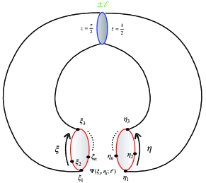
Figure 3: Slicing the torus along the $A$–cycle into one cylinder with a closed string insertion of momentum $\pm\ell$.

More precisely, the one–loop torus is sliced along the $A$–cycle with $2n$ open string positions $\xi_{i}$ and $\eta_{j}$ located along the two boundaries, respectively resulting in a non–planar one–loop cylinder configuration. The details of the cutting procedure is governed by the following splitting function

$$\Psi(\xi_{t},\eta_{t};\ell)=\frac{(1+e^{-\pi i\alpha^{\prime}\ell q_{t}})}{(1-e^{-2\pi i\ell q_{t}})}\;e^{-\pi i\alpha^{\prime}\ell q_{t}\;\theta(\eta_{t}-\xi_{t})}$$ (III.52)

originating from the change of coordinates (III.47) along the two boundaries. The function (III.52) intertwines the real integrations $\xi_{s},\eta_{s}$ with the phase factor $\Pi_{q}$. Furthermore, the splitting function $\Psi$ essentially subjects level matching conditions to the left– and right–movers, which will be evidenced below.

In the large complex structure limit $\tau\rightarrow i\infty$ the closed string becomes a node connecting two degenerating cylinders. In this limit the torus is pinched to a node along the $B$–cycle and the diagram Fig. 3 turns into a product of two disk diagrams each with a single closed string insertion at the node. This limit has thoroughly been worked out in [4]. In particular, the field–theory limit $\alpha^{\prime}\!\rightarrow\!0$ is governed by the large complex structure limit $\tau_{2}\!\rightarrow\!\infty$ of the integrand of (III.43) and exhibits a similar structure than the field–theory DC formula [4]

$${\cal M}^{grav}_{n;1} \simeq\frac{1}{2}\delta^{(d)}\Big{(}\sum\limits_{i=1}^{n}q_{i}\Big{)}\int\frac{d^{d}\ell}{\ell^{2}}$$ (III.53)

$$\sum_{\sigma,\rho\in S_{n-1}}\!\!A_{n+2;0}(+\ell,\sigma(1,\ldots,n-1),n,-\ell)$$

$$\times S[\sigma|\rho]_{\ell}\;\tilde{A}_{n+2;0}(+\ell,\rho(1,\ldots,n-1),-\ell,n),$$

involving the loop momentum $\ell$ and the (off–shell) $n+2$–point tree–level gluon amplitudes in the forward limit

$$A_{n;1}(1,\ldots,n)\!=\!\int\frac{d^{d}\ell}{\ell^{2}}\!\!\!\!\sum_{\gamma\in cyc(1,\ldots,n)}\!\!\!\!\!A_{n+2;0}(+\ell,\gamma(1,\ldots,n),-\ell),$$ (III.54)

with the external momenta $\pm\ell$ [26, 27]. Furthermore, there is the field–theory kernel (II.9), with $S[\sigma|\rho]_{\ell}:=\lim_{\alpha^{\prime}\rightarrow 0}(\pi\alpha^{\prime})^{1-n}{\cal S}[\sigma|\rho]_{\ell}$. In this formulation the loop momentum $\ell$ is identified with a light–like external momentum of a tree–level amplitude $A_{n+2;0}$. The expression (III.53) has formerly been conjectured in [28].

Let us now return to the example (II.10) and its loop momentum description (II.31) [29]. For this case in the general expression (III.44) we have $z_{1}\!=\!z,z_{2}\!=\!0$ and (II.14). Then (III.49) becomes:

$$\begin{array}[]{lcl}\displaystyle M_{2;1}^{closed}(q_{1},q_{2})&=&\displaystyle\frac{1}{4}\frac{i}{2}\!\!\!\sum_{p_{i}\in\{\pm 1\}}\int_{-\infty}^{\infty}d^{d}\ell\;e^{-\pi\alpha^{\prime}\tau_{2}\ell^{2}}\;\sum_{N_{i},M_{i}\in{\bf Z}}(-1)^{N_{0}+M_{0}}q^{\frac{1}{2}(N_{0}^{2}+N_{1}^{2})}\;\bar{q}^{\frac{1}{2}(M_{0}^{2}+M_{1}^{2})}\\[14.22636pt] &\times&\displaystyle\int_{0}^{1}\!\!d\xi\int_{0}^{1}\!\!d\eta\;\Psi(\xi,\eta;\ell)\;e^{2\pi i\xi(N_{0}-\frac{\alpha^{\prime}}{2}\ell q_{1})}e^{-2\pi i\eta(M_{0}-\frac{\alpha^{\prime}}{2}\ell q_{1})}.\end{array}$$ (III.55)

After performing the real $\xi,\eta$–integrations we evidence the imposition of the level–matching condition (II.19):

$$\int_{0}^{1}\!\!d\xi\int_{0}^{1}\!\!d\eta\;\Psi(\xi,\eta;\ell)\;e^{2\pi i\xi(N_{0}-\frac{\alpha^{\prime}}{2}\ell q_{1})}e^{-2\pi i\eta(M_{0}-\frac{\alpha^{\prime}}{2}\ell q_{1})}=-\frac{\delta(M_{0}-N_{0})}{2\pi i(M_{0}-\frac{\alpha^{\prime}}{2}\ell q_{1})}.$$ (III.56)

After shifting the loop momentum by $\ell=\ell^{\prime}-\frac{1}{2}q_{1}M_{0}$ in accord with (II.32) we may cast (III.55) into the following form:

$$M_{2;1}^{closed}=2\int_{-\infty}^{\infty}d^{d}\ell^{\prime}\;\frac{e^{-\pi\alpha^{\prime}\tau_{2}\ell^{\prime 2}}}{2\pi\alpha^{\prime}\ell^{\prime}q_{1}}\;\left(e^{\pi\alpha^{\prime}\ell^{\prime}q_{1}\tau_{2}}-e^{-\pi\alpha^{\prime}\ell^{\prime}q_{1}\tau_{2}}\right)\!\left\{\left|\frac{\theta_{2}(2\tau)}{\eta^{6}}\right|^{2}\!\!\!\sum_{N_{0}\;\mbox{\small even}}e^{\pi\alpha^{\prime}\ell^{\prime}q_{1}\tau_{2}N_{0}}+\left|\frac{\theta_{3}(2\tau)}{\eta^{6}}\right|^{2}\!\!\!\sum_{N_{0}\;\mbox{\small odd}}e^{\pi\alpha^{\prime}\ell^{\prime}q_{1}\tau_{2}N_{0}}\right\}\!.$$ (III.57)

On the other hand, the corresponding expression from (II.31) yields:

$$M_{2;1}^{closed}=2\int_{-\infty}^{\infty}d^{d}\ell^{\prime}\;\frac{e^{-\pi\alpha^{\prime}\tau_{2}\ell^{\prime 2}}}{2\pi\alpha^{\prime}\ell^{\prime}q_{1}}\;\left(e^{2\pi\alpha^{\prime}\ell^{\prime}q_{1}\tau_{2}}-1\right)\left\{\left|\frac{\theta_{2}(2\tau)}{\eta^{6}}\right|^{2}\!\!\!\sum_{N_{0}\;\mbox{\small even}}e^{\pi\alpha^{\prime}\ell^{\prime}q_{1}\tau_{2}N_{0}}+\left|\frac{\theta_{3}(2\tau)}{\eta^{6}}\right|^{2}\!\!\!\sum_{N_{0}\;\mbox{\small odd}}e^{\pi\alpha^{\prime}\ell^{\prime}q_{1}\tau_{2}N_{0}}\right\}.$$ (III.58)

The last two expressions (III.57) and (III.58) involve infinite sums

$$\sum_{N_{0}\;\mbox{\small even}}e^{\pi\alpha^{\prime}\ell^{\prime}q_{1}\tau_{2}N_{0}} =\frac{1}{2}(\pi\tau_{2})^{-1}\;\delta(\alpha^{\prime}\ell q_{1})\;,$$ (III.59)

$$\sum_{N_{0}\;\mbox{\small odd}}e^{\pi\alpha^{\prime}\ell^{\prime}q_{1}\tau_{2}N_{0}} =\frac{1}{2}(\pi\tau_{2})^{-1}\;\delta(\alpha^{\prime}\ell q_{1})\;,$$ (III.60)

and agree subject to the delta–function support (II.32) leading to

$$M_{2;1}^{closed} =2\int_{-\infty}^{\infty}d^{d}\ell^{\prime}\;e^{-\pi\alpha^{\prime}\tau_{2}\ell^{\prime 2}}\ \delta(l^{\prime}q_{1})$$

$$\times\left\{\left|\frac{\theta_{2}(2\tau)}{\eta^{6}}\right|^{2}+\left|\frac{\theta_{3}(2\tau)}{\eta^{6}}\right|^{2}\right\}.$$ (III.61)

This is the result stemming from the direct computation (II.31) and in agreement with (II.10). A similar check can be done for the example (II.34).

For $\Re\tau=0$ our result (III.49) generalizes the tree–level KLT relations to one–loop and it can be applied for both the massless and massive case – with or without supersymmetry. As a consequence in the field–theory limit our relations capitalize solid one–loop gauge–gravity relations including loop–level color kinematics duality. Generalization of (III.49) to $\Re\tau\neq 0$ is very interesting. This task requires extending the analytic continuation of complex vertex operator positions to non–rectangular tori. Complementary, in some recent work the imaginary part of a one–loop string amplitude is computed by considering unitary cuts of the string world–sheet and including massive states [30]. At tree–level there are further relations between closed and open string world–sheet diagrams due to the single–valued projection, cf. for [31] a review. Furthermore, a kind of opposite question is when starting from a single–valued amplitude and asking how the latter can be related to a pair of amplitude expressions with multi–valued coefficients, cf. interesting work [32].

Acknowledgments: I wish to thank Johannes Broedel and Pouria Mazloumi for interesting discussions.

References

• [1] H. Kawai, D. C. Lewellen, and S. H. H. Tye, A Relation Between Tree Amplitudes of Closed and Open Strings, Nucl. Phys. B 269, 1 (1986).
• [2] Z. Bern, J. J. Carrasco, and H. Johansson, New Relations for Gauge-Theory Amplitudes, Phys. Rev. D 78, 085011 (2008), arXiv:0805.3993.
• [3] Z. Bern, J. J. Carrasco, and H. Johansson, Perturbative Quantum Gravity as a Double Copy of Gauge Theory, Phys. Rev. Lett. 105, 061602 (2010), arXiv:1004.0476.
• [4] S. Stieberger, A Relation between One-Loop Amplitudes of Closed and Open Strings (One-Loop KLT Relation), (2022), arXiv:2212.06816.
• [5] S. Stieberger, Open & Closed vs. Pure Open String Disk Amplitudes, (2009), arXiv:0907.2211.
• [6] N. E. J. Bjerrum-Bohr, P. H. Damgaard, and P. Vanhove, Minimal Basis for Gauge Theory Amplitudes, Phys. Rev. Lett. 103, 161602 (2009), arXiv:0907.1425.
• [7] S. Hohenegger and S. Stieberger, Monodromy Relations in Higher-Loop String Amplitudes, Nucl. Phys. B 925, 63 (2017), arXiv:1702.04963.
• [8] P. Tourkine and P. Vanhove, Higher-loop amplitude monodromy relations in string and gauge theory, Phys. Rev. Lett. 117, 211601 (2016), arXiv:1608.01665.
• [9] E. Casali, S. Mizera, and P. Tourkine, Monodromy relations from twisted homology, JHEP 12, 087 (2019), arXiv:1910.08514.
• [10] Z. Bern, L. J. Dixon, M. Perelstein, and J. S. Rozowsky, Multileg one loop gravity amplitudes from gauge theory, Nucl. Phys. B 546, 423 (1999), arXiv:hep-th/9811140.
• [11] N. E. J. Bjerrum-Bohr, P. H. Damgaard, T. Sondergaard, and P. Vanhove, The Momentum Kernel of Gauge and Gravity Theories, JHEP 01, 001 (2011), arXiv:1010.3933.
• [12] N. Marcus, Unitarity and Regularized Divergences in String Amplitudes, Phys. Lett. B 219, 265 (1989).
• [13] H. Yamamoto, One Loop Mass Shifts in O(32) Open Superstring Theory, Prog. Theor. Phys. 79, 189 (1988).
• [14] S. Stieberger, Open & Closed vs. Pure Open String One-Loop Amplitudes, (2021), arXiv:2105.06888.
• [15] G. S. Birman and K. Nomizu, Trigonometry in Lorentzian Geometry, The American Mathematical Monthly 91, 543 (1984).
• [16] M. B. Green, J. G. Russo, and P. Vanhove, Low energy expansion of the four-particle genus-one amplitude in type II superstring theory, JHEP 02, 020 (2008), arXiv:0801.0322.
• [17] J. Broedel, O. Schlotterer, and F. Zerbini, From elliptic multiple zeta values to modular graph functions: open and closed strings at one loop, JHEP 01, 155 (2019), arXiv:1803.00527.
• [18] D. Zagier and F. Zerbini, Genus-zero and genus-one string amplitudes and special multiple zeta values, Commun. Num. Theor. Phys. 14, 413 (2020), arXiv:1906.12339.
• [19] S. Ghazouani and L. Pirio, Moduli spaces of flat tori and elliptic hypergeometric functions, arXiv:1605.02356 (2016).
• [20] Y. Goto, Intersection numbers of twisted homology and cohomology groups associated to the Riemann–Wirtinger integral, International Journal of Mathematics 34, 2350005 (2023).
• [21] C. R. Mafra, O. Schlotterer, and S. Stieberger, Explicit BCJ Numerators from Pure Spinors, JHEP 07, 092 (2011), arXiv:1104.5224.
• [22] J. Broedel, O. Schlotterer, and S. Stieberger, Polylogarithms, Multiple Zeta Values and Superstring Amplitudes, Fortsch. Phys. 61, 812 (2013), arXiv:1304.7267.
• [23] T. Azevedo, M. Chiodaroli, H. Johansson, and O. Schlotterer, Heterotic and bosonic string amplitudes via field theory, JHEP 10, 012 (2018), arXiv:1803.05452.
• [24] D. Lüst, C. Markou, P. Mazloumi, and S. Stieberger, A stringy massive double copy, JHEP 08, 193 (2023), arXiv:2301.07110.
• [25] E. D’Hoker and D. H. Phong, The Geometry of String Perturbation Theory, Rev. Mod. Phys. 60, 917 (1988).
• [26] Y. Geyer, L. Mason, R. Monteiro, and P. Tourkine, Loop Integrands for Scattering Amplitudes from the Riemann Sphere, Phys. Rev. Lett. 115, 121603 (2015), arXiv:1507.00321.
• [27] Y. Geyer, L. Mason, R. Monteiro, and P. Tourkine, One-loop amplitudes on the Riemann sphere, JHEP 03, 114 (2016), arXiv:1511.06315.
• [28] S. He and O. Schlotterer, New Relations for Gauge-Theory and Gravity Amplitudes at Loop Level, Phys. Rev. Lett. 118, 161601 (2017), arXiv:1612.00417.
• [29] We have the relation $\left.M^{closed}_{n;1}=\tau_{2}^{-d/2}\widehat{M}^{closed}_{n;1}\right|_{\Re(\tau)=0}$.
• [30] L. Eberhardt and S. Mizera, Unitarity cuts of the worldsheet, SciPost Phys. 14, 015 (2023), arXiv:2208.12233.
• [31] S. Stieberger, Periods and Superstring Amplitudes, (2016), arXiv:1605.03630.
• [32] K. Baune and J. Broedel, A KLT-like construction for multi-Regge amplitudes, (2023), arXiv:2306.16257.