Accountable Offline Control with (the Minimal Convex Set of) Decision Corpus

1 Introduction

In recent years, offline control that uses pre-collected data to generate control policies has gained attention due to its potential to reduce the costs and risks associated with applying control algorithms in real-world systems (levine2020offline), which are especially advantageous in situations where real-time feedback is challenging or expensive to obtain (kalashnikov2018scalable; jaques2019way; kahn2021badgr; holt2023activeobservingcontrol). However, existing literature has primarily focused on enhancing learning performance, leaving the need for accountable and reliable control policies in offline settings largely unaddressed, particularly for high-stakes, responsibility-sensitive applications.

However, in many critical real-world applications such as healthcare, the challenge is beyond enhancing policy performance. It requires the decisions made by learned policies to be transparent, traceable, and justifiable. Yet those essential properties, summarized as Accountability, are left largely unaddressed by existing literature.

In our context, we use Accountability to indicate the existence of a supportive basis for decision-making. For instance, in tumor treatment using high-risk options like radiotherapy and chemotherapy, the treatment decisions should be based on the successful outcomes experienced by previous patients who share similar conditions and were given the same medication. Another concrete illustrative example is the allocation decisions of ventilator machines. The decision to allocate a ventilator should be accountable, in the way that it juxtaposes the potential consequences of both utilization and non-utilization and provides a reasonable decision on those bases. In those examples, the ability to refer to existing cases that support current decisions can enhance reliability and facilitate reasoning or debugging of the policy. To advance offline control towards real-world responsibility-sensitive applications, five properties are desirable: (P1) controllable conservation: this ensures the policy learning performance by avoiding aggressive extrapolation. (P2) accountability: as underscored by our prior examples, there is a need for a clear basis upon which decisions are made. (P3) suitability for low-data regimes: given the frequent scarcity of high-stake decision data, it’s essential to have methods that perform well with limited data. (P4) adaptability to user specification: this ensures the policy can adjust to changes, like evolving clinical guidelines, allowing for tailored solutions. (P5) flexibility in Strictly Offline Imitation: this property ensures a broader applicability across various scenarios and data availability.

To embody all these properties, we need to venture beyond the current scope of literature focused on conservative offline learning. In our work:

1. Methodologically, we introduce the formal definitions and necessary concepts in accountable decision-making. We propose the Accountable Offline Controller (AOC), which makes decisions according to a decomposition on the basis of the representative existing decision examples.

2. Theoretically, we prove the existence and uniqueness of the decomposition under mild conditions, guiding the design of our algorithms.

3. Practically, we introduce an efficient algorithm that takes all the aforementioned desired properties into consideration and circumvented the computational difficulty.

4. Empirically, we verify and highlight the desired properties of AOC on a variety of offline control tasks, including five simulated continuous control tasks and one real-world healthcare dataset.

2 Preliminaries

POMDP

We develop our work under the general Partially Observable Markov Decision Process (POMDP) setting, denoted as a tuple $(\mathcal{X},\omega,\mathcal{O},\mathcal{A},\mathcal{T},\mathcal{R},\gamma,\rho_{0})$, where $\mathcal{X}\subseteq\mathbb{R}^{d_{x}}$ denotes the underlying $d_{x}$ dimensional state space, $\omega:\mathcal{X}\mapsto\mathcal{O}$ is the emission function that maps the underlying state into a $d_{o}$ dimensional observation $\mathcal{O}\subseteq\mathbb{R}^{d_{o}}$; $\mathcal{A}\subseteq\mathbb{R}^{d_{a}}$ is a $d_{a}$ dimensional action space, transition dynamics $\mathcal{T}:\mathcal{X}\times\mathcal{A}\mapsto\mathcal{X}$ controls the underlying transition between states given actions; and the reward function $\mathcal{R}:\mathcal{X}\mapsto\mathbb{R}$ maps state into a reward scalar; we use $\gamma$ to denote the discount factor and $\rho_{0}$ the initial state distribution. Note that the MDP is the case when $\omega$ is an identical mapping.

Offline Control

Specifically, our work considers the offline learning problem: a logged dataset $\mathcal{D}=\{o^{i}_{t},a^{i}_{t},r^{i}_{t},o^{i}_{t+1}\}^{i=1,...,N}_{t=1,...,T}$ containing $N$ trajectories with length $T$ is collected by rolling out some behavior policies in the POMDP, where $x^{i}_{0}\sim\rho_{0}$ sampled from the initial state distribution and $o^{i}_{0}=\omega(x^{i}_{0})$, $a^{i}_{t}\sim\pi^{i}_{b}$ sampled from unknown behavior policies $\pi^{i}_{b}$. We denote the observational transition history until time $t$ as $h_{t}$, such that $h_{t}=(o_{<t},a_{<t},r_{<t})\in\mathcal{H}\subseteq\mathbb{R}^{(d_{o}+d_{a}+1)\cdot(t-1)}$.

Learning Objective

A policy $\pi:\mathcal{O}\times\mathcal{H}\mapsto\mathcal{A}$ is a function of observational transition history. The learning objective is to find $\pi$ that maximizes the expected cumulative return in the POMDP:

$$\max_{\pi}\mathbb{E}_{\tau\sim\rho_{0},\pi,\mathcal{T}}\left[\gamma^{t}r_{t}\right]$$ (1)

where $\tau\sim\rho_{0},\pi,\mathcal{T}$ means the trajectories $\tau$ is generated by sampling initial state $x_{0}$ from $\rho_{0}$, and action $a$ from $\pi$, such that: $\tau=\{x_{0},o_{0}=\omega(x_{0}),a_{0}=\pi(o_{0},h_{0}=\phi),x_{1}=\mathcal{T}(x_{0},a_{0}),r_{0}=\mathcal{R}(x_{1}),...\}$. A learned belief variable $b_{t}\in\mathbb{R}^{d_{b}}$ can be introduced to represent the underlying state $x_{t}$.

3 Accountable Control with Decision Corpus

3.1 Method Sketh: A Roadmap

The high-level core idea of our work is to introduce an example-based accountable framework for offline decision-making, such that the decision basis can be clear and transparent.

To achieve this, a naive approach would be to leverage the insights of Nearest Neighbors: for each action, this involves finding the most similar transitions in the offline dataset, and estimating the corresponding outcomes. Nonetheless, a pivotal hurdle arises in defining similarity, particularly when taking into account the intricate nature of trajectories, given both the observation space heterogeneity and the inherent temporal structure in decision-making. Compounding such a challenge, another difficulty arises in identifying the most representative examples and integrating the pivotal principle of conservation, which is widely acknowledged to be essential for the success of offline policy learning.

Our proposed method seeks to address those challenges. We start by introducing the basic definitions to support a formal discussion of accountability: in Definition 3.1, we introduce the concept of Decision Corpus.

To address the similarity challenge, we showcase that a nice linear property (Property 3.3) generally exists (Remarks 3.2 & 3.3) when working in the belief space (Definition 3.4). This subsequently leads to a theoretical bound for estimation error (Proposition 3.6);

To address the representative challenge while obeying the principle of conservation, we underscore those examples that span the convex hull (Definition 3.5) and introduce the related optimization objective (Definition 3.6 & 3.7). In a nutshell, the intuition is to use a minimal set of representative training examples to encapsulate test-time decisions. Under mild conditions, we show the solution would exist and be unique (Proposition 3.7).

3.2 Understanding Decision-Making with a Subset of Offline Data

In order to perform accountable decision-making, we construct our approach upon the foundation of the example-based explanation framework (keane2019case; crabbe2021explaining), which motivates us to define the offline decision dataset $\mathcal{D}$ as the Decision Corpus, and introduce the concept of Corpus Subset that is composed of a representative subset of the decision corpus. These corpus subsets will be utilized for comprehending control decisions. Formally:

Definition 3.1 (Corpus Subset).

A Corpus Subset $\mathcal{C}$ is defined as a subset of the decision corpus $\mathcal{D}$, indexed by $[C]:=\{1,2,...,C\}$ — the natural numbers between $1$ and $C$.

$$\mathcal{C}=\left\{(o^{c},a^{c},h^{c},v^{c})\in\mathcal{D}\bigg{|}c\in[C]\right\}.$$ (2)

In the equation above, the transition tuple $(o^{c},a^{c},h^{c},v^{c})$ can be obtained from the decision corpus. We absorb both superscripts ($i$) and subscripts ($t$) to the index ($c$) for the conciseness of notions. Later in our work, we use subscripts $t$ to denote the control time step. The variable $v^{c}\in\mathcal{V}\subseteq\mathbb{R}$ represents a performance metric that is defined based on the user-specified decision objective. e.g., $v^{c}$ may correspond to an ongoing cumulative return, immediate reward, or a risk-sensitive measure.

Our objective is to understand the decision-making process for control time rollouts with the decision corpus. To do this, a naive approach is to reconstruct the control time examples with the corpus subset $(o_{t},a_{t},h_{t})=\sum_{c=1}^{C}w^{c}(o^{c},a^{c},h^{c})$, where $w^{c}\in[0,1]$ and $\sum_{c=1}^{C}w^{c}=1$. Then the corresponding performance measures $v^{c}$ can be used to estimate $v_{t}|a_{t}$ — the control time return of a given decision $a_{t}$. Nonetheless, there are critical issues associated with this straightforward method:

1. Defining a distance metric for the joint observation-action-history space presents a challenge. This is not only due to the fact that various historical observations are defined over different spaces but also because the Euclidean distance fails to capture the structural information effectively.

2. The conversion from the observation-action-history space to the performance measure does not necessarily correspond to a linear mapping: $v_{t}\neq\sum_{c=1}^{C}w^{c}v^{c}$.

To address those difficulties, we propose an alternative approach called Accountable Offline Controller (AOC) that executes traceable offline control leveraging certain examples as decision corpus.

3.3 Linear Belief Learning for Accountable Offline Control

To alleviate the above problems, we first introduce a specific type of belief function $\boldsymbol{b}:\mathcal{O}\times\mathcal{A}\times\mathcal{H}\mapsto\mathcal{B}\subseteq\mathbb{R}^{d_{b}}$, which maps a joint observation-action-history input onto a $d_{b}$-dimensional belief space. [Belief Space Linearity] The performance measure function $\boldsymbol{V}:\mathcal{O}\times\mathcal{A}\times\mathcal{H}\mapsto\mathcal{V}$ can always be decomposed as $\boldsymbol{V}=\boldsymbol{l}\circ\boldsymbol{b}$, where $\boldsymbol{b}:\mathcal{O}\times\mathcal{A}\times\mathcal{H}\mapsto\mathcal{B}\subseteq\mathbb{R}^{d_{b}}$ maps the joint observation-action-history space to a $d_{b}$ dimensional belief variable $b_{t}=\boldsymbol{b}(o_{t},a_{t},h_{t})$ and $\boldsymbol{l}:\mathcal{B}\mapsto\mathcal{V}$ is a linear function that maps the belief $b_{t}$ to an output $\boldsymbol{l}(b_{t})\in\mathcal{V}$.

Remark 3.2.

This property is often the case with prevailing neural network approximators, where the belief state is the last activated layer before the final linear output layer.

Remark 3.3.

The belief mapping function maps a $d_{o}+d_{a}+(d_{o}+d_{a}+1)\cdot(t-1)$ dimensional varied-length input into a fixed-length $d_{b}$ dimensional output. Usually, we have $1=d_{v}<d_{b}\ll d_{o}+d_{a}+(d_{o}+d_{a}+1)\cdot(t-1)$. It is important to highlight that calculating the distance in the belief space is feasible, whereas it is intractable in the joint original space.

Based on Property 3.3, the linear relationship between the belief variable and the performance measure makes belief space a better choice for example-based decision understanding — this is because linearly decomposing the belief space also breaks down the performance measure, hence can guide action selection towards optimizing the performance metric. To be specific, we have

$$v(a_{t}|o_{t},h_{t})=\boldsymbol{l}\circ\boldsymbol{b}(o_{t},a_{t},h_{t})=\boldsymbol{l}\circ\sum_{c=1}^{C}w^{c}\cdot\boldsymbol{b}(o^{c},a^{c},h^{c})=\sum_{c=1}^{C}w^{c}\cdot\boldsymbol{l}\circ\boldsymbol{b}(o^{c},a^{c},h^{c})=\sum_{c=1}^{C}w^{c}\cdot v^{c}$$ (3)

Although we have formally defined of the Corpus Subset, its composition has not been explicitly specified. We will now present the fundamental principles and techniques employed to create a practical Corpus Subset.

3.4 Selection of Corpus Subset

As suggested by Equation (3), if a belief state can be expressed as a linear combination of examples from the offline dataset, the same weights applied to the linear decomposition of the belief space can be utilized to decompose and synthesize the outcome. More formally, we define the convex hull spanned by the image of the Corpus Subset under the mapping function $\boldsymbol{b}$:

Definition 3.4 (Belief Corpus Subset).

A Belief Corpus Subset $\boldsymbol{b}(\mathcal{C})$ is defined by applying the belief function $\boldsymbol{b}$ to the corpus subset $\mathcal{C}$, with the corresponding set of values denoted as $v(\mathcal{C})$:

$$\boldsymbol{b}(\mathcal{C}),v(\mathcal{C})=\left\{b^{c}=\boldsymbol{b}(o^{c},a^{c},h^{c}),v^{c}\bigg{|}(o^{c},a^{c},h^{c},v^{c})\in\mathcal{C}\right\}\subset\mathcal{B}\times\mathcal{V}$$ (4)

Definition 3.5 (Belief Corpus Convex Hull).

The Belief Corpus Convex Hull spanned by a corpus subset $\mathcal{C}$ with the belief corpus $\boldsymbol{b}(\mathcal{C})$ is the convex set

$$\mathcal{C}\mathcal{B}(\mathcal{C})=\left\{\sum_{c=1}^{C}w^{c}b^{c}\bigg{|}w^{c}\in[0,1],b^{c}\in\boldsymbol{b}(\mathcal{C}),\forall c\in[C],\sum_{c=1}^{C}w^{c}=1\right\}$$ (5)

Note that an accurate belief corpus subset decomposition for a specific control time belief value $b_{t}$ may be unattainable when $b_{t}\notin\mathcal{C}\mathcal{B}(\mathcal{C})$. In such situations, the optimal course of action is to identify the element $\tilde{b}_{t}$ within $\mathcal{C}\mathcal{B}(\mathcal{C})$ that provides the closest approximation to $b_{t}$. Denoting the norm in the belief space as $||\cdot||_{\mathcal{B}}$, this equates to minimizing a corpus residual that is defined as the distance from the control time belief to the nearest point within the belief corpus convex hull:

Definition 3.6 (Belief Corpus Residual).

The Belief Corpus Residual given a control time belief variable $b_{t}$ and a belief corpus subset $\mathcal{C}$ is given as

$$r_{\mathcal{C}}(b_{t})=\min_{\tilde{b}_{t}\in\mathcal{C}\mathcal{B}(\mathcal{C})}||b_{t}-\tilde{b}_{t}||_{\mathcal{B}}$$ (6)

In summary, when $b_{t}$ resides within $\mathcal{C}\mathcal{B}(\mathcal{C})$, it can be decomposed using the belief corpus subset according to $b_{t}=\sum_{c=1}^{C}w^{c}b^{c}$. Here, the weights can be understood as representing the similarity and importance in reconstructing the control time belief variable through the belief corpus subset; otherwise, the optimizer of Equation (6) can be employed as a proxy for $b_{t}$. Under such circumstances, the belief corpus residual acts as a gauge for the degree of extrapolation. Given those definitions, we use the following proposition to inform the choice of an appropriate corpus subset. [Estimation Error Bound for $v(a_{t})$, cf. crabbe2021explaining]propositionPROPone Consider the belief variable $b_{t}=\boldsymbol{b}(o_{t},a_{t},h_{t})$ and $\hat{b}$ the optimizer of Equation (6), the estimated value residual between $\boldsymbol{l}(b_{t})$ and $\boldsymbol{l}(\hat{b})$ is controlled by the corpus residual:

$$||\boldsymbol{l}(\hat{b})-\boldsymbol{l}(b_{t})||_{\mathcal{V}}\leq||\boldsymbol{l}||_{\mathrm{op}}\cdot r_{\mathcal{C}}(b_{t})$$ (7)

where $||\cdot||_{\mathcal{V}}$ is a norm on $\mathcal{V}$ and $||\boldsymbol{l}||_{\mathrm{op}}=\inf\left\{\lambda\in\mathbb{R}^{+}:||\boldsymbol{l}(b)||_{\mathcal{V}}\leq\lambda||b||_{\mathcal{B}}\right\}$ is the operator norm for the linear mapping. Proposition 3.6 indicates that minimizing the belief corpus residual also minimizes the estimation error. In order to approximate the belief variables in control time accurately, we propose to use the corpus subset that spans the minimum convex hull in the belief space.

Definition 3.7 (Minimal Hull and Minimal Corpus Subset).

Denoting the corpus subsets whose belief convex hull contains a belief variable $b_{t}$ by

$$\mathcal{C}(b_{t})=\left\{\mathcal{C}\subseteq\mathcal{D}\bigg{|}b_{t}\in\mathcal{C}\mathcal{B}(\mathcal{C})\right\}$$

Among those subsets, the one that contains maximally $d_{b}+1$ examples and has the smallest hyper-volume forms the minimal hull is called the minimal corpus subset (w.r.t. $b_{t}$), denoted by $\tilde{\mathcal{C}}(b_{t})$:

$$\tilde{\mathcal{C}}(b_{t}):=\arg\min_{\mathcal{C}}\int_{\mathcal{C}\mathcal{B}(\mathcal{C})}dV$$

[Existence and Uniqueness]propositionEnU Consider the belief variable $b_{t}=\boldsymbol{b}(o_{t},a_{t},h_{t})$, if $r_{\mathcal{C}}(b_{t})\leq 0$ holds for $\mathcal{C}=\mathcal{D}$, then $\tilde{\mathcal{C}}(b_{t})$ exists and the decomposition on the corresponding minimal convex hull exists and is unique. In this work, we use the corpus subset that constructs the minimal (belief corpus convex) hull to represent the control time belief variable $b_{t}$. Those concepts are illustrated in Figure 1.

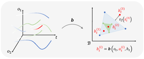
Figure 1: We illustrate the concepts of Corpus Residual and Minimal Hull in a $2$-dim example. The belief function $\boldsymbol{b}$ maps trajectories in the offline dataset (colors of blue and green denote that they may come from different behavior policies) onto the belief space. The control trajectory with different sampled actions at time $t$ can also be mapped to the belief space. Some of those sampled action candidates (e.g., $a_{t}^{(1)},a_{t}^{(2)}$) can be well-supported by a corpus subset, while in another case ($a_{t}^{(3)}$) the corpus residual manifests the extrapolation error. Among the three plotted beliefs generated by candidate actions, $b_{t}^{(3)}$ is out of the convex hulls that can be spanned by any decision corpus, $b_{t}^{(2)}$ has the minimal corpus (green shaded area), $b_{t}^{(1)},b_{t}^{(2)}$ are also in a larger corpus hull (blue shaded area) but it is not ideal.

3.5 Accountable Offline Control with Belief Corpus

Given the linear relationship between the variables $v$ and $b$, for a specific action $a_{t}$, we can estimate the corresponding $\hat{v}(a_{t})=\boldsymbol{l}(\hat{b})=\sum_{c=1}^{C}w^{c}v^{c}$, where $o_{t}$ and $h_{t}$ are the control time observation and transition history respectively. Applying an arg-max type of operator to the above value estimator, we are able to select the action with the highest value that is supported by the belief corpus:

$$\pi_{\mathrm{AOC}}(o_{t},h_{t})=\arg\max_{a_{t}}\hat{v}(a_{t}),$$ (8)

Flexibility of the Measurement Function: Plug-and-Play.

As discussed earlier, the choice of measurement function $\mathbf{V}$ depends on the objective of policy learning. For the low-dimensional tasks, we can instantiate $\mathbf{V}$ using the Monte Carlo estimation of the cumulative return: $v^{c}=\sum_{t=t_{c}}^{T}\gamma^{t-t_{c}}r_{t}$, as the most straightforward choice in control tasks; for higher-dimensional tasks, the measurement metric can be the learned Q-value function; for other applications like when safety-constraints are also taken into consideration, the measurement function can be adapted accordingly.

3.6 Optimization Procedure

The optimization process in our proposed AOC method involves three main steps: optimizing the belief function and linear mapping, reconstructing the belief during control time rollout, and performing sampling-based optimization on the action space. In this section, we detail each of these steps along with corresponding optimization objectives. First, the belief function $\boldsymbol{b}$ and the linear mapping $\boldsymbol{l}$ are learned by minimizing the difference between the predicted performance measure and the actual value $v$ from the dataset $\mathcal{D}$:

$$\small\boldsymbol{b},\boldsymbol{l}=\arg\min_{\boldsymbol{b},\boldsymbol{l}}\mathbb{E}_{(o,a,h,v)\in\mathcal{D}}\left(v-\boldsymbol{l}\circ\boldsymbol{b}(o,a,h)\right)^{2}$$ (9)

Next, with the observation $o_{t}$ and trace $h_{t}$, any candidate action $a_{t}$ corresponds to a belief $b_{t}=\boldsymbol{b}(o_{t},a_{t},h_{t})$, which can be reconstructed by the minimal corpus subset $\tilde{\mathcal{C}}(b_{t})$, according to:

$$\small w^{c}=\arg\min_{w^{c}}||\sum_{c=1}^{C}w^{c}\boldsymbol{b}(o^{c},a^{c},h^{c})-b_{t}||,~{}~{}\mathrm{s.t.}~{}~{}\sum_{c=1}^{C}w^{c}=1,~{}~{}(o^{c},a^{c},h^{c})\in\tilde{\mathcal{C}}(b_{t})$$ (10)

Then the value of action $a_{t}$ can be estimated by $\hat{v}(a_{t}|o_{t},h_{t})=\sum_{c=1}^{C}w^{c}v^{c}$. Finally, we perform a sampling-based optimization on the action space, with the corpus residual taken into consideration for the pursuance of conservation. For each control step, we uniformly sample $K$ actions in the action space ${a^{(k)}{t}}\sim U(\mathcal{A})$ and then search for the action that corresponds to the maximal performance measure while constraining the belief corpus residual to be smaller than a threshold $\epsilon\geq 0$:

$$\small\pi_{\mathrm{AOC}}(o_{t},h_{t})=\arg\max_{a_{t}\in\{a^{(k)}_{t}\}}\sum_{c=1}^{C}w^{c}v^{c},\quad\mathrm{s.t.}~{}~{}~{}r_{\mathcal{C}}(\boldsymbol{b}(o_{t},a_{t},h_{t}))\leq\epsilon$$ (11)

The complete optimization procedure is detailed in Algorithm 1.

Algorithm 1 The Accountable Offline Controller

  Input

       Bached Dataset $\mathcal{D}=\{o^{i}_{t},a^{i}_{t},r^{i}_{t},o^{i}_{t+1}\}^{i=1,...,N}_{t=1,...,T}$, control time observation $o_{t}$, control history $h_{t}$. Hyper-parameters: $K$ for the number of candidate actions, $\epsilon$ for the threshold.

  Output

       Accountable action $a_{t}$ for control.

  $\#$ 1. Optimize belief function $\boldsymbol{b}$ and linear mapping $\boldsymbol{l}$ according to Equation (9).

  $\#$ 2. Sample $K$ candidate actions uniformly in the action space: $a^{k}_{t}\sim U(\mathcal{A}),k\in[K]$.

  $\#$ 3. Find the minimal hulls $\tilde{\mathcal{C}}(b_{t})$ for each action, based on $\boldsymbol{b}$ and $b_{t}=\boldsymbol{b}(o_{t},a^{k}_{t},h_{t})$.

  $\#$ 4. Minimize corpus residuals for each action candidate $a^{k}_{t}$ according to Equation (10).

  $\#$ 5. Estimate the value of action $a_{t}$ by $\hat{v}(a_{t}|o_{t},h_{t})=\sum_{c=1}^{C}w^{c}v^{c}$

  $\#$ 6. Outputs the candidate action that has the highest estimated value according to Equation (11).

4 Related Work

Table 1: AOC is distinct as it satisfies 5 desired properties mentioned earlier: (P1) Conservation: AOC seeks the best potential action in the belief convex hull, such that the estimations of decision outcomes are interpolated, avoiding aggressive extrapolation that is harmful in offline control (fujimoto2019off); (P2) Accountability: the decision-making process is supported by a corpus subset from the offline dataset, hence all the decisions are traceable; (P3) Low-Data Requirement: it works in the low-data regime; (P4) Adaptivity: the control behavior of AOC can be adjusted according to additional constraints as clinical guidelines without modification or re-training; (P5) Reward-Free: AOC can be extended to the strictly offline imitation setting where rewards are unavailable.

Method / Property	Conservation	Accountable	Low-Data	Adaptive	Reward-Free	Examples
Q-Learning	✓	✗	✓	✗	✗	(fujimoto2019off; kumar2019stabilizing; peng2019advantage; agarwal2020optimistic; kumar2020conservative; an2021uncertainty; fujimoto2021minimalist; yang2022rorl; nikulin2023anti)
Episodic Control	✗	✗	✓	✗	✗	(blundell2016model; pritzel2017neural; lin2018episodic)
Nearest Neighbor	✗	✓	✗	✓	✓	(shah2018q; mansimov2018simple)
Model-Based RL	✗	✗	✗	✓	✗	(kidambi2020morel; yu2020mopo; williams2016aggressive)
Behavior Clone	✗	✗	✗	✗	✓	(pomerleau1988alvinn)
AOC	✓	✓	✓	✓	✓	Ours

We review related literature and contrast their difference in Table 1. Due to constraints on space, we have included comprehensive discussions on related work in Appendix LABEL:appdx:extend_related_work. Our proposed method stands out due to its unique attributes: It incorporates properties of accountability, built-in conservation for offline learning, adaptation to preferences or guidelines, is suitable for the low-data regime, and is compatible with the strictly offline imitation learning setting where the reward signal is not recorded in the dataset.

5 Experiments

Environments and Set-ups

In this section, we present empirical evidence of the properties of our proposed method in a variety of environments. These environments include (1) control benchmarks that simulate POMDP and heterogeneous outcomes in healthcare, (2) a continuous navigation task that allows for the visualization of properties, and (3) a real-world healthcare dataset from Ward (alaa2017personalized) that showcases the potential of AOC for deployment in high-stakes, real-world tasks.

In Section 5.1, we benchmark the performance of AOC on the classic control benchmark, contrasting it with other algorithms and highlighting (P1-P3). In Section 5.2, Section 5.3, and Section 5.4 we individually highlight properties (P1),(P2),(P4). Subsequently, in Section 5.5, we apply AOC to a real-world dataset, highlighting its ability to perform accountable, high-quality decision-making under the strictly offline imitation setting (P1-P5). Finally, Section 5.6 provides additional empirical evidence supporting our intuitions and extensive stress tests of AOC.

5.1 (P1-P3): Accountable Offline Control in the Low-Data Regime

Experiment Setting

Our initial experiment employs a synthetic task emulating the healthcare setting, simultaneously allowing for flexibility in stress testing the algorithms.

We adapt our environment, Pendulum-Het, from the classic Pendulum control task involving system stabilization. Heterogeneous outcomes in healthcare contexts are portrayed through varied dynamics governing the data generation process. Data generation process details can be found in Appendix C.1. Taking heterogeneous potential outcomes and partial observability into consideration, the Pendulum-Het task is significantly more challenging than the classical counterpart.

We compare AOC with the nearest-neighbor controller (1NN) (shah2018q) and its variant that using $k$ neighbors (kNN), model-based RL with Mode Predictive Control (MPC) (williams2016aggressive), model-free RL (MFRL) (fujimoto2018addressing), and behavior clone (BC) (pomerleau1988alvinn). Our implementation for those baseline algorithms is based on open-sourced codebases, with details elaborated in Appendix LABEL:appdx:baseline_impl. We change the size of the dataset to showcase the performance difference of various methods under different settings. The Low-Data denotes settings with $100000$ transition steps, Mid-Data denotes settings with $300000$ transition steps, Rich-Data denotes settings with $600000$ transition steps.

Results

We compare AOC against baseline methods in Table 2. AOC achieves the highest average cumulative score among the accountable methods and is comparable with the best black-box controller. In experiments, we find increasing the number of offline training examples does not improve the performance of MFRL due to stability issues. Detailed discussions can be found in Appendix LABEL:appdx:ql_baseline.

Table 2: Results on the Heterogeneous Pendulum dataset. The cumulative reward of each method is reported. Experiments are repeated with $8$ seeds. Higher is better.

Task	Low-Data	Mid-Data	Rich-Data
AOC	$\mathbf{-1.39\pm 1.39}$	$\mathbf{-1.25\pm 0.40}$	$\mathbf{-0.6\pm 0.08}$
kNN	$-849.45\pm 91.23$	$-670.51\pm 321.09$	$-645.72\pm 220.33$
1NN	$-557.07\pm 256.64$	$-690.49\pm 152.59$	$-512.71\pm 131.2$
BC	$-422.77\pm 409.51$	$-225.32\pm 340.83$	$-126.74\pm 280.73$
MFRL	$-4.1\pm 2.76$	$-11.95\pm 4.68$	$-15.27\pm 6.46$
MPC	$\mathbf{-1.5\pm 0.43}$	$\mathbf{-1.34\pm 0.15}$	$-1.41\pm 0.26$
Data-Avg-Return	$-307.81\pm 387.53$	$-245.54\pm 338.65$	$-208.81\pm 272.84$

Take-Away: As an accountable algorithm, AOC performs on par with state-of-the-art black-box learning algorithms. Particularly in the POMDP task, wherein data originates from heterogeneous systems, AOC demonstrates robustness across diverse data availability conditions.

5.2 (P1): Avoid Aggressive Extrapolation with the Minimal Hull and Minimized Residual

Experiment Setting

In Equation (11), our arg-max operator includes two adjustable hyperparameters: the number of uniformly sampled actions and the threshold. In this section, we demonstrate how these hyperparameters can be unified and easily determined.

The consideration of sample size primarily represents a balance between optimization precision and computational cost — although such cost can be minimized by working with modern computational platforms through parallelization. On the other hand, selecting an appropriate value for $\epsilon$ might initially seem complex, as the residual’s magnitude should depend on the learned belief space.

In our implementation, we employ a quantile number to filter out sampled actions whose corresponding corpus residuals exceed a certain population quantile. For instance, when $\epsilon=0.3$ with a sample size of $100$, only the top $30\%$ of actions with the smallest residuals are considered in the arg-max operator in Equation (11). The remaining number of actions is referred to as the effective action size. This section presents results for the Pendulum-Het environment, while additional qualitative and quantitative results on the conservation are available in Appendix LABEL:sec:exp_conservation. Intuitively, using a larger sampling size will improve the performance, at a sub-linear cost of computational expenses, and using a smaller quantile number will make the behavior more conservative. That said, using a small quantile number may not be always good, as it also decreases the effective action size. The golden rule is to use larger sampling size and smaller quantile threshold.

Results

r4.9cm The $\epsilon$ in Equation (11) controls the conservation tendency of the control time behaviors. $\epsilon$ (quantile) Performance $0.3$ $-2.05\pm 0.45$ $0.5$ $-1.25\pm 0.40$ $0.9$ $-503.39\pm 301.60$ $1.0$ $-853.29\pm 138.43$ Table 5.2 exhibits the results. Our experiments highlight the significance of this filtering mechanism: removal or weakening of this mechanism, through a larger quantile number that filters fewer actions, leads to aggressive extrapolation and subsequently, markedly deteriorated performance. This is because the decisions made by AOC in those cases cannot be well supported by the minimal convex hull, introducing substantial epistemic uncertainty in value estimation.

Conversely, using a smaller quantile number yields a reduced effective action size, which subsequently decreases optimization accuracy and leads to a minor performance drop. Hence when computational resources allow, utilizing a larger sample size and a smaller quantile number can stimulate more conservative behavior from AOC. In all experiments reported in Section 5.1, we find a sample size of $100$ and $\epsilon=0.5$ generally work well.

Take-Away: AOC is designed for offline control tasks by adhering to the principle of conservative estimation. The $\epsilon$ hyperparameter, introduced for conservative estimation, can be conveniently determined by incorporating it into the choice of an effective action size.

5.3 (P2): Accountable Offline Control by Tracking Reference Examples

Experiment Setting

r6.0cm Left: the Maze; Right: trajectories generated by $4$ experts for different tasks. In healthcare, the treatments suggested by the clinician during different phases can be based on different patients, and those treatments may even be given by different clinicians according to their expertise. In this section, we highlight the accountability of AOC within a Continuous Maze task. Such a task involves the synthesis of decisions from multiple experts to achieve targeted goals. It resembles the healthcare example above and is ideal for visualizing the concept of accountability.

Figure 5.3 displays the map, tasks, and expert trajectories within a 16x16 Maze environment. This environment accommodates continuous state and action spaces. We gathered trajectories from $4$ agents, each of which is near-optimal for a distinct navigation task:
① agent $\pi_{1}$ starts at position $(0,0)$ and targets position $(8,16)$. Trajectories of $\pi_{1}$ are marked in blue. ② agent $\pi_{2}$ starts at position $(0,0)$ and targets position $(8,8)$. Trajectories of $\pi_{2}$ are marked in orange. ③ agent $\pi_{3}$ starts at position $(8,16)$ and aims position $(16,0)$. Trajectories of $\pi_{3}$ are marked in green. ④ agent $\pi_{4}$ starts at position $(8,8)$ and targets position $(16,0)$. Trajectories of $\pi_{4}$ are marked in red.

We generate 250 trajectories for each of the $4$ agents, creating the offline dataset. The control task initiates at position $(0,0)$, with the goal situated at $(16,0)$ — requires a fusion of expertise in the dataset to finish. To complete the task, an agent could potentially learn to replicate $\pi_{1}$, followed by adopting $\pi_{3}$’s strategy. Alternatively, it could replicate $\pi_{2}$ before adopting $\pi_{4}$’s approach.

Results

r7.8cm Visualize Accountability. The upper colors display the components of the corpus subset at different x-positions. In this experiment, we employ AOC to solve the task and visualize the composition of the corpus subset at each decision step in Figure 5.3. In the initial stages, the corpus subset may comprise a blend of trajectories from $\pi_{1}$ and $\pi_{2}$. Subsequently, AOC selects one of the two potential solutions at random, as reflected in the chosen reference corpus subsets. Upon crossing the central gates on the x-axis, AOC’s decisions become reliant on either $\pi_{3}$ or $\pi_{4}$, persisting until the final steps, when the corpus subsets can again be a mixture of the overlapped trajectories.

Take-Away: AOC’s decision-making process exhibits strong accountability, as the corpus subset can be tracked at every decision-making step. This is evidenced by AOC’s successful completion of a multi-stage Maze task, wherein it effectively learns from mixed trajectories generated by multiple policies at differing stages.

5.4 (P4): Flexible Offline Control under User Specification

Experiment Setting

Given the tractable nature of AOC’s decision-making process, the agent’s behavior can be finely tuned. One practical way of modifying these decisions is to adjust the reference dataset, which potentially contributes to the construction of the corpus subset. In this section, we perform experiments in the Continuous Maze environment with the same offline dataset described in Section 5.3. We modify the sampling rate of trajectories generated by $\pi_{1}$ and experiment with both re-sampling and sub-sampling strategies, using sample rates ranging from $[\times 4,\times 3,\times 2,\times 1,\times 0.75,\times 0.5,\times 0.25]$. In the re-sampling experiments (sample rates larger than $1$), we repeat trajectories produced by $\pi_{1}$ to augment their likelihood of selection as part of the corpus subset. In contrast, the sub-sampling experiments partially omit trajectories from $\pi_{1}$ to reduce their probability of selection. In each setting, 100 control trajectories are generated.

Results

r5.5cm The behavior of AOC can be controlled by re-sampling or sub-sampling the offline dataset. Figure 5.4 shows the results: the success rate (Succ. Rate) quantifies the quality of control time behaviors, while the remaining two curves denote the percentage of control time trajectories that accomplish the task by either following either $\pi_{1}$ - $\pi_{3}$ (passing the upper gate) or $\pi_{2}$ - $\pi_{4}$ (passing the lower gate). The behavior of AOC is influenced by the sampling rate. Utilizing a high sampling rate for the trajectories generated by $\pi_{1}$ often leads to the selection of the solution that traverses the upper gate. As the sampling rate diminishes, AOC’s behavior begins to be dominated by the alternative strategy. In both re-sampling and sub-sampling strategies, the success rate of attaining the goal remains consistently high. We provide further visualizations of the learned policies under various sampling rates in Appendix LABEL:appdx:more_visual_adapt.

Take-Away: The control time behavior of AOC can be manipulated by adjusting the proportions of behaviors within the offline dataset. Both re-sampling and sub-sampling strategies prove equally effective in our experiments where multiple high-performing solutions are available.

5.5 (P1-P5): Real-World Dataset: The Strictly Batch Imitation Setting in Healthcare

Experiment Setting

We experiment with the Ward dataset (alaa2017personalized) that is publicly available with (chan2021medkit). The dataset contains treatment information for more than $6000$ patients who received care on the general medicine floor at a large medical center in California. These patients were diagnosed with a range of ailments, such as pneumonia, sepsis, and fevers, and were generally in stable condition. The measurements recorded included standard vital signs, like blood pressure and pulse, as well as lab test results. In total, there were $8$ static observations and $35$ temporal observations that captured the dynamics of the patient’s conditions. The action space was restricted to a choice of a binary action pertaining to the use of an oxygen therapy device. In the healthcare setting, treatment decisions are given by domain experts and the objective of policy learning is to mimic those expert behaviors through imitation. However, as interaction with the environment is strictly prohibited, the learning and evaluation of policies should be conducted in a strictly offline manner. The dataset is split into $10:1$ training and testing sets and the test set accuracy is used as the performance metric.

We benchmark the variant of AOC tailored for the strictly batch imitation setting, dubbed as ABC — as an abbreviation for Accountable Behavior Clone — against three baselines: (1) behavior cloning with a linear model (BC-LR), which serves as a transparent baseline in the offline imitation setting; (2) behavior cloning with a neural network policy class (BC-MLP), which represents the level of performance achievable by black-box models in such contexts; and (3) the k-nearest neighbor controller (kNN) as an additional accountable baseline.

Results

r5.7cm Results on the Ward dataset. ABC is able to perform accountable imitation under the strict offline setting with high performance comparable with the black-box models. The results of kNN with various choices of $k$ in the experiments, alongside a comparison with ABC using the same number of examples in the corpus subset, are presented in Figure 5.5. Shaded areas in the figure denote the variance across $10$ runs.

Operating as an accountable policy under the offline imitation setting, ABC achieves performance similar to that of behavior cloning methods utilizing black-box models. Meanwhile, other baselines face challenges in striking a balance between transparency and performance.

Furthermore, we visualize the corpus subset supporting control time decisions in a $2$-dimensional belief space to illustrate the accountability. We demonstrate the differences in the decision boundary where predictions are more challenging. In such cases, the decision supports of kNN rely on extrapolation and have no idea of the potential risk of erroneous prediction, while the heterogeneity in ABC’s minimal convex hull reflects the risk. We provide a more detailed discussion in Appendix LABEL:appdx:visualize_ward_patients.

Take-Away: The variant of AOC, dubbed as ABC, is well-suited for the strictly batch imitation setting, enabling accountable policy learning. While other baseline methods in this context struggle to balance transparency and policy performance, ABC achieves comparable performance with black-box models while maintaining accountability.

5.6 Additional Empirical Studies

To further verify our intuitions and stress test AOC, we provide additional empirical analysis in Appendix LABEL:appdx:additional_exps. Specifically, we analyze the trade-off between accountability and performance in Appendix LABEL:sec:exp_5.3; we visualize the controllable conservation in Appendix LABEL:sec:exp_conservation; we benchmark AOC on another benchmark for the general interests of the RL community in Appendix LABEL:exp:lunarlander; and show how to combine AOC with black-box sampler in Appendix LABEL:exp:blackboxsampler; Finally, we show AOC can detect control time OOD examples in Appendix LABEL:appdx:ood.

6 Conclusion

In conclusion, this study presents the Accountable Offline Controller (AOC) as a solution for offline control in responsibility-sensitive applications. AOC possesses five essential properties that make it particularly suitable for tasks where traceability and trust are paramount: ensures accountability through offline decision data, thrives in low-data environments, exhibits conservative behavior in offline contexts, can be easily adapted to user specifications, and demonstrates flexibility in strictly offline imitation learning settings. Results from multiple offline control tasks, including a real-world healthcare dataset, underscore the potential of AOC in enhancing trust and accountability in control systems, paving the way for its widespread adoption in real-world applications.

Acknoledgement

HS acknowledges and thanks the funding from the Office of Naval Research (ONR). HS would thank Jonathan Crabbe for his inspiration and encouragement in exploring this idea in a group meeting. We thank Jonathan Crabbe for reviewing our manuscript and providing insightful comments and suggestions for improving the paper. We thank all anonymous reviewers, ACs, SACs, and PCs for their efforts and time in the reviewing process and in improving our paper. This work is done with the warm support from the van der Schaar Lab members.

Appendix A Missing Proof

Appendix B Implementation Details

Appendix C Additional Experiment Details

C.1 Data Generation Process: Heterogeneous Pendulum

C.2 Q-Learning Baseline

Our implementation of the Q-learning baseline leverages the twin-delayed techniques (fujimoto2018addressing) to stabilize training. We find that Q-learning requires a large batch size (i.e., $10240$) and many optimization epochs to converge. In the experiment settings with more offline data, the convergence becomes even harder: the rich-data regime containing $6\times$ more data takes $6\times$ more training epochs to converge. And the converged performance is always with high vibration, leading to a worse performance.

Learning curves are shown in Figure 2, experiments are done with $8$ seeds and both averaged learning curves and individual curves are plotted.

Figure 2: Q-Learning learning curves.