Deep Reinforcement Learning for Autonomous Cyber Operations: A Survey

Abstract

The rapid increase in the number of cyber-attacks in recent years raises the need for principled methods for defending networks against malicious actors. Deep reinforcement learning (DRL) has emerged as a promising approach for mitigating these attacks. However, while DRL has shown much potential for cyber defence, numerous challenges must be overcome before DRL can be applied to autonomous cyber operations (ACO) at scale. Principled methods are required for environments that confront learners with very high-dimensional state spaces, large multi-discrete action spaces, and adversarial learning. Recent works have reported success in solving these problems individually. There have also been impressive engineering efforts towards solving all three for real-time strategy games. However, applying DRL to the full ACO problem remains an open challenge. Here, we survey the relevant DRL literature and conceptualize an idealised ACO-DRL agent. We provide: i.) A summary of the domain properties that define the ACO problem; ii.) A comprehensive evaluation of the extent to which domains used for benchmarking DRL approaches are comparable to ACO; iii.) An overview of state-of-the-art approaches for scaling DRL to domains that confront learners with the curse of dimensionality, and; iv.) A survey and critique of current methods for limiting the exploitability of agents within adversarial settings from the perspective of ACO. We conclude with open research questions that we hope will motivate future directions for researchers and practitioners working on ACO.

1 Introduction

The rapid increase in the number of cyber-attacks in recent years has raised the need for responsive, adaptive, and scalable autonomous cyber operations (ACO) [9596578, albahar2019cyber]. Adaptive solutions are desirable due to cyber-criminals increasingly showing an ability to evade conventional security systems, which often lack the ability to detect new types of attacks [9277523]. The ACO problem can be formulated as an adversarial game involving a Blue agent tasked with defending cyber resources from a Red attacker [baillie2020cyborg]. Deep reinforcement learning (DRL) has been identified as a suitable machine learning (ML) paradigm to apply to ACO [adawadkar2022cyber, li2019reinforcement, liu2020deep]. However, current out of the box DRL solutions do not scale well to many real world scenarios. This is primarily due to ACO lying at the intersection of three open problem areas for DRL, namely: i.) The efficient processing and exploration of vast high-dimensional state spaces [abel2016exploratory]; ii.) Large combinatorial action spaces, and; iii.) Minimizing the exploitability of DRL agents in adversarial games [gleave2019adversarial] (see fig:aco_requirements).

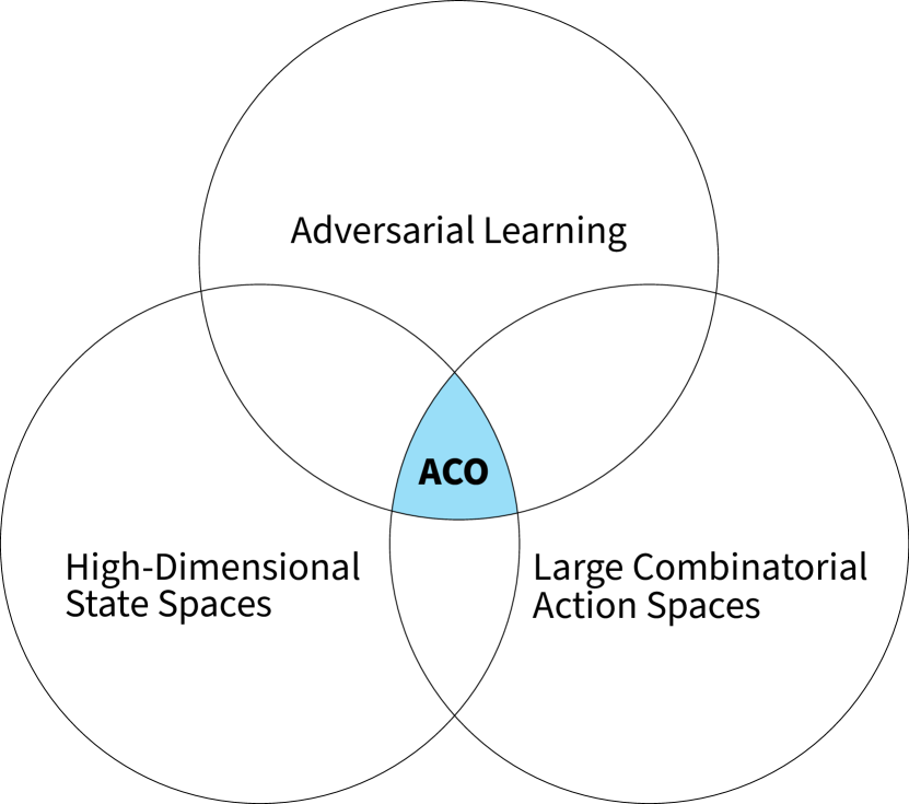
Figure 1: Three challenges that an idealised DRL-ACO agent must conquer.

The DRL literature features a plethora of efforts addressing the above challenges individually. Here, we survey these efforts and define an idealised DRL agent for ACO. This survey provides an overview of the current state of the field, defines long term objectives, and poses research questions for DRL practitioners and ACO researchers to dig their teeth into.

Our contributions can be summarised as follows:

1.) To enable an extensive evaluation of future DRL-ACO approaches, we provide an overview of ACO benchmarking environments, as well as environments found within the DRL literature that confront learners with comparable challenges.

2.) We identify suitable methods for addressing the curse of dimensionality for ACO. This includes a summary of approaches for state-abstraction, efficient exploration and mitigating catastrophic forgetting, as well as a critical evaluation of high-dimensional action approaches.

3.) We formally define the ACO problem from the perspective of adversarial learning. Even within simple adversarial games, finding (near) optimal policies is non-trivial. We therefore review principled methods for limiting exploitability, and map out paths towards scaling these approaches to the full ACO challenge.

2 Related Work

A number of surveys have been conducted in recent years that provide an overview of the different types of cyber attacks (e.g., intrusion, spam, and malware) and the ML methodologies that have been applied in response [9277523, li2018cyber, reda2021taxonomy, liu2019machine, thiyagarajan2020review]. Given that ML methods themselves are susceptible to adversarial attacks, there have also been efforts towards assessing the risk posed by adversarial learning techniques for cyber security [duddu2018survey, rosenberg2021adversarial]. However, while these works evaluate existing threats to ML models in general (e.g., white-box attacks [moosavi2016deepfool] and model poisoning attacks [kloft2010online]), our survey focuses on the adversarial learning process for DRL agents within ACO, desirable solution concepts, and a critical evaluation of existing techniques towards limiting exploitability.

[9596578] surveyed the DRL for cyber security literature, providing an overview of works where DRL-based security methods were applied to cyber–physical systems, autonomous intrusion detection techniques, and multiagent DRL-based game theory simulations for defence strategies against cyber-attacks. In contrast, our work focuses on generation after next solutions; we capture the challenges posed by the ACO problem at scale and survey the DRL literature for suitable methods designed to address these challenges separately, providing the building blocks for an idealised ACO-DRL agent. Such an agent will require a suitable evaluation environment. While there have been efforts towards evaluating cyber security datasets [8258167, kilincer2021machine, 9277523], to the best of our knowledge we are the first to evaluate the extent to which cyber security and other benchmarking environments are representative of the full ACO problem.

3 Background & Definitions

Below we provide the definitions and notations that we will rely on throughout this survey. First, we will formally define the different types of models through which the interactions between RL agents and environments can be described. We will encounter each type in this survey (See fig:rl_problems_overview for an overview).

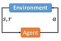
(a) MDP

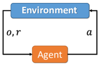
(b) POMDP

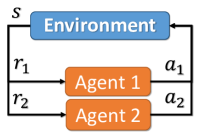
(c) Markov Game (MG)

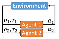
(d) POMG

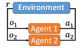
(e) Dec-POMDP

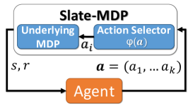
(f) Slate-MDP

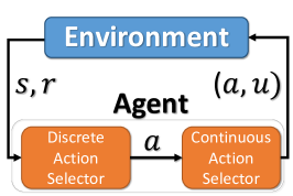
(g) Parameterized Action MDP

Figure 2: An overview of the problem formulations discussed in this survey. Within these formulations we have the following variables: states $s$, rewards $r$, actions $a$, and observations $o$. For the Parameterized Action MDP we differentiate between discrete actions $a$ and continuous actions $u$.

3.1 Markov Decision Process

Markov Decision Processes (MDPs) describe a class of problems – fully observable environments – that defines the field of RL, providing a suitable model to formulate interactions between reinforcement learners and their environment [sutton2018reinforcement]. Formally: An MDP is a tuple $\mathcal{M}=\langle\mathcal{S},\mathcal{A},\mathcal{R},\mathcal{P}\rangle$, where: $\mathcal{S}$ is a finite set of states; for each state $s\in\mathcal{S}$ there exists a finite set of possible actions $\mathcal{A}$; $\mathcal{R}$ is a real-valued payoff function $\mathcal{R}:\mathcal{S}\times\mathcal{A}\times\mathcal{S}^{\prime}\rightarrow\mathbb{R}$, where $\mathcal{R}_{a}(s,s^{\prime})$ is the expected payoff following a state transition from $s$ to $s^{\prime}$ using action $a$; $\mathcal{P}$ is a state transition probability matrix $\mathcal{P}:\mathcal{S}\times\mathcal{A}\times\mathcal{S}^{\prime}\rightarrow[0,1]$, where $\mathcal{P}_{a}(s,s^{\prime})$ is the probability of state $s$ transitioning into state $s^{\prime}$ using action $a$. MDPs can have terminal (absorbing) states at which the episode ends.

3.2 Partially Observable Markov Decision Process

Numerous environments lack the full observability property of MDPs [oliehoek2015concise]. Here, a Partially Observable MDP (POMDP) extends an MDP $\mathcal{M}$ by adding $\langle\Omega,\mathcal{O}\rangle$, where: $\Omega$ is a finite set of observations; and $\mathcal{O}$ is an observation function defined as $\mathcal{O}:\mathcal{S}\times\mathcal{A}\times\Omega\rightarrow[0,1]$, where $\mathcal{O}(o\rvert s,a)$ is a distribution over observations $o$ that may occur in state $s$ after taking action $a$.

3.3 Markov Games

Many environments, including the ones that are the focus of this survey, feature more than one learning agent. Here, game theory offers a solution via Markov games (also known as stochastic games [shapley1953stochastic]). A Markov game is defined as a tuple $(n,\mathcal{S},\mathcal{A},\mathcal{P},\mathcal{R})$, that has a finite state space $\mathcal{S}$; for each state $s\in\mathcal{S}$ a joint action space $(\mathcal{A}_{1}\times...\times\mathcal{A}_{n})$, with $\mathcal{A}_{p}$ being the number of actions available to player $p$; a state transition function $\mathcal{P}:\mathcal{S}_{t}\times\mathcal{A}_{1}\times...\times\mathcal{A}_{n}\times\mathcal{\mathcal{S}}_{t+1}\rightarrow[0,1]$, returning the probability of transitioning from a state $s_{t}$ to $s_{t+1}$ given an action profile $a_{1}\times...\times a_{n}$; and for each player $p$ a reward function: $\mathcal{\mathcal{R}}_{p}:\mathcal{\mathcal{S}}_{t}\times\mathcal{\mathcal{A}}_{1}\times...\times\mathcal{\mathcal{A}}_{n}\times\mathcal{\mathcal{S}}_{t+1}\rightarrow\mathbb{R}$ [shapley1953stochastic]. We allow terminal states at which the game ends. Each state is fully-observable.

3.4 Partially Observable Markov Games

As with POMDPs, we cannot assume the full observability property required by Markov games. A Partially Observable Markov Game (POMG) is an extension of Markov Games that includes $\langle\Omega,\mathcal{O}\rangle$ a set of joint observations $\Omega$; and an observation probability function defined as $\mathcal{O}_{p}:\mathcal{S}\times\mathcal{A}_{1}\times...\times\mathcal{A}_{n}\times\Omega\rightarrow[0,1]$. For each player $p$ the observation probability function $\mathcal{O}_{p}$ is a distribution over observations $o$ that may occur in state $s$, given an action profile $a_{1}\times...\times a_{n}$.

3.5 Decentralized-POMDPs

A Decentralized-POMDP (Dec-POMDP) is a Partially Observable Markov Game where, at each step, all $n$ agents receive an identical reward [oliehoek2015concise].

3.6 Slate Markov Decision Processes

Some environments such as recommender systems require a custom model. Here, Slate-MDPs provide a solution [sunehag2015deep]. Given an underlying MDP $\mathcal{M}=\langle\mathcal{S},\mathcal{A},\mathcal{P},\mathcal{R}\rangle$, a Slate-MDP is a tuple $\langle\mathcal{S},\mathcal{A}^{l},\mathcal{P}^{\prime},\mathcal{R}^{\prime}\rangle$. Within this formulation $\mathcal{A}^{l}$ is a finite discrete action space $\mathcal{A}^{l}=\{\bm{a}_{1},\bm{a}_{2},...,\bm{a}_{N}\}$, representing the set of all possible slates to recommend given the current state $s$. Each slate can be formulated as $\bm{a}_{i}=\{a_{i}^{1},a_{i}^{2},...a_{i}^{K}\}$, with $K$ representing the size of the slate. Slate-MDPs assume an action selection function $\varphi:\mathcal{S}\times\mathcal{A}^{l}\rightarrow\mathcal{A}$. State transitions and rewards are, as a result, determined via functions $\mathcal{P}^{\prime}:\mathcal{S}\times\mathcal{A}^{l}\times\mathcal{S}^{\prime}\rightarrow[0,1]$ and $\mathcal{R}^{\prime}:\mathcal{S}\times\mathcal{A}^{l}\times\mathcal{S}^{\prime}\rightarrow\mathbb{R}$ respectively. Therefore, given an underlying MDP $\mathcal{M}$, we have $\mathcal{P}^{\prime}(s,\bm{a},s^{\prime})=\mathcal{P}(s,\varphi(\bm{a}),s^{\prime})$ and $\mathcal{R}^{\prime}(s,\bm{a},s^{\prime})=\mathcal{R}(s,\varphi(\bm{a}),s^{\prime})$. Finally, there is an assumption that the most recently executed action can be derived from a state via a function $\psi:\mathcal{S}\rightarrow\mathcal{A}$. Note, there is no requirement that $\psi(s_{t+1})\in\bm{a}_{t}$, therefore, the action selected can also be outside the provided slate .

3.7 Parameterized Action MDPs

Parameterized Action MDPs (PA-MDPs) are a generalization of MDPs where the agent must choose from a discrete set of parameterized actions [wei2018hierarchical, masson2016reinforcement]. More formally, PA-MDPs assume a finite discrete set of actions $\mathcal{A}_{d}=\{a_{1},a_{2},...,a_{n}\}$ and for each action $a\in\mathcal{A}_{d}$ a set of continuous parameters $u_{a}\subseteq\mathbb{R}^{m_{a}}$, where $m_{a}$ represents the dimensionality of action $a$. Therefore, an action is a tuple $(a,u)$ in the joint action space, $\mathcal{A}=\bigcup_{a\in\mathcal{A}_{d}}\{(a,u)\rvert\ \mathcal{U}_{a}\}$.

3.8 Types of Action Spaces

From the above definitions we see that environments have different requirements with regard to their action spaces [9231687]. This survey will discuss approaches for:

Discrete actions $a\in\{0,1,...N\}$, with $N\in\mathcal{N}$ available actions in a given state.

MultiDiscrete action vectors $\bm{a}$. Each $a_{i}$ is a discrete action with $N$ possibilities.

Continuous actions, where an action $a\in\mathbb{R}$ is a real number, or a vector of real numbered actions.

Slate actions $\bm{a}=\{a_{1},a_{2},...,a_{n}\}$ from which one can be selected.

Parameterized Actions, mixed discrete-continuous, e.g., a tuple $(a,u)$ where $a$ is a discrete action, and $u$ is a continuous action.

3.9 Reinforcement Learning

The goal of an RL algorithm is to learn a policy $\pi$ that maps states to a probability distribution over the actions $\pi:\mathcal{S}\rightarrow P(\mathcal{A})$, so as to maximize the expected return $\mathbb{E}_{\pi}[\sum^{H-1}_{t=0}\gamma^{t}r_{t}]$. Here, $H$ is the length of the horizon, and $\gamma$ is a discount factor $\gamma\in[\texttt{0},1]$ weighting the value of future rewards. Many of the approaches discussed in this survey use the Q-learning algorithm introduced by Watkins [watkins1989learning, watkins1992q] as their foundation. Using a dynamic programming approach, the algorithm learns action-value estimates (Q-values) independent of the agent’s current policy. Q-values are estimates of the discounted sum of future rewards (the return) that can be obtained at time $t$ through selecting an action $a\in\mathcal{A}$ in a state $s_{t}$, providing the optimal policy is selected in each state that follows. Q-learning is an off-policy temporal-difference (TD) learning algorithm.

In environments with a low-dimensional state space Q-values can be maintained using a Q-table. Upon choosing an action $a$ in state $s$ according to a policy $\pi$, the Q-table is updated by bootstrapping the immediate reward $r$ received in state $s^{\prime}$ plus the discounted expected future reward from the next state, using a discount factor $\gamma\in\left(\texttt{0},1\right]$ and scalar $\alpha$ to control the learning rate: $Q_{k+1}(s,a)\leftarrow Q_{k}(s,a)+\alpha\big{(}r+\gamma\max_{s\in\mathcal{S}}\left[Q_{k}\left(s^{\prime},a\right)-Q_{k}\left(s,a\right)\right]\big{)}$. Many sequential decision problems have a high-dimensional state space. Here, Q-values can be approximated using a function approximator, for instance using a neural network. A recap of popular DRL approaches is provided in sota_drl_approaches.

3.10 Joint Policies

Our domain of interest can feature multiple agents. For each agent $p$, the strategy $\pi_{p}$ represents a mapping from the state space to a probability distribution over actions: $\pi_{p}:\mathcal{S}_{p}\rightarrow\Delta(\mathcal{A}_{p})$. Transitions within Markov games are determined by a joint policy. The notation $\bm{\pi}$ refers to a joint policy of all agents. Joint policies excluding agent $p$ are defined as $\bm{\pi}_{-p}$. The notation $\langle\pi_{p},\bm{\pi}_{-p}\rangle$ refers to a joint policy with agent $p$ following $\pi_{p}$ while the other agents follow $\bm{\pi}_{-p}$.

4 Environments

A number of benchmarking environments have emerged in recent years that grant learning agents access to an abstracted version of the ACO problem, including the CybORG environment [cage_cyborg_2022] and YAWNING TITAN (YT) [YAWNING]. In ACO-gyms, the Red agent is tasked with moving through the network graph, compromising nodes in order to progress. The end goal in most cases is to reach and impact a high-value target node. In all ACO-gyms, the task of the Blue agent is conceptually identical – to identify and counter the Red agent’s intrusion and advances using the available actions. These actions differ significantly per ACO-gym, with actions including scanning/monitoring for Red activity; isolating, making safe, and reducing vulnerability of nodes; and deploying decoy nodes.

Since the specific observations and actions are ACO-gym dependant, it can be surmised that these are not particular to the ACO problem. Any other environment which shares core features in its internal dynamics, and structure of observation and action spaces, should provide a suitable platform for developing methodologies to tackle ACO challenges before the ACO-gyms themselves are able to fully represent the problem. We have identified a total of 14 desirable criteria to assess the suitability of environments from other domains for developing and assessing techniques for tackling challenges in the ACO domain (see tab:allenvs).

Code: The availability of code can significantly speed-up research efforts. We only list codeless environments that offer unique properties, or require minimal effort to implement.

Adversarial: ACO is typically an adversarial game between a Blue and a Red agent.

General Sum & Team Games: Networks can span multiple geographic locations. Physical restraints, such as data transmission capacity and latency, can therefore necessitate a multi-agent reinforcement learning (MARL) approach.

Stochastic: ACO features stochastic factors, e.g., user activity, equipment failures and the likelihood of a Red attack succeeding. To meet this criteria stochastic state transitions are required. Random starting positions alone are insufficient.

Partially Observable: In all ACO-gyms, Blue must perform a scan/monitor action to observe Red activities. Future ACO-gyms are likely to further reduce observability, requiring more sophisticated Blue policies to detect Red agent actions.

Graph-Based: With ACO taking place on networks, ACO-gyms contain underlying dynamics unique to graph-based domains. Graph-based observation spaces are not necessarily required to fulfil this criteria. However, an environment being checked implies the presence of a graph structure.

Multi-Discrete: Given the high-dimensionality challenge present in both the observation and action spaces of ACO-gyms – which increase in size with the number of nodes – the presence of multiple discrete dimensions in the observation and action spaces is highly desirable.

Extensible Dimension: A property of graph-based dynamics is a dimension that can be expanded to geometrically increase the size of the composite space, e.g., the number of nodes in a network. Environments that meet this criteria allow methodologies to be tested for scalability to larger observation and action spaces.

Continuous Dimension: As ACO-gyms scale up, a subset of action dimensions might need to be treated as continuous, e.g., networks featuring a large number of IP addresses. Additionally, continuous attributes may be present in the observation spaces, representing node vulnerability for example [YAWNING]. Therefore, environments with mixed input and output types are desirable.

Traditionally Intractable: By identifying environments where the observation or action space is intractable, we indicate one of two properties that pose a significant, if not impossible, challenge to traditional RL methodologies:

1. The multi-discrete space causes an exponential scaling of the size of the space when flattened, such that it quickly becomes computationally intractable.

2. The observation or action space changes in size as a function of the environment; standard DRL methods require a consistent shape and size.

Environments that meet the above criteria pose a challenge to traditional DRL methodologies, and therefore necessitate novel algorithms or formulations. However, even current ACO-gyms do not meet all these criteria (see tab:allenvs). Below we provide a critical evaluation of current ACO-gyms.

Environment Properties
Categories	ACO	NBD	GD2D	DCC	RS	MG
General [head to column names, late after line=
, late after last line=

Table 1: An overview of the environments that we evaluated for this survey and their properties, with ✓and X indicating if the environment fulfills a criteria. The third symbol, $\nearrow$ indicates that the environment does not fulfil the criteria currently (due to enabling software features not being present, whether by design or due to incomplete implementations) but that the required features could be implemented with a modest amount of development effort, without the need for major extensions of environment scope. Along with ACO itself, other categories include: Gridworld Domains & 2D Games (GD2D), Discretised Continuous Control Games (DCC), Network-Based Domains (NBD), Recommender Systems (RS), and, Miscellaneous Games (MG). The latter is for unique environments which do not justify an additional category.

CybORG: The Cyber Operations Research Gym (CybORG) [cyborg_acd_2021] is a framework for implementing a range of ACO scenarios. It provides a common interface at two levels of fidelity in the form of a finite state machine and an emulator. The latter provides for each node: an operating system; hardware architecture; users, and; passwords [cage_cyborg_2022]. CybORG allows for both the training of Blue and Red agents. Therefore, in principle, it provides an ACO environment for adversarial learning. However, in practice further modifications are required in order to support the loading of a DRL opponent. This is due to environment wrappers (for reducing the size of the observation space and mapping actions) only being available to the agent that is being trained. Currently, the opponent within the environment instance receives raw unprocessed dictionary observations. Furthermore, while CybORG does allow for customizable configuration files, in practice we find that specifying a custom network is non-trivial.

Yawning Titan: The YT environment intentionally abstracts away the additional information used by CybORG’s emulator, facilitating the rapid integration and evaluation of new methods [YAWNING]. It is built to train ACO agents to defend arbitrary network topologies that can be specified using highly customisable configuration files. Each machine in the network has parameters that affect the extent to which they can be impacted by Blue and Red agent behaviour, including vulnerability scores on how easy it is for a node to be compromised. However, while YT is an easy to configure lightweight ACO environment, it currently lacks the ability to train Red agents, and does not support adversarial learning.

Network Attack Simulator (NASim): This ACO environment is a simulated computer network complete with vulnerabilities, scans and exploits designed to be used as a testing environment for AI agents and planning techniques applied to network penetration testing [schwartz2019autonomous]. NASim meets a number of our criteria, and supports scenarios that involve a large number of machines. However, [nguyen2020multiple] find that the probability of Red agent attacks succeeding in NASim are far greater than in reality. As a result the authors add additional rules to increase the task difficulty. NASim also does not support adversarial learning.

While ACO-gyms currently do not meet all the criteria that we have outlined above, it is likely that they will in the future. As the number of observation and action space dimensions grow with ACO-gyms maturing, so too will their scale; and since, in reality, the number of nodes on a computer network does not remain constant, neither shall the observation and action space sizes. Below we discuss a number of environments from several domains which could be used to develop and evaluate approaches designed to address a subset of the challenges identified. An overview of the environments that we evaluated is provided in tab:allenvs. Below we focus on four environments that meet a large number of ACO requirements.

MicroRTS [huang2021gym] is a simple Real-Time Strategy (RTS) game. It is designed to enable the training of RL agents on an environment which is similar to PySC2 [vinyals2017starcraft], the RL environment adaptation of the popular RTS game StarCraft II which possesses huge complexity. Therefore, MicroRTS is a lightweight version of PySC2, without the extensive (and expensive) computational requirements. The game features a gridworld-like observation space, where for a map of size $h\times w$, the observation space is of size $h\times w\times f$, where $f$ is a number of discrete features which may exist in any square. This observation space can be set to be partially observable. The action space is a large multi-discrete space, where each worker is commanded via a total of seven discrete actions. The number of workers will change during the game, making the core RTS action space intractable. In order to handle this, the authors of MicroRTS implemented action decomposition as part of the environment, and the action space is separated into the unit action space (of 7 discrete actions), and the player action space. While the authors discuss two formulations of this player action space, the one which is documented in code is the GridNet approach, whereby the agent predicts an action for each cell in the grid, with only the actions on cells containing player-owned units being carried out. This leads to a total action space size of $h\times w\times 7$. The challenge of varying numbers of agents is remarkably similar to the challenge of varying numbers of nodes in ACO. The MicroRTS environment, if action decomposition were to be stripped away, would be a strong candidate for handling large and variably-sized discrete action spaces.

Nocturne [nocturne2022] is a 2D driving simulator, built from the Waymo Open Dataset [Sun_2020_CVPR]. Agents learn to drive in a partially observable environment without having to handle direct sensor inputs, e.g., video from imaging cameras. Nocturne is a general-sum game. Each agent is required to both coordinate its own actions to reach its own goal and cooperate with others to avoid congestion. It is partially observable, with objects in the environment (both static and moving) causing occlusion of objects (from the egocentric perspective of the agent). However, it is not stochastic, with the state-transition probabilities being deterministic.

SUMO [SUMO2018] is a traffic simulation tool which allows for the implementation of complex, distributed traffic light control scenarios. While neither Python-based nor intended for RL, there exists a third-party interface for fulfilling these criteria [sumorl]. There are two configurations for this environment; single-agent, and multi-agent. For this review, we consider the multi-agent configuration, but treat it as a single-agent problem since, while the multi-agent scenario introduces greater complexity with multiple junctions needing to be controlled, it does not necessitate the use of multiple agents. The goal of an agent in SUMO is to control traffic signals at junctions in order to minimise the delay of vehicles passing through. The observation space is a small, but extensible (with regard to the number of junctions) continuous space, containing information about the amount of traffic in incoming lanes. For the action space, each set of lights is controlled by a single discrete variable, each corresponding to a configuration of lights. For example, at a two-way single intersection there are four possible configurations. However, each intersection type has a different number of configurations, meaning that the action space is not only multi-discrete, but also uneven. Further, as the intersections are connected by roads in the simulation, the environment will inevitably contain graph-like dynamics, i.e., the actions at, and traffic through, each intersection will affect the state at connected junctions. As such, the action space and dynamics of SUMO are applicable to ACO. However, the small observation space and lack of adversarial or partially observable properties limit this applicability.

RecSim [ie2019recsim] is a configurable framework for creating RL environments for recommender systems. In RecSim, an agent observes multiple sets of features from both a user and a document database, and makes document recommendations based on these. These sets of features are comprised of features from the user, their responses to previous recommendations, and the available documents for recommendation. These observations fulfil all desirable criteria related to observation spaces. Not only are they stochastic (due to randomness in the user’s behaviour) and partially observable (due to incompleteness in the visible user features), but they are also an extensible mix of discrete and continuous features which scale exponentially with both the number of documents and the number of features extracted from them. As such, the observation space of RecSim poses a complex challenge similar to that presented in ACO. The action space, however, is less remarkable. The agent must choose a number of documents to recommend, which is a multi-discrete space which is potentially extensible as the number of recommendations and documents increases. However, this is unlikely to be intractable unless the number of documents becomes vast. Nevertheless, this large space complements the novel and complex observation space, making this a strong candidate for experimenting with approaches for ACO challenges.

In summary, in this section, we have reviewed multiple environments and domains which hold some relevance to the challenges presented by ACO. While none of the environments reviewed meet all of our desirable criteria. Each challenge is represented in at least one domain. The most scarce of these challenges, but one which is core to ACO, is the presence of graph-based dynamics. These could only be found in network-based domains, and even there, not all environments possess them. Therefore, if the ACO solution being investigated aims to tackle graph-based dynamics, one would be limited to environments in this domain. Should graph-based dynamics not be required for development, there are several options for the other desirable criteria. StarCraft II presents a particularly complex challenge, even in cut-down versions of the game such as SMAC [samvelyan19smac, ellis2022smacv2], which meets a large number of our requirements. However, it is a computationally demanding environment. Micro-RTS [huang2021gym], an environment specifically designed to provide a less computationally demanding version of the problems presented by StarCraft II, is an attractive alternative. While the observation space is a simplified version of StarCraft II’s, the action space holds much of the same complexity, with variable numbers of agents posing an issue of intractability.

5 Coping with Vast High-Dimensional Inputs

Due to an ever growing means through which large amounts of data can be harvested, the curse of dimensionality is a prevalent problem for ML and data mining tasks. This has implications for DRL. Learning efficiency is reduced due to unnecessary features contributing noise [zebari2020comprehensive], and the state space can grow exponentially with the size of the state representation [burden2021latent]. Here, maintaining a sufficient sample spread over the state-action space becomes challenging [de2015importance].

Dimensionality reduction techniques are a natural choice for dealing with unnecessary/noisy features. Benefits include: the elimination of irrelevant data and redundant features, while preserving the variance of the dataset; improved data quality; reduced processing time and memory requirements; improved accuracy; shorter training and inference times (i.e., reduced computing costs), and; improved performance [zebari2020comprehensive]. Two popular approaches are feature selection and feature extraction. Feature selection aims to find the optimal sub-set of relevant features for training a model, which is an Non-deterministic Polynomial (NP)-hard problem [meiri2006using]. In contrast, feature extraction involves creating linear combinations of the features, while preserving the original relative distances in the latent structures. The dimensionality is decreased without losing much of the initial information [zebari2020comprehensive]. However, the resulting encodings are uninterpretable for humans.

DRL uses Deep Neural Networks (DNNs) to directly extract features from high-dimensional data [mousavi2018deep, almasan2022deep]. Nevertheless, feature selection can provide a valuable pre-processing step for training DNNs. For example, anomaly detection DNNs for cyber security applications, tasked with differentiating benign from malicious packets, were found to perform better when trained on data where feature selection had been applied [9216403].

Below we will provide an overview of DNNs used in DRL for feature extraction. Then we shall discuss state of the art DRL approaches for further eliminating unnecessary information through learning abstract states and discuss advanced exploration strategies towards enabling the sufficient visitation of all relevant states to obtain accurate utility estimates [burden2021latent, pmlr-v134-perdomo21a]. Finally, we shall take a closer look at approaches towards mitigating catastrophic forgetting, DNN’s tendency to unlearn previous knowledge [pmlr-v119-ota20a, de2015importance]. A summary of the approaches discussed in this section is provided in tab:state_abstraction in appendix:states.

5.1 Function Approximators

Many of the successes in RL over the past decade rely on the ability of DNNs to identify intricate structures and extract compact features from complex high-dimensional samples  [Goodfellow-et-al-2016, karpathy2014large, lecun2015deep]. These approaches work well for numerous domains that confront learners with the curse of dimensionality, such as the Arcade Learning Environment (ALE) [bellemare2013arcade], where DNNs are used to encode image observations. However, many of these domains are fully observable and contain state spaces with a dimensionality that is manageable for current DNNs. In contrast, this survey is focused on environments where the architectures used by standard DRL approaches cannot scale, necessitating innovative solutions. Here, considerations are required with respect to efficiently encoding an overwhelmingly large observation space to a low dimensional representation, while limiting concessions regarding performance. First, we will discuss two popular feature extraction techniques used by DRL: Convolutional Neural Networks (CNNs) and Graph Neural Networks (GNNs).

Convolutional Neural Networks: CNNs can be optimized to extract features from high dimensional arrays and tensors via multiple stacked linear convolution and pooling layers, banks of filters which are convolved with an input to produce an output map [lecun2015deep, Goodfellow-et-al-2016]. The first layer may learn to extract edges, which can then be combined into corners and contours by the subsequent layers. These features can be combined to form the object parts that enable a classification, for instance through adding fully connected layers that precede the output layer [lecun2015deep, Goodfellow-et-al-2016].

CNNs have a large learning capacity and can be trained to implement complex functions that are sensitive towards minute details within inputs  [lecun2015deep, krizhevsky2012imagenet, wu2019wider]. DNNs can be trained end-to-end using stochastic gradient descent via the back-propagation procedure, providing that the network consists of smooth functions [Goodfellow-et-al-2016]. CNNs take advantage of assumptions regarding the location of pixel dependencies within images. This allows CNNs to reduce the number of weighted connections compared to fully-connected DNNs [krizhevsky2012imagenet]. However, while CNNs are still considered a state-of-the-art (SOTA) approach for processing data in the form of arrays and tensors, there are formulations where CNNs are not directly applicable, for instance: graph-based representations.

Graph Neural Networks: Graph-based representations are a popular choice for many domains, such as traffic forecasting, drug discovery, and ACO [munikoti2022challenges]. Conventional DNNs are not applicable to graphs, due to the graph’s uneven structure, irregular size of unordered nodes, and dynamic neighbourhood compositions [kipf2016semi]. Here, GNNs have emerged as a powerful tool [JIANG2022117921]. GNNs have successfully been applied to graphs that systematically model relationships between node entities, and represent simplified versions of complex problems. Tasks include node classification, link prediction, community detection and graph classification [you2019position]. GNNs model both graph structure and node attributes via a message passing scheme, propagating relevant feature information of nodes to their neighbours until a stable equilibrium is found [kipf2016semi]. GNNs are primarily applicable to environments where graphs can be used to capture relationships between entities [munikoti2022challenges], e.g., enabling an effective factorisations of value functions for Multi-Agent Reinforcement Learning (MARL) in the StarCraft Multi-Agent Challenge (SMAC) [kortvelesy2022qgnn], or for modelling relationships between agents and objects in multi-task DRL [hong2022structureaware].

[munikoti2022challenges] recently conducted a survey on the opportunities and challenges for graph-based DRL, defining an idealised GNN for DRL as: i.) dynamic; ii.) scalable; iii.) providing generalizability, and; iv.) applicable to multiagent systems. Dynamic refers to DRL’s need for GNN approaches that can cope with time varying network configurations and parameters, e.g., the number of hosts varying over time. While GNN architectures have been proposed for dynamic graphs (e.g., spatial-temporal GNNs [nicolicioiu2019recurrent]), tasks including node classification, link prediction, community detection, and graph classification could benefit from further improvements [munikoti2022challenges]. With regard to generalizability, there is a danger that a DRL agent can overfit on the graph structure(s) seen during training, and is unable to generalize across different graphs [munikoti2022challenges].

Three popular GNNs currently receiving attention from the DRL community are [munikoti2022challenges]:

1.) Graph Convolutional Networks (GCNs): Using a semi-supervised learning approach, GCNs were the first GNNs to apply convolutional operations similar to those used by CNNs to learn from graph-structured data [kipf2016semi]. The model can learn encodings for local graph structures and the features of nodes. GCNs scale linearly in the number of graph edges. However, the entire graph adjacency matrix is required to learn these representations. Therefore, GCNs cannot generalize over graphs of different sizes [munikoti2022challenges]. This has implications for DRL, since it restricts the usage of GCNs to tasks with a static network configuration.

2.) GraphSAGE learns the topological node structure and the distribution of node features within a confined neighbourhood, computing a node’s local role in the graph along with global position [hamilton2017inductive]. Using an inductive learning approach, GraphSAGE samples node features in the local neighbourhood of each node and learns a functional mapping that aggregates the information received by each node. It is scalable to graphs of different sizes, and can be applied to different sub-graphs, thereby not requiring all the nodes to be present during training.

3.) Graph Attention Networks (GAT) use masked self-attentional layers, allowing for an implicit specification of different weights for nodes in the neighbourhood, without the need for computationally expensive matrix operations or assuming knowledge of the graph structure upfront [GAT]. The approach selectively aggregates node contributions while suppressing minor structural details.

The type of GNN selected for DRL depends on the properties of the environment. For large graphs GNN approaches are required that can be applied to sub-graphs, such as GraphSAGE [hamilton2017inductive]. Position-aware GNNs [you2019position] should be used when the position of a node provides critical information [munikoti2022challenges]. Meanwhile, for dynamic graphs an appropriate approach would be to fuse GNNs with a Recurrent Neural Network (RNN) to capture a graph’s evolution over time, allowing the network to establish spatio-temporal dependencies [munikoti2022challenges]. Indeed, even for non-graph-based environment representations we must consider the impact of partial observations $o$, or a trajectory of observations $\tau=\{o_{t-n},o_{t-n+1}...o_{t}\}$. Here RNN components are also utilized to retain relevant information [lample2017playing, li2021lstm, hochreiter1997long]. This allows the learner to encode and keep track of relevant objects, e.g., the location of other agents observed during previous time-steps [lample2017playing, kapturowski2019recurrent].

5.2 State Abstraction

The aim of state abstraction is to obtain a compressed model of an environment that retains all the useful information – enabling the efficient training and deployment of a DRL agent over an abstract formulation. Solving the abstract MDP is equivalent to solving the underlying MDP [pmlr-v108-abel20a, abel2019state, burden2018using, burden2021latent]. State abstraction groups together semantically similar states, abstracting the state space to a representation with lower dimensions [yu2018towards]. A motivating example for the importance of state abstraction is the ALE game Pong [bellemare2013arcade], where success only requires access to the positions and velocities of the two paddles and the ball [pmlr-v97-gelada19a].

[abel2019state] identify various types of abstraction discussed in the literature that can involve states and also actions, including: state abstraction [pmlr-v80-abel18a], temporal abstraction [precup2000temporal], state-action abstractions [pmlr-v108-abel20a], and hierarchical RL approaches [kulkarni2016hierarchical, dietterich2000overview]. In this section we shall focus our attention on state abstraction. Formally, given a high-dimensional state space $\mathcal{S}$, the goal of state abstraction is to implement a mapping $\phi:\mathcal{S}\rightarrow\mathcal{S}_{\phi}$ from each state $s\in\mathcal{S}$ to an abstract state $s_{\phi}\in\mathcal{S}_{\phi}$, where $\rvert\mathcal{S}_{\phi}\rvert\ll\rvert\mathcal{S}\rvert$ [abel2019theory], and $\phi$ is an encoder [abel2019theory]. This expands the set of RL problem definitions defined in sec:background, introducing the notion of an Abstract MDP, as illustrated in fig:state_abstraction.

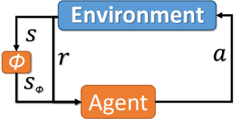
Figure 3: Depiction of an Abstract MDP, that includes a mapping $\phi:\mathcal{S}\rightarrow\mathcal{S}_{\phi}$ from the full state $s$ to an abstract state $s_{\phi}$.

In practice low dimensional representation are often obtained using Variational AutoEncoder (VAE) based architectures [kingma2013auto]. For example, [9287851] apply neural discrete representation learning, mapping high-dimensional raw video observations from an RL agent’s interactions with the environment to a low dimensional discrete latent representation, using a Vector Quantized AutoEncoder (VQ-AE) trained to reconstruct the raw video data. The benefits of the approach are demonstrated within a 3D navigation task in a maze environment constructed in Minecraft.

The work from [9287851] and others [tang2017exploration, burden2018using, burden2021latent] demonstrates the ability of state abstraction to reduce noise from raw high-dimensional inputs. However, discarding too much information can result in the encoder failing to preserve essential features. Therefore, encoders must find a balance between appropriate degree of compression and adequate representational power [abel2016near]. Using apprenticeship learning, where the availability of an expert demonstrator providing a policy $\pi_{E}$ is assumed, [abel2019state] seek to understand the role of information-theoretic compression in state abstraction for sequential decision making. The authors draw parallels between state-abstraction for RL and compression as understood in information theory. The work focuses on evaluating the extent to which an agent can perform on par with a demonstrator, while using as little (encoded) information as possible. Studying this property resulted in a novel objective function with which a VAE [kingma2013auto] can be optimized, enabling a convergent algorithm for computing latent embeddings with a trade-off between compression and value.

[pmlr-v97-gelada19a] and [zhanglearning] observe that encoder-decoder approaches are typically task agnostic – encodings represent all dynamic elements that they observe, even those which are not relevant. An idealised encoder, meanwhile, would learn a robust representation that maps two observations to the same point in the latent space while ignoring irrelevant objects that are of no consequence to our learning agent(s). Both works rely on the concept of bisimulation to avoid training a decoder. The intuition behind bisimulation is as follows.

Definition 5.1 (Bisimulation.).

Given an MDP $\mathcal{M}$, an equivalence relation $B$ between states is a bisimulation relation if, for all states $s_{i},s_{j}\in\mathcal{S}$ that are equivalent under B (denoted $s_{i}\equiv_{B}s_{j}$ ) the following conditions hold:

$$\mathcal{R}(s_{i},a)=\mathcal{R}(s_{j},a),\forall a\in\mathcal{A},$$ (1)

$$\mathcal{P}(G\rvert s_{i},a)=\mathcal{P}(G\rvert s_{j},a),\forall a\in\mathcal{A},\forall G\in\mathcal{S}_{B},$$ (2)

where $\mathcal{S}_{B}$ is the partition of $\mathcal{S}$ under the relation $B$ (the set of all groups $G$ of equivalent states), and $\mathcal{P}(G\rvert s,a)=\sum_{s^{\prime}\in G}\mathcal{P}(s^{\prime}\rvert s,a)$.

[zhanglearning] propose deep bisimulation for control (DBC) that learns directly on a bisimulation distance metric. This allows the learning of invariant representations that can be used effectively for downstream control policies, and are invariant with respect to task-irrelevant details. The encoders are trained in a manner such that distances in latent space equal bisimulation distances in the actual state space. The authors evaluated their approach on visual Multi-Joint dynamics with Contact (MuJoCo) tasks where control policies must be learnt from natural videos with moving distractors in the background. Exactly partitioning states with bisimulation is generally not feasible when dealing with a continuous state space, therefore a pseudometric space $(\mathcal{S},d)$ is utilized, where distance function $d:\mathcal{S}\times\mathcal{S}\rightarrow\mathbb{R}_{\geq 0}$ measures the similarity between two states. DBC significantly outperforms SAC and DeepMDP [gelada2019deepmdp] on CARLA, an open-source simulator for autonomous driving research . While DBC was applied to image data, in principle it could also be applied to observations from ACO domains.

5.3 Exploration

Successful state abstraction has numerous applications, including the scaling of principled exploration strategies to DRL [tang2017exploration] and potential-based reward shaping [burden2021latent, burden2018using]. However, learning an abstract state space that meets all the desired criteria remains a long-standing problem. RL agents often gradually unlock new abilities, that in turn result in new areas of the environment being visited. Many initial encodings may be learned before an agent has sufficiently explored the state space [pmlr-v119-misra20a]. In addition, exploration is intractable for domains suffering from the curse of dimensionality. Principled exploration strategies are required that enable the sufficient visitation of abstracted states  [burden2021latent, pmlr-v119-misra20a, wong2022deep]. To address this, [pmlr-v119-misra20a] introduce HOMER, a state abstraction approach that accounts for the fact that the learning of a compact representation for states requires comprehensive information from the environment - something that cannot be achieved via random exploration alone.

HOMER is designed to learn a reward-free state abstraction termed kinematic inseparability, aggregating observations that share the same forward and backward dynamics. The approach iteratively explores the environment by training policies to visit each kinematically inseparable abstract state. Policies are constructed using contextual bandits and a synthetic reward function that incentifies agents to reach an abstract state. In addition, HOMER interleaves learning the state abstraction and the policies for reaching the new abstract states in an inductive manner, meaning policies reach new states, which are abstracted, and then new policies are learned, iteratively, until a policy cover has been obtained. This iterative learning approach is depicted in fig:homer. Once HOMER is trained a near-optimal policy can be found for any reward function. HOMER outperforms PPO and other baselines on an environment named the diabolical combination lock, a class of rich observation MDPs where the wrong choice leads to states from which an optimal return is impossible.

Figure 4: HOMER (Adapted from [pmlr-v119-misra20a]).

There are numerous count-based exploration approaches with strong convergence guarantees for tabular RL when applied to small discrete Markov decision processes [tang2017exploration]. [ladosz2022exploration] define three desirable criteria for exploration methods, including: i.) determining the degree of exploration based on the agent’s learning; ii.) encouraging actions that are likely to result in new outcomes, and; iii.) rewarding the agent for exploring environments with sparse rewards. A popular approach towards encouraging exploration is via intrinsic rewards, where the reward signal consists of extrinsic and intrinsic components. When combined with state-abstraction, these tried and tested methods can be applied to environments suffering from the curse of dimensionality.

[tang2017exploration] introduce a count-based exploration method through static hashing, using SimHash. The hash codes are obtained via a trained AutoEncoder, and provide a means through which to keep track of the number of times semantically similar observation-action pairs have been encountered. A count-based reward encourages the visitation of less frequently explored semantically similar observation-action pairs. [bellemare2016unifying] proposed using Pseudo-Counts, counting salient events derived from the log-probability improvement according to a sequential density model over the state space. In the limit this converges to the empirical count. [martin2017count] focus on counts within the feature representation space rather than for the raw inputs. Other approaches for computing intrinsic rewards are based on prediction errors  [pathak2017curiosity, stadie2015incentivizing, savinovepisodic, burdaexploration, bougie2021fast, ladosz2022exploration] and memory based methods [fu2017ex2, badianever], using models trained to distinguish states from one another, where easy to distinguish states are considered novel [ladosz2022exploration].

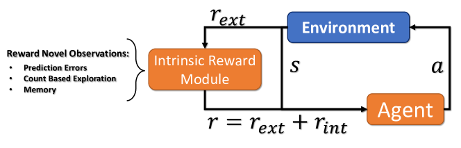
Figure 5: Approaches rewarding agents for visiting novel states (Adapted from [ladosz2022exploration]).

Goal based exploration represents another class of methods, which [ladosz2022exploration] further divide into: meta-controllers, where a controller with a high-level overview of the environment provides goals for a worker agent [forestier2017intrinsically, colas2019curious, vezhnevets2017feudal, hester2013learning, kulkarni2016hierarchical]; sub-goals, finding a sub-goal for agents to reach, e.g., bottlenecks in the environment [machado2017laplacian, machadoeigenoption, fangadaptive], and; goals in the region of highest uncertainty, where exploring uncertain states with respect to the rewards are the sub-goals [kovac2020grimgep].

Despite the above advances, learning over the entirety of the environment is neither feasible nor desirable when dealing with increased complexity. Here principled methods are required that can determine which parts of the state space are most relevant [pmlr-v134-perdomo21a]. However, this requirement in itself leads to the dilemma of how one can determine with minimal effort that an area of the state space is irrelevant, which is an open research question.

5.4 Knowledge Retention

As with many online learning tasks, DRL agents are prone to catastrophic forgetting: the unlearning of previously acquired knowledge [atkinson2021pseudo, schak2019study]. In order to be sample efficient, DRL approaches often resort to experience replay memories, which store experience transition tuples that are sampled during training [foerster2017stabilising]. Samples are either stored long term, as in off-policy approaches such as DQN and DDPG, or short term, e.g., samples gathered using multiple workers for PPO. For the former, paying attention to the experience replay memory composition can mitigate catastrophic forgetting [de2015importance]. However, in practice, a large number of transitions are discarded, since there is a memory cost associated with storage.

An additional challenge is that the stationarity of the environment, and one’s opponent(s), are a strong assumption. Samples stored inside a replay buffer can become deprecated, confronting learners with the same challenges seen in data streaming [hernandez2018multiagent]. Here DRL agents require continual learning, the ability to continuously learn and build on previously acquired knowledge [wolczyk2021continual].

One approach to solve this problem is to utilize a dual memory where a freshly initialized DRL agent, a short-term agent (network), is trained on a new task, upon which knowledge is transferred to a DQN designed to retain long-term knowledge from previous tasks. A generative network is used to generate short sequences from previous tasks for the DQN to train on, in order to prevent catastrophic forgetting as the new task is learned [atkinson2021pseudo]. However, this approach relies on a stationary environment, as an additional mechanism would be required to determine the relevance of past knowledge, given drift in the state transition probabilities.

Elastic Weight Consolidation (EWC) is another popular approach for mitigating catastrophic forgetting for DNNs [kirkpatrick2017overcoming, huszar2018note, huszar2017quadratic]. EWC has been applied to DRL using an additional loss term using the Fisher information matrix for the difference between the old and new parameters, and a hyperparameter $\lambda$ which can be used to specify how important older weights are [ribeiro2019multi, nguyen2017system, kessler2022same, wolczyk2021continual].

6 Approaches for combinatorial action spaces

Due to an explosion in the number of state-action pairs, traditional DRL approaches do not scale to high-dimensional combinatorial action spaces. Scalable methods will need to meet the following criteria.

Generalizability: For our target domains a sufficient visitation of all state-action pairs to obtain accurate value estimates is intractable. Formulations are required that allow for generalization over the action space [dulac2015deep].

Time-Varying Actions (TVA) can result in a policy being trained on a subset of actions $\mathcal{A}^{\prime}\subset\mathcal{A}$. This has implications when the agent is later asked to choose from a larger set of actions [9507301] or applying actions to previously unseen objects [chandak2020lifelong, fang2020learning, 9507301], e.g., a new host on a network for ACO.

Computational Complexity: An efficient formulation is to use a DNN with $\rvert\mathcal{A}\rvert$ output nodes, requiring a single forward pass to compute an output for each action. However, this approach will not generalize well. Alternatively, for a value function with a single output, one could input observation-action pairs and estimate the utility of an arbitrary number of actions: $Q:\mathcal{O}\times\mathcal{A}\rightarrow\mathbb{R}$. However, this approach is intractable due to the computational cost growing linearly with $\rvert\mathcal{A}\rvert$. Instead, methods with sub-linear complexity are required.

The criteria listed above provide the axes along which the suitability of approaches for our target domains can be measured. Through reviewing the literature on high-dimensional action spaces we were able to identify five categories that conveniently cluster the approaches: i.) proto action based approaches; ii.) action decomposition; iii.) action elimination; iv.) hierarchical approaches, and; v.) curriculum learning. fig:high_level_action_approaches_categories provides an illustrative example and short description for each category. In tab:high_dim_action_approaches in appendix:action_approaches we provide an overview of the literature and a short contributions summary.

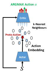
(a) Proto Actions

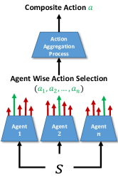
(b) Action Decomp.

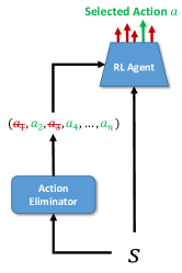
(c) Action Elimination

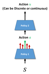
(d) Hierarchical

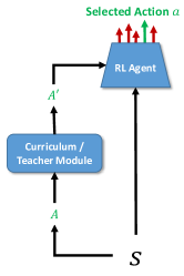
(e) Curriculum

Figure 6: Categories of DRL approaches for high-dimensional action spaces. fig:actions:proto: Proto actions leverage prior domain knowledge and embed actions into a continuous space, before applying $k$-NN to pick the closest discrete actions, which are passed to a critic. fig:actions:composition: Action Decomposition reformulates the single agent problem as a Dec-POMDP with a composite action space. fig:actions:elimination: Action elimination approaches use a module that determines which actions are redundant for a given observation. fig:actions:hierarchcial: Hierarchical, the action selected by a policy influences the action selected by a sub-policy. fig:actions:curriculum: Curriculum learning approaches for gradually increasing the number of available actions.

6.1 Proto Action Approaches

[dulac2015deep] proposed the first DRL approach to address the high dimensional action space problem, the Wolpertinger architecture, which embeds discrete actions into a continuous space $\mathbb{R}^{n}$. A continuous control policy $f_{\pi}:\mathcal{O}\rightarrow\mathbb{R}^{n}$, is trained to output a proto action. Given that a proto action $\hat{a}$ is unlikely to be a valid action ($\hat{a}\notin\mathcal{A}$), $k$-nearest-neighbours ($k$-NN) is used to map the proto action to the $k$ closest valid actions: $g_{k}(\hat{a})=\operatorname*{argmin}_{a\in\mathcal{A}}^{k}\rvert a-\hat{a}\rvert_{2}$. To avoid picking outlier actions, and to refine the action selection, the selected actions are passed to a critic $Q$, which then selects the $\operatorname*{argmax}$ (see Algorithm alg:WolpertingerPolicy).

Algorithm 1 Wolpertinger Policy [dulac2015deep]

1:Receive an observation $o$ from the environment.

2:$\hat{a}=f_{\pi}(o)$ $\triangleright$ Obtain proto-action from the actor.

3:$\mathcal{A}_{k}=g_{k}(\hat{a})$ $\triangleright$ Get $k$ nearest neighbours.

4:$a=\operatorname*{argmax}_{a_{j}\in\mathcal{A}_{k}}Q(o,a_{j})$ $\triangleright$ Action refinement step.

5:Apply $a$ to environment and receive $r$, $o^{\prime}$.

The Wolpertinger architecture meets many of the above requirements. While the time-complexity scales linearly with the number of actions $k$, the authors show both theoretically and in practice that there is a point at which increasing $k$ delivers a marginal performance increase at best. Using 5-10% of the maximal number of actions was found to be sufficient, allowing agents to generalize over the set of actions with sub-linear complexity. Here, the action embedding space does require a logical ordering of the actions along each axis. Currently prior information about the action space is leveraged to construct the embedding space. However, [dulac2015deep] note that learning action representations during training could also provide a solution. The approach has also been criticised for instability during training due to the $k$-NN component preventing the gradients from propagating back to boost the training of the actor network [tran2022cascaded].

Wolpertinger has been applied to: caching on edge devices to reduce data traffic in next generation wireless networks  [zhong2018deep], voltage control for shunt compensations to enhance voltage stability [cao2020optimal], maintenance and rehabilitation optimization for multi-lane highway asphalt pavement [9750983], recommender systems (Slate-MDPs) [sunehag2015deep, 10.1145/3240323.3240374, DBLP:journals/corr/abs-1801-00209], and, penetration testing for ACO [nguyen2020multiple]. For the latter, [nguyen2020multiple] evaluate the ability of Wolpertinger to learn a policy that launches attacks on vulnerable services on a network. Wolpertinger is applied using an embedding space that consists of three levels (illustrated in fig:NASim_attack_embedding): i.) the action characteristics (scan subnet, scan host and exploit services); ii.) the subnet to target, and; iii.) services that are vulnerable towards attacks. The second dimension focuses on the destination of the action with respect to the subnet, e.g., selecting scan subnet along axis $1$ and selecting the subnet on axis $2$. Node2Vec is used for expressing the network structure, and the authors also train a network to produce similar embeddings for correlated service vulnerabilities. Wolpertinger was shown to outperform DQN on the Network Attack Simulator environment [schwartz2019autonomous].

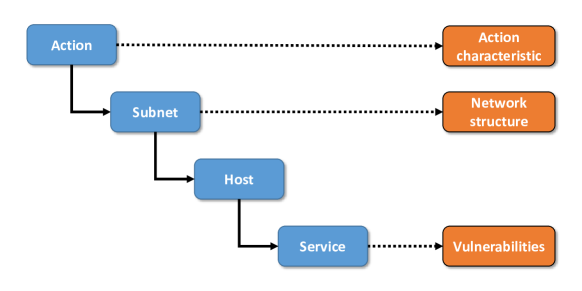
Figure 7: Wolpertinger attack embedding used by [nguyen2020multiple] on NASim [schwartz2019autonomous].

6.2 Action Decomposition Approaches

A popular approach towards scaling DRL to large combinatorial action spaces is to apply multi-agent deep reinforcement learning (MADRL). The action space is decomposed into actions provided by multiple agents, e.g., having each agent control an action dimension [tavakoli2018action], or via an algebraic formulation for combining the actions [tran2022cascaded]. However, learning an optimal policy requires the underlying agents to converge upon an optimal joint-policy. Therefore, approaches must be viewed through the lens of MADRL within a Dec-POMDP, using equilibrium concepts from multi-agent learning.

Formally, given an expected gain, ${\mathcal{G}}_{i}(\bm{\pi})=\mathbb{E}_{\bm{\pi}}\{\sum_{k=0}^{\infty}\gamma^{k}r_{i,t+k+1}\rvert x_{t}=x\}$, the underlying policies must find a Pareto optimal solution, i.e., a joint policy $\bm{\hat{\pi}}$ from which no agent $i$ can deviate without making at least one other agent worse off [matignon2012independent]:

Definition 6.1 (Pareto Optimality).

A joint-strategy $\bm{\pi}$ is Pareto-dominated by $\bm{\hat{\pi}}$ if and only if (iff):

$$\forall i,\forall s\in\mathcal{S},\mathcal{G}_{i,\bm{\hat{\pi}}}(s)\geq\mathcal{G}_{i,\bm{\pi}}(s)\ and\ \exists j,\exists s\in\mathcal{S},\mathcal{G}_{j,\bm{\hat{\pi}}}(s)>\mathcal{G}_{j,\bm{\pi}}(s).$$ (3)

A joint policy $\bm{\hat{\pi}}^{*}$ is Pareto optimal if it is not Pareto-dominated by any other $\bm{\pi}$.

There are three categories of training schemes for cooperative MA(D)RL (illustrated in fig:marl_approaches_overview): independent learners (ILs), who treat each other as part of the environment; the centralized controller approach, which does not scale with the number of agents; and centralized training for decentralized execution (CTDE).

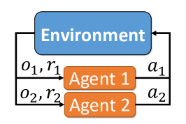
(a) Independent Learners

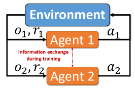
(b) Centralized Training for Decenctralized Execution

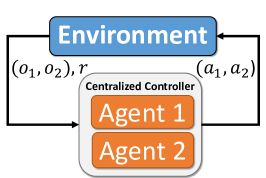
(c) Centralized Controller

Figure 8: An overview of multi-agent reinforcement learning training schemes.

Even within stateless two player matrix games with a small number of actions per agents, ILs fail to consistently converge upon Pareto optimal solutions [nowe2012game, claus1998dynamics, matignon2012independent, kapetanakis2002reinforcement, matignon2007hysteretic, busoniu2008comprehensive, panait2006lenient, panait2008theoretical]. However, ILs are frequently used as a baseline for action decomposition approaches [tavakoli2018action]. Therefore, to better understand the challenges that confront action decomposition approaches we shall first briefly consider the multi-agent learning pathologies that learners must overcome to converge upon a Pareto optimal joint-policy from the perspective of ILs :

Miscoordination occurs when there are two or more incompatible Pareto-optimal equilibria [claus1998dynamics, kapetanakis2002reinforcement, matignon2012independent]. One agent choosing an action from an incompatible equilibria is sufficient to lower the gain. Formally: two equilibria $\bm{\pi}$ and $\bm{\hat{\pi}}$ are incompatible iff the gain received for pairing at least one agent using a policy $\pi$ with other agents using a policy $\hat{\pi}$ results in a lower gain compared to when all agents are using $\pi$: $\exists i,\bm{\pi}_{i}\neq\bm{\hat{\pi}}_{i},\mathcal{G}_{i,\langle\bm{\hat{\pi}}_{i},\bm{\pi}_{-i}\rangle}<\mathcal{G}_{i,\bm{\pi}}$.

Relative Overgeneralization: ILs are prone to being drawn to sub-optimal but wide peaks in the reward space, as there is a greater likelihood of achieving collaboration there [panait2006lenience]. Within these areas a sub-optimal policy yields a higher payoff on average when each selected action is paired with an arbitrary action chosen by the other agent [panait2006lenience, wiegand2003analysis, palmer2020independent].

Stochasticity of Rewards and Transitions: Rewards and transitions can be stochastic, which has implications for approaches that use optimistic learning to overcome the relative overgeneralization pathology  [palmer2020independent, palmer2018negative, palmer2018lenient].

The Alter-Exploration Problem: In MA(D)RL increasing the number of agents also increases global exploration, the probability of at least one of $n$ agents exploring: $1-(1-\epsilon)^{n}$. Here, each agent explores according to a probability $\epsilon$ [matignon2012independent].

The Moving Target Problem is a result of agents updating their policies in parallel [bowling2002multiagent, sutton1998introduction, tuyls2012multiagent, tuyls2007evolutionary]. This pathology is amplified when using experience replay memories $\mathcal{D}_{i}$, due to transitions becoming deprecated [foerster2017stabilising, omidshafiei2017deep, palmer2018lenient].

Deception: Deception occurs when utility values are calculated using rewards backed up from follow-on states from which pathologies such as miscoordination and relative overgeneralization can also be back-propagated [JMLR:v17:15-417]. States with high local rewards can also represent a problem, drawing ILs away from optimal state-transition trajectories [JMLR:v17:15-417].

Non-trivial approaches are required in order to consistently converge upon a Pareto optimal solution [JMLR:v17:15-417, lauer2000algorithm, kapetanakis2002reinforcement, palmer2020independent]. We shall now consider the different types of action decomposition approaches that can be found in the literature.

6.2.1 Branching Dueling Q-Network

Designed for environments where the action-space can be split into smaller action-spaces Branching Dueling Q-Network (BDQ) [tavakoli2018action] is a branching version of Dueling DDQN [wang2016dueling] . Each branch of the network is responsible for proposing a discrete action for an actuated joint. The approach features a shared decision module, allowing the agents to learn a common latent representation that is subsequently fed into each of the $n$ DNN branches, and can therefore be considered a CTDE approach. A conceptional illustration of the approach can be found in fig:BDQ.

BDQ has a linear increase of network outputs with regard to number of degrees of freedom, thereby allowing a level of independence for each individual action dimension. It does not suffer from the combinatorial growth of standard vanilla discrete action algorithms. However, the approach is designed for discretized continuous control domains. Therefore, BDQ’s scalability to the MultiDiscrete action spaces from ACO requires further investigation.

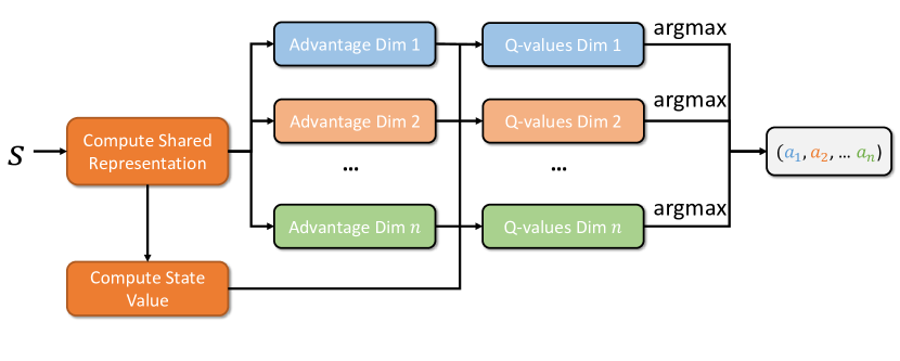
Figure 9: An illustration Branching Dueling Q-Networks (adapted from [tavakoli2018action]).

While BDQ achieves sub-linear complexity, the formulation is vulnerable towards the MA(D)RL pathologies outlined above. To evaluate the benefit of the shared decision module, BDQ is evaluated against Dueling-DQN, DDPG, and independent Dueling DDQNs (IDQ). The only mentioned distinction between BDQ and IDQ is that the first two layers were not shared among IDQ agents [tavakoli2018action]. BDQ uses a modified Prioritized Experience Replay memory [schaul2015prioritized], where transitions are prioritized based on the aggregated distributed TD error. In essence, a prioritized version of Concurrent Experience Replay Trajectories (CERTS) are being utilized, a method from the MADRL literature that has previously been shown to facilitate coordination [omidshafiei2017deep].

BDQ has been evaluated on numerous discretized MuJoCo domains [tavakoli2018action]. The evaluation focused on two axes: granularity and degrees of freedom. BDQ’s benefits over Dueling-DQNs become noticeable as the number of degrees of freedom are increased. In addition, BDQ was able to solve granular, high degree of freedom domains for which Dueling-DDQNs was not applicable. On the majority of the domains DDPG still outperformed BDQ, with the exception of Humanoid-v1. Unfortunately a comparison of BDQ against the Wolpertinger architecture was not provided. For ACO we note that BDQ will probably not scale well if one of the branches is very large, e.g., has lot of nodes.

6.2.2 Cascading Reinforcement Learning Agents

For cascading reinforcement learning agents (CRLA) the action space $\mathcal{A}$ is decomposed into smaller sets of actions $\ \mathcal{U}^{1},\ \mathcal{U}^{2},...,\ \mathcal{U}^{L}$ [tran2022cascaded]. For each subset of actions $\mathcal{A}^{i}$, the size of the dimensionality is significantly smaller than that of $\mathcal{A}$, i.e., $\rvert\ \mathcal{U}^{i}\rvert\ll\ \rvert\mathcal{A}\rvert$ $(\forall i\in[1,L])$. In this formulation a primitive action $a_{t}$ at time step $t$ is given by a function over actions $u_{t}^{i}$ obtained from each respective subset $\ \mathcal{U}^{i}$: $u_{t}=f(u_{t}^{1},u_{t}^{2},...,u_{t}^{L})$. The action components $u_{t}^{i}$ are chained together to algebraically build an integer identifier. This provides a formulation through which larger identifiers can be obtained using the smaller integer values provided by each action subset. A CTDE approach is used to facilitate the training of $n$ agents, where the joint action space $\bm{\mathcal{A}}$ is comprised of $\ \mathcal{U}^{1},\ \mathcal{U}^{2},...,\ \mathcal{U}^{n}$, with $\ \mathcal{U}^{i}$ representing the action space of an agent $i$. The concept is illustrated in fig:cascading.

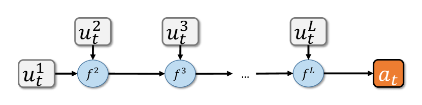
Figure 10: Action space composition. Action $u_{t}$ at time step $t$ is algebraically constructed using actions $a^{i}_{t}$ obtained from action subsets $\mathcal{A}^{i}$ (adapted from  [tran2022cascaded]).

CRLA yields a solution that allows for large combinatorial action spaces to be decomposed into a branching tree structure. Each node in the tree represents a decision by an agent regarding which child node to select next. Each node has its own identifier, and all nodes in the tree have the same branching factor, with a heuristic being used to determine the number of tree levels: $\rvert T\rvert=\log_{b}(\rvert\mathcal{A}\rvert)$. Instead of having an agent for each node, the authors propose to have a linear algebraic function that shifts the action component identifier values into their appropriate range: $u^{i+1}_{out}=f(u^{i}_{out})=u^{i}_{out}\times\beta^{i+1}+u^{i+1}$, with $\beta^{i+1}$ being the number of nodes at level $i+1$. More generally, given two actions $u^{i}$ and $u^{i+1}$ obtained from agents at levels $i$ and $i+1$, where for both actions we have identifiers in the range $[0,...,\rvert\ \mathcal{U}^{i}\rvert-1]$, and $[0,...,\rvert\ \mathcal{U}^{i+1}\rvert-1]$ respectively, then the action component identifier at level $i+1$ is $u^{i}\times\rvert\ \mathcal{U}^{i+1}\rvert+u^{i+1}$. The executive primitive action meanwhile will be computed via: $a=u^{L-1}\times\rvert\ \mathcal{U}^{L}\rvert+u^{L}$. An illustration of this tree structure is provided in fig:cascading_selection_tree.

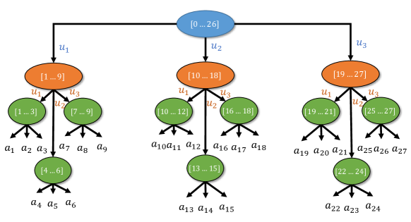
Figure 11: An illustration of the action selection process used by CRLA (adapted from [tran2022cascaded]). The leaf nodes represent the primitive actions from $\mathcal{A}$, while each internal node contains the action range for its children. Through using an algebraic formulation that makes use of an offset, only three agents with an action space $\rvert\ \mathcal{U}^{i}\rvert=3$ are needed to capture $\mathcal{A}$.

Cooperation among agents is facilitated via QMIX [rashid2018qmix], which uses a non-linear combination of the value estimates to compute the joint-action-value during training. The weights of the mixing network are produced using a hypernetwork [ha2016hypernetworks], conditioned on the state of the environment. In CRLA agents share a replay buffer. Therefore, as with BDQ, a synchronised sampling equivalent to CERTS [omidshafiei2017deep] is being used. The authors [tran2022cascaded] recommend limiting the size of the action sets to 10 – 15 actions, and to choose an $L$ that allows the approach to reconstruct the intended action set $\ \mathcal{U}$. CRLA-QMIX was evaluated on two environments against a version of CRLA using independent learners, and a single DDQN:

• A toy-maze scenario with a discretized action space, representing the directions in which the agent can move. The agent received a small negative reward for each step, and positive one upon completing the maze. An action size of 4096 was selected, with $n=12$ actuators.

• A partially observable CybORG capture the flag scenario from Red’s perspective. Upon finding a flag a large positive reward was received. A smaller reward was obtained for successfully hacking a host.

CRLA significantly outperformed DDQN on both the maze task and CybORG scenarios with more than 50 hosts. CRLA-QMIX had less variance and better stability than CRLA with ILs. However, in an evaluation scenario with 60 hosts the converged policies show similar rewards and steps per episode, potentially explained by the fact that CRLA-ILs also makes use of CERTs. The authors note that hyperparameter tuning for the QMIX hypernetwork was time consuming.

6.2.3 Discrete Sequential Prediction of Continuous Actions

[metz2017discrete] propose a Sequential DQN (SDQN) for discretized continuous control. The original (upper) MDP with $N$ (actuators) times $D$ (dimensions) actions is transformed into a lower MDP with $1\times D$ actions. The lower MDP consists of the compositional action component, where $N$ actions are selected sequentially. Unlike BDQ actuators take turns selecting actions, and can observe the actions that have been selected by others (see fig:SDQN). Also, the action composition was obtained using a single DNN that learns to generalize across actuators. An LSTM [hochreiter1997long] was used to keep track of the selected actions. For stability, SDQN learns Q-values for both the upper and lower MDPs at the same time, performing a Bellman backup from the lower to the upper MDP for transitions where the Q-value should be equal. In addition, a zero discount is used for all steps except where the state of the upper MDP changes. Another requirement is the pre-specified ordering of actions. The authors hypothesise that this may negatively impact training on problems with a large number of actuators.

The authors evaluate SDQN against DDPG on a number of continuous control tasks from the OpenAI gym [1606.01540], including Hopper ($N=3$), Swimmer ($N=2$), Half-Cheetah ($N=6$), Walker2d ($N=6$), and Humanoid($N=17$). SDQN outperformed DDPG on all domains except Walker2d. With respect to granularity SDQN required $D\geq 4$. The authors also evaluated 8 different action orderings at 3 points during training on Half Cheetah. All orderings achieved a similar performance.

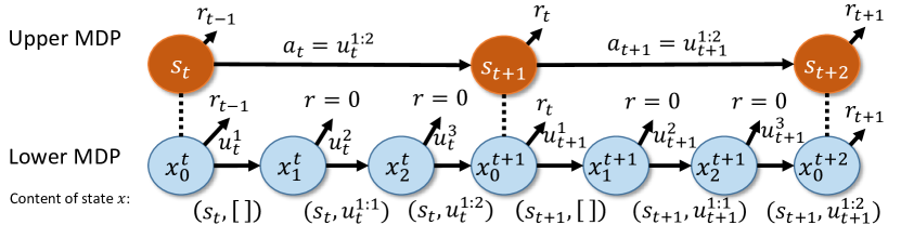
Figure 12: Sequential DQN Architecture (adapted from [metz2017discrete]).

6.2.4 Time-Varying Composite Action Spaces

[9507301] propose the Structured Cooperation Reinforcement Learning (SCORE) algorithm that accounts for dynamic time-varying action spaces, i.e., environments where a sub-set of actions become temporarily invalid [9507301]. SCORE can be applied to heterogeneous action spaces that contain continuous and discrete values. A series of DNNs model the composite action space. A centralized critic and decentralized actor (CCDA) approach [li2020f2a2] facilitates cooperation among the agents. In addition a Hierarchical Variational Autoencoder (HVAE) [edwards2017towards] maps the sub-action spaces of each agent to a common latent space. This is then fed to the critic, allowing the critic to model correlations between sub-actions, enabling the explicit modelling of dependencies between the agents’ action spaces. A graph attention network (GAT) [GAT] is used as the critic, in order to handle the varying numbers of agents (nodes). The HVAE and GAT are critical for SCORE to cope with varying numbers of heterogeneous actors. As a result, SCORE is a two stage framework, that must first learn an action space representation, before learning a robust and transferable policy. For the first phase a sufficient number of trajectories must be gathered for each sub-action space. The authors use a random policy to generate these transitions. Once the common latent action representation is acquired the training can switch to focusing on obtaining robust policies.

SCORE is evaluated on a proof-of-concept task – a Spider environment based on the MuJoCo Ant environment – and a Precision Agriculture Task, where the benefits of a mixed discrete-continuous action space comes into play. SCORE outperforms numerous baselines on both environments, including MADDPG [lowe2017multi], PPO [schulman2017proximal], SAC [haarnoja2018soft], H-PPO [fan2019hybrid], QMIX [rashid2018qmix] and MAAC [iqbal2019actor]. However, the code for the environments and SCORE are not made publicly available.

6.2.5 Action Decomposition Approaches for Slate-MDPs

Action decomposition approaches have also been applied to Slate-MDPs. Two noteworthy efforts are Cascading Q-Networks and Slate Decomposition.

Cascading Q-Networks (CDQNs): [pmlr-v97-chen19f] introduce a model-based RL approach for the recommender problem that utilizes Generative Adversarial Networks (GANs)[goodfellow2014generative] to imitate the user’s behaviour dynamics and reward function. The motivation for using GANs is to address the issue that a user’s interests can evolve over time, and the fact that the recommender system can have a significant impact on this evolution process. In contrast, most other works in this area use a manually designed reward function. A CDQN is used to address the large action space, through which a combinatorial recommendation policy is obtained. CDQNs consist of $k$ related Q-functions, where actions are passed on in a cascading fashion.

CDQNs were evaluated on six real-world recommendation datasets – MovieLens, LastFM, Yelp, Taobao, YooChoose, and Ant Financial – against a range of non-RL recommender approaches, including IKNN, S-RNN, SCKNNC, XGBOOST, DFM, W&D-LR, W&D-CCF, and a Vanilla DQN. On the majority of these datasets, the generative adversarial model is a better fit to user behaviour with respect to held-out likelihood and click prediction. With respect to the resulting model policies, better cumulative and long-term rewards were obtained. The approach took less time to adjust compared to approaches that did not make use of the GANs synthesized user. However, we caution that applying model-based RL approaches to complex asymmetrical adversarial games, such as ACO, requires further considerations.

Slate Decomposition: Slate decomposition, or SlateQ, is an approach where the Q-value estimate for a slate $\bm{a}$ can be decomposed into the item-wise Q-values of its constituent items $u_{i}$ [ie2019reinforcement]. Having a decomposition approach that can learn $\bar{Q}(s,a_{i})$ for an item $i$ mitigates the generalization and exploration challenges listed above. However, the ability to successfully factor the Q-value of a slate $\bm{a}$ relies on two assumptions: Single Choice (SC) and Reward/Transition Dependence on Selection (RTDS). The authors show theoretically that given the standard assumptions with respect to learning and exploration [sutton2018reinforcement], as well as SC and RTDS, SlateQ will converge to the true slate Q-function $Q_{\pi}(x,\bm{a})$. SlateQ is evaluated in a simulation, while validity and scalability were tested in live experiments on YouTube.

6.3 Action Elimination Approaches

Learning with a large combinatorial action space is often challenging due to a large number of actions being either redundant or irrelevant within a given state [zahavy2018learn]. RL agents lack the ability to determine a sub-set of relevant actions. However, there have been efforts towards the state dependent elimination of actions. [zahavy2018learn] combine a DQN with an action-elimination network (AEN), which is trained via an elimination signal $e$, resulting in AE-DQN (fig:aedqn). After executing an action $a_{t}$, the environment will return a binary action elimination signal in $e(s_{t},a_{t})$ in addition to the new state and reward signal. The elimination signal $e$ is determined using domain-specific knowledge. A linear contextual bandit model is applied to the outputs of the AEN, that is tasked with eliminating irrelevant actions with a high probability, balancing out exploration/exploitation. Concurrent learning introduces the challenge that the learning process of both the DQN and AEN affect the state-action distribution of the other. However, the authors provide theoretical guarantees on the convergence of the approach using linear contextual bandits. While the AE-DQN was designed for text based games the authors note that the approach is applicable to any environment where an elimination signal can be obtained via a rule-based system.

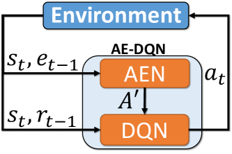
Figure 13: Action Elimination DQN (adapted from [zahavy2018learn]). The agent selects an action $a_{t}$, and observes a reward $r_{t-1}$, the next observation $o_{t}$ and an elimination signal $e_{t-1}$. The agent uses this information to learn two function approximation deep networks: a DQN and an AEN. The AEN provides an admissible actions set $\mathcal{A}^{\prime}\subseteq\mathcal{A}$ to the DQN, from which the DQN can pick the next action $a_{t+1}$.

AE-DQN is evaluated on both Zork and a $K$-Room Gridworld environment. For the $K$-rooms Gridworld environment a significant gain for the use of action elimination was observed as the number of categories $K$ was increased. Similar benefits were observed in the Zork environment, e.g., AE-DQN using 215 actions being able to match the performance of a DQN trained with a reduced action space of 35 actions, while significantly outperforming a DQN with 215 actions. However, questions remain regarding the extent to which the approach is applicable to very high dimensional action spaces, where additional considerations may be required as to how the AEN can generalize over actions.

Action elimination has also been applied to Slate-MDPs. [10.1145/3289600.3290999] adapted the REINFORCE algorithm into a top-$k$ neural candidate generator for large action spaces. The approach relies on data obtained through previous recommendation policies (behaviour policies $\beta$), which are utilized as a means to correct data biases via an importance sampling weight while training a new policy. Importance sampling is used due to the model being trained without access to a real-time environment. Instead the policy is trained on logged feedback of actions chosen by a historical mixture of policies, which will have a different distribution compared to the one that is being updated. A recurrent neural network is used to keep track of the evolving user interest.

With respect to sampling actions, instead of choosing the $k$ items that have the highest probability, the authors use a stochastic policy via Boltzmann exploration. However, computing the probabilities for all $N$ actions is computationally inefficient. Instead the authors chose the top $M$ items, select their logits, and then apply the softmax over this smaller set $M$ to normalize the probabilities and sample from this smaller distribution. The authors note that when $M\ll K$, one can still retrieve a reasonably sized probability mass, while limiting the risk of bad recommendations. Exploration and exploitation are balanced through returning the top $K^{\prime}$ most probable items (with $K^{\prime}<k$), and sample $K-K^{\prime}$ items from the remaining $M-K^{\prime}$ items. The approach is evaluated in a production RNN candidate generation model in use at YouTube, and experiments are performed to validate the various design decisions.

6.4 Hierarchical Reinforcement Learning

The RL literature features a number of hierarchical formulations. Feudal RL features Q-learning with a managerial hierarchy, where managers learn to set tasks for sub-managers until agents taking atomic actions at the lowest levels are reached [dayan1992feudal, vezhnevets2017feudal]. There have also been factored hierarchical approaches that decompose the value function of an MDP into smaller constituent MDPs [dietterich2000hierarchical, guestrin2003efficient].

[wei2018hierarchical] propose Parameterized Actions Trust Region Policy Optimization (TRPO) [schulman2015trust] and Parameterized Actions SVG(0), hierarchical RL approaches designed for Parameterized Action MDPs. The approaches consist of two policies implemented by neural networks. The first network is used by the discrete action policy $\pi_{\theta}(a\rvert s)$ to obtain an action $a$ in state $s$. The second network is for the parameter policy. It takes both the state and discrete action as inputs, and returns a continuous parameter (or a set of continuous parameters) $\pi_{\vartheta}(u\rvert s,a)$. Therefore, the joint action probability for $(a,u)$ given a state $s$ is conditioned on both policies: $\pi(a,u\rvert s)\ =\pi_{\theta}(a\rvert s)\pi_{\vartheta}(u\rvert s,a)$. This formulation has the advantage that since the action $a$ is known before generating the parameters, there is no need to determine which action tuple $(a,u)$ has the highest Q-value for a state $s$. In order to optimize the above policies, methods are required that can back-propagate all the way back through the discrete action policy. Here the authors introduce a modified version of TRPO [schulman2015trust] that accounts for the above policy formulation, and a parameterized action stochastic value gradient approach that uses the Gumbel-Softmax trick for drawing an action $u$ and back-propagating through $[\theta,\vartheta]$. The approach is depicted in fig:pasvg. With respect to evaluation, PATRPO outperforms PASVG(0) and PADDPG within a Platform Jumping environment. PATRPO also outperforms PADDPG within the Half Field Offense soccer [HFO] environment with no goal keeper [hausknecht2015deep].

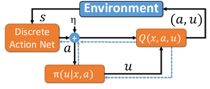
Figure 14: PASVG(0) (adapted from [wei2018hierarchical]).

6.5 Curriculum Learning

Curriculum learning (CL) approaches attempt to accelerate the learning process through initially subjecting the RL agent to a simplified version of the problem, and subsequently gradually increasing the task complexity, e.g., via a progression function  [bassich2019continuous, bassich2020curriculum]. This approach has also been applied to RL for combinatorial action spaces. [pmlr-v119-farquhar20a] introduce a CL approach using a growing action space (GAS). For an MDP with unrestricted action space $\mathcal{A}$ the authors define a set of $N$ action spaces $\mathcal{A}_{l},l\in\{0,...,N-1\}$. Each action space is a subset of the next level $l$: $\mathcal{A}_{0}\subset\mathcal{A}_{1}\subset...\subset\mathcal{A}_{N-1}\subset\mathcal{A}$. A policy restricted to an action space $\mathcal{A}_{l}$ is denoted as $\pi_{l}(a,s)$. The optimal policy for this restricted policy class is $\pi^{*}_{l}(u,x)$, and the corresponding action-value and value functions are: $Q^{*}_{l}(s,a)$ and $V^{*}_{l}(s)=\max_{a}Q^{*}_{l}(s,a)$. Domain knowledge is used to define a hierarchy of actions. For every action $a\in\mathcal{A}_{l}$ where $l>0$ there is a parent action $\texttt{parent}_{l}(a)$ in the space of $\mathcal{A}_{l-1}$. Given that at each level, subsets of action spaces are subsets of larger action spaces, the actions available in $\mathcal{A}_{l-1}$ are their own parents in $\mathcal{A}_{l}$. The authors note that in many environments Euclidean distances are a valid measure for implementing a heuristic for defining a hierarchy over actions.

An ablation study on discretized Acrobat and Mountaincart environments shows the value of efficiently using the data collected during training across levels. The authors also evaluate their approach on SMAC, using a far larger number of units compared to those usually used in MARL experiments – i.e., scenarios with 50-100 instead of 20-30. In addition, the task difficulty is increased through having randomized starting positions, and scripted opponent logic that holds its position until any agent-controlled unit is in range. Subsequently the enemy focus-fires on its closest enemy. Having to locate the enemy first increases the exploration challenge. The authors demonstrate the advantage of their approach GAS(2) (GAS with 2 levels) against various ablations of their approach and methods that directly train on the full action space.

[yu4167820curriculum] take a similar approach to GAS [pmlr-v119-farquhar20a] for decision making in intelligent healthcare. A Progressive Action Space (PAS) approach allows the learner to master easier tasks first, via generalized actions, before gradually increasing the granularity, e.g., modifying the precise volume of a drug to be given to a patient. This work focuses on an offline RL setting, where traditional approaches lead to inaccurate state-action evaluation for those actions seldom applied by the physicians in the historical clinical dataset – a common problem for offline RL [fujimoto2019off]. Similar to GAS [pmlr-v119-farquhar20a], PAS also requires domain knowledge for defining $N$ abstracted action spaces $\{a_{1},a_{2},...,a_{N}\}$ and a corresponding number of curricula $\{M_{1},M_{2},...,M_{N}\}$. Value and policy transfer approaches are used to transfer knowledge across levels.

7 Adversarial Learning

A number of approaches discussed in the previous sections have been applied to adversarial domains, including ACO (e.g., Wolpertinger [nguyen2020multiple] and CRLA [tran2022cascaded]). However, these approaches were trained against stationary opponents. In practice, the ACO problem is non-stationary, with Red and Blue adjusting their approach over time. In adversarial learning terminology, Red and Blue will attempt to compute approximate best responses (ABRs) to each others’ policies [oliehoek2018beyond].

7.1 The Adversarial Learning Challenge

In this section we shall formally define the adversarial learning problem, desirable solution concepts, and the approaches designed to help learning agents converge upon policies that are hard to exploit. ACO environments are adversarial. However, they are not always zero-sum games. For instance, in CAGE Challenge 2 Blue receives a penalty for restoring a compromised host due to the action having consequences for any of the Green agents currently working on this facility. Here, Red does not receive a corresponding reward $r_{Red}=-r_{Blue}$. Therefore, ACO lacks a key property from two player zero-sum games, where the gain of one player is equal to the loss of the other player. However, in this section we shall treat the ACO problem as a quasi zero-sum game, with the assumption that the consequences of Red winning outweigh other factors, shall assume: ${\mathcal{G}}_{1}({\pi,\mu})\approx-{\mathcal{G}}_{2}({\pi,\mu})$. An equilibrium concept commonly used in this class of games to define solutions is the Nash equilibrium [nash1951non]:

Definition 7.1 (Nash Equilibrium).

A joint policy $\bm{\pi}^{*}$ is a Nash equilibrium iff no player $i$ can improve their gain through unilaterally deviating from $\bm{\pi}^{*}$:

$$\forall i,\forall\pi_{i}\in\Delta(\mathcal{S},\mathcal{A}_{i}),\forall s\in\mathcal{S},{\mathcal{G}}_{i}(\langle\pi^{*}_{i},\bm{\pi}^{*}_{-i}\rangle)\geq{\mathcal{G}}_{i}(\langle\pi_{i},\bm{\pi}^{*}_{-i}\rangle).$$ (4)

Our focus is on finite two-player (quasi) zero-sum games, where an equilibrium is referred to as a saddle point, representing the value of the game $v*$. Given two policies $\pi_{1}$, $\pi_{2}$, the equilibria of a finite zero-sum game is:

Theorem 1 (Minmax Theorem).

In a finite zero-sum game:

$$max_{\pi_{1}}min_{\pi_{2}}{\mathcal{G}}_{i}(\langle\pi_{1},\pi_{2}\rangle)=min_{\pi_{2}}max_{\pi_{1}}{\mathcal{G}}_{i}(\langle\pi_{1},\pi_{2}\rangle)=v^{*}.$$ (5)

Above is one of the fundamental theorems of game theory, which states that every finite, zero-sum, two-player game has optimal mixed strategies [v1928theorie]. We shall discuss the implications of the above equations for ACO from the perspective of Blue. Given a joint-policy $\langle\pi^{*}_{Blue},\pi^{*}_{Red}\rangle$ where $\pi^{*}_{Blue}$ and $\pi^{*}_{Red}$ represent optimal mixed strategies, then by definition Red will be unable to learn a new best response $\pi_{Red}$ that improves on $\pi^{*}_{Red}$. Obtaining $\pi^{*}_{Blue}$ guarantees that Blue will perform well, even against a worst case opponent [perolat2022mastering]. This means that, even if the value of the game $v^{*}$ is in Red’s favour, assuming that Blue has found $\pi^{*}_{Blue}$, then Blue has found a policy that limits the extent to which that Red can exploit Blue.

One of the long-term objectives of MARL is to limit the exploitability of agents deployed in competitive environments [lanctot2017unified, oliehoek2018beyond, heinrich2016deep]. While a number of methods for limiting exploitability exist that are underpinned by theoretical guarantees, in practice finding the value of the game is challenging even for simple games. This is due to DRL using function approximators that are unable to compute exact best responses to an opponent’s policy. The best a DRL agent can achieve is an ABR. In addition, for complex games finding a Nash equilibrium is intractable. Here the concept of an approximate Nash equilibrium ($\epsilon$-NE) is helpful [oliehoek2018beyond, lanctot2017unified]:

Definition 7.2 ($\epsilon$-Nash Equilibrium).

The joint-policy $\bm{\pi}^{*}$ is an $\epsilon$-NE iff:

$$\forall i,\forall\pi_{i}\in\Delta(\mathcal{S},\mathcal{A}_{i}),\forall s\in\mathcal{S},{\mathcal{G}}_{i}(\langle\pi^{*}_{i},\bm{\pi}^{*}_{-i}\rangle)\geq{\mathcal{G}}_{i}(\langle\pi_{i},\bm{\pi}^{*}_{-i}\rangle)-\epsilon.$$ (6)

7.2 Approaches Towards Limiting Exploitability

The above raises the question: how can we efficiently limit the exploitability of ACO agents? A key insight here from the adversarial learning literature is that finding $\pi^{*}_{Blue}$ will require learning to best respond to principled Red agents, ideally through computing a best response against $\pi^{*}_{Red}$. However, similarly Red will need to face strong Blue agents to find $\pi^{*}_{Red}$. This raises the need for an iterative adversarial learning process where Blue and Red learn (A)BRs to each others’ latest policies. However, naïve independent learning approaches fail to generalize well due to a tendency to overfit on their opponents, also known as joint-policy correlation [lanctot2017unified]. Therefore, a more principled approach is required.

[gleave2019adversarial] show that an adversary can learn simple attack policies that reliably win against a static opponent implemented with function approximators. Often random and uncoordinated behavior is sufficient to trigger sub-optimal actions . By adversarial attacks the study refers to attacks on the opponents observation space. This is quasi equivalent to adding perturbations to images for causing a misclassification in supervised learning, but doing so via taking actions within the environment. A worrying finding is that DNNs are more vulnerable towards high-dimensional adversarial samples [gilmer2018adversarial, khoury2018geometry, shafahi2018adversarial]. The same applies for DRL. Empirical evaluations on MuJoCo show that the greater the dimensionality of the area of the observation space that Red can impact, the more vulnerable the victim is towards attacks [gleave2019adversarial].

The work by [gleave2019adversarial] shows that agents trained via simplistic training schemes – e.g., self-play – are very far from an $\epsilon$ bounded Nash equilibrium. This raises the need for training schemes designed to limit the exploitability of agents. [perolat2022mastering] identify three categories of approaches for reducing the exploitability of agents: regret minimization, regret policy gradient methods, and best response techniques.

The first category includes approaches that scale counterfactual regret minimization (CFR) using deep learning. Deep-CFR [brown2019deep] trains a regret DNN via an experience replay buffer containing counterfactual values. A limitation of this approach is the sampling method, in that it does not scale to games with a large branching factor [perolat2022mastering]. There are model-free regret-based approaches which use DNNs that scale to larger games, such as deep regret minimization with advantage baselines and model-free learning (DREAM) [steinberger2020dream] and the advantage regret-matching actor-critic (ARMAC) [gruslys2020advantage]. However, these approaches rely on an importance sampling term in order to remain unbiased. The importance weights can become very large in games with a long horizon [perolat2022mastering]. To generalize, these techniques require the generation of an average strategy, necessitating either the complete retention of all strategies from previous iterations, or an error prone approximation, e.g., a DNN trained via supervised learning [perolat2022mastering].

The second category of methods approximates CFR via a weighted policy gradient [srinivasan2018actor, perolat2022mastering]. However, the approach is not guaranteed to converge to a Nash equilibrium [perolat2022mastering]. In contrast Neural Replicator Dynamics (NeuRD) [hennes2019neural], an approach that approximates the Replicator Dynamics from evolutionary game theory with a policy gradient, is proven to converge to a Nash equilibrium. NeuRD has been applied to large-scale domains, as part of DeepNash [perolat2022mastering]. It is used to modify the loss function for optimizing the Q-function and the policy [perolat2022mastering]. DeepNash was recently introduced as a means of tackling the game of Stratego. However, its wider applicability is yet to be explored. In the remainder of this section we shall therefore focus on the third category of approaches: best response techniques.

7.3 Best Response Techniques

In recent years a number of principled approaches from the MARL literature – originally designed for competitive games with a low-dimensional state space – have been scaled to deep MARL. Population-based and game-theoretic training regimes have shown a significant amount of potential [li2023combining]. Early work in this area by [heinrich2016deep] scaled Fictitious Self-Play for domains suffering from the curse-of-dimensionality, resulting in Neural Fictitious Self-Play (NFSP). This approach approximates extensive-form fictitious play by progressively training a best response against the average of all past policies using off-policy DRL. A DNN is trained using supervised learning to imitate the average of the past best responses.

[lanctot2017unified] introduced Policy-Space Response Oracles (PSRO), a generalization of the Double-Oracle (DO) approach originally proposed by [mcmahan2003planning], a theoretically sound approach for finding a minimax equilibrium. Given the amount of interest that this approach has generated within the literature [berner2019dota, perolat2022mastering, vinyals2019grandmaster, lanctot2017unified, li2023combining, oliehoek2018beyond], we shall dedicate the remainder of this section to DO based approaches. First we will discuss the DO approach’s theoretical underpinnings, before providing an overview of the work that has been conducted in this area in recent years. We shall conclude the section with open challenges, in particular with respect to scaling this approach to ACO.

The DO algorithm defines a two-player zero-sum normal-form game $\mathcal{N}$, where actions correspond to policies available to the players within an underlying stochastic game $\mathcal{M}$. Payoff entries within $\mathcal{N}$ are determined through computing the gain $\mathcal{G}$ for each policy pair within $\mathcal{M}$:

$$\mathcal{R}^{\mathcal{N}}_{i}(\langle a^{r}_{1},a^{c}_{2}\rangle)=\mathcal{G}^{\mathcal{M}}_{i}(\langle\pi^{r}_{1},\pi^{c}_{2}\rangle).$$ (7)

In Equation 7, $r$ and $c$ refer to the respective rows and columns inside the normal-form (bimatrix) game, and $\mathcal{M}$ is the game where the policies are being evaluated. The normal-form game $\mathcal{N}$ is subjected to a game-theoretic analysis, to find an optimal mixture over actions for each player. These mixtures represent a probability distribution over policies for the game $\mathcal{M}$. The DO algorithm assumes that both players have access to a best response oracle, returning a best response (BR) policy against the mixture played by the opponent. BRs are subsequently added to the list of available policies for each agent. As a result each player has an additional action that it can choose in the normal-form game $\mathcal{N}$. Therefore, $\mathcal{N}$ needs to be augmented through computing payoffs for the new row and column entries. Upon augmenting $\mathcal{N}$ another game theoretic analysis is conducted, and the steps described above are repeated. If no further BRs can be found, then the DO algorithm has converged upon a minimax equilibrium [mcmahan2003planning].

When applying the DO algorithm to MARL the oracles must compute Approximate Best Responses (ABRs) against a mixture of policies. There are a number of approaches for implementing a mixture of policies, e.g., sampling individual policies according to their respective mixture probabilities at the beginning of an episode [lanctot2017unified]. Alternatively, the set of policies can be combined into a weighted-ensemble, where the outputs from each policy are weighted by their respective mixture probabilities prior to aggregation. For generality, we define a mixture of policies as follows:

Definition 7.3 (Mixture of Policies).

$\pi_{i}^{\mu}$ is a mixture of policies for a mixture $\mu_{i}$ and a corresponding set of policies $\Pi_{i}$ for agent $i$.

Using an oracle to obtain an exact best response is often also intractable. In games that suffer from the curse-of-dimensionality an oracle can at best hope to find an ABR [oliehoek2018beyond]. Here we can apply Approximate Double-Oracles (ADO), which use linear programming to compute an approximate mixed-strategy NE $\langle{\mu}_{1},{\mu}_{2}\rangle$ for $\mathcal{N}$, where ${\mu}_{i}$ represents a mixture over policies $\pi_{i,1..n}$ for player $i$. We therefore require a function $O:\Pi_{i}^{\mu}\rightarrow\Pi_{i}$ that computes an ABR $\pi_{i}$ to a mixture of policies $\pi_{i}^{\mu}$:

Definition 7.4 (Approximate Best Response).

A policy $\pi_{i}\in\Pi_{i}$ of player $i$ is an approximate best response against a mixture of policies $\pi_{j}^{\mu}$, iff,

$$\forall\pi^{\prime}_{i}\in\Pi_{i},{\mathcal{G}}_{i}(\langle\pi_{i},\pi^{\mu}_{j}\rangle)\geq{\mathcal{G}}_{i}(\langle\pi^{\prime}_{i},\pi_{j}^{\mu}\rangle).$$ (8)

ABRs estimate the exploitability $\mathcal{G}_{E}$ of the current mixtures:

$$\mathcal{G}_{E}\leftarrow{\mathcal{G}}_{i}(\langle{O}_{i}(\pi^{\mu}_{j}),\pi^{\mu}_{j}\rangle)+{\mathcal{G}}_{j}(\langle\pi^{\mu}_{i},{O}_{j}(\pi^{\mu}_{i})\rangle)$$ (9)

If $\mathcal{G}_{E}\leq 0$, then the oracle has failed to find an ABR, and a resource bounded Nash equilibrium (RBNE) has been found [oliehoek2018beyond]. Resources in this context refers to the amount of computational power available for obtaining an ABR:

Definition 7.5 (Resource Bounded Nash Equilibrium).

Two mixtures of policies $\langle\pi^{\mu}_{1},\pi^{\mu}_{2}\rangle$ are a resource-bounded Nash equilibrium (RBNE) iff,

$$\forall_{i}{\mathcal{G}}_{i}(\langle\pi^{\mu}_{i},\pi^{\mu}_{j}\rangle)\geq{\mathcal{G}}_{i}(\langle{O}_{i}(\pi^{\mu}_{j}),\pi^{\mu}_{j}\rangle).$$ (10)

Each agents’ oracle is unable to find a response that outperforms the current mixture of policies against the opponent’s one. Therefore, an RBNE has been found. The ADO approach is outlined in Algorithm 2 from the perspective of Blue and Red agents for ACO. The algorithm makes use of a number of functions, including i.) InitialStrategies, for providing an initial set of strategies for each agent, which can also include rules-based and other approaches; ii.) AugmentGame, that computes missing table entries for the new resource bounded best responses, and; iii.) SolveGame, for computing mixtures once the payoff table has been augmented [oliehoek2018beyond].

Algorithm 2 Approximate Double Oracle Algorithm

1:$\langle{\pi}_{Blue},{\pi}_{Red}\rangle\leftarrow\textsc{InitialStrategies}()$

2:$\langle{\mu}_{Blue},{\mu}_{Red}\rangle\leftarrow\langle\{{\pi}_{Blue}\},\{{\pi}_{Red}\}\rangle$ $\triangleright$ set initial mixtures

3:while True do

4:    ${\pi}_{Blue}\leftarrow\textsc{RBBR}({\mu}_{Red})$ $\triangleright$ get new res. bounded best resp.

5:    ${\pi}_{Red}\leftarrow\textsc{RBBR}({\mu}_{Blue})$

6:    $\mathcal{G}_{RBBRs}\leftarrow{\mathcal{G}}_{Blue}({\pi}_{Blue},{\mu}_{Red})+{\mathcal{G}}_{Red}({\mu}_{Blue},{\pi}_{Red})$ $\triangleright$ Exploitability.

7:    if $\mathcal{G}_{RBBRs}\leq\epsilon$ then

8:         break $\triangleright$ found $\epsilon$-RBNE

9:    end if

10:    $SG\leftarrow\textsc{AugmentGame}(SG,{\pi}_{Blue},{\pi}_{Red})$

11:    $\langle{\mu}_{Blue},{\mu}_{Red}\rangle\leftarrow\textsc{SolveGame}(SG)$

12:end while

7.4 Towards Scaling Adversarial Learning Approaches

Versions of ADO have been used at scale, e.g., [vinyals2019grandmaster] achieve a grandmaster level performance in StarCraft II, beating top human players using AlphaStar, an ADO inspired approach that computes best responses using a match-making mechanism that samples strong opponents with an increased probability. Imitation learning was utilized to obtain an initial pool of agents. OpenAI Five made use of similar mixture of self-play method and a dynamically-updated meta-distribution over past policies, beating top human players at Dota [berner2019dota, perolat2022mastering]. Both achievements, although very impressive, come at a high cost with respect to engineering and training time. Indeed, despite their success, questions remain regarding the scalability of ADO to complex domains without making concessions at the cost of theoretical guarantees. ADO approaches are expensive due to:

Computing ABRs in non-trivial environments is a lengthy process [lanctot2017unified]. Meanwhile, even for simple environments such as Kuhn poker, ADO can require over 20 ABR iterations to approach the value of the game. For the slightly more complex Leduc this number grows to over 200, with further improvements still being obtainable [lanctot2017unified, li2023combining]. An even larger number of iterations would likely be necessary for ADO to approach $\pi^{*}_{Blue}$ for ACO. Computing ABRs from scratch in each iteration would therefore be wasteful, especially if the same skills are learnt from scratch in each iteration [liuneupl]. In addition, due to the ABRs being resource bounded [oliehoek2018beyond], each agent can end up with a population of under-trained policies [liuneupl]. An idealized ADO reuses relevant knowledge acquired over past iterations.

Payoff Matrix Augmentation. The second challenge with respect to scalability is the growing normal-form game $\mathcal{N}$. Augmenting the payoff table with entries for new best responses takes exponential time with respect to the number of policies [lanctot2017unified]. Even for simple games, obtaining a good payoff estimate for each ${\mathcal{G}}_{i}(\langle\pi^{r}_{i},\pi^{c}_{j}\rangle)$ can require thousands of evaluation episodes. Principled strategies are required for keeping the payoff tables to a manageable size.

Large Policy Supports. There is an overhead for having to store and utilize a large number of function approximators – one for each policy in the support [ijcai2019-66].

While the above challenges limit the scalability of ADO, there have been efforts towards remedying this approach without harming too many of the underlying principles. [liuneupl] propose Neural Population Learning (NeuPL) a method that deviates from the standard ADO algorithm PSRO in two specific ways: i.) all unique policies within the population are trained continuously, and; ii.) uses a single policy that contains the entire population of policies, conditioned on an opponent mixture identifier. This allows for learning to be transferred across policies without a loss of generality. The approach is capable of outperforming PSRO while maintaining a population of eight agents on running-with-scissors, which extends the rock-paper-scissors game to the spatio-temporal and partially-observed Markov game [vezhnevets2020options].

It is also worth noting that the benefits of PSRO have been explored within single agent domains, specifically within the context of robust adversarial reinforcement learning (RARL) [pinto2017robust]. For RARL a single agent environment is converted into a zero-sum game between the standard agent, the protagonist, and an adversarial domain agent, that can manipulate the environment, e.g., through perturbing the protagonist’s actions. [yang2022game] recently applied a variant of PSRO to this problem, using model agnostic meta learning (MAML) [finn2017model] as the best-response oracle. The authors conducted an empirical evaluation on MuJoCo environments, finding that the proposed method outperforms state-of-the-art baselines such as standard MAML [yang2022game].

ADO has also been applied to general-sum games, which can have more than one Nash equilibrium. This gives rise to the equilibrium selection problem. To remedy this, and enable scalable policy evaluation in general, [muller2020generalized] apply the $\alpha$-Rank solution concept, which does not face an equilibrium selection problem. The $\alpha$-Rank solution concept establishes an ordering over policies within the support of each player. Specifically, $\alpha$-Rank uses Markov-Conley Chains to identify the presence of cycles in game dynamics, and thereby rank policies. The approach attempts to compute stationary distributions by evaluating the strategy profiles of $N$ agents through an evolutionary process of mutation and selection. [yang2020alphaalpha] reviewed the claim of $\alpha$-ranks tractability. The authors find that instead of being a polynomial time implementation, (with respect to the total number of pure strategy profiles) solving $\alpha$-Rank is NP-hard. The authors introduce $\alpha^{\alpha}$-Rank, a stochastic implementation of $\alpha$-Rank that does not require an exponentially-large transitions matrix for ranking policies, and can terminate early.

[feng2021neural] replace the computation of mixtures using linear-programming with a Neural Auto-Curricula (NAC), using meta-gradient descent to automate the discovery of the learning update rules (the mixtures) without explicit human design. The NAC is optimized via interaction with the game engine, where both players aim to minimise their exploitability. Even without human design, the discovered MARL algorithms achieve competitive or even better performance with the SOTA population-based game solvers on a number of benchmarking environments, including: Games of Skill, differentiable Lotto, non-transitive Mixture Games, Iterated Matching Pennies, and Kuhn Poker. However, the approach does not solve scalability issues with respect to the increase in time for augmenting the payoff tables, and the time required for computing ABRs.

Finally, we note that DO based methods have also been utilized for reducing the number of actions for an agent to choose from, given a state $s$ in two player games. [bakhtin2021no] propose an ADO based algorithm for action exploration and equilibrium approximation in games with combinatorial action spaces: Double Oracle Reinforcement learning for Action exploration (DORA). This algorithm simultaneously performs value iteration while learning a policy proposal network. An ADO step is used to explore additional actions to add to the policy proposals. The authors show that their approach achieves superhuman performance on a two-player variant of the board game Diplomacy.

8 Discussion and Open Questions

The previous sections provide a comprehensive overview of the plethora of methods for addressing high-dimensional states, large combinatorial action spaces and reducing the exploitability of DRL agents. We shall now consider how the lessons learned from this process can help us formulate an idealised learner for ACO, and distill open research questions.

The need for improved evaluation metrics: After reading sec:adv_learning, it should be evident that success achieved against a stationary opponent should be enjoyed with caution. For example, for the CAGE challenges [cage_challenge_announcement, cage_challenge_2_announcement, cage_challenge_3_announcement], the evaluation process to-date has consisted of evaluating the submitted approach against rules-based Red agents with different trial lengths. This formulation is concerning. Solutions that overfit on the provided Red agents are likely to perform best. To address this shortcoming we advocate for exploitability being used as a standard evaluation metric, given that it is widely used by the adversarial learning community [lanctot2017unified, oliehoek2018beyond, heinrich2016deep], raising the research question:

Q1:

How exploitable are current approaches for autonomous cyber operations?

The need for improved evaluation environments: In sec:envs, it is identified that the challenges which would be present in an idealised ACO training environment are not currently implemented in CybORG or YAWNING TITAN. While environments are available to benchmark subsets of these challenges, no environment can be used to benchmark all of them. In particular, although RecSim and Micro-RTS are available to benchmark high-dimensional observation and action spaces, respectively, no environment is available to pose these challenges alongside graph-based dynamics. Practitioners aiming to develop methodologies which rely on graph constructs specifically have several avenues for environment development, with two open-source but difficult to modify ACO environments being available, alongside frameworks such as Gym-ANM which are designed to be built upon. As such, the following research (and development) questions arise:

Q2:

Will methodologies developed on environments such as RecSim and Micro-RTS translate well to ACO?

Q3:

Where should environment developers seeking to build towards a more idealised graph-based ACO-like environment focus their efforts?

Limiting the exploitability of cyber defence agents: Handcrafting world-beating rules-based agents that find the value of the game is non-trivial, even for simple games [vincent2021top]. Therefore, our thoughts turn towards adversarial learning approaches for ACO. We have seen that best response techniques have a significant amount of potential. However, while computing an (approximate) best response to measure exploitability is a reasonable expenditure, best response techniques require this in every iteration. As a result the literature on adversarial learning often focuses on simple games for benchmarking such as Kuhn and Leduc poker, where the value of the game is known [lanctot2019openspiel, feng2021neural, li2023combining, lanctot2017unified]. Meanwhile, methods that we have identified as suitable for ACO can require lengthy training times. This raises the following research questions:

Q4:

Can we implement an efficient best response framework for cyber defence?

Q5:

What is the value of the game for non-trivial cyber defence configurations?

Efficient approximate best response oracles: While RQ4 focuses on mechanisms within the approximate best response framework to reduce training time (e.g., through knowledge reuse [liuneupl]), the endeavour is underpinned by the need for methods that themselves can be trained efficiently. However, this is not a property one would associate with the methods discussed in sections 5 and 6, raising the question:

Q6:

Can we implement wall time efficient best response oracles for ACO?

9 Conclusions

In this work we surveyed the DRL literature to formulate an idealised learner for autonomous cyber operations. This idealised learner sits at the intersection of three active areas of research, namely environments that confront learners with the curse of dimensionality, with respect to both state and action spaces, and adversarial learning. While significant efforts have been made on each of these topics individually, each still remains an active area of research.

While SOTA DNNs have allowed RL approaches to be scaled to domains that were previously considered high-dimensional [mnih2013playing, mnih2015human], in this survey we provide an overview of solutions for environments that push standard DRL approaches to their limits. In sections 5 – 7 we identify components for the implementation and evaluation of an idealised learning agent for ACO, and in sec:challenges we discuss both theoretical and engineering challenges that need to be overcome in-order to: implement our idealised agent, and; train it at scale. We hope that this survey will raise awareness regarding issues that need to be solved in-order for DRL to be scalable to challenging cyber defence scenarios, and that our work will inspire readers to attempt to answer the research questions we have distilled from the literature.

10 Acknowledgements

Research funded by Frazer-Nash Consultancy Ltd. on behalf of the Defence Science and Technology Laboratory (Dstl) which is an executive agency of the UK Ministry of Defence providing world class expertise and delivering cutting-edge science and technology for the benefit of the nation and allies. The research supports the Autonomous Resilient Cyber Defence (ARCD) project within the Dstl Cyber Defence Enhancement programme.

11 License

This work is licensed under the Creative Commons Attribution-NonCommercial-NoDerivatives 4.0 International License. To view a copy of this license, visit https://creativecommons.org/licenses/by-nc-nd/4.0/ or send a letter to Creative Commons, PO Box 1866, Mountain View, CA 94042, USA.

12 Deep Reinforcement Learning

12.1 Deep Q-Learning

In DRL multi-layer Deep Neural Networks (DNNs) are used to approximate value functions or, as we shall see below, even learn a parameterized policy. We shall assume a DNN with parameters $\theta$ and sufficient representational capacity to learn our required approximations. For Deep Q-learning (DQN), DNNs map a set of $n$-dimensional state variables to a set of $m$-dimensional Q-values $f:\mathbb{R}^{n}\to\mathbb{R}^{m}$ [mnih2013playing, mnih2015human]. Here, $m$ represents the number of actions available to the agent. The parameters $\theta$ are optimized via stochastic gradient descent, by randomly sampling past transitions stored within an experience replay memory $\mathcal{D}$ [lin1992self, mnih2015human, schaul2015prioritized, mousavi2016deep]. The DNN is trained to minimize the time dependent loss function,

$$L_{k}\left(\theta_{k}\right)=\mathbb{E}_{(s,a,s^{\prime},r)\sim U(\mathcal{D})}\Big{[}\left(Y_{k}-Q\left(s,a;\theta_{k}\right)\right)^{2}\Big{]},$$ (11)

where $(s,a,s^{\prime},r)\sim U(\mathcal{D})$ represents mini-batches of experiences drawn uniformly at random from $\mathcal{D}$, $t$ the current iteration, and $Y_{k}$ is the target:

$$Y_{k}\equiv r+\gamma Q(s^{\prime},\operatorname*{argmax}_{a\in\mathcal{U}}Q(s^{\prime},a;\theta_{k});\theta_{k}^{\prime}).$$ (12)

Equation (12) uses Double Deep Q-learning (DDQN) [hasselt2010double], where the target action is selected using weights $\theta$, while the target value is computed using weights $\theta^{\prime}$ from a target network. Using the current network rather than the target network for the target value estimation decouples action selection and evaluation for more stable updates. Weights are copied from the current to the target network after every $n$ transitions [van2016deep] or via a soft target update  [lillicrap2015continuous]. DDQNs have been shown to reduce overoptimistic value estimates [van2016deep].

12.2 Proximal Policy Optimisation

While laying important foundations, DQNs tend to be outperformed by SOTA policy gradient (PG) methods, such as Proximal Policy Optimization (PPO) [schulman2017proximal]. PG approaches optimize a parameterized policy $\pi_{\theta}$ directly. The objective is to find an optimal policy $\pi^{*}_{\theta}$ with respect to the parameters $\theta$, which maximizes the expected return $J(\theta)=\mathbb{E}_{x_{i}\sim p_{\pi},a_{i}\sim\pi}[\mathcal{R}_{0}]$. PPO gathers $(s_{t},a_{t},r_{t},s_{t+1},a_{t+1},r_{t+1},...,s_{t+n},a_{t+n},r_{t+n})$ trajectories by interacting with the environment, potentially over multiple instances of the environment using multiple actors synchronously or asynchronously [mnih2016asynchronous]. The collected samples are then used to update the policy for a number of epochs, upon which the collected data is discarded. Then, a new iteration of collecting data for updating the policy begins, making the algorithm on policy. The policy is optimized through estimating the PG and subsequently running a stochastic gradient ascent algorithm:

$$\hat{g}=\mathbb{\hat{E}}_{t}\Big{[}\nabla_{\theta}\log\pi_{\theta}(a_{t}\rvert s_{t})\hat{A}_{t}\Big{]}.$$ (13)

In the above equation $\hat{A}_{t}$ is an estimate of the advantage function at time step $t$. The advantage function is computed using a learned state-value function $V(s)$, resulting in an actor-critic style architecture. The expectation $\mathbb{\hat{E}}_{t}[...]$ represents the fact that an empirical average over a finite batch of samples is used for computing the gradient. Therefore, as mentioned above, we assume an algorithm that alternates between sampling and updating the policy parameters $\theta$:

$$L^{PG}(\theta)=\mathbb{\hat{E}}_{t}\Big{[}\log\pi_{\theta}(a_{t}\rvert s_{t})\hat{A}_{t}\Big{]}.$$ (14)

Performing multiple optimization steps on this loss, i.e., using the same trajectory, can lead to destructively large policy updates. To address this, PPO uses a a clipped surrogate loss function that effectively constrain the size of each update, allowing multiple epochs of mini-batch updates to be performed on gathered data. Given a probability ratio

$${}_{t}(\theta)=\dfrac{\pi_{\theta}(a_{t}\rvert s_{t})}{\pi_{\theta_{old}}(a_{t}\rvert s_{t})},$$ (15)

PPO prevents $\theta$ from moving too far away from $\theta_{old}$:

$$L^{CLIP}(\theta)=\mathbb{\hat{E}}_{t}\Big{[}min({}_{t}(\theta)\hat{A}_{t},clip({}_{t}(\theta),1-\varepsilon,1+\varepsilon)\hat{A}_{t})\Big{]}.$$ (16)

12.3 Deep Deterministic Policy Gradients

For continuous control problems, the policy can also be updated by taking the gradient of the expected return. A popular actor-critic method is Deep Deterministic Policy Gradients (DDPG) [lillicrap2015continuous] which uses many of the same fundamental principles of DQN but applied to continuous control problems. An actor $\mu(s)$ with network parameters $\phi$ is used for action selection, while the critic $Q(s,a)$ with network parameters $\theta$ provides the value function estimate. The critic is updated using temporal difference learning as with DQN in eq:DQNTarget, but the target value is estimated using the target actor and critic networks:

$$Y_{k}=r+\gamma\hat{Q}_{\hat{\theta}}\left(s^{\prime},\hat{\mu}_{\hat{\phi}}(s^{\prime})\right)$$ (17)

The actor network is then updated through gradient ascent using the deterministic policy gradient algorithm [silver2014deterministic]:

$$\nabla_{\phi}J_{k}(\phi)=\mathbb{E}\left[\nabla_{a}Q_{\theta}(s,a)\rvert_{a=\mu(s)}\nabla_{\phi}\mu_{\phi}(s)\right]$$ (18)

The target actor and critic networks are then updated using soft target updates.

13 High-Dimensional State Space Approaches Overview

Papers that are relevant with regard to the high-dimensional state spaces
Work	Summary	Abstr.	Expl.	CF
[pmlr-v80-abel18a]	Authors introduce two classes of abstractions: transitive and PAC state abstractions, and show that transitive PAC abstractions can be acquired efficiently, preserve near optimal-behavior, and experimentally reduce sample complexity in simple domains.	✓	X	X
[abel2016near]	Authors investigate approximate state abstractions, Present theoretical guarantees of the quality of behaviors derived from four types of approximate abstractions. Empirically demonstrate that approximate abstractions lead to reduction in task complexity and bounded loss of optimality of behavior in a variety of environments.	✓	✓	X
[abel2019state]	Seek to understand the role of information-theoretic compression in state abstraction for sequential decision making, resulting in a novel objective function.	✓	✓	X
[pmlr-v108-abel20a]	Combine state abstractions and options to preserve the representation of near-optimal policies.	✓	✓	X
[atkinson2021pseudo]	A generative network is used to generate short sequences from previous tasks for the DQN to train on, in order to prevent catastrophic forgetting as the new task is transferred.	X	X	✓
[badianever]	Construct an episodic memory-based intrinsic reward using k-nearest neighbours over recent experiences. Encourage the agent to repeatedly revisit all states in its environment.	X	✓	✓
[bellemare2016unifying]	Use Pseudo-Counts to count salient events, derived from the log-probability improvement according to a sequential density model over the state space.	✓	✓	X
[bougie2021fast]	Introduce the concept of fast and slow curiosity that aims to incentivise long-time horizon exploration. Method decomposes the curiosity bonus into a fast reward that deals with local exploration and a slow reward that encourages global exploration.	X	✓	X
[burdaexploration]	Introduce a method to flexibly combine intrinsic and extrinsic rewards via a random network distillation (RND) bonus enabling significant progress on several hard exploration Atari games.	X	✓	X
[burden2018using]	Automate the generation of Abstract Markov Decision Processes (AMDPs) using uniform state abstractions. Explores the effectiveness and efficiency of different resolutions of state abstractions.	✓	✓	X
[burden2021latent]	Introduce Latent Property State Abstraction, for the full automation of creating and solving an AMDP, and apply potential function for potential based reward shaping.	✓	✓	X
[pmlr-v97-gelada19a]	Introduce DeepMDP, where the $\ell_{2}$ distance represents an upper bound of the bisimulation distance, learning embeddings that ignore irrelevant objects that are of no consequence to the learning agent(s).	✓	✓	X
[colas2019curious]	Proposes CURIOUS, an algorithm that leverages a modular Universal Value Function Approximator with hindsight learning to achieve a diversity of goals of different kinds within a unique policy and an automated curriculum learning mechanism that biases the attention of the agent towards goals maximizing the absolute learning progress. Also focuses on goals that are being forgotten.	X	✓	✓
[de2015importance]	Study the extent to which experience replay memory composition can mitigate catastrophic forgetting.	X	X	✓
[precup2000temporal]	Introduction of the options framework, for prediction, control and learning at multiple timescales.	✓	✓	$\nearrow$
[fangadaptive]	Introduce Adaptive Procedural Task Generation (APT-Gen), an approach to progressively generate a sequence of tasks as curricula to facilitate reinforcement learning in hard-exploration problems.	X	✓	X
[forestier2017intrinsically]	Introduce an intrinsically motivated goal exploration processes with automatic curriculum learning.	✓	✓	X
[fu2017ex2]	Propose a novelty detection algorithm for exploration. Classifiers are trained to discriminate each visited state against all others, where novel states are easier to distinguish.	X	✓	X
[9287851]	Map high-dim video to a low-dim discrete latent representation using a VQ-AE.	✓	✓	X
[hester2013learning]	Focus on learning exploration in model-based RL.	X	✓	X
[kessler2022same]	Show that existing continual learning methods based on single neural network predictors with shared replay buffers fail in the presence of interference. Propose a factorized policy, using shared feature extraction layers, but separate heads, each specializing on a new task to prevent interference.	X	X	✓
[kovac2020grimgep]	Set goals in the region of highest uncertainty. Exploring uncertain states with regard to the rewards are the sub-goals.	✓	✓	X
[kulkarni2016hierarchical]	Introduce a hierarchical-DQN (h-DQN) operating at different temporal scales.	✓	✓	X
[dietterich2000overview]	An overview of the MAXQ value function decomposition and its support for state and action abstraction.	✓	✓	X
[machado2017laplacian]	Introduce a Laplacian framework for option discovery.	✓	✓	X
[machadoeigenoption]	Look at Eigenoptions, options obtained from representations that encode diffusive information flow in the environment. Authors extend the existing algorithms for Eigenoption discovery to settings with stochastic transitions and in which handcrafted features are not available.	✓	✓	X
[pmlr-v119-misra20a]	Authors introduce HOMER, an iterative state abstraction approach that accounts for the fact that the learning of a compact representation for states requires comprehensive information from the environment.	✓	✓	X
[martin2017count]	Count-based exploration in feature space rather than for the raw inputs.	✓	✓	X
[pathak2017curiosity]	Intrinsic rewards based method that formulates curiosity as the error in an agent’s ability to predict the consequence of its own actions in a visual feature space learned by a self-supervised inverse dynamics model.	✓	✓	X
[savinovepisodic]	Propose a new curiosity method which uses episodic memory to form the novelty bonus. Current observation is compared with the observations in memory.	✓	✓	X
[stadie2015incentivizing]	Evaluate sophisticated exploration strategies, including Thompson sampling and Boltzman exploration, and propose a new exploration method based on assigning exploration bonuses from a concurrently learned model of the system dynamics.	✓	✓	X
[ribeiro2019multi]	Train DRL on two similar tasks, augmented with EWC to mitigate catastrophic forgetting.	X	X	✓
[tang2017exploration]	Use an auto-encoder and SimHash for to enable count based exploration.	✓	✓	X
[vezhnevets2017feudal]	Introduce FeUdal Networks (FuNs): a novel architecture for hierarchical RL. FuNs employs a Manager module and a Worker module. The Manager operates at a slower time scale and sets abstract goals which are conveyed to and enacted by the Worker. The Worker generates primitive actions at every tick of the environment.	✓	✓	X
[zhanglearning]	Propose deep bisimulation for control (DBC). DBC learns directly on this bisimulation distance metric. Allows the learning of invariant representations that can be used effectively for downstream control policies, and are invariant with respect to task-irrelevant details.	✓	✓	X

Table 2: An overview of approaches for addressing the curse of dimensionality with regard to states, and the extent to which works cover the topics of abstraction, advanced exploration strategies, and the mitigation of catastrophic forgetting.