The tropical polytope is the set of all weighted tropical Fermat-Weber points

Abstract.

Let $v_{1},\ldots,v_{m}$ be points in $\mathbb{R}^{n}$, and let $w_{1},\ldots,w_{m}$ be positive real weights. The weighted Fermat-Weber points are those points $z$ which minimize $\sum w_{i}d(v_{i},z)$. Following Comăneci and Joswig, we study the weighted Fermat-Weber points with respect to an asymmetric tropical metric. In the unweighted case (when $w_{1}=\cdots=w_{m}=1$), Comăneci and Joswig showed that the set of Fermat-Weber points is the “central” cell of the tropical convex hull of $v_{1},\ldots,v_{m}$. We show that for any fixed data points $v_{1},\ldots,v_{m}$, as the weights $w_{i}$ vary, the set of all Fermat-Weber points is the entire tropical convex hull of the $v_{i}$.

1. Introduction

Phylogenetics is a field of computational biology concerned with converting molecular data into trees that capture evolutionary relationships. While there are several, often combinatorial, methods for computing these phylogenetic trees, typically there is much discrepancy among the various resulting trees. Thus, a key hurdle to overcome is to find a tree which best represents the true evolutionary data. A common strategy is to gather information from many trees and compile this information into a single tree. The resulting tree obtained from such a strategy is called a consensus tree and the algorithm used to compute a consensus tree is called a consensus method. Still there are many consensus methods for computing a consensus tree. For a survey of consensus methods see [1]. While many consensus methods are combinatorial, in this paper our approach is through tropical geometry.

A phylogenetic tree is a metric tree with $N$ leaves. We embed the set of phylogenetic trees on N leaves into $\mathbb{R}^{\binom{N}{2}}$, by sending a tree $T$ to the list of $\binom{N}{2}$ distances between each of the pairs of leaves of $T$. This space is known as the space of phylogenetic trees [8]. In this paper, we only consider trees up to adding a constant to all pendant (leaf-adjacent) edge lengths. In this setting, the space of phylogenetic trees can be realized as a tropical linear space, the space of ultrametrics, in the tropical projective torus $\mathbb{R}^{\binom{N}{2}}/\mathbb{R}\mathbbm{1}$ [8]. In particular, this tree space is tropically convex – for more background see [8, §4.3].

A problem of computing a consensus tree can now be stated as the following optimization problem: for a fixed set of points in phylogenetic tree space, locate a point which minimizes the sum of distances to that point. This type of problem is more broadly known as a Fermat-Weber problem. A Fermat-Weber problem is a geometric problem seeking the median of a collection of data points $v_{1},\ldots,v_{m}$ taken from a metric space $X$, specifically the problem asks to find a point $x$ such that sum $\sum_{i=1}^{m}d(x,v_{i})$ is minimized. Such a median $x$ is called a Fermat-Weber point. This optimization problem arises in many different contexts such as linear programming via transportation problems [2], economics via location theory [4], and of course phylogenetics via tropical geometry [2, 7].

In the Euclidean case, there is a single Fermat-Weber point, and it is contained in the convex hull of the data points. In [2], Comăneci and Joswig show that with an asymmetrical tropical metric on phylogenetic tree space, the Fermat-Weber points form a cell in the tropical convex hull of the data points. Since phylogenetic tree space is tropically convex, this means that each Fermat-Weber point can be interpreted as a tree itself.

Classically, the Fermat-Weber problem was first posed by Fermat before 1640 to compute the Fermat-Weber point when $P$ is a triangle in Euclidean space. It was solved geometrically by Evangelista Torricelli in 1645. We note that the sum $\sum_{i=1}^{m}d(x,v_{i})$ assumes that the distances are weighted equally. Motivated by unequal attracting forces on particles, a generalization of the problem was introduced and solved by Thomas Simpson in 1750, later popularized by Alfred Weber in 1909, by considering weighted distances. In that spirit, this paper is concerned with generalizing the result by Comăneci and Joswig, namely, we are interested in locating the specific cells for which the Fermat-Weber points live in $P$ by minimizing the sum $\sum_{i=1}^{m}w_{i}d(x,v_{i})$ for some choice of positive real weights $w_{i}$. Our main theorem states that the Fermat-Weber set is a cell of the tropical convex hull $P$ and that, by choosing weights appropriately, it can be any cell of $P$.

Theorem 1.1.

Given data points $v_{1},\ldots,v_{m}$, the collection of asymmetric tropical weighted Fermat-Weber points over all possible positive real weights $w_{i}$ is $P=\mathrm{tconv}\{v_{1},\ldots,v_{m}\}$.

This paper is organized as follows: in Section 2 we provide background in tropical geometry and polyhedral geometry necessary to understand our approach. Of particular interest we recall the Cayley trick which gives a correspondence between mixed subdivisions of the Minkowski sum of polytopes and subdivisions of the corresponding Cayley polytope. Further, at the end of Section 2 we formulate the Fermat-Weber problem in the language of tropical convexity. In Section 3, we prove our main result Theorem 1.1 as a corollary to Theorem 3.2.

2. Background

In this section we set up the framework of the Fermat-Weber problem and introduce the algebraic and geometric tools that we use to study it.

2.1. Classical Polytopes

In this subsection we recall objects from convex geometry that play keys roles in computing Fermat-Weber sets. A polyhedron $P\subset\mathbb{R}^{n}$ is an intersection of finitely many half spaces. We call $P$ a polytope if this intersection is bounded. In this case, we write $P=\mbox{conv}(A)$ to mean $P$ is the convex hull of some finite set $A\subset\mathbb{R}^{n}$. For instance the standard simplex is the convex hull of the $n$ standard basis vectors in $\mathbb{R}^{n}$ and we denote it by $\Delta^{n-1}$. A face of a polytope $P$ is the collection of points in $P$ that minimizes the dot product with a fixed vector $u$, specifically

(1) $$\mbox{face}_{\mathbf{u}}(P):=\{\mathbf{x}\in P\mid\mathbf{u}\cdot\mathbf{x}\leq\mathbf{u}\cdot\mathbf{y},\forall\mathbf{y}\in P\}.$$

A polyhedral complex is a collection of polyhedra $S=\{C_{i}\}$ with the following properties: (1) $S$ is closed under taking faces, and (2) $C_{i}\cap C_{j}$ is a face of both $C_{i}$ and $C_{j}$, or is empty. The normal cone to $F$ in $P$, denoted $\sigma_{F}$, is the set of all vectors $u\in\left(\mathbb{R}^{m}\right)^{\ast}$ such that $\mbox{face}_{\mathbf{u}}(P)\supseteq F$. Alternatively, $\sigma_{F}$ is the closure of $\{u\in\left(\mathbb{R}^{m}\right)^{\ast}\mid\mbox{face}_{\mathbf{u}}(P)=F\}$. The normal fan of a polytope $P$ is the collection of cones $\{\sigma_{F}\}_{F\text{ a face of }P}$.

For the remainder of this section we are concerned with subdivisions of polytopes. Consider $m$ polytopes $P_{1},\ldots,P_{m}\subset\mathbb{R}^{n}$ where $P_{i}=\mathrm{conv}(A_{i})$ for some finite sets $A_{i}\subset\mathbb{R}^{n}$. A subdivision of a polytope $P$ is a polyhedral complex $S=\{C_{i}\}$ such that $P=\bigcup_{i}C_{i}$.

Definition 2.1.

Given a polytope $P=\mbox{conv}\{\mathbf{v}_{1},\ldots,\mathbf{v}_{k}\}\subset\mathbb{R}^{n}$, and weights $w_{i}\in\mathbb{R}$ on $\mathbf{v}_{i}$, the lift of $P$ with respect to $\mathbf{w}$ is

(2) $$\tilde{P}:=\mbox{conv}\{(\mathbf{v}_{i},w_{i})\mid i=1,\ldots,k\}\subset\mathbb{R}^{n+1}$$

A face $F=\mbox{face}_{\mathbf{u}}(\tilde{P})$ of $\tilde{P}$ is an upper face if $u_{n+1}<0$. The regular subdivision of $P$ with respect to $\mathbf{w}$ is the projection of the upper faces of $\tilde{P}$ onto $P$ (forgetting the last coordinate). An example is given in Example 2.24.

Definition 2.2.

The normal complex of a regular subdivision is the projection of the cones of the normal fan of $\tilde{P}$ that are normal to upper faces of $\tilde{P}$.

Notation: A subdivision of $P$ will be denoted $\underline{P}$. Regular subdivisions induced by a piecewise-linear convex function $\lambda$ will be denoted $\underline{P}_{\lambda}$.

Definition 2.3.

Let $P_{1},\ldots,P_{m}$ be polytopes in $\mathbb{R}^{n}$. The Cayley polytope, $\mbox{Cayley}(P_{1},\ldots,P_{m})$, is the convex hull of $\bigcup_{i=1}^{m}e_{i}\times P_{i}$ in $\mathbb{R}^{m}\times\mathbb{R}^{n}$. In the special case where $P_{1}=P_{2}=\cdots=P_{m}$, the Cayley polytope is $\Delta^{r-1}\times P$. For an example see Figure 5,

Definition 2.4.

The Minkowski sum of $P_{1},\ldots,P_{m}$ is the set

$$P=P_{1}+\cdots+P_{m}=\{\mathbf{p}_{1}+\cdots\mathbf{p}_{m}\mid\mathbf{p}_{i}\in P_{i}\}\subset\mathbb{R}^{n}.$$

The Minkowski sum of polytopes is indeed a polytope since its vertices are necessarily sums of vertices of the summands, hence the Minkowski sum is a convex hull of a finite set.

Example 2.5 (Minkowski Sum).

Let $A_{1}=\{a,b,c,d\}$ and $A_{2}=\{e,f,g\}$ be the vertex sets in $\mathbb{R}^{2}$ of $P_{1}$ and $P_{2}$ respectively. The minkowski sum $P_{1}+P_{2}$ is the convex hull of $\{a+e,b+f,c+f,c+g,d+g\}$ and is shown in Figure 1.

Figure 1. A square (left), a triangle (middle), and their Minkowski sum (right).

Definition 2.6.

A cell of the minkowski sum $P=P_{1}+\ldots+P_{m}$ is a tuple $C=(C_{1},\ldots,C_{m})$ where $C_{i}\subseteq A_{i}$ for all $i$.

Remark 2.7.

Each cell $(C_{1},C_{2},\ldots,C_{m})$ gives a polytope $\sum C_{i}\subseteq\sum P_{i}$, and we will often abuse notation by identifying $(C_{1},C_{2},\ldots,C_{m})$ with this sum. If $C$ and $C^{\prime}$ are two such cells, then $C\cap C^{\prime}$ refers to the intersection $\left(\sum_{i}\mathrm{conv}(C_{i})\right)\cap\left(\sum_{i}\mathrm{conv}(C^{\prime}_{i})\right)$. Additionally, a cell of $P$ may be the Minkowski sum of two (or more) different ordered $m$-tuples, and we would like to consider these as different cells.

The Cayley trick is a correspondence between mixed subdivisions of the Minkowski sum $P_{1}+\cdots+P_{m}$ and subdivisions of $\mbox{Cayley}(P_{1},\ldots,P_{m})$, illustrated in Figure 5. The top right polytope in Figure 5 is $\mbox{Cayley}(\Delta^{2},\Delta^{2})\cong\Delta^{1}\times\Delta^{2}$. Explicitly, a subdivision of the Cayley polytope gives rise to a subdivision of the Minkowski sum after forgetting the first $m$ coordinates. For more details, see [11, Section 5] for coherent/regular subdivisions, and [5, Theorem 3.1] for all subdivisions. Although often stated as a theorem, we will use the Cayley trick to define mixed subdivisions.

Definition 2.8.

A mixed subdivision of $P=(P_{1},\ldots,P_{m})$ is a collection of cells $C^{1},\ldots,C^{k}$ so that $\{\mbox{Cayley}(\mbox{conv}(C^{j}_{1}),\ldots,\mbox{conv}(C^{j}_{m}))\mid j=1,\ldots,k\}$ is a subdivision of $\mbox{Cayley}(P_{1},\ldots,P_{m})$.

Example 2.9.

A subdivision of the polytope $P_{1}+P_{2}$ of Example 2.5 consists of a collection of cells $\{C^{1},C^{2},C^{3},C^{4}\}$ with

$$\begin{array}[]{lll}C^{1}=\mathrm{conv}\{a,b,c,d\}+\mathrm{conv}\{e\}&&C^{3}=\mathrm{conv}\{b,c\}+\mathrm{conv}\{e,f\}\\ C^{2}=\mathrm{conv}\{c,d\}+\mathrm{conv}\{e,g\}&&C^{4}=\mathrm{conv}\{c\}+\mathrm{conv}\{e,f,g\}\\ \end{array}$$

It is mixed since the cells $\mbox{Cayley}(\{a,b,c,d\},\{e\})$, $\mbox{Cayley}(\{b,c\},\{e,f\})$, $\mbox{Cayley}(\{c,d\},\{e,g\})$, $\mbox{Cayley}(\{c\},\{e,f,g\})$ give a subdivision of $\mbox{Cayley}(P_{1},P_{2})$. Another subdivision of $P_{1}+P_{2}$ can be achieved with the cells

$$C^{1} =\mathrm{conv}\{a,b,c,d\}+\mathrm{conv}\{e\}$$

$$C^{2} =\mathrm{conv}\{c,d\}+\mathrm{conv}\{e,g\}$$

$$C^{3} =\mathrm{conv}\{c\}+\mathrm{conv}\{e,f,g\}$$

$$C^{4} =\mathrm{conv}\{a,b,c\}+\mathrm{conv}\{f\}$$

$$C^{5} =\mathrm{conv}\{a,c,d\}+\mathrm{conv}\{f\}$$

However, it is not mixed since for example the cells $\mbox{Cayley}(\{a,b,c,d\},\{e\})$ and $\mbox{Cayley}(\{a,b,c\},\{f\})$ intersect on their interior.

Figure 2. A mixed subdivision of $P_{1}+P_{2}$ (left) and a subdivision of $P_{1}+P_{2}$ that is not mixed (right).

We will refer to Definition 2.8 above as the combinatorial Cayley trick. In addition to the combinatorial correspondence above, there is also an explicit geometric correspondence between a subdivision of the Cayley polytope and a mixed subdivision, sometimes called the geometric Cayley trick.

Theorem 2.10 ([5, Theorem 3.1]).

Let $\underline{C}$ be a subdivision of $\mbox{Cayley}(P_{1},\ldots,P_{m})$. Then the corresponding mixed subdivision of $P=\sum_{i=1}^{m}P_{i}$ is $\underline{P}=n\cdot\underline{C}\cap\{\frac{1}{m}\mathbbm{1}_{m}\}\times\mathbb{R}^{n}$.

Proposition 2.11 is essentially stated in [10, §1.3]. It allows us to think about mixed subdivisions of a weighted Minkowski sum, $P^{\mathbf{w}}=\sum_{i=1}^{m}w_{i}P_{i}$, in terms of the Cayley polytope without weights, $\mbox{Cayley}(P_{1},\ldots,P_{m})$, by slicing at $\{\mathbf{w}\}\times\mathbb{R}^{n}$. We provide a proof that explicitly states the map that induces the bijection, which we will use later in the paper.

Proposition 2.11.

Let $C=\mbox{Cayley}(P_{1},\ldots,P_{m})$, and let $D=\mbox{cone}(C)$ denote the cone over it. Let $C^{\mathbf{w}}$, $D^{\mathbf{w}}$, and $P^{\mathbf{w}}$ denote the corresponding weighted versions, for $\mathbf{w}\in\mathbb{R}^{m}$ with $|\mathbf{w}|=1$. Let $\lambda$ be a piecewise-linear convex function on $\mbox{Cayley}(w_{1}P_{1},\ldots,w_{m}P_{m})$, and let $g(\mathbf{x},\mathbf{y})=(w_{1}x_{1},\ldots,w_{m}x_{m},\mathbf{y})$. If $\lambda^{\prime}=\lambda(g^{-1}(x,y))$, then the following diagram commutes.

Proof.

The subdivision $\underline{C}_{\lambda}^{\mathbf{w}}$ induces a subdivsion $\underline{D}_{\lambda}^{\mathbf{w}}$. The function $g$ is an invertible linear function. In particular, this means $g$ preserves convexity, dimension, and the containment relations within a polyhedral subdivision. Thus, $\underline{D}_{\lambda}^{\mathbf{w}}$ induces a subdivision $\underline{D}_{\lambda^{\prime}}$ via $\lambda^{\prime}(z)=\lambda(g^{-1}(z))$. This in turn induces a subdivision $\underline{C}_{\lambda^{\prime}}$ with the weightings $\lambda^{\prime}(e_{i},v_{ij})=\lambda(e_{i},w_{i}v_{ij})$, which is combinatorially equivalent to $\underline{C}_{\lambda^{\prime}}^{\mathbf{w}}$. Moreover, $n\cdot\underline{C}_{\lambda^{\prime}}^{\mathbf{w}}\cap\left(\{\frac{1}{m}\}\times\mathbb{R}^{n}\right)$, and $\underline{C}_{\lambda^{\prime}}\cap\left(\{\mathbf{w}\}\times\mathbb{R}^{n}\right)$ give the same subdivision of $\underline{P}_{\lambda}^{\mathbf{w}}$. ∎

2.2. Tropical Polynomials and Regular Subdivisions

2.2.1. Tropical Arithmetic

In the tropical max-plus semi-ring $(\mathbb{R}\cup\{-\infty\},\oplus,\odot)$, tropical addition $\oplus$ and tropical multiplication $\odot$ are defined by

$$a\oplus b=\max\{a,b\},\quad a\odot b=a+b\quad\text{where}\ a,b\in\mathbb{R}.$$

The multiplicative identity is 0, and the additive identity is $-\infty$. These operations can be extended component-wise to the tropical projective torus $\mathbbm{TP}^{n-1}\cong\mathbb{R}^{n}/\mathbb{R}\mathbbm{1}$. For vectors $\mathbf{v},\mathbf{u}\in\mathbbm{TP}^{n-1}$, the notation $\mathbf{v}\oplus\mathbf{u}$ and $\mathbf{v}\odot\mathbf{u}$ denotes component-wise $\max$ and addition, respectively. Tropical scalar multiplication of a vector amounts to adding a (classical) multiple of the all ones vector $\mathbbm{1}_{n}$, namely $\lambda\odot\mathbf{v}=\lambda\mathbbm{1}+\mathbf{v}=(\lambda+v_{1},\ldots,\lambda+v_{n})$ for any $\lambda\in\mathbb{R}$.

Example 2.12.

If $\mathbf{v}_{1}=(1,2,-3)$ and $\mathbf{v}_{2}=(-5,3,2)$ are points in $\mathbbm{TP}^{2}$, then

$$\mathbf{v}_{1}\oplus\mathbf{v}_{2} =(\max\{1,-5\},\max\{2,3\},\max\{-3,2\})$$

$$=(1,3,2)=(-1,1,0)$$

$$\mathbf{v}_{1}\odot\mathbf{v}_{2} =(1-5,2+3,-3+2)$$

$$=(-4,5,-1)$$

$$3\odot v_{2} =(3-5,3+3,3+2)$$

$$=(-2,6,5)$$

Later it will be convenient to fix a specific representative of $v\in\mathbbm{TP}^{n-1}$, namely the one where the sum of the coordinates is zero. We denote by $H_{0}$ the hyperplane where these points are located:

$$H_{0}:=\left\{\mathbf{z}\in\mathbb{R}^{n}\left|\phantom{.}\mathbf{z}\cdot\mathbbm{1}=\sum_{i}z_{i}=0\right.\right\}\subset\mathbb{R}^{n}.$$

Each point in $\mathbbm{TP}^{n-1}$ has a unique representative in $H_{0}$.

When we draw pictures in $\mathbbm{TP}^{n-1}$, we will tropically scale points to have last coordinate zero, then project away the last coordinate and draw the point in $\mathbb{R}^{n-1}$. For example, $(3,1,2)\equiv(1,-1,0)$ will be drawn in the plane at the location $(1,-1)$.

2.2.2. Tropical Polynomials

Let $\mathbf{x},\mathbf{a}\in\mathbb{R}^{n}$, and define the tropical monomial: $\mathbf{x}^{\mathbf{a}}:=\sum_{i=1}^{n}a_{i}x_{i}$. Note that when the entries of $\mathbf{a}$ are non-negative integers:

$$x_{1}^{a_{1}}\odot\cdots\odot x_{n}^{a_{n}}=\underbrace{x_{1}\odot\cdots\odot x_{1}}_{a_{1}\ \text{times}}\odot\cdots\odot\underbrace{x_{n}\odot\cdots\odot x_{n}}_{a_{n}\ \text{times}},$$

which explains the notation. Note that for $\mathbf{a}\in\mathbb{R}^{n}$, $\mathbf{x}^{\mathbf{a}}$ is still a well-defined tropical function, but not a tropical polynomial.

Definition 2.13.

Let $\mathbf{x}\in\mathbbm{TP}^{n-1}$. A tropical signomial in $\mathbf{x}$ is a finite linear combination of tropical monomials, i.e.

$$f(\mathbf{x})=\bigoplus_{\mathbf{a}\in A}\lambda_{\mathbf{a}}\odot\mathbf{x}^{\mathbf{a}}$$

where $A\subset\mathbb{R}^{n}_{\geq 0}$ is finite and $\lambda_{\mathbf{a}}\in\mathbb{R}$ for all $\mathbf{a}\in A$. If $A\subset\mathbb{Z}^{n}_{\geq 0}$, then $f(\mathbf{x})$ is a tropical polynomial.

Example 2.14.

Let $f(x)=1\oplus 3\odot x\oplus-1\odot x^{\sqrt{2}}$. In terms of classical arithmetic operations:

$$f(x)=\max\{1,3+x,-1+\sqrt{2}x\}.$$

The graph of $f(x)$ is depicted in fig. 3; it has three linear pieces:

$$f(x)=\begin{cases}1&\text{if }x\leq-2\\ 3+x&\text{if }-2\leq x\leq\frac{4}{\sqrt{2}-1}\\ -1+\sqrt{2}x&\text{if }\frac{4}{\sqrt{2}-1}\leq x.\end{cases}$$

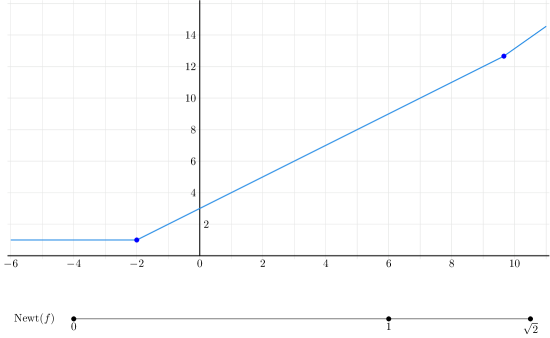
Figure 3. The graph of $f(x)=1\oplus 3\odot x\oplus-1\odot x^{\sqrt{2}}$. The connection to the Newton polytope of $f$ is explained in section 2.2.4.

2.2.3. Optimization

A tropical max-plus signomial is a piecewise-linear, continuous, convex function on $\mathbb{R}^{n}$. For a convex function, any local minimum is a global minimum. This minimum can be identified by locating the tangent plane with zero slope, which we formalize using subgradients.

Definition 2.15 ([9, §3.1.5]).

Given a convex function $f:\mathbb{R}^{n}\to\mathbb{R}$, the subdifferential of $f$ at $x$ is:

(3) $$\partial_{f}(x):=\{u\in\mathbb{R}^{n}\mid\forall z\in\mbox{dom}(f),f(z)\geq f(x)+u^{\top}\cdot(z-x)\}.$$

A subgradient of $f$ at $x$ is any element of $\partial_{f}(x)$.

The subdifferential of any function is a closed convex set. If $f$ is convex and differentiable at $x$, then the subdifferential of $f$ at $x$ is a singleton. In particular, if $f$ is linear then the subdifferential contains only the slope of $f$. And if $f$ is piecewise-linear, then $\partial_{f}(x)$ is constant on the linear pieces of $f$.

Lemma 2.16 ([9, Theorem 3.1.15]).

For any function $f$, the subdifferential at $x$ contains $\overline{\mathbf{0}}$ if and only if $x$ is a global minimizer for $f$.

Proof.

By definition, $\overline{\mathbf{0}}\in\partial_{f}(x)$ if and only if

$$\forall z\in\mbox{dom}(f),f(z)\geq f(x)+\overline{\mathbf{0}}^{\top}\cdot(z-x)\iff\forall z\in\mbox{dom}(f),f(z)\geq f(x),$$

which is if and only if $x$ is a global minimizer for $f$. ∎

Example 2.17.

Let $f(x)=1\oplus 3\odot x\oplus-1\odot x^{\sqrt{2}}$. The subdifferential of $f(x)$ on each linear piece is the slope of that piece. The subdifferential at $x=-2$ is $\partial_{f}(-2)=[0,1]$, and the subdifferential at $x=4(1+\sqrt{2})$ is $[1,\sqrt{2}]$. Note that $0$ is in the subdifferential of the constant (left-most) linear piece, and this is where the global minimum of $f(x)$ is achieved. See fig. 3.

2.2.4. Tropical Hypersurfaces

The results we stated for subgradients hold for any convex function. In this section we recall further results for tropical signomials. For a tropical polynomial $f:\mathbb{R}^{n}\to\mathbb{R}$, subdifferentials of linear pieces of $f$ are encoded by a subdivision of $\mbox{Newt}(f)$. It is this connection that will allow us to convert the problem of optimizing $f$ into a polyhedral geometry problem.

Definition 2.18.

The tropical vanishing set or tropical hypersurface of a tropical signomial $f=\bigoplus_{i}c_{i}\odot x^{\alpha_{i}}$, denoted $\mbox{tropV}(f)$, is the set of $x\in\mathbb{R}^{n}$ for which the $\max$ in $f(x)$ is achieved at least twice.

(4) $$\mbox{tropV}(f)=\{x\in\mathbb{R}^{n}\mid\max\text{ in }f(x)\text{ is achieved at least twice}\}.$$

Lemma 2.19.

The tropical vanishing set of a product of real positive powers of polynomials, $f_{i}^{w_{i}}$, is (as a set) the union of tropical vanishing sets of the $f_{i}$. That is,

$$\mbox{tropV}\left(\bigodot_{i=1}^{m}f_{i}^{w_{i}}\right)=\bigcup_{i=1}^{m}\mbox{tropV}(f_{i}),\text{ for }w_{i}>0.$$

Proof.

Let $f_{i}=\bigoplus_{\alpha\in A_{i}}c_{\alpha}\odot\mathbf{x}^{\alpha}$, $A_{i}\subset\mathbb{R}^{n}_{>0}$. If the maximum in $f_{j}$ is achieved twice by $\mathbf{x}$, then $f_{j}^{w_{j}}(\mathbf{x})=w_{j}(c_{\alpha_{1}}+\alpha_{1}\cdot\mathbf{x})=w_{j}(c_{\alpha_{2}}+\alpha_{2}\cdot\mathbf{x})$ for some $\alpha_{1}\neq\alpha_{2}\in A_{j}$. It follows that the maximum in $\bigodot_{i=1}^{m}f_{i}^{w_{i}}$ is also achieved at least twice:

$$\bigodot_{i=1}^{m}f_{i}^{w_{i}}=w_{j}(c_{\alpha_{1}}+\alpha_{1}\cdot\mathbf{x})+\sum_{i\neq j}f_{i}^{w_{i}}(\mathbf{x})=w_{j}(c_{\alpha_{2}}+\alpha_{2}\cdot\mathbf{x})+\sum_{i\neq j}f_{i}^{w_{i}}(\mathbf{x}).$$

On the other hand, if the maximum is achieved twice in $\bigodot_{i=1}^{m}f_{i}^{w_{i}}$ at $\mathbf{x}$, then we must be able to write the maximum as two distinct sums: $\sum_{i=1}^{m}w_{i}(c_{\alpha_{i}^{1}}+\alpha_{i}^{1}\cdot\mathbf{x})=\sum_{i=1}^{m}w_{i}(c_{\alpha_{i}^{2}}+\alpha_{i}^{2}\cdot\mathbf{x})$, where $\alpha_{i}^{1},\alpha_{i}^{2}\in A_{i}$. It follows that for some $j$, $\alpha_{j}^{1}\neq\alpha_{j}^{2}$, so the maximum in $f_{j}^{w_{j}}$ is achieved at least twice. ∎

A tropical hypersurface is a polyhedral complex, and it can be understood combinatorially in terms of the Newton polytope of $f$, defined below.

Definition 2.20 (Newton polytope).

Suppose $f(\mathbf{x})=\bigoplus_{\mathbf{a}\in A}c_{\mathbf{a}}\odot\mathbf{x}^{\mathbf{a}}$ is a multivariate polynomial for some finite $A\subset\mathbb{R}^{n}$ and $c_{\mathbf{a}}\in\mathbb{R}$. The support of $f(\mathbf{x})$ is the set, denoted $\mathrm{supp}(f)$, containing all $\mathbf{a}\in A$ such that $c_{\mathbf{a}}\neq-\infty$. The Newton polytope $\mathrm{Newt}(f)$ of the polynomial $f(\mathbf{x})$ is the convex hull of its support, i.e. $\mathrm{Newt}(f)=\mathrm{conv}(\mathrm{supp}(f))$. If $f,g$ are polynomials, then $\mathrm{Newt}(fg)=\mathrm{Newt}(f)+\mathrm{Newt}(g)$.

Proposition 2.21 ([8, Proposition 3.1.6]).

Given a tropical signomial $f=\sum_{i}c_{i}x^{\alpha_{i}}$, let $\underline{N}_{f}$ denote the regular subdivision of $\mbox{Newt}(f)$ induced by the weighting $w(a_{i})=c_{i}$. Then $\mbox{tropV}(f)$ is the codimension-1 skeleton of the normal complex of $\underline{N}_{f}$.

Remark 2.22.

First, although Proposition 3.1.6 in [8] is originally stated for tropical polynomials, the arguments clearly hold for tropical signomials as well. Moreover, the proof in [8] shows that the subdifferential of a linear piece of $f$ consists of the points in the corresponding cell of $\underline{N}$.

Definition 2.23.

Given a tropical polynomial $f$, let $\underline{N}$ be the regular subdivision of $\mathrm{Newt}(f)$ induced by the coefficients of $f$. The normal complex of $f$ is normal complex of $\underline{N}$; it is a subdivision of $\mathbb{R}^{n}$.

Example 2.24.

The following is an example of Proposition 2.21. Let

(5) $$f=x^{2}\oplus 4\odot xy\oplus 3\odot xz\oplus y^{2}\oplus 4\odot yz\oplus 3\odot z^{2}.$$

Figure 4 depicts $\mbox{tropV}(f)$, the subdivision of the Newton polytope dual to it, and the lift of the Newton polytope that induces that subdivision.

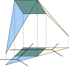
Figure 4. Left: A lift of $2\Delta^{2}=\mbox{Newt}(f)$ with weights given by the coefficients of $f$, overlaid with $\mbox{tropV}(f)$ in black; right: $\mbox{tropV}(f)$.

Lemma 2.25.

The minimum of a max-plus tropical polynomial is achieved on the cell dual to the cell of the Newton polytope containing $\overline{\mathbf{0}}$.

Proof.

Let $f=\sum_{i}c_{i}x^{\alpha_{i}}$ be a max-plus tropical polynomial (so $f$ is a piecewise-linear convex function). Let $\underline{N}$ be the regular subdivision of $\mbox{Newt}(f)$ induced by the weighting $w(\alpha_{i})=c_{i}$. Let $L$ be a linear piece of $f$, and let $N_{L}$ be the cell dual to it in $\underline{N}$. If $\overline{\mathbf{0}}\in N_{L}$, then by Proposition 2.21 $\overline{\mathbf{0}}$ is in the subdifferential of $f$ at any point in $L$. It then follows from Lemma 2.16 that the minimum of $f$ is achieved on $L$. ∎

2.3. Fermat-Weber Problems

A Fermat-Weber problem is a geometric problem seeking the median of a collection of data points $V=\{\mathbf{v}_{1},\ldots,\mathbf{v}_{m}\}\subset X$, where $X$ is a metric space with distance $d(\mathbf{x},\mathbf{y})$. We are particularly interested in the Fermat-Weber points for a collection of data points in $\mathbbm{TP}^{n-1}$, where the points could represent phylogenetic trees. The goal of this section is to introduce the Fermat-Weber problem, and reframe a tropical version as a problem on Newton polytopes.

In general, the median of a collection of points is not unique and hence we seek the set of all such medians, called the called Fermat-Weber set. The medians belonging to the Fermat-Weber set are called Fermat-Weber points. Formally, the Fermat-Weber points are the points $\mathbf{x}\in X$ minimizing the sum in (6).

Definition 2.26.

The Fermat-Weber points on the data $V=\{\mathbf{v}_{1},\ldots,\mathbf{v}_{m}\}\subset X$ are the points $\mathbf{x}\in X$ minimizing the following sum

(6) $$\mbox{FW}(V):=\frac{1}{m}\sum_{i=1}^{m}d(\mathbf{x},\mathbf{v}_{i}).$$

In this paper, we are interested in a variant of the Fermat-Weber problem, called the weighted Fermat-Weber problem. This new problem seeks the points $\mathbf{x}$ minimizing the sum in Equation 7, where the weights $w_{i}$ are positive real numbers.

(7) $$\mbox{FW}(V,\mathbf{w}):=\frac{1}{m}\sum_{i=1}^{m}w_{i}d(\mathbf{x},\mathbf{v}_{i}).$$

We will use the asymmetric tropical distance first defined by Comăneci and Joswig in [2].

Definition 2.27.

The asymmetric tropical distance, $d_{\Delta}(\mathbf{x},\mathbf{y})$ is:

(8) $$d_{\Delta}(\mathbf{x},\mathbf{y}):=n\max_{i\in[n]}(x_{i}-y_{i})+\sum_{i\in[n]}(y_{i}-x_{i}).$$

When the points $\mathbf{x},\mathbf{y}\in\mathbb{R}^{n}/\mathbb{R}\mathbbm{1}$ are given by their unique representative in $H_{0}$ (the subspace where the coordinates sum to zero), the metric $d_{\Delta}(\mathbf{x},\mathbf{y})$ can be simplified to the following

(9) $$d_{\Delta}(\mathbf{x},\mathbf{y}):=n\max_{i\in[n]}(x_{i}-y_{i}),\phantom{.}\mathbf{x},\mathbf{y}\in H_{0}.$$

Note that $d_{\Delta}(x,y)$ is invariant under independent scalar multiplication of the input vectors, so it is well-defined on $\mathbbm{TP}^{n-1}$. From now on, we will assume that all points in $\mathbbm{TP}^{n-1}$ are given by their representative in $H_{0}$. With this assumption, the distance to a point $v_{i}$ can be reinterpreted as a power of a tropical linear equations, and the sum in equation 7 can be realized as a tropical product of tropical linear functions (possibly with real exponents).

The distance to a point $v_{i}$, denote by $f_{v_{i}}(\mathbf{x})$ is

(10) $$f_{v_{i}}^{n}(\mathbf{x}):=d_{\Delta}(x,v_{i})=n\max_{j}(x_{j}-v_{ij})=\left(\bigoplus_{j=1}^{n}-v_{ij}\odot x_{j}\right)^{n}.$$

It follows that the sum in (eq. 7) for $d=d_{\Delta}$ is

(11) $$\frac{1}{m}\sum_{i=1}^{m}w_{i}d_{\Delta}(\mathbf{x},\mathbf{v}_{i})=\frac{1}{m}\sum_{i=1}^{m}w_{i}f_{v_{i}}^{nw_{i}}(\mathbf{x})=\frac{n}{m}\bigodot_{i=1}^{m}f_{v_{i}}^{w_{i}}.$$

Definition 2.28.

We define the tropical signomial associated to data $V$ with weights $\mathbf{w}$, $f_{V,\mathbf{w}}$, to be the following tropical function:

$$f_{V,\mathbf{w}}(\mathbf{x}):=\bigodot_{i=1}^{m}f_{v_{i}}^{w_{i}}=\bigodot_{i=1}^{m}\left(\bigoplus_{j=1}^{n}-v_{ij}\odot x_{j}\right)^{w_{i}}.$$

The tropical hypersurface $\mbox{tropV}(f_{v_{i}})$ is a tropical hyperplane centered at $v_{i}$; it is the codimension-1 skeleton of the normal fan of the standard simplex $\Delta^{n-1}$. By lemma 2.19, the hypersurface $\mbox{tropV}(f_{V,\mathbf{w}})$ is the union of tropical hyperplanes centered at the data points $v_{i}$. The Newton polytope of $f_{V,\mathbf{w}}=\bigodot_{i=1}^{m}f_{v_{i}}^{w_{i}}$ is $\sum_{i=1}^{m}w_{i}\cdot\Delta^{n-1}$.

Example 2.29.

The polynomial $f_{V,\mathbf{w}}(\mathbf{x})$ with $\mathbf{x}\in\mathbbm{TP}^{2}$ and $\mathbf{w}\in\mathbb{R}^{2}$ has nine terms for generic $V$ and $\mathbf{w}$.

$$f_{V,\mathbf{w}} =\left(-v_{11}\odot x_{1}\oplus-v_{12}\odot x_{2}\oplus-v_{13}\odot x_{3}\right)^{w_{1}}\odot\left(-v_{21}\odot x_{1}\oplus-v_{22}\odot x_{2}\oplus-v_{23}\odot x_{3}\right)^{w_{2}}$$

$$=(-v_{11}\odot-v_{21})\odot x_{1}^{w_{1}+w_{2}}\oplus(-v_{11}\odot-v_{22})\odot x_{1}^{w_{1}}x_{2}^{w_{2}}\oplus(-v_{11}\odot-v_{23})\odot x_{1}^{w_{1}}x_{3}^{w_{2}}$$

$$\oplus(-v_{12}\odot-v_{21})\odot x_{1}^{w_{2}}x_{2}^{w_{1}}\oplus(-v_{12}\odot-v_{22})\odot x_{2}^{w_{1}+w_{2}}\oplus(-v_{12}\odot-v_{23})\odot x_{2}^{w_{1}}x_{3}^{w_{2}}$$

$$\oplus(-v_{13}\odot-v_{21})\odot x_{1}^{w_{2}}x_{3}^{w_{1}}\oplus(-v_{13}\odot-v_{22})\odot x_{2}^{w_{2}}x_{3}^{w_{1}}\oplus(-v_{13}\odot-v_{23})\odot x_{3}^{w_{1}+w_{2}}.$$

Its Newton polytope is $(w_{1}+w_{2})\cdot\Delta^{2}$, and it is depicted in the lower right of Figure 5, with $w_{2}>w_{1}$. The image on the lower left of Figure 5 is the Newton polytope in the special case where $w_{1}=w_{2}=1$.

We now apply the results of the previous subsection to translate the problem of optimizing $f_{V,\mathbf{w}}$ into a problem on $\mbox{Newt}(f_{V,\mathbf{w}})$. Since $f_{V,\mathbf{w}}$ is a function from $\mathbbm{1}^{\perp}$ rather than $\mathbb{R}^{n}$, we need the following result to apply the results of the previous subsection.

Proposition 2.30.

Given a max-plus tropical polynomial $f:\mathbbm{1}^{\perp}\to\mathbb{R}$, let $\underline{N}$ be the subdivision of $\mathrm{Newt}(f)$ induced by the coefficients of $f$. The minimum of $f$ is achieved on the cell dual to the cell of the Newton polytope containing $\lambda\mathbbm{1}$ for any $\lambda\in\mathbb{R}\setminus\{0\}$.

Proof.

Consider the following isomorphism $\mathbb{R}^{n}/\mathbb{R}\mathbbm{1}\cong\mathbbm{1}^{\perp}$.

(12) $$\psi(x_{1},\ldots,x_{n-1})=\left(x_{1},\ldots,x_{n-1},-\sum_{i=1}^{n-1}x_{i}\right)$$

The Newton polytope of $f$ lives in $\left(\mathbbm{1}^{\perp}\right)^{\ast}$. The dual function of $\psi$ is below.

(13) $$\psi^{\ast}(x_{1},\ldots,x_{n})=\left(x_{1}-x_{n},\ldots,x_{n-1}-x_{n}\right)$$

Then $\psi^{\ast}\left(\lambda\mathbbm{1}\right)=\lambda(1-1,\ldots,1-1)=\overline{\mathbf{0}}$. Lemma 2.16 says that for a tropical function $g:\mathbb{R}^{n}\to\mathbb{R}$, the linear piece of $g$ whose dual cell contains $\overline{\textbf{0}}$ is the linear piece achieving the minimum. Combining this result with the map $\psi$, it follows that $f:\mathbbm{1}^{\perp}\to\mathbb{R}$ achieves its minimum on the linear piece dual to the cell containing $\lambda\mathbbm{1}_{n}$. ∎

2.4. Tropical Convexity

2.4.1. Tropical Factorization

Let $f=\bigodot_{i=1}^{m}f_{i}$ be a tropical signomial that factors into a product of tropical signomials. The following theorem tells us how to compute the tropical hypersurface $\mbox{tropV}(f)$ in terms of a subdivision of they Cayley polytope. Let $P_{i}=\mbox{Newt}(f_{i})$, $P=\sum_{i}P_{i}$, and write $f_{i}=\sum c_{i,\alpha}\mathbf{x}^{\alpha}$.

Theorem 2.31 (Corollary 4.9 in [6]).

Let $\underline{C}$ be the regular subdivision of $\mbox{Cayley}(P_{1},\ldots,P_{m})$ induced by the weights $w(e_{i},\alpha)=c_{i,\alpha}$. Then the mixed subdivision of $P$ corresponding to $\underline{C}$ coincides with the regular subdivsion of $P$ induced by the coefficients of $f$.

Recall that in the weighted tropical Fermat-Weber problem, $f_{V,\mathbf{w}}$ factors into linear pieces, and so theorem 2.31 applies.

Corollary 2.32.

Let $\underline{N}$ be the subdivision of $\mbox{Newt}(f_{V,\mathbf{w}})$ induced by the coefficients of $f_{V,\mathbf{w}}$. Then $\underline{N}=\underline{C}\cap\{\frac{1}{m}\mathbbm{1}_{m}\}\times\mathbb{R}^{n}$. In particular, the cell of $\underline{N}$ containing $\lambda\mathbbm{1}_{n}$ corresponds to the cell of $\underline{C}$ containing $(\frac{1}{m}\mathbbm{1}_{m},\frac{|\mathbf{w}|}{mn}\mathbbm{1}_{n})$.

Proof.

The point $(\frac{1}{m}\mathbbm{1}_{m},\frac{|\mathbf{w}|}{mn}\mathbbm{1}_{n})$ is the barycenter of $\mbox{Cayley}(P_{1},\ldots,P_{m})$, so in particular, it lies in $\mbox{Cayley}(P_{1},\ldots,P_{m})\cap\{\frac{1}{m}\mathbbm{1}_{m}\}\times\mathbb{R}^{n}$. Apply theorem 2.31 and then theorem 2.10. ∎

Proposition 2.33.

Let $P_{i}=\mbox{Newt}(f_{v_{i}})$, and let $\underline{C}^{\prime}$ be the subdivision of $\mbox{Cayley}(P_{1},\ldots,P_{m})$ induced by $w(\alpha_{j},e_{i})=-v_{ij}$. Then the subdivision of $P_{\mathbf{w}}=\sum_{i=1}^{m}w_{i}P_{i}$ induced by the coefficients of $f_{V,\mathbf{w}}$ is $\underline{C}^{\prime}\cap\{\mathbf{w}\}\times\mathbb{R}^{n}$. In particular, the cell of $\underline{P}$ containing $\mathbbm{1}_{n}$ corresponds to the cell of $\underline{C}^{\prime}$ containing $(\mathbf{w},\frac{1}{n}\mathbbm{1}_{n})$.

Proof.

Apply proposition 2.11 to corollary 2.32. ∎

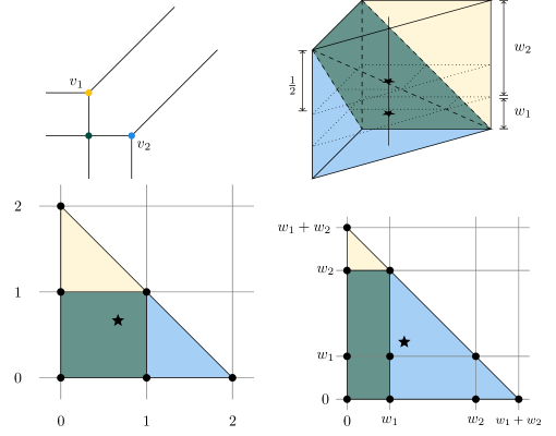
Figure 5. Subdivisions with weightings. Clockwise starting on top left: Two tropical hyperplanes in $\mathbb{TR}^{2}$, the corresponding regular subdivision of $\Delta^{1}\times\Delta^{2}$, the corresponding mixed subdivision of $(w_{1}+w_{2})\Delta^{2}$ (weighted FW problem), and the corresponding mixed subdivision of $2\Delta^{2}$ (unweighted FW problem).

2.4.2. Tropical Convex Hull

Definition 2.34.

The min-tropical convex hull of a set of points $A\subset\mathbbm{TP}^{n-1}$, denoted $\mathrm{tconv}^{\min}(A)$ or just $\mathrm{tconv}(A)$, is the set of all tropical linear combinations of points in $A$, that is,

(14) $$\mathrm{tconv}(A):=\{\lambda_{1}\odot\mathbf{a}_{1}\oplus_{\min}\cdots\oplus_{\min}\lambda_{k}\odot\mathbf{a}_{k}\mid\lambda_{i}\in\mathbb{R},\mathbf{a}_{i}\in A,k\in\mathbb{N}\}.$$

If $A$ is a finite set, then $\mathrm{tconv}(A)$ is called a tropical polytope.

Note that the tropical convex hull is independent of the representatives in $\mathbb{R}^{n}/\mathbb{R}\mathbbm{1}$ we choose for the points in $A$. That is, if $\mathbf{v}_{i}^{\prime}=\alpha_{i}\odot\mathbf{v}_{i}$, $\lambda_{i}\in\mathbb{R}$, then with $\lambda_{i}^{\prime}=\lambda_{i}-\alpha_{i}$

$$\lambda_{1}\odot v_{1}\oplus\cdots\oplus\lambda_{m}\odot v_{m}=(\lambda_{1}-\alpha_{1})\odot v_{1}^{\prime}\oplus\cdots\oplus(\lambda_{m}-\alpha_{m})\odot v_{m}=\lambda_{1}^{\prime}\odot v_{1}^{\prime}\oplus\cdots\oplus\lambda_{m}^{\prime}\odot v_{m}^{\prime}.$$

Example 2.35.

Let $v_{1}=(0,0,0)$, and $v_{2}=(1,-1,0)$. The tropical polytope $\mathrm{tconv}(v_{1},v_{2})$ consists of points of the form $\lambda_{1}\odot v_{1}\oplus\lambda_{2}\odot v_{2}$, and is illustrated in Figure 6. The tropical polytope consists of three points, connected by two classical line segments.

Figure 6. The tropical line segment between $v_{1}=(0,0,0)$ and $v_{2}=(1,-1,0)$.

It turns out that the tropical convex hull of the data points coincides with the bounded part of the tropical hypersurface $\mbox{tropV}(f_{V})$.

Theorem 2.36 (Theorem 5.2.11 in [8]).

The bounded part of the tropical hypersurface $f_{V}$ is $\mbox{tconv}^{\min}(v_{1},\ldots,v_{m})$.

We now see that $f_{V}$ and $f_{V,\mathbf{w}}$ define the same tropical hypersurface. Thus, the bounded part $\mbox{tropV}(f_{V,\mathbf{w}})$ is the tropical convex hull of the $v_{i}$’s.

Lemma 2.37.

For any $\mathbf{w}\in\mathbb{R}^{m}$, $\mbox{tropV}(f_{V})=\mbox{tropV}(f_{V,\mathbf{w}})$.

Proof.

By lemma 2.19, $\mbox{tropV}(f_{v}^{w})=\mbox{tropV}(f_{v})$ for any $v\in\mathbbm{1}^{\perp}$, and any $w>0$. Applying lemma 2.19 to $f_{V}$ and $f_{V,\mathbf{w}}$, it follows that

$$\mbox{tropV}(f_{V})=\bigcup_{i=1}^{m}\mbox{tropV}(f_{v_{i}})=\mbox{tropV}(f_{V,\mathbf{w}}).\qed$$

Corollary 2.38.

The bounded part of the tropical hypersurface $f_{V,\mathbf{w}}$ is $\mbox{tconv}^{\min}(v_{1},\ldots,v_{m})$.

3. Solving the Weighted Tropical Fermat-Weber Problem

In this section, we use combinatorics and tropical geometry to solve the weighted Fermat-Weber problem for $\mathbbm{TP}^{n-1}$ equipped with the tropical asymmetric distance. We begin by discussing the extrema of tropical polynomials.

3.1. Containment

Theorem 3.1.

Given data points $v_{1},\ldots,v_{m}\in\mathbb{R}^{n}/\mathbb{R}\mathbbm{1}$, and weights $w_{1},\ldots,w_{m}>0$, the weighted Fermat-Weber points under the tropical asymmetric metric are a cell of $\mbox{tconv}(v_{1},\ldots,v_{m})$.

Proof.

According to corollary 2.38, $\mbox{tconv}(v_{1},\ldots,v_{m})$ is the bounded part of $\mbox{tropV}(f_{V,\mathbf{w}})$. The bounded cells of $\mbox{tropV}(f_{V,\mathbf{w}})$ are exactly those cells dual to interior cells of the Newton polytope, so by proposition 2.30, it suffices to show that $\lambda\mathbbm{1}$ is in the interior of $\mbox{Newt}(f_{V,\mathbf{w}})$. The vertices of $\mbox{Newt}(f_{V,\mathbf{w}})$ are $|\mathbf{w}|e_{i}$, and their average, $\frac{|\mathbf{w}|}{n}\mathbbm{1}$, is in the interior of the Newton polytope. This proves the Fermat-Weber points are achieved on a bounded cell of $\mbox{tropV}(f_{V,\mathbf{w}})$, and therefore form a cell of $\mbox{tconv}(v_{1},\ldots,v_{m})$. ∎

3.2. Any cell can be the weighted Fermat-Weber cell

The following result shows that we can pick weights $w_{i}$ so that the weighted barycenter lies in any interior cell of the subdivision of the Cayley polytope. This finishes the proof of the main theorem.

Theorem 3.2.

Given some data points $\mathbf{v}_{1},\ldots,\mathbf{v}_{m}\in\mathbb{R}^{n}/\mathbb{R}\mathbbm{1}$, and any simplex $S$ in $\Delta^{r-1}\times\Delta^{n-1}$, which intersects the relative interior of $\Delta^{r-1}\times\Delta^{n-1}$, there is a choice of weights $w_{1},\ldots,w_{m}\in[0,1]$ with $\sum w_{i}=1$, so that $S$ contains the point $(w_{1},\ldots,w_{m},\frac{1}{n}\mathbbm{1}_{n})$.

The proof uses a well-known correspondence between subsets of the vertices of $\Delta^{m-1}\times\Delta^{n-1}$ and subgraphs of $K_{m,n}$ (the complete bipartite graph with $m$ left vertices, and $n$ right vertices), which we now briefly recall (see [3, §6.2.2] for more details). The vertex $(e_{i},e_{j})$ in a simplex $S\subseteq\Delta^{r-1}\times\Delta^{n-1}$ corresponds to the edge between left vertex $i$ and right vertex $j$ in the bipartite graph. Thus, a subset of vertices $A\subseteq\Delta^{r-1}\times\Delta^{n-1}$ corresponds to the subgraph of $K_{m,n}$.

Example 3.3 (Simplex-Forest Correspondence for $m=n=2$).

The product of two $2$-simplices (i.e. line segments) is a square; the corresponding bipartite graph has two left vertices and two right vertices. Both are illustrated in fig. 7. The vertex $(e_{i},e_{j})$ in the simplex corresponds to the edge $(l_{i},r_{j})$ in the bipartite graph. For example, the top left vertex of the shaded gray simplex, $(e_{1},e_{2})$, corresponds to the edge $(l_{1},r_{2})$. The shaded simplex is full-dimensional, so it corresponds to a spanning tree of $K_{2,2}$ (see lemma 3.4).

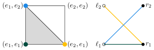
Figure 7. Vertices in the product of simplices (left) correspond to the color-coded edges of the bipartite graph (right).

Lemma 3.4 (Lemma 6.2.8 in [3]).

Let $A$ be a subset of the vertices of $\Delta^{m-1}\times\Delta^{n-1}$. Then,

1. $\mathrm{conv}(A)$ is a simplex if and only if the corresponding subgraph of $K_{m,n}$ is a forest.

2. $\mathrm{conv}(A)$ is full dimensional if and only if the corresponding subgraph of $K_{m,n}$ is spanning and connected.

Proof of Theorem 3.2.

Let $S$ be a simplex in $\Delta^{r-1}\times\Delta^{n-1}$, and let $F$ be the corresponding forest in $K_{r,n}$. Assume that $S\cap\mbox{int}\left(\Delta^{r-1}\times\Delta^{n-1}\right)\neq\emptyset$ (so $F$ is a spanning forest).

A point $(\mathbf{p},\mathbf{q})\in\mathbb{R}^{m}\times\mathbb{R}^{n}$ lies in $S$ if it can be written as a convex combination of the vertices of $S$. In terms of the forest $F$, $(\mathbf{p},\mathbf{q})$ lies in $S$ if there exist $\lambda(e)>0$ for each edge $e\in E(F)$ such that the sum of edge weights on any left vertex adds up to the corresponding $\mathbf{p}$ coordinate, and the sum of edge weights on any right vertex adds up to the corresponding $\mathbf{q}$ coordinate. Let $r(e)$ be the node on the right side connected to $e$, and let $\ell(e)$ be the node on the left side connected to $e$. The choice of $\lambda$’s in (15) leads to a valid choice of weights $w_{1},\ldots,w_{m}$ (given in (16)) so that $S$ contains the weighted barycenter.

(15) $$\lambda(e):=\frac{1}{n\cdot\deg r(e)}.$$

(16) $$w_{i}:=\sum_{e\text{ s.t. }\ell(e)=i}\lambda(e).$$

The equations in (17) show that the weights on any right node sum to $\frac{1}{n}$ (since $F$ is spanning, every vertex has at least one edge); by definition, the weights on the $i$th left node sum to $w_{i}$. It follows that $\mathbf{b}=(w_{1},\ldots,w_{m},\frac{1}{n}\mathbbm{1})$ lies in the relative interior of $S$.

(17) $$\sum_{r(e)=j}\frac{1}{n\cdot\deg(j)}=\frac{1}{n}\sum_{r(e)=j}\frac{1}{\deg(j)}=\frac{1}{n}\deg(j)\frac{1}{\deg(j)}=\frac{1}{n}.$$

Moreover, $w_{1},\ldots,w_{m}$ is a valid choice of weights for the Fermat-Weber problem. The weights $w_{i}$ are positive because $F$ is spanning, so the sum in (16) is never empty; The equations in (18) show that the $w_{i}$ sum to one.

(18) $$\sum_{i=1}^{m}w_{i}=\sum_{e}\lambda(e)=\sum_{j=1}^{n}\sum_{r(e)=j}\frac{1}{n\cdot\deg(j)}=\sum_{j=1}^{n}\frac{1}{n}\sum_{r(e)=j}\frac{1}{\deg(j)}=\sum_{j=1}^{n}\frac{1}{n}=n\frac{1}{n}=1.\qed$$

Corollary 3.5.

Given a cell $T$ in the tropical polytope $\mathrm{tconv}(\mathbf{v}_{1},\ldots,\mathbf{v}_{m})$, there is a choice of weights $w_{1},\ldots,w_{m}$ so that $T$ is the set of weighted tropical Fermat-Weber points for $\mathbf{v}_{1},\ldots,\mathbf{v}_{m}$ with weights $w_{1},\ldots,w_{m}$.

Acknowledgements

We are grateful to David Speyer and Michael Joswig for helpful conversations. This work was started at the “Algebra of phylogenetic networks” workshop held at the University of Hawai‘i at Mānoa from May 23 - 27, 2022 which was supported by the National Science Foundation under grant DMS-1945584. The first author was supported by National Science Foundation Graduate Research Fellowship under Grant No. DGE-1841052, and by the National Science Foundation under Grant No. 1855135.

References

- [1] David Bryant. A classifcation of consensus methods for phylogenetics. BioConsensus, DIMACS, 61, 05 2002.
- [2] Andrei Comăneci and Michael Joswig. Tropical medians by transportation. https://arxiv.org/abs/2205.00036, 2022.
- [3] Jesús A. De Loera, Jörg Rambau, and Francisco Santos. Triangulations, volume 25 of Algorithms and Computation in Mathematics. Springer-Verlag, Berlin, 2010. Structures for algorithms and applications.
- [4] Frank A. Fetter. Alfred weber’s theory of the location of industries. alfred weber. Journal of Political Economy, 38(2):232–234, 1930.
- [5] Birkett Huber, Jörg Rambau, and Francisco Santos. The Cayley trick, lifting subdivisions and the Bohne-Dress theorem on zonotopal tilings. J. Eur. Math. Soc. (JEMS), 2(2):179–198, 2000.
- [6] Michael Joswig. Essentials of tropical combinatorics, volume 219 of Graduate Studies in Mathematics. American Mathematical Society, Providence, RI, [2021] ©2021.
- [7] Bo Lin and Ruriko Yoshida. Tropical Fermat-Weber points. SIAM J. Discrete Math., 32(2):1229–1245, 2018.
- [8] Diane Maclagan and Bernd Sturmfels. Introduction to tropical geometry, volume 161 of Graduate Studies in Mathematics. American Mathematical Society, Providence, RI, 2015.
- [9] Yurii Nesterov. Introductory lectures on convex optimization, volume 87 of Applied Optimization. Kluwer Academic Publishers, Boston, MA, 2004. A basic course.
- [10] Francisco Santos. The Cayley trick and triangulations of products of simplices. In Integer points in polyhedra—geometry, number theory, algebra, optimization, volume 374 of Contemp. Math., pages 151–177. Amer. Math. Soc., Providence, RI, 2005.
- [11] Bernd Sturmfels. On the Newton polytope of the resultant. J. Algebraic Combin., 3(2):207–236, 1994.