Clouds and Clarity: Revisiting Atmospheric Feature Trends in Neptune-size Exoplanets

Abstract

Over the last decade, precise exoplanet transmission spectroscopy has revealed the atmospheres of dozens of exoplanets, driven largely by observatories like the Hubble Space Telescope. One major discovery has been the ubiquity of atmospheric aerosols, often blocking access to exoplanet chemical inventories. Tentative trends have been identified, showing that the clarity of planetary atmospheres may depend on equilibrium temperature. Previous work has often grouped dissimilar planets together in order to increase the statistical power of any trends, but it remains unclear from observed transmission spectra whether these planets exhibit the same atmospheric physics and chemistry. We present a re-analysis of a smaller, more physically similar sample of 15 exo-Neptune transmission spectra across a wide range of temperatures (200-1000 K). Using condensation cloud and hydrocarbon haze models, we find that the exo-Neptune population is best described by low cloud sedimentation efficiency ($\mathrm{f_{sed}}\sim 0.1$) and high metallicity ($100\times$ Solar). There is an intrinsic scatter of $\sim 0.5$ scale height, perhaps evidence of stochasticity in these planets’ formation processes. Observers should expect significant attenuation in transmission spectra of Neptune-size exoplanets, up to 6 scale heights for equilibrium temperatures between 500 and 800 K. With JWST’s greater wavelength sensitivity, colder ($<500$ K) planets should be high-priority targets given their clearer atmospheres, and the need to distinguish between the “super-puffs” and more typical gas-dominated planets.

1 Introduction

Detailed characterization has long been the goal of exoplanet astrophysics, but only in recent years has this truly been possible. In most cases, exoplanet detection studies have limited ability to probe conditions on these planets directly, leaving exoplanet characterization as a more targeted and expensive second-echelon effort. Characterization efforts can take different forms, but among the most successful has been the atmospheric characterization of gaseous exoplanets, through transmission, emission, or direct spectroscopy. Currently, direct spectroscopy requires sufficiently high-contrast imaging of widely separated, self-luminous exoplanets, while transmission and emission spectroscopy require these planets to transit their host stars, but also require sufficiently warm and large planets to produce detectable atmospheric absorption or planet-star contrast. Given current observational capabilities, transmission spectroscopy has been one of the standout successes in atmospheric characterization, driven primarily by ground-based high-resolution spectrographs as well as space-based observatories like the workhorse Hubble Space Telescope (HST). With over 5500 exoplanets known, of which $\sim 4100$ transit (NASA Exoplanet Science Institute, 2020), we now have hundreds of planets characterized through transmission spectroscopy or spectrophotometry.

However, these successes are not without their limits. These instruments often have limited spectral ranges, necessitating the use of multiple observatories, filters, and observations to observe multiple transits of an exoplanet in order to assemble broad-band atmospheric transmission spectra, and many well-known transit spectra are markedly flat (e.g., GJ 1214 b, Kreidberg et al., 2014), either due to opaque cloud layers, atmospheric hazes, or the muting of absorption features by high atmospheric metallicity, limiting our ability to determine the content of these atmospheres. A major exception has been the use of HST/WFC3 to observe water vapor absorption in dozens of exoplanetary atmospheres. $\mathrm{H}_{2}\mathrm{O}$ has a well-known absorption feature near 1.4 $\mu$m, right in the middle of HST/WFC3’s G141 grism. In clear atmospheres, this feature can be quite prominent, allowing for the direct comparison of the cloudiness or clarity of observed exoplanet transmission spectra. Where high-altitude clouds or hazes are present, observed spectra show either no water absorption or muted features, while clear atmospheres show strong water absorption.

Previous work (Stevenson, 2016; Crossfield & Kreidberg, 2017; Fu et al., 2017; Gao et al., 2020; Yu et al., 2021; Dymont et al., 2022; Edwards et al., 2023; Estrela et al., 2022) has attempted to find relationships between physical exoplanetary parameters (e.g. planet equilibrium temperature, $T_{eq}$ or surface gravity $g$) and the strength of observed atmospheric features in transmission. Stevenson (2016) performed the first systematic study of this, and introduced the method of examining clarity through the WFC3 water feature amplitude $A_{H}$ (although focusing on a surface gravity-selected sample), while initial results from (Crossfield & Kreidberg, 2017) found a linear trend in $A_{H}$ for a small sample of 6 warm Neptunes ($R_{p}\in[2,6]$ R_⊕, $T_{eq}\in[500,1100]$ K), and showed that hotter planets tend to have less aerosol obscuration than cooler planets. Fu et al. (2017) found a similar positive linear trend for a larger sample which also included transmission spectra from hotter, more massive planets, and proposed a physical explanation based on cloud condensation instead of the haze formation hypothesis from Crossfield & Kreidberg (2017). Gao et al. (2020) focused on hot (800 K – 2600 K) giant exoplanets, measuring the water feature amplitude compared to model predictions, and found that all but the hottest planets in their sample must be attenuated by clouds. Higher-order polynomial trends have been a popular model for this behavior. Yu et al. (2021) fit a parabolic trend to a sample of 9 Neptune-sized planets, but were primarily conducting an analysis of haze evolution and did not elaborate on the implications of this trend. Dymont et al. (2022) examined a larger sample of 25 planets between 200 K and 1000 K, but included rocky planets as small as $1.13~{}R_{\oplus}$ (GJ 1132 b), and Jovian planets as large as $12.9~{}R_{\oplus}$ (WASP-67 b), and also found hints of the quadratic trend from Yu et al. (2021) (without fitting any models) between $T_{eq}$ and $A_{H}$, which depends entirely on K2-18 b and LHS 1140 b. Taking a Neptune-sized 16 planet subset of their full 70-planet analysis, Edwards et al. (2023) find a parabolic trend matching theoretical predictions from Kawashima et al. (2019), while Estrela et al. (2022) fit second- and fourth-order polynomials to 62 planets from 500 to 2500 K, finding two distinct populations: aerosol-free and partially cloudy/hazy planets, with minimal aerosol presence near 1500 K.

Here, we present a trend analysis of a homogeneous sample of Neptune-like exoplanets, in order to show that sample selection is important in order to identify atmospheric feature trends, especially as JWST operations continue and provide higher-quality, broader-wavelength characterization of planetary atmospheres than possible from HST alone.

2 Sample Selection

2.1 Atmospheric Motivation

Typically, observed features are characterized by atmospheric scale heights, converting from relative units (planet-to-star radius ratio or transit depth) to physical units (kilometers), where the atmospheric scale height of a planet is (Deeg & Belmonte, 2018):

$$H=\frac{k_{B}T_{eq}}{\mu g}$$ (1)

and the depth of an absorption feature at a particular wavelength, measured in numbers of scale heights, is:

$$\delta_{\lambda}=\frac{(R_{p}+nH)^{2}}{R_{s}^{2}}-\frac{R_{p}^{2}}{R_{s}^{2}}\approx\frac{2nR_{p}H}{R_{s}^{2}}$$ (2)

Here, $K_{B}$ is Boltzmann’s constant, $T_{eq}$ the equilibrium temperature of the planet, $\mu$ the atmospheric mean molecular weight, $g$ the planet’s surface gravity, $R_{p}$ the planet radius, $R_{s}$ the stellar radius, and $n$ the number of scale heights.

However, this implies that the strength of an observed absorption feature may actually differ significantly depending on the assumed atmospheric metallicity. For example, two identical planets, at $1\times$ Solar metallicity ($\mu~{}\approx~{}2.3$ amu) and $100\times$ Solar metallicity ($\mu~{}\approx~{}3.05$ amu) will have $H_{100}/H_{1}~{}\approx~{}0.75$, and so identical-depth absorption features in a $100\times$ Solar metallicity atmosphere will be “stronger”, i.e., correspond to more scale heights than a Solar metallicity atmosphere ($n_{100}\approx 1.33n_{1}$).

Since atmospheric metallicity appears to vary across the exoplanetary mass range (Welbanks et al., 2019) and is expected from the solar system and from planetary formation models (Fortney et al., 2013), we must look at physically similar planets in a relatively narrow mass range to mitigate any mass-metallicity effect in order to have any hope of comparing their observed atmospheric features and finding underlying trends. We chose 15 planets for our analysis, including those from Crossfield & Kreidberg (2017) and others which have subsequently been observed with HST WFC3. We started with a specific radius range ($\mathrm{R_{\mathrm{pl}}}\in[2,6]$ $\mathrm{R_{\oplus}}$), in order to ensure we were not including rocky super-Earths, and included a few larger planets (HAT-P-26 b, due to it’s Neptune-like mass, and Kepler 51 b and d as, despite their low masses, they have well-known extended atmospheres and relatively low equilibrium temperatures). We also restricted our sample to temperatures $<1000$ K, in order to make sure we probe thermally-consistent atmospheric physics. As such, we do not include planets like 55 Cnc e, as it is nearly 1000 K hotter than any other planet in our sample, likely rocky, with no extended atmosphere, and has been shown not to have water vapor in its atmosphere. These planets and their physical parameters are shown in Table 1.

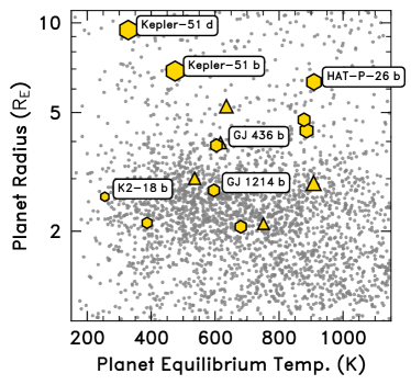
Figure 1: This work’s sample overlaid with known transiting planets. Hexagons indicate planets in our sample also being observed by JWST through Cycle 2, while triangles are not yet scheduled or approved for JWST observations. Selected targets have been labeled.

Planet (Spectrum Ref.)	Rpl	Mpl	gpl	Porb	R∗	M∗	Teff	Teq	H	$A_{H}$	Parameter Ref.
	$\mathrm{R_{\oplus}}$	$\mathrm{M_{\oplus}}$	$\mathrm{cm\,s^{-2}}$	days	$\mathrm{R_{\odot}}$	$\mathrm{M_{\odot}}$	$\mathrm{K}$	$\mathrm{K}$	$\mathrm{km}$
K2-18 b (Benneke et al., 2019a)	2.61	8.63	1241	32.9400	0.44	0.50	3457	253	56	$3.23_{-0.88}^{+0.98}$	Benneke et al. (2019a)
Kepler-51 d (Libby-Roberts et al., 2020)	9.46	5.7	62	130.1845	0.88	0.98	5670	332	1450	$0.13_{-0.08}^{+0.24}$	Libby-Roberts et al. (2020)
TOI-270 d (Mikal-Evans et al., 2023)	2.13	4.78	1029	11.3796	0.38	0.39	3506	354	94	$3.50_{-0.91}^{+1.06}$	Van Eylen et al. (2021)
Kepler-51 b (Libby-Roberts et al., 2020)	6.89	3.69	76	45.1542	0.88	0.98	5670	472	1691	$0.34_{-0.25}^{+0.41}$	Libby-Roberts et al. (2020)
HD 3167 c (Mikal-Evans et al., 2021)	3.01	9.8	1059	29.8454	0.86	0.86	5261	508	131	$1.76_{-0.89}^{+0.90}$	Christiansen et al. (2017)
GJ 1214 b (Kreidberg et al., 2014)	2.74	8.17	1064	1.5804	0.21	0.18	3250	536	137	$0.09_{-0.03}^{+0.07}$	Cloutier et al. (2021)
GJ 3470 b (Benneke et al., 2019b)	3.88	13.73	893	3.3366	0.48	0.51	3652	597	182	$1.03_{-0.26}^{+0.20}$	Biddle et al. (2014)
GJ 436 b (Knutson et al., 2014)	3.96	21.7	1355	2.6439	0.44	0.45	3585	619	125	$0.58_{-0.39}^{+0.32}$	Knutson et al. (2011)
GJ 9827 d (Roy et al., 2023)	2.07	5.2	1189	6.2015	0.61	0.61	4269	621	142	$3.21_{-1.05}^{+0.99}$	Rodriguez et al. (2018)
TOI-674 b (Brande et al., 2022)	5.25	23.6	838	1.9771	0.42	0.42	3514	661	215	$1.05_{-0.41}^{+0.46}$	Murgas et al. (2021)
HD 97658 b (Guo et al., 2020)	2.12	8.3	1809	9.4897	0.73	0.85	5212	681	103	$0.06_{-0.05}^{+0.74}$	Ellis et al. (2021)
HAT-P-11 b (Fraine et al., 2014)	4.73	25.74	1133	4.8878	0.75	0.81	4780	796	193	$2.69_{-0.64}^{+0.59}$	Bakos et al. (2010)
HD 106315 c (Kreidberg et al., 2022)	4.35	15.2	787	21.0570	1.30	1.09	6327	811	281	$1.91_{-0.87}^{+1.14}$	Barros et al. (2017)
HIP 41378 b (This Work)	2.9	8.29	965	15.5712	1.40	1.15	6199	904	255	$2.64_{-2.50}^{+2.62}$	Vanderburg et al. (2016)
HAT-P-26 b (Wakeford et al., 2017)	6.3	18.75	458	4.2345	0.79	0.82	5079	909	541	$2.97_{-0.45}^{+0.40}$	Hartman et al. (2011)

Table 1: Planets in our sample and their relevant parameters. Scale heights were calculated assuming $\mu=3.05$ amu, and equilibrium temperatures calculated assuming an albedo of 0.3.

3 Analysis

3.1 Planetary Parameters and Scale Heights

From literature values for planetary and system parameters ($R_{p}$, $M_{p}$, $P_{orb}$, $M_{*}$), we recalculated the orbital semimajor axis $a$ (according to Eq. 3), planet surface gravity $g$ (according to Eq. 4), as well as planet equilibrium temperature $T_{eq}$ (according to Eq. 5) for all planets in our sample, assuming a planetary albedo of $A=0.3$.

$$a=\left(P_{orb}^{2}\frac{GM_{*}}{4\pi^{2}}\right)^{1/3}$$ (3)

$$g=\frac{GM_{p}}{R_{p}^{2}}$$ (4)

$$T_{eq}=\mathrm{T_{eff}}\sqrt{\frac{R_{*}}{2a}}(1-A)^{1/4}$$ (5)

To calculate the scale heights of the atmospheres of these planets, we assumed $\mu=3.05$ amu (as these Neptune-sized worlds are more likely to be nearer $100\times$ Solar metallicity than $1\times$ Solar, Welbanks et al. (2019)), and calculated $H$ according to Eq. 1. Our calculated values are shown in Table 1.

3.2 Atmospheric Model Fitting and Retrievals

We used the open-source code petitRADTRANS (Mollière et al., 2019) to conduct isothermal, free-chemistry atmospheric retrievals of the archival HST/WFC3 spectra of the planets in our sample. Our retrieval framework fits for five parameters: planet mass, planet radius, isothermal atmospheric temperature, $\mathrm{H}_{2}\mathrm{O}$ abundance ($\log_{10}X$, where $X$ is the $\mathrm{H}_{2}\mathrm{O}$ mass fraction), and gray cloud deck pressure ($\log_{10}\mathrm{P}$, in bars). We placed Gaussian priors on planetary mass and radius based on the literature values and our calculated gravity distributions, a uniform prior on isothermal atmospheric temperature of $T_{eq}~{}\pm~{}200$ K, and placed uniform priors on the $\log_{10}$ cloud deck pressure (in bars, $\mathcal{U}(-6,2)$) and $\log_{10}$ water abundance (as mass fractions, $\mathcal{U}(-6,0)$) Our retrievals also included Rayleigh scattering from H₂ and He, as well as collisionally-induced-absorption of H₂-H₂ and H₂-He as continuum opacities. We fixed the reference pressure of our retrievals at 0.01 bar, and calculated model spectra at $R=1000$.

For each planet, to measure $A_{H}$, we sampled 100 random model spectra from our retrievals and rebinned them to a resolution of $R=250$, using the flux-conserving resampling method in astropy’s (Astropy Collaboration et al., 2013, 2018, 2022) specutils package. For each sampled spectrum $i$, we calculated $A_{H_{i}}~{}=~{}n_{i}~{}=~{}(\delta_{1.4,i}~{}-~{}\delta_{1.25,i})(R_{*}^{2}/2H_{i}R_{p,i})$, as re-arranged from Equation 2, where $\delta_{\lambda,i}$ is the transit depth of the sampled spectrum $i$ at wavelength $\lambda$, $R_{*}$ the stellar radius for the system in question, $R_{p,i}$ the retrieved radius of the planet for sampled spectrum $i$, $H_{i}$ the atmospheric scale height (calculated with the retrieved mass and radius values for each sampled spectrum), and $n_{i}=A_{H_{i}}$ the amplitude of the feature in numbers of scale heights $H_{i}$. The final $A_{H}$ value and its confidence interval for a particular planet was calculated from the $16^{th}$, $50^{th}$, and $84^{th}$ percentiles of the sampled values for $n_{i}$.

The observed transmission spectra and atmospheric models for our planets are shown in Figure 2.

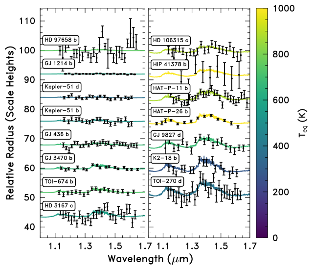
Figure 2: All HST/WFC3 G141 transmission spectra of our exo-Neptunes, scaled to show the relative $A_{H}$ values. The retrieved models are colored by the planetary equilibrium temperature, and the spectra are ordered by $A_{H}$.

3.3 Bayesian Trend Modeling

We searched for trends relating $A_{H}$ to various planetary parameters in our sample, such as equilibrium temperature, planet surface gravity, and stellar metallicity, but found no hints of useful relationships between any other than $A_{H}$ and equilibrium temperature. We then worked to identify any possible temperature dependent trend in a hierarchical Bayesian framework, in order to both distinguish between possible polynomial models as well as quantify the inherent scatter in the data. We also exclude two planets in our sample, Kepler-51 b and d, from the trend fitting, as these so-called “super-puffs” are likely not in the same physical category as the rest of the sample due to their anomalously low densities and surface gravities. It’s unclear whether these, along with GJ 1214 b and its exceptionally flat spectrum, are part of the same population as the other cold planets that have strong absorption features. Perhaps below a certain $T_{eq}$, the clarity of sub-Neptune atmospheres is essentially random with respect to $T_{eq}$, or perhaps something splits these planets into clear and cloudy populations. Studies of GJ 1214 b’s atmosphere with JWST continue to indicate it too may be unlike its peers, with especially high ($>1000\times$ Solar) metallicity (Gao et al., 2023). As such, we also exclude it from the final trend fitting.

We aim to distinguish between several trend models: one with zero correlation between $A_{H}$ and temperature ($A_{H}$ = some constant $c$), a linear model ($A_{H}$ $=~{}bt+c$) and one with a parabolic trend ($A_{H}$ $=~{}at^{2}+bt+c$), where $t$ is the equilibrium temperature. We also included an extra parameter $\sigma_{i}$ to account for unknown scatter (whether a result of stochastic astrophysical processes or various modeling insufficiencies in our polynomial trends) within our sample, added in quadrature to the measured $A_{H}$ uncertainties as $\sigma_{\mathrm{fit}}=\sqrt{\sigma_{A_{H}}^{2}+\sigma_{i}^{2}}$.

We used broad uniform priors on our model parameters, and used the No U-Turn Sampler available in exoplanet (Foreman-Mackey et al., 2021) for model fitting and posterior sampling, running 4 chains for 3000 tuning steps and 2000 draws each. After all sampler runs converged (as evidenced by the Gelman-Rubin statistic $\hat{R}$ reaching a value of 1), we calculated $\chi^{2}_{\nu}$ and BIC values for each model and found that the parabolic model

$$A_{H}=2.3\times 10^{-5}t^{2}-0.028t+9.5$$

was preferred to either the constant or linear models, with $\chi_{\nu}^{2}=2.0$ and BIC=$25.1$. The best-fit parabolic model also includes 0.56 scale height of added scatter. Our priors, fitted parameters, and model comparisons are shown in Table 2. Including the Kepler-51 planets and GJ 1214 b results in a worse fit to the data, with $\chi^{2}_{\nu}=23$ and BIC=287, as well as increases the added scatter to 0.95 scale height.

Model	Parameter	Prior	Fitted Value
Constant, $\chi^{2}_{\nu}=5.9$, BIC$=67.9$
	$c$	$\mathcal{U}(-50,50)$	$1.8^{+0.29}_{-0.27}$
	$\sigma_{i}$	$\mathcal{U}(0,10)$	$1.1^{+0.24}_{-0.20}$
Linear, $\chi^{2}_{\nu}=6.8$, BIC$=73.5$
	$b$	$\mathcal{U}(-50,50)$	$-7.1^{+15}_{-15}\times 10^{-3}$
	$c$	$\mathcal{U}(-50,50)$	$2.3^{+1.0}_{-1.0}$
	$\sigma_{i}$	$\mathcal{U}(0,10)$	$1.1^{+0.25}_{-0.20}$
Parabola, $\chi^{2}_{\nu}=2.0$, BIC$=25.1$
	$a$	$\mathcal{U}(-50,50)$	$2.3^{+0.45}_{-0.47}\times 10^{-5}$
	$b$	$\mathcal{U}(-50,50)$	$-0.028^{+0.0058}_{-0.0055}$
	$c$	$\mathcal{U}(-50,50)$	$9.5^{+1.7}_{-1.8}$
	$\sigma_{i}$	$\mathcal{U}(0,10)$	$0.56^{+0.20}_{-0.15}$

Table 2: Bayesian model fitting priors, fitted parameters, and model comparisons.

4 Model Comparisons

After identifying the best-fit parabolic trend, we compared our findings to a grid of sub-Neptune atmospheric models from Morley et al. (2015). This grid modeled the atmosphere of GJ 1214 b in clear, cloudy, and hazy configurations, across various metallicities (from $50\times$ to $1000\times$ Solar) and cloud/haze parameters. The grid was also calculated at varying insolations (compared to GJ 1214 b’s actual insolation), corresponding to $\sim 450$ K at the low end to 1100 K on the high end. As with our retrievals, we resampled the model spectra to $R=250$, and calculated $A_{H}$ using the same GJ 1214 b planetary parameters (but recalculating $H$ according to the model $T_{eq}$). The equilibrium cloud models include salt and sulfide species (ZnS, KCl, and Na₂S) calculated at varying f_sed and metallicity, and are more fully described in Section 2.3 of Morley et al. (2015). The haze models were all calculated at $50\times$ Solar metallicity, included soots with five precursor species (C₂H₂, C₂H₄, C₂H₆, C₄H₂, and HCN), calculated at varying particle sizes and precursor conversion fractions, and are more fully described in Section 2.4 of Morley et al. (2015). Using the $100\times$ and $300\times$ Solar cloudy models and the 1% and 10% haze precursor conversion fractions to bracket reasonable parameter ranges for our sample, we clearly see in Figure 3 that almost all of our sample planet spectra strongly attenuated by atmospheric aerosols compared to the clear atmosphere models.

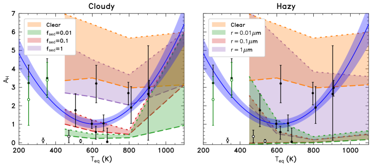
Figure 3: Retrieved spectral feature amplitude, $A_{H}$, compared to clear, cloudy, and hazy atmosphere models from Morley et al. (2015). For the clear and cloudy models, the dotted lines indicate a $100\times$ Solar metallicity atmosphere, and the dashed lines a $300\times$ Solar atmosphere. All hazy models were calculated at $50\times$ Solar metallicity, the dotted lines are 1% haze precursor conversion, and the dashed lines are 10%. The green open markers, shown for context, are the measured $\mathrm{CH}_{4}$-retrieved $A_{H}$ values for K2-18 b and TOI-270 d. The black open markers, shown for context, are the Kepler-51 planets and GJ 1214 b, which are excluded from the trend analysis.

5 Results

We calculate $\chi^{2}_{\nu}$ values for our planets with $T_{eq}~{}>~{}450$ K compared to the various contours for our clear, cloudy, and hazy models to find which set of models is most consistent with our observed $A_{H}$ values. These model comparisons are shown in Table 3. We find that all our planets are likely to be attenuated by atmospheric aerosols (sometimes very significantly, up to $\sim 6$ scale heights). This attenuation is strongest between $\sim 500$ and $\sim 700$ K, corresponding to a range of especially efficient aerosol production identified by theoretical models (Morley et al., 2015; Gao et al., 2020). The attenuation is also stronger for the $100\times$ Solar models compared to the $300\times$ Solar models.

Even so, we note some interesting points. First, with respect to the cloudy models, the majority of our planets have low sedimentation efficiency, f${}_{\mathrm{sed}}=0.1$ or lower, and the entire sample is most consistent with $\mathrm{f_{sed}}=0.01$ and $100\times$ Solar metallicity. With respect to the hazy models, our sample is most consistent with small haze particles ($r=0.01\mu$m) and small (1%) precursor conversion rates. Overall, the cloudy models fit better than the hazy models, although the sparsity of the grid means this is a relatively low-significance finding. More detailed modeling efforts may clarify this, as discussed in Section 6.

Model	$\chi^{2}_{\nu}$
Clear Models
$100\times$ Solar	149
$300\times$ Solar	32
Cloudy Models
$\mathrm{f_{sed}}=1,~{}100\times$ Solar	62
$\mathrm{f_{sed}}=1,~{}300\times$ Solar	13
$\mathrm{f_{sed}}=0.1,~{}100\times$ Solar	2.9
$\mathrm{f_{sed}}=0.1,~{}300\times$ Solar	4.7
$\mathrm{f_{sed}}=0.01,~{}100\times$ Solar	3.8
$\mathrm{f_{sed}}=0.01,~{}300\times$ Solar	9.0
Hazy Models
$\mathrm{r}=1\mu$m, 1% conversion	102
$\mathrm{r}=1\mu$m, 10% conversion	8.6
$\mathrm{r}=0.1\mu$m, 1% conversion	8.1
$\mathrm{r}=0.1\mu$m, 10% conversion	12.6
$\mathrm{r}=0.01\mu$m, 1% conversion	7.4
$\mathrm{r}=0.01\mu$m, 10% conversion	12.9

Table 3: Atmospheric models and model comparisons.

Second, while they were not included in the trend fitting, the Kepler-51 planets cannot be totally ignored. While these “super-puffs” clearly stand out as exceptionally low-density planets, other temperate, puffy sub-Neptunes have been discovered since (e.g. TOI-700 c, WASP-193 b), which will also be amenable to atmospheric transmission spectroscopy. Observing as many cold planets as possible is sorely needed to determine whether our observed trend holds. These observations would identify whether cold sub-Neptunes exist in a continuum between the slightly attenuated atmospheres which follow our trend and the especially cloudy and hazy planets like the Kepler-51 planets and GJ 1214 b. If these are outliers among the broader population, it bodes well for future studies of habitable zone systems. Perhaps there is a range of temperatures where cloud rainout is efficient (especially for heavier species like ZnS and KCl) while low insolation means haze production is not, giving especially clear views into these temperate planets’ atmospheres.

Finally, we find that, among our sample of Neptune-sized exoplanets, there is an intrinsic scatter in the clarity of these atmospheres of $\sim 0.5$ scale height. This scatter may be evidence that our trend model choices are insufficient, or possibly be due to some randomness in the outcomes of planet formation and evolutionary processes. Perhaps the trend identified is analogous to a “main sequence” of planetary atmospheres, and (taking into account the super-puffs) future observations with JWST will be able to confirm or reject our identification of this scatter.

We also note that, while we used water vapor as the major opacity source in this analysis, methane absorption has significant overlap with water in near-IR bands, and may dominate compared to water vapor in certain exoplanetary atmospheres $<600$ K (Bézard et al., 2022). In fact, this has been identified in K2-18 b, previously thought to have water vapor in its atmosphere from HST data (Benneke et al., 2019a), but now shown instead to have methane from broad-wavelength JWST observations (Madhusudhan et al., 2023). With this in mind, we also ran methane-only retrievals for K2-18 b and TOI-270 d to compare to our water-only retrievals and found the methane-calculated $A_{H}$ values to be consistent within the $1\sigma$ uncertainties. The substitution of $\mathrm{CH}_{4}$ for $\mathrm{H}_{2}\mathrm{O}$ in these coolest planets does not change our conclusions. These are shown in Figure 3 as open green markers.

These results echo previous analyses: our model comparisons provide evidence for a cloud-based mechanism shaping this trend (predicted by Fu et al. (2017)) over a haze-driven trend (predicted by Crossfield & Kreidberg (2017) and Yu et al. (2021)). Qualitatively, our quadratic trend behaves similarly to previous second-order trends fit to samples that extend to low temperatures (Yu et al., 2021; Edwards et al., 2023), showing significant increases in atmospheric clarity at cold ($<500$K) and hotter ($>700$K). The major differences between these trends are primarily due to sampling, as the inclusion of particular planets (like Kepler-51 d in Yu et al. (2021) and Edwards et al. (2023)) can shift the parabola minimum to colder equilibrium temperatures. Robustness against planetary samples is encouraging, as it appears the observational predictions made by these trends will be useful for a broad range of future spectroscopic studies. Most of our measured $A_{H}$ values are also consistent to previous analyses within error, although our method differs to previous analyses due to our retrieval framework. This confirms that, as an observational metric, $A_{H}$ is robust against methodological changes (even if the physical insights gained about any particular planet transmission spectrum from $A_{H}$ alone appear to be limited).

6 Community Priorities

Despite the proliferation of HST WFC3 transmission spectra in recent years, significant trends relating the clarity of these atmospheres to planetary and system parameters still evade us. WFC3, while especially sensitive to water vapor and uniform cloud absorption within a narrow spectral range, cannot characterize the full panoply of absorbers present in exoplanet atmospheres (perhaps most significantly shown by K2-18 b’s JWST methane detection in Madhusudhan et al. (2023) over the HST water detection from (Benneke et al., 2019a)), nor precisely constrain physical cloud models. As already shown from the first year of JWST analyses, exoplanetary atmospheres are complex, dynamic, and contain clear evidence of atmospheric physics beyond anything HST could provide (JWST Transiting Exoplanet Community Early Release Science Team et al., 2023; Rustamkulov et al., 2023; Alderson et al., 2023; Feinstein et al., 2023; Ahrer et al., 2023; Tsai et al., 2023).

Among the scheduled and completed JWST programs (through Cycle 2), there are 106 unique exoplanet systems. Of the planets in these systems, 36 fit our sample radius criteria ($\mathrm{R_{\mathrm{pl}}}\in[2,6]$ $\mathrm{R_{\oplus}}$). 8 of the planets we analyzed in this work are on this list as well, although these alone are not sufficient to adequately sample the range of equilibrium temperatures. We need to add more exoplanets to the JWST observational sample, especially temperate planets that are large enough to sustain extended atmospheres, so we can confirm the $<500$K leg of the trend observed in this work.

We also need significantly improved model grids for sub-Neptune atmospheres. Aerosol production is a complex process, and low-resolution observations have historically been unable to reveal much about these. New JWST observations, with higher resolution and much broader wavelength range, have already identified signatures of wavelength-dependent silicate cloud absorption in the planetary-mass object VHS 1256 b (Miles et al., 2023). Haze precursors like SO₂ have been identified in the Hot Jupiter WASP-39 b (Rustamkulov et al., 2023; Alderson et al., 2023; Tsai et al., 2023), and GJ 1214 b’s high-altitude aerosols have been found to be very reflective ($A=0.51$, Kempton et al., 2023). Extending modeling efforts to colder planets, across a wide range of metallicities, cloud species, particle sizes, atmospheric mixing, and other parameters should enable us to constrain these processes in these planets’ atmospheres.

7 Conclusions

We have identified a coherent trend relating the clarity of Neptune-sized planetary atmospheres to their equilibrium temperatures, as well as modeling the intrinsic scatter in planetary clarity measurements, across an $\sim 800$K temperature range. These findings show behavior similar to previous analyses, again finding a parabolic trend with clearer atmospheres at cooler ($<500$K) and hotter ($>700$K), with a minimum between $500-700$ K. We reproduce this behavior for our restricted sample of Neptune-like planets compared to more diverse samples in previous analyses, implying the observational implications of this work should be applicable to many future HST and JWST targets. Compared to models, all observed planetary atmospheres are consistent with attenuation by at least some cloud cover as a result of vertically extended clouds or hazes with small particles ($\mathrm{f_{sed}}=0.1$, $r=0.01\mu$m), and have relatively high metallicity ($\sim 100\times$ solar). Confirmation or rejection of cold-temperature theoretical predictions still eludes us, as we need updated self-consistent modeling efforts across a range of atmospheric parameters for these cold planets. JWST observations in the next few cycles should both continue to test our identified trend, and help identify the atmospheric diversity that may be present among cold ($T_{eq}<500$ K) planets.

Appendix A HIP 41378 b

HIP 41378 b was included as a target in HST program GO-15333, which also observed HD 3167 c, GJ 9827 d, TOI-674 b, and HD 106315 c.

We observed two transits of HIP 41378 b with HST’s WFC3 instrument, using the G141 grism, before dropping this planet in favor of TOI-674 b (Brande et al., 2022) due to scheduling difficulties. We followed standard data reduction procedures for HST/WFC3 time series data, as documented in Kreidberg et al. (2022). Following common practice, we fit the light curves simultaneously with a transit model and an instrument systematics model. Our transit model included variable $R_{p}/R_{*}$, and other system parameters were fixed to the best-fit values from (Berardo et al., 2019). The limb darkening parameters were fixed on predictions from a PHOENIX stellar model at the effective temperature of the host star. The instrument systematics model consisted of a visit-long linear slope, a scaling factor between upstream and downstream spatial scans, and exponential ramps fit to each orbit (following the model ramp parameterisation from Kreidberg et al., 2022). The observed transmission spectrum is given in Table 4. The raw data for HIP 41378 b is available at Mikulski Archive for Space Telescopes (MAST) at the Space Telescope Science Institute at the following DOI:https://doi.org/10.17909/ryg6-3c46 (catalog 10.17909/ryg6-3c46).

Wavelength	Transit Depth $(R_{p}/R_{*})^{2}$
($\mu$m)	(ppm)
1.175	$347\pm 32.7$
1.225	$273\pm 32.2$
1.275	$244\pm 35.5$
1.325	$326\pm 28.6$
1.375	$302\pm 32.7$
1.425	$285\pm 33.2$
1.475	$320\pm 34.9$
1.525	$296\pm 34.7$
1.575	$283\pm 35.6$
1.625	$294\pm 41.1$

Table 4: HIP 41378 b HST/WFC3 G141 Transmission Spectrum

References

- Ahrer et al. (2023) Ahrer, E.-M., Stevenson, K. B., Mansfield, M., et al. 2023, Nature, 614, 653, doi: 10.1038/s41586-022-05590-4
- Alderson et al. (2023) Alderson, L., Wakeford, H. R., Alam, M. K., et al. 2023, Nature, 614, 664, doi: 10.1038/s41586-022-05591-3
- Astropy Collaboration et al. (2013) Astropy Collaboration, Robitaille, T. P., Tollerud, E. J., et al. 2013, A&A, 558, A33, doi: 10.1051/0004-6361/201322068
- Astropy Collaboration et al. (2018) Astropy Collaboration, Price-Whelan, A. M., Sipőcz, B. M., et al. 2018, AJ, 156, 123, doi: 10.3847/1538-3881/aabc4f
- Astropy Collaboration et al. (2022) Astropy Collaboration, Price-Whelan, A. M., Lim, P. L., et al. 2022, ApJ, 935, 167, doi: 10.3847/1538-4357/ac7c74
- Bakos et al. (2010) Bakos, G. Á., Torres, G., Pál, A., et al. 2010, ApJ, 710, 1724, doi: 10.1088/0004-637X/710/2/1724
- Barros et al. (2017) Barros, S. C. C., Gosselin, H., Lillo-Box, J., et al. 2017, A&A, 608, A25, doi: 10.1051/0004-6361/201731276
- Benneke et al. (2019a) Benneke, B., Wong, I., Piaulet, C., et al. 2019a, ApJ, 887, L14, doi: 10.3847/2041-8213/ab59dc
- Benneke et al. (2019b) Benneke, B., Knutson, H. A., Lothringer, J., et al. 2019b, Nature Astronomy, 3, 813, doi: 10.1038/s41550-019-0800-5
- Berardo et al. (2019) Berardo, D., Crossfield, I. J. M., Werner, M., et al. 2019, AJ, 157, 185, doi: 10.3847/1538-3881/ab100c
- Bézard et al. (2022) Bézard, B., Charnay, B., & Blain, D. 2022, Nature Astronomy, 6, 537, doi: 10.1038/s41550-022-01678-z
- Biddle et al. (2014) Biddle, L. I., Pearson, K. A., Crossfield, I. J. M., et al. 2014, MNRAS, 443, 1810, doi: 10.1093/mnras/stu1199
- Brande et al. (2022) Brande, J., Crossfield, I. J. M., Kreidberg, L., et al. 2022, AJ, 164, 197, doi: 10.3847/1538-3881/ac8b7e
- Chen & Kipping (2017) Chen, J., & Kipping, D. 2017, ApJ, 834, 17, doi: 10.3847/1538-4357/834/1/17
- Christiansen et al. (2017) Christiansen, J. L., Vanderburg, A., Burt, J., et al. 2017, AJ, 154, 122, doi: 10.3847/1538-3881/aa832d
- Cloutier et al. (2021) Cloutier, R., Charbonneau, D., Deming, D., Bonfils, X., & Astudillo-Defru, N. 2021, AJ, 162, 174, doi: 10.3847/1538-3881/ac1584
- Crossfield & Kreidberg (2017) Crossfield, I. J. M., & Kreidberg, L. 2017, AJ, 154, 261, doi: 10.3847/1538-3881/aa9279
- Deeg & Belmonte (2018) Deeg, H. J., & Belmonte, J. A. 2018, Handbook of Exoplanets, doi: 10.1007/978-3-319-55333-7
- Dymont et al. (2022) Dymont, A. H., Yu, X., Ohno, K., et al. 2022, ApJ, 937, 90, doi: 10.3847/1538-4357/ac7f40
- Edwards et al. (2023) Edwards, B., Changeat, Q., Tsiaras, A., et al. 2023, ApJS, 269, 31, doi: 10.3847/1538-4365/ac9f1a
- Ellis et al. (2021) Ellis, T. G., Boyajian, T., von Braun, K., et al. 2021, AJ, 162, 118, doi: 10.3847/1538-3881/ac141a
- Estrela et al. (2022) Estrela, R., Swain, M. R., & Roudier, G. M. 2022, ApJ, 941, L5, doi: 10.3847/2041-8213/aca2aa
- Feinstein et al. (2023) Feinstein, A. D., Radica, M., Welbanks, L., et al. 2023, Nature, 614, 670, doi: 10.1038/s41586-022-05674-1
- Foreman-Mackey et al. (2021) Foreman-Mackey, D., Luger, R., Agol, E., et al. 2021, The Journal of Open Source Software, 6, 3285, doi: 10.21105/joss.03285
- Fortney et al. (2013) Fortney, J. J., Mordasini, C., Nettelmann, N., et al. 2013, ApJ, 775, 80, doi: 10.1088/0004-637X/775/1/80
- Fraine et al. (2014) Fraine, J., Deming, D., Benneke, B., et al. 2014, Nature, 513, 526, doi: 10.1038/nature13785
- Fu et al. (2017) Fu, G., Deming, D., Knutson, H., et al. 2017, ApJ, 847, L22, doi: 10.3847/2041-8213/aa8e40
- Gao et al. (2020) Gao, P., Thorngren, D. P., Lee, E. K. H., et al. 2020, Nature Astronomy, 4, 951, doi: 10.1038/s41550-020-1114-3
- Gao et al. (2023) Gao, P., Piette, A. A. A., Steinrueck, M. E., et al. 2023, ApJ, 951, 96, doi: 10.3847/1538-4357/acd16f
- Guo et al. (2020) Guo, X., Crossfield, I. J. M., Dragomir, D., et al. 2020, AJ, 159, 239, doi: 10.3847/1538-3881/ab8815
- Hartman et al. (2011) Hartman, J. D., Bakos, G. Á., Kipping, D. M., et al. 2011, ApJ, 728, 138, doi: 10.1088/0004-637X/728/2/138
- JWST Transiting Exoplanet Community Early Release Science Team et al. (2023) JWST Transiting Exoplanet Community Early Release Science Team, Ahrer, E.-M., Alderson, L., et al. 2023, Nature, 614, 649, doi: 10.1038/s41586-022-05269-w
- Kawashima et al. (2019) Kawashima, Y., Hu, R., & Ikoma, M. 2019, ApJ, 876, L5, doi: 10.3847/2041-8213/ab16f6
- Kempton et al. (2023) Kempton, E. M. R., Zhang, M., Bean, J. L., et al. 2023, Nature, 620, 67, doi: 10.1038/s41586-023-06159-5
- Knutson et al. (2014) Knutson, H. A., Benneke, B., Deming, D., & Homeier, D. 2014, Nature, 505, 66, doi: 10.1038/nature12887
- Knutson et al. (2011) Knutson, H. A., Madhusudhan, N., Cowan, N. B., et al. 2011, ApJ, 735, 27, doi: 10.1088/0004-637X/735/1/27
- Kreidberg et al. (2014) Kreidberg, L., Bean, J. L., Désert, J.-M., et al. 2014, Nature, 505, 69, doi: 10.1038/nature12888
- Kreidberg et al. (2022) Kreidberg, L., Mollière, P., Crossfield, I. J. M., et al. 2022, AJ, 164, 124, doi: 10.3847/1538-3881/ac85be
- Libby-Roberts et al. (2020) Libby-Roberts, J. E., Berta-Thompson, Z. K., Désert, J.-M., et al. 2020, AJ, 159, 57, doi: 10.3847/1538-3881/ab5d36
- Madhusudhan et al. (2023) Madhusudhan, N., Sarkar, S., Constantinou, S., et al. 2023, arXiv e-prints, arXiv:2309.05566, doi: 10.48550/arXiv.2309.05566
- Mikal-Evans et al. (2021) Mikal-Evans, T., Crossfield, I. J. M., Benneke, B., et al. 2021, AJ, 161, 18, doi: 10.3847/1538-3881/abc874
- Mikal-Evans et al. (2023) Mikal-Evans, T., Madhusudhan, N., Dittmann, J., et al. 2023, AJ, 165, 84, doi: 10.3847/1538-3881/aca90b
- Miles et al. (2023) Miles, B. E., Biller, B. A., Patapis, P., et al. 2023, ApJ, 946, L6, doi: 10.3847/2041-8213/acb04a
- Mollière et al. (2019) Mollière, P., Wardenier, J. P., van Boekel, R., et al. 2019, A&A, 627, A67, doi: 10.1051/0004-6361/201935470
- Morley et al. (2015) Morley, C. V., Fortney, J. J., Marley, M. S., et al. 2015, ApJ, 815, 110, doi: 10.1088/0004-637X/815/2/110
- Murgas et al. (2021) Murgas, F., Astudillo-Defru, N., Bonfils, X., et al. 2021, A&A, 653, A60, doi: 10.1051/0004-6361/202140718
- NASA Exoplanet Science Institute (2020) NASA Exoplanet Science Institute. 2020, Planetary Systems Table, IPAC, doi: 10.26133/NEA12
- Rodriguez et al. (2018) Rodriguez, J. E., Vanderburg, A., Eastman, J. D., et al. 2018, AJ, 155, 72, doi: 10.3847/1538-3881/aaa292
- Roy et al. (2023) Roy, P.-A., Benneke, B., Piaulet, C., et al. 2023, ApJ, 954, L52, doi: 10.3847/2041-8213/acebf0
- Rustamkulov et al. (2023) Rustamkulov, Z., Sing, D. K., Mukherjee, S., et al. 2023, Nature, 614, 659, doi: 10.1038/s41586-022-05677-y
- Stevenson (2016) Stevenson, K. B. 2016, ApJ, 817, L16, doi: 10.3847/2041-8205/817/2/L16
- Tsai et al. (2023) Tsai, S.-M., Lee, E. K. H., Powell, D., et al. 2023, Nature, 617, 483, doi: 10.1038/s41586-023-05902-2
- Van Eylen et al. (2021) Van Eylen, V., Astudillo-Defru, N., Bonfils, X., et al. 2021, MNRAS, 507, 2154, doi: 10.1093/mnras/stab2143
- Vanderburg et al. (2016) Vanderburg, A., Becker, J. C., Kristiansen, M. H., et al. 2016, ApJ, 827, L10, doi: 10.3847/2041-8205/827/1/L10
- Wakeford et al. (2017) Wakeford, H. R., Sing, D. K., Kataria, T., et al. 2017, Science, 356, 628, doi: 10.1126/science.aah4668
- Welbanks et al. (2019) Welbanks, L., Madhusudhan, N., Allard, N. F., et al. 2019, ApJ, 887, L20, doi: 10.3847/2041-8213/ab5a89
- Yu et al. (2021) Yu, X., He, C., Zhang, X., et al. 2021, Nature Astronomy, 5, 822, doi: 10.1038/s41550-021-01375-3