Abstract

The Seiberg-Witten solution to four-dimensional ${\cal N}=2$ super-Yang-Mills theory with gauge group ${\text{SU}}(N)$ and without hypermultiplets is used to investigate the neighborhood of the maximal Argyres-Douglas points of type $(\mathfrak{a}_{1},\mathfrak{a}_{N-1})$. A convergent series expansion for the Seiberg-Witten periods near the Argyres-Douglas points is obtained by analytic continuation of the series expansion around the ${\mathbb{Z}}_{2N}$ symmetric point derived in arXiv:2208.11502. Along with direct integration of the Picard-Fuchs equations for the periods, the expansion is used to determine the location of the walls of marginal stability for ${\text{SU}}(3)$. The intrinsic periods and Kähler potential of the $(\mathfrak{a}_{1},\mathfrak{a}_{N-1})$ superconformal fixed point are computed by letting the strong coupling scale tend to infinity. We conjecture that the resulting intrinsic Kähler potential is positive definite and convex, with a unique minimum at the Argyres-Douglas point, provided only intrinsic Coulomb branch operators with unitary scaling dimensions $\Delta>1$ acquire a vacuum expectation value, and provide both analytical and numerical evidence in support of this conjecture. In all the low rank examples considered here, it is found that turning on moduli dual to $\Delta\leq 1$ operators spoils the positivity and convexity of the intrinsic Kähler potential.

1 Introduction

The Seiberg-Witten (SW) solution to four dimensional ${\cal N}=2$ super-Yang-Mills theory provides the exact low energy effective action and BPS mass spectrum on the Coulomb branch. The vacuum expectation values (VEVs) of the gauge scalars and their magnetic duals are encoded in terms of a family of Riemann surfaces equipped with a meromorphic differential, referred to as the SW curve and the SW differential, respectively. The original construction was given for gauge group ${\text{SU}}(2)$ in [1, 2]. In the present paper, we focus on theories with gauge group ${\text{SU}}(N)$, primarily for $N\geq 3$ and without hypermultiplets, for which the SW curve and differential were constructed in [3, 4, 5, 6] (see also [8, 7, 9, 10, 11]).

At generic points on the Coulomb branch, the gauge group ${\text{SU}}(N)$ is spontaneously broken to its maximal Abelian subgroup ${\text{U}}(1)^{N-1}$ and the low energy contents of the theory consist of $N-1$ massless Abelian ${\cal N}=2$ gauge multiplets. The spectrum of massive BPS states includes the $N(N-1)$ gauge bosons and their magnetic counterparts. Remarkably, the SW solution predicts the existence of isolated points in the moduli space where the masses of one or several of these BPS state tends to zero. We now describe two distinct scenarios where a maximal number of massive BPS states become simultaneously massless.

There are $N$ multi-monopole points in the moduli space, at each one of which $N-1$ mutually local (i.e. with vanishing Dirac pairing) BPS states become simultaneously massless. At each multi-monopole point, there exists an ${\text{Sp}}(2N-2,{\mathbb{Z}})$ electric-magnetic duality frame in which all the massless BPS states have purely magnetic charges, whence the name. In view of their mutual locality, there exists an effective field theory description where the massless magnetic monopoles are described by hypermultiplets. Investigations into the behavior of the effective prepotential and periods in the neighborhood of a multi-monopole point may be found in [12, 13, 14] as well as in [15], where the behavior of the Kähler potential and the walls of marginal stability are analyzed.

For gauge group ${\text{SU}}(3)$, Argyres and Douglas discovered two so-called AD points in the moduli space, where three mutually non-local BPS states (i.e. with non-vanishing Dirac pairing) simultaneously become massless [16]. The corresponding AD theories are strongly interacting ${\cal N}=2$ superconformal field theories (SCFTs). For gauge group ${\text{SU}}(N)$ with $N>3$ the maximal number of mutually non-local BPS states become massless at two maximal AD points, thereby generalizing the case of $N=3$, while, for $N=2$, no AD points exist. Since the Dirac pairing is invariant under ${\text{Sp}}(2N-2,{\mathbb{Z}})$, there is no electric-magnetic duality frame in which the massless BPS states are mutually local and simultaneously admit a standard local field theory description.

While the absence of a standard local field theory formulation of the AD theories presents a considerable conceptual challenge, several indirect avenues of investigation have been explored, including the superconformal bootstrap and brane constructions in string theory. Here, we shall investigate the space of theories in the vicinity of the maximal AD points, first by exploring the Coulomb branch of their embedding in ${\text{SU}}(N)$ super-Yang-Mills and second by exploring their intrinsic Coulomb branch obtained by sending the strong coupling scale $\Lambda$ of the ${\text{SU}}(N)$ theory to infinity. The organization of the remainder of the paper and an overview of the results is presented in the subsections below.

  $\bullet$ Series expansion near the maximal Argyres-Douglas points

In section 2, we compute the SW periods in a convergent series expansion around the maximal AD points. Our expansion provides a non-trivial analytic continuation of the strong-coupling expansion produced in [15] around the unique ${\mathbb{Z}}_{2N}$-symmetric point. While the latter expansion contains the AD and the multi-monopole points on the boundary of its domain of convergence, our expansion is centered at one or the other AD point and thereby provides a significant extension of the domain of convergence near the AD points. On regions where they overlap, our expansion arguably has better convergence properties than the one given in [15]. Finally, by taking the decoupling limit $\Lambda\rightarrow\infty$, where $\Lambda$ is the strong-coupling scale, we obtain the intrinsic AD periods for $(\mathfrak{a}_{1},\mathfrak{a}_{N-1})$ superconformal field theories in section 4.

  $\bullet$ Charting candidate walls of marginal stability

Two BPS states with central charges $Z_{1}$ and $Z_{2}$ and masses $M_{1}=|Z_{1}|$ and $M_{2}=|Z_{2}|$ can form a stable bound state provided its mass $M$ obeys $M<M_{1}+M_{2}$. The bound state is BPS when $M=|Z_{1}+Z_{2}|$, and becomes marginally stable when the binding energy vanishes, namely when $|Z_{1}+Z_{2}|=|Z_{1}|+|Z_{2}|$, which requires the ratio $Z_{2}/Z_{1}$ bo be a real number. The reality of $Z_{2}/Z_{1}$ defines a real co-dimension one sub-variety of the Coulomb branch, referred to as a candidate wall of marginal stability. Determining this sub-variety was already undertaken in [1, 2] for gauge group ${\text{SU}}(2)$, and discussed in more detail in [17, 18, 19]. Candidate walls of marginal stability were investigated more recently in [15] for gauge group ${\text{SU}}(N)$ on restricted slices through the Coulomb branch.

In section 3, we shall map out candidate walls of marginal stability beyond the restricted slices of [15] for gauge group ${\text{SU}}(3)$, and present partial results for $N\geq 4$. The series expansion around the AD points, discussed in the preceding subsection, will play a key role in gaining access to the walls of marginal stability beyond the special slices studied in [15]. In addition, we shall adapt the numerical integration methods used in [15] to the computation of the SW periods and the central charges. These numerical computations will allow us to reach beyond the radius of convergence of either the ${\mathbb{Z}}_{2N}$ or the AD expansion, and to complete the charting of candidate walls of marginal stability.

  $\bullet$ Exploring the intrinsic Kähler potential of the $(\mathfrak{a}_{1},\mathfrak{a}_{N-1})$ AD theories

Interest in the behavior of the Kähler potential, within the context of the SW solution, has recently been rekindled by the role it may play in the soft breaking of ${\cal N}=2$ super Yang-Mills theory and the renormalization group flow of this theory to adjoint QCD [20, 14, 15, 21]. Specifically, the flow of the mass operator $M^{2}{\rm tr}(\phi^{\dagger}\phi)$ for the gauge scalar $\phi$ purely within the ${\cal N}=2$ super Yang-Mills theory is to the Kähler potential of the SW solution. Motivated in part by future work on soft supersymmetry breaking in or near AD theories, we initiate here a study of the intrinsic Kähler potential of the maximal AD theories. Key questions concern its positivity, convexity, and global minima properties.

In section 4, we shall study the intrinsic periods of the AD theories; calculate the intrinsic Kähler potential; investigate the location of its minima; and understand its positivity and convexity properties. We will find that, in the absence of deformations, namely moduli corresponding to operators with dimension $\Delta\leq 1$, but allowing the VEVs of genuine Coulomb branch operators with dimension $\Delta>1$ to be non-zero, the intrinsic Kähler potential exhibits positivity and convexity. This distinction between the dimensions coincides precisely with the unitarity bound on scaling dimensions of operators in any ${\cal N}=2$ SCFT: $\Delta\geq 1$, where free bosonic fields saturate this bound. We shall gather compelling evidence that turning on Coulomb branch operators with unitary scaling dimensions is compatible with maintaining positivity and convexity of the Kähler potential, and its unique global minimum being at the AD point.

Acknowledgements

We gratefully acknowledge useful conversations with Thomas Dumitrescu and Emily Nardoni. SB is happy to thank Lukas Lindwasser for conceptual discussions and Amey Gaikwad for suggestions on numerical calculations. This research was supported in part by the National Science Foundation under grant PHY-22-09700.

2 Series expansion near a maximal AD point

We begin this section with a brief summary of the salient features of the Seiberg-Witten (SW) solution for four-dimensional ${\cal N}=2$ super Yang-Mills theory gauge group ${\text{SU}}(N)$ without hyper-multiplets [3, 4, 7]. We also review the expansion of the SW solution around the ${\mathbb{Z}}_{2N}$ symmetric point obtained in [15]. A similar set-up is then used to derive a convergent expansion of the SW periods near one of the ${\mathbb{Z}}_{N}$ symmetric maximal AD points for $N\geq 3$, and to show that this expansion coincides with the analytic continuation of the ${\mathbb{Z}}_{2N}$ expansion of [15]. A key tool in matching the expansions is the Gauss-Kummer quadratic transformation on hypergeometric functions. A detailed analysis of the domain of convergence is undertaken and its results are presented graphically.

2.1 Summary of the Seiberg-Witten solution

The SW solution determines the vacuum expectation values of the gauge scalars $a_{I}(u)$ and their magnetic duals $a_{D,I}(u)$ as locally holomorphic functions of the gauge invariant Coulomb branch moduli $u_{n}$ for $I=1,\cdots,N-1$ and $n=0,1,\ldots,N-2$. The SW solution is constructed from a family of Riemann surfaces ${\cal C}(u)$ that depends holomorphically on the moduli $u_{n}$ and is referred to as the Seiberg-Witten curve. For gauge group ${\text{SU}}(N)$ and no hyper-multiplets, the SW curve is given by,

$$y^{2}=A(x)^{2}-\Lambda^{2N}\,,\hskip 57.81621ptA(x)=x^{N}-\sum_{n=0}^{N-2}u_{n}x^{n}\,,$$ (2.1)

where $\Lambda$ is the strong-coupling scale of the non-Abelian ${\text{SU}}(N)$ super Yang-Mills theory. Each Riemann surface in the family is hyper-elliptic and has genus $N-1$. Choosing a basis of homology cycles $\mathfrak{A}_{I}$ and $\mathfrak{B}_{I}$ with canonical intersection pairing $\mathfrak{J}$,

$$\mathfrak{J}(\mathfrak{A}_{I},\mathfrak{B}_{J})=-\mathfrak{J}(\mathfrak{B}_{I},\mathfrak{A}_{J}) = \delta_{IJ}$$

$$\mathfrak{J}(\mathfrak{A}_{I},\mathfrak{A}_{J})\,=\,\mathfrak{J}(\mathfrak{B}_{I},\mathfrak{B}_{J}) = 0~{},$$ (2.2)

the vacuum expectation values of the gauge scalars $a_{I}(u)$ and their magnetic duals $a_{D,I}(u)$ are obtained as the periods of a meromorphic Abelian differential $\lambda$ as follows,

$$2\pi i\,a_{I}=\oint_{\mathfrak{A}_{I}}\lambda\,,\hskip 65.76596pt2\pi i\,a_{D,I}=\oint_{\mathfrak{B}_{I}}\lambda\,\hskip 65.76596pt\lambda={xA^{\prime}(x)dx\over y}\,.$$ (2.3)

The matrix $\tau$ of ${\text{U}}(1)^{N-1}$ gauge couplings and mixings is given by,

$$\tau_{IJ}={\partial a_{D,I}\over\partial a_{J}}={\partial a_{D,J}\over\partial a_{I}}$$ (2.4)

The matrix $\tau$ is symmetric and its imaginary part is positive definite. The symmetry of $\tau$ implies the existence of a pre-potential ${\cal F}$, determined by $a_{D,I}=\partial{\cal F}/\partial a_{I}$, which will not be needed in the sequel. The imaginary part of $\tau$ is the matrix of inverse gauge couplings squared and must be positive on physical grounds. This property is automatic in the SW solution. Indeed, the partial derivatives $\partial\lambda/\partial u_{n}$ are holomorphic Abelian differentials on ${\cal C}(u)$, up to exact differentials of single-valued functions, so that the partial derivatives $\partial a_{I}/\partial u_{n}$ and $\partial a_{D,I}/\partial u_{n}$ are periods of holomorphic differentials and $\tau$ is the period matrix of the Riemann surface ${\cal C}(u)$. The Riemann bilinear relations automatically imply that $\tau$ has positive imaginary part. Finally, modular transformations on the cycles $\mathfrak{A},\mathfrak{B}$ leave the canonical intersection pairing $\mathfrak{J}$ invariant and form the duality group ${\text{Sp}}(2N-2,{\mathbb{Z}})$.

2.2 Review of the expansion around the ${\mathbb{Z}}_{2N}$ point

For gauge group ${\text{SU}}(2)$, the SW curve has genus one, namely it is a torus, so that the periods may be solved in terms of elliptic functions and modular forms [1]. For gauge group ${\text{SU}}(3)$, the periods are given by hyper-elliptic integrals which may be reduced to linear combinations of the Appell $F_{4}$ functions [3]. For gauge group ${\text{SU}}(N)$ with $N\geq 4$, however, the periods are given by hyper-elliptic integrals that are no longer tabulated special functions. Nonetheless, a relatively simple convergent Taylor series expansion of the periods was obtained in [15] around the ${\mathbb{Z}}_{2N}$ symmetric point $u_{n}=0$ for all $n=0,1,\dots,N-2$ for arbitrary $N$. This expansion, which we shall briefly review below, will serve as a guide to obtaining a similar expansion around the maximal AD points.

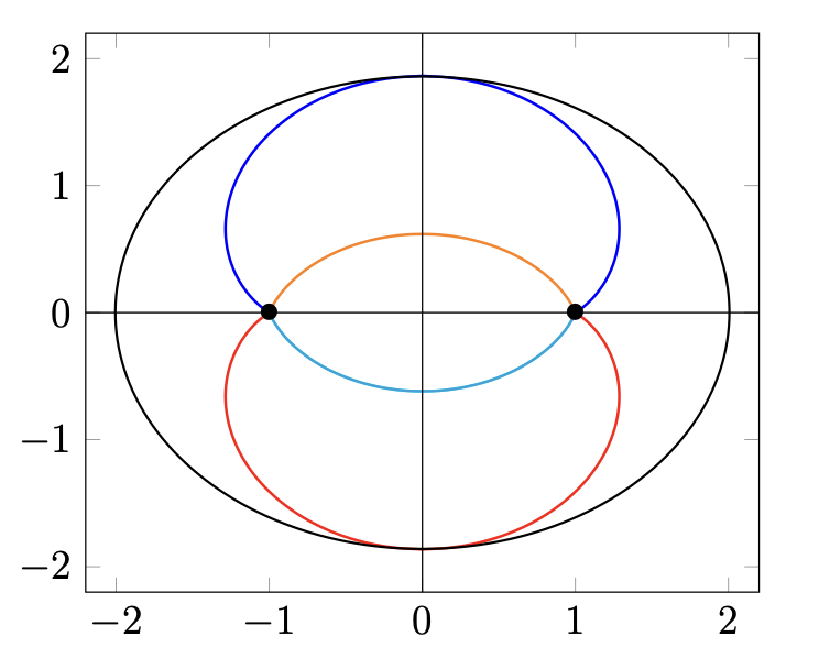
At the ${\mathbb{Z}}_{2N}$ point we have $A(x)=x^{N}$ so that the SW curve $y^{2}=x^{2N}-1$ manifestly exhibits the ${\mathbb{Z}}_{2N}$ symmetry $x\to\varepsilon x$ where $\varepsilon=e^{2\pi i/2N}$. The curve contains the two ${\mathbb{Z}}_{2N}$ symmetric points $(x,y)=(0,\pm i)$. The $2N$ branch points are given by the $2N$-th roots of unity $(x,y)=(\varepsilon^{k},0)$ for $k=0,\cdots,2N-1$, and are shown in the left panel of figure 1 for the case of $N=3$. They are mapped into one another by ${\mathbb{Z}}_{2N}$. The expansion around the ${\mathbb{Z}}_{2N}$ point is obtained by Taylor expanding the SW periods in powers of the moduli $u_{n}$. In practice, the expansion may be organized by setting,

$$y^{2}=x^{2N}-1+U(x)^{2}-2x^{N}U(x)\hskip 72.26999ptU(x)=\sum_{n=0}^{N-2}u_{n}x^{n}$$ (2.5)

and Taylor expanding $\lambda$ in powers of $U(x)$,

$$\lambda=\sum_{k=0}^{\infty}{\Gamma(k+{1\over 2})\over\Gamma({1\over 2})k!}{(2x^{N}U(x)-U(x)^{2})^{k}\over(x^{2N}-1)^{k+{1\over 2}}}\Big{(}Nx^{N}-xU^{\prime}(x)\Big{)}dx$$ (2.6)

The integrals of $\lambda$ along the homology cycles $\mathfrak{A}_{I}$ and $\mathfrak{B}_{I}$, needed in the calculation of the SW periods in (2.3), may be computed by integrating term by term in powers of $U(x)$. The homology cycles for all terms may then be chosen along the line segments of the branch cuts of the ${\mathbb{Z}}_{2N}$ symmetric curve $y^{2}=x^{2N}-1$, as illustrated in figure 1 for the case $N=3$.

As shown in [15], all such integrals may be obtained by evaluating the function $Q(\xi)$ which is defined as the Abelian integral of the SW differential, given by (2.3),

$${\pi i}\,Q(\xi)=\int_{0}^{\xi}\lambda\hskip 72.26999pt\xi^{2N}=1$$ (2.7)

between either ${\mathbb{Z}}_{2N}$ symmetric point $(x,y)=(0,\pm i)$, denoted hereby $0$, and an arbitrary branch point $(x,y)=(\xi,0)$ denoted here by $\xi$. The paths of integration are indicated in green in the left panel of figure 1. In terms of $Q(\xi)$ the SW periods are,

$$a_{I} =\sum_{J=1}^{I}\Big{\{}Q(\varepsilon^{2J-1})-Q(\varepsilon^{2J-2})\Big{\}} a_{D,I} =Q(\varepsilon^{2I})-Q(\varepsilon^{2I-1})$$ (2.8)

Swapping the roles of the ${\mathbb{Z}}_{2N}$ symmetric points $(0,\pm i)$ reverses the signs of $Q$ and all the periods which, in turn, is equivalent to a modular transformation by $-I\in{\text{Sp}}(2N-2,{\mathbb{Z}})$. The Taylor series expansion of $Q(\xi)$ in powers of the moduli $u_{n}$ is given by,

$$Q(\xi)=\sum_{\ell_{i}=0}^{\infty}\frac{2^{\frac{M-{L}}{N}}}{2\pi^{2}N}\,\xi^{NM+{L}+N}\,\Gamma\left(\tfrac{{L}}{N}\right)Y(\xi^{N},\alpha;u_{0})\,\frac{u_{1}^{\ell_{1}}\dots u_{N-2}^{\ell_{N-2}}}{\ell_{1}!\dots\ell_{N-2}!}$$ (2.9)

where we shall use the following combinations throughout,

$$L={1+}\sum_{j=1}^{N-2}j\ell_{j}\hskip 57.81621ptM=\sum_{j=1}^{N-2}\ell_{j}\hskip 57.81621pt\alpha=\frac{NM-{L}}{2N}$$ (2.10)

The function $Y(\xi^{N},\alpha;u_{0})$ is given by the following linear combination of Gauss hypergeometric functions $F={}_{2}F_{1}$,

$$Y(\xi^{N},\alpha;u_{0})= \,2u_{0}\,\xi^{N}\cos^{2}(\pi\alpha)\Gamma\left(\alpha+{\tfrac{1}{2}}\right)^{2}F\left(\alpha+{\tfrac{1}{2}},\alpha+{\tfrac{1}{2}};\tfrac{3}{2};u_{0}^{2}\right)$$

$$+\sin^{2}(\pi\alpha)\Gamma(\alpha)^{2}\,F\left(\alpha,\alpha;{\tfrac{1}{2}};u_{0}^{2}\right)$$ (2.11)

Alternatively, the hypergeometric functions may themselves be expanded in Taylor series in $u_{0}$ [15], but the above formulation will be more pertinent to the expansion around the maximal AD points, to which we now turn.

2.3 Expansion around a maximal AD point

For gauge group ${\text{SU}}(N)$ with $N\geq 3$, the maximal AD points are characterized by $u_{n}=0$ for all $n>0$ and $u_{0}=\pm 1$, recalling that we set the strong coupling scale $\Lambda=1$. Without loss of generality we may concentrate on the AD point with $u_{0}=1$ so that $A(x)=x^{N}-1$. The corresponding SW curve $y^{2}=x^{N}(x^{N}-2)$ manifestly exhibits ${\mathbb{Z}}_{N}$ symmetry $x\to\varepsilon^{2}x$, recalling that $\varepsilon=e^{2\pi i/2N}$ while the SW differential $\lambda=Nx^{N}dx/y$ transforms as $\lambda\to\varepsilon^{2}\lambda$.

2.3.1 Expansion of the SW differential

The neighborhood of the AD point $u_{0}=1$, inside of which we shall obtain a convergent series expansion, may be parametrized by first taking $u_{0}$ away from the value 1 and then turning on the moduli $u_{n}$ for $n>0$. To do so we introduce the shifted variable $v=1-u_{0}$ keeping $u_{n}=0$ for $n>0$. In terms of $v$ the SW curve is given by,

$$y^{2}=(x^{N}+v)(x^{N}+v-2)$$ (2.12)

Its branch points exhibit ${\mathbb{Z}}_{N}$ symmetry but, for $v\not=1$, do not exhibit ${\mathbb{Z}}_{2N}$ symmetry. Instead, they are given as follows for $k=0,1,\cdots,N-1$,

$$x_{k}^{+}=(2-v)^{\frac{1}{N}}\varepsilon^{2k}\hskip 72.26999ptx_{k}^{-}=v^{\frac{1}{N}}\varepsilon^{2k+1}$$ (2.13)

For sufficiently small $|v|\ll 1$ the distance from branch points to the origin is of order $\Lambda=1$ for $x^{+}_{k}$, but of order $|v|^{\frac{1}{N}}\ll 1$ for $x_{k}^{-}$, as illustarted in the right panel of figure 1 for the case $N=3$. The small branch points $x_{k}^{-}$ correspond to the intrinsic data of the AD theory, while the large branch points $x_{k}^{+}$ correspond to its embedding into ${\text{SU}}(N)$. The small branch points dominate the dynamics of the AD theory as $\Lambda\rightarrow\infty$ since the heavy states have masses of order $\Lambda$ and decouple. For $v\not=0,2$, the SW curve also contains two points that are invariant under ${\mathbb{Z}}_{N}$ given by $(x,y)=(0,\pm\sqrt{v(v-2)})$ and that are referred to simply as $0$ in figure 1.

Turning on the remaining moduli $u_{n}$ for $n>0$ will modify the disposition of the branch points from the one for the ${\mathbb{Z}}_{N}$ symmetric curve. As long as the $u_{n}$ for $n>0$ remain sufficiently small, the branch points will remain well-separated and a convergent Taylor series expansion should be expected.

In this subsection we shall evaluate the periods spanned by the small branch points, which are represented by the cycles $\mathfrak{A}_{1}^{(s)}$ and $\mathfrak{B}_{1}^{(s)}$ in the right panel of figure 1 for ${\text{SU}}(3)$, and will be defined for arbitrary ${\text{SU}}(N)$ in (2.3.2). The periods involving the large branch points, which are represented by the cycles $\mathfrak{A}_{1}^{(\ell)}$ and $\mathfrak{B}_{1}^{(\ell)}$ in the right panel of figure 1 for ${\text{SU}}(3)$, will be defined for arbitrary ${\text{SU}}(N)$ in (2.3.5) and will be evaluated in subsection 2.3.5.

Figure 1: The ${\mathbb{Z}}_{6}$ symmetric curve $y^{2}=x^{6}-1$ is shown in the left panel, while the ${\mathbb{Z}}_{3}$ symmetric curve $y^{2}=(x^{3}+v)(x^{3}+v-2)$ is shown in the right panel. In each case, the branch cuts are shown in black double lines; the integration paths for $Q(\varepsilon^{n})$ and $R(\zeta)$ are shown in green; the cycles of the canonical homology bases $\mathfrak{A}$ and $\mathfrak{B}$ are shown in blue and red, respectively.

To proceed with the evaluation of the small periods, we set $A(x)=\hat{A}(x)-1$ in terms of which the SW curve and differential become,

$$y^{2}=\hat{A}(x)(\hat{A}(x)-2)\hskip 72.26999pt\lambda={x\hat{A}^{\prime}(x)dx\over y}$$ (2.14)

The AD point $u_{0}=1$ corresponds to $\hat{A}(x)=x^{N}$ and the small branch points correspond to $|x|\ll 1$. Thus, to evaluate the periods spanned by the small branch points, we expand the denominator in powers of $\hat{A}(x)$, as follows,

$$\lambda={1\over\sqrt{-2}}\sum_{k=0}^{\infty}{\Gamma(k+{1\over 2})\over 2^{k}\,\Gamma({1\over 2})\,k!}\,{x\,\hat{A}^{\prime}(x)dx\over\hat{A}(x)^{{1\over 2}-k}}$$ (2.15)

By setting $u_{0}=1-v$ and rescaling the variable $x$ and the moduli $u_{n}$ as follows,

$$x=v^{\frac{1}{N}}z\hskip 72.26999ptu_{n}=v^{1-\frac{n}{N}}v_{n}\quad\hbox{ for }n>0$$ (2.16)

the function $\hat{A}(x)$ decomposes into a factor of $v$ times a factor that only depends on the remaining rescaled moduli $v_{n}$ for $n>0$, but is independent of $v$,

$$\hat{A}(x)=v\Big{(}z^{N}-V(z)+1\Big{)}\hskip 72.26999ptV(z)=\sum_{n=1}^{N-2}v_{n}z^{n}$$ (2.17)

Clearly, the expansion (2.14) in powers of $\hat{A}(x)$ is equivalent to an expansion in powers of $v$. To proceed, we expand $\lambda$ in powers of the remaining moduli $v_{n}$ with $n>0$ as follows,

$$\lambda={v^{{1\over 2}+\frac{1}{N}}\over\sqrt{-2}}\sum_{k=0}^{\infty}{\Gamma(k+{1\over 2})\over\Gamma({1\over 2})\,k!}\,\left({v\over 2}\right)^{k}\sum_{M=0}^{\infty}{\Gamma({1\over 2}-k+M)\over\Gamma({1\over 2}-k)\,M!}{V(z)^{M}(Nz^{N}-zV^{\prime}(z))dz\over\big{(}z^{N}+1\big{)}^{{1\over 2}-k+M}}$$ (2.18)

Note that all reference to the larger branch points has been translated into analytic dependence in $z$, and the above expression for $\lambda$ can be used only to calculate the periods spanned by the small branch points.

2.3.2 The short SW periods in terms of $R(\zeta)$

The short SW periods may be evaluated in terms of the function $R(\zeta)$ defined for $\zeta^{N}=-1$ as the integral from either one of the ${\mathbb{Z}}_{N}$ symmetric points, denoted here by $z=0$, to the small branch point $z=\zeta$ by,

$$i\pi R(\zeta)=\int_{0}^{\zeta}\lambda\hskip 72.26999pt\zeta^{N}=-1$$ (2.19)

The integral is taken along a path from $z=0$ to $z=\zeta$ that does not intersect any of the branch cuts produced by the square root, as shown in green in the right panel of figure 1. As in the case of the expansion around the ${\mathbb{Z}}_{2N}$ symmetric point, swapping the sign of the ${\mathbb{Z}}_{N}$ symmetric point amounts to reversing the sign of all periods and is equivalent to the modular transformation $-I\in{\text{Sp}}(2N-2,{\mathbb{Z}})$. The integrals $R(\zeta)$ will soon be related by analytic continuation to the integrals $Q(\xi)$ and hence to the periods $a_{I}$ and $a_{D,I}$ considered in [15]. Choosing a basis for the short homology one-cycles,

$$\hat{\mathfrak{A}}_{j}^{(s)} =[\varepsilon^{4j-3},\varepsilon^{4j-1}] \mathfrak{A}_{i}^{(s)} =\bigcup_{j=1}^{i}\hat{\mathfrak{A}}_{j}^{(s)}$$

$$\mathfrak{B}^{(s)}_{i} =[\varepsilon^{4i-1},\varepsilon^{4i+1}] i =1,\cdots\left[\tfrac{N-1}{2}\right]$$ (2.20)

the short periods $a_{i}^{(s)}$ and $a_{D,i}^{(s)}$ may be expressed in terms of the periods $a_{I}$ and $a_{D,I}$ and in terms of the function $Q(\xi)$ as follows,

$$\hat{a}_{i}^{(s)} =\hat{a}_{2i}+a_{D,2i-1}=R(\varepsilon^{4i-1})-R(\varepsilon^{4i-3}) a_{i}^{(s)} =\sum_{j=1}^{i}\hat{a}^{(s)}_{j}$$

$$a_{D,i}^{(s)} =\hat{a}_{2i+1}+a_{D,2i}=R(\varepsilon^{4i+1})-R(\varepsilon^{4i-1}) i =1,\cdots\left[\tfrac{N-1}{2}\right]$$ (2.21)

The short homology cycles $\mathfrak{A}_{1}^{(s)}$ and $\mathfrak{B}_{1}^{(s)}$ are indicated in figure 1 for ${\text{SU}}(3)$.

2.3.3 Expansion of $R(\zeta)$ and the short periods

We are now ready to formulate and prove one of the fundamental results of this paper, namely the expansion of the short periods around the maximal AD points for arbitrary gauge group ${\text{SU}}(N)$. As shown in the preceding subsection, the periods are given by (2.3.2) in terms of the function $R(\zeta)$ defined in (2.19). The results below give the expansion of the function $R(\zeta)$ around the maximal AD points.

Theorem 2.1.

The function $R(\zeta)$ for the small branch points $\zeta$ with $\zeta^{N}=-1$ admits the following series expansion around $v_{n}=0$ for all $n=1,\dots,N-2$ and $v_{0}\equiv v=1-u_{0}\neq 0$:

$$R(\zeta) =\frac{v^{{1\over 2}+\frac{1}{N}}}{\sqrt{2\pi}N}\sum_{{\ell_{n}=0\atop n=0,\cdots,N-2}}^{\infty}\frac{(-)^{M+1}\zeta^{L}\Gamma(\frac{L}{N})\Gamma(\ell_{0}+{1\over 2})^{2}}{\Gamma({1\over 2})^{2}\Gamma(\frac{3}{2}-2\alpha+\ell_{0})}\,\frac{v_{0}^{\ell_{0}}\dots v_{N-2}^{\ell_{N-2}}}{2^{\ell_{0}}\,\ell_{0}!\dots\ell_{N-2}!}$$ (2.22)

where the combinations $L,M$ and $\alpha$ were defined in (2.10).

The proof proceeds from the SW differential $\lambda$ in (2.18) and is relegated to Appendix A.

Corollary 2.2.

The summation over $\ell_{0}$ in the Taylor series expansion for $R(\zeta)$ for the small branch points with $\zeta^{N}=-1$ in Theorem 2.1 may be carried out in terms of an infinite series of Gauss hypergeometric functions ${}_{2}F_{1}=F$ and the result is given by,

$$R(\zeta) =\frac{v^{{1\over 2}+\frac{1}{N}}}{\sqrt{2\pi}N}\sum_{{\ell_{n}=0\atop n=1,\cdots,N-2}}^{\infty}W_{L,M}(\zeta,v)\,\frac{{v}_{1}^{\ell_{1}}\dots v_{N-2}^{\ell_{N-2}}}{\ell_{1}!\dots\ell_{N-2}!}$$ (2.23)

where $L,M$ were defined in (2.10) and the coefficient functions $W_{L,M}(\zeta,v)$ are given by,

$$W_{L,M}(\zeta,v) =\frac{(-)^{M+1}\,\zeta^{L}\,\Gamma(\tfrac{L}{N})}{\Gamma(\tfrac{3}{2}-2\alpha)}F({\tfrac{1}{2}},{\tfrac{1}{2}};\tfrac{3}{2}-2\alpha;\tfrac{v}{2}).$$ (2.24)

In the special case where ${v}_{n}=0$ for all $n\neq 0$, the function $R(\zeta)$ reduces to,

$$R(\zeta)=-\frac{\zeta\,v^{{1\over 2}+\frac{1}{N}}\,\Gamma(\frac{1}{N})}{\sqrt{2\pi}N\,\Gamma(\frac{3}{2}+\frac{1}{N})}F({\tfrac{1}{2}},{\tfrac{1}{2}};\tfrac{3}{2}+\tfrac{1}{N};\tfrac{v}{2}).$$ (2.25)

The corollary readily follows from Theorem 2.1, and its proof is left to the reader.

2.3.4 Evaluating $R(\zeta)$ by analytic continuation of $Q(\xi)$ for $\xi^{N}=-1$

Before addressing the calculation of the long periods, we show that $R(\zeta)$ may be obtained from $Q(\xi)$ by analytic continuation in the variable $v=1-u_{0}$ for the small branch points, namely $\xi=\zeta$ for which $\zeta^{N}=-1$. Using these results, we shall then use the same analytic continuation to obtain the long periods in the next subsection. We begin by proving the following corollary of Theorem 2.1.

Corollary 2.3.

The function $R(\zeta)$ is the analytic continuation in the modulus $v=1-u_{0}$ of $Q(\xi)$ for the small branch points specified by $\xi=\zeta$ and $\xi^{N}=-1$.

To prove the theorem, we start from the Taylor series expansion (2.9) for $Q(\xi)$ and re-express the coefficient functions $Y$ of (2.2) using the reflection formula for the $\Gamma$-function,

$$\Gamma(z)\Gamma(1-z)\sin(\pi z)=\pi$$ (2.26)

as well as the change of variables $v=1-u_{0}$,

$$Y(\xi^{N},\alpha;u_{0})=-\xi^{N}{\pi^{2}\,f_{3}(\alpha,v)\over\Gamma({\tfrac{1}{2}}-\alpha)^{2}}+{\pi^{2}\,f_{4}(\alpha,v)\over\Gamma(1-\alpha)^{2}}$$ (2.27)

in terms of the functions $f_{3}$ and $f_{4}$ given by,

$$f_{3}(\alpha,v) = -2\,(1-v)F\left(\alpha+{\tfrac{1}{2}},\alpha+{\tfrac{1}{2}};\tfrac{3}{2};(1-v)^{2}\right)$$

$$f_{4}(\alpha,v) = F\left(\alpha,\alpha;\tfrac{1}{2};(1-v)^{2}\right)$$ (2.28)

By construction, both functions admit a convergent Taylor series expansion around the point $v=1$, which is the ${\mathbb{Z}}_{2N}$ symmetric point. Our goal is to perform an analytic continuation to functions that admit convergent Taylor series expansions around the point $v=0$, which is one of the AD points. To proceed, it is readily verified that both functions $f_{3},f_{4}$ are solutions to the same hypergeometric differential equation,

$$v(2-v)\frac{d^{2}f}{dv^{2}}+(4\alpha+1)(1-v)\frac{df}{dv}-4\alpha^{2}f=0$$ (2.29)

The solutions to this equations may alternatively be expressed in terms of hypergeometric functions with argument $v/2$, whose normalizations are conveniently chosen as follows,

$$f_{1}(\alpha,v) = {2\,(2v)^{{1\over 2}-2\alpha}\over 1-4\alpha}F\left({\tfrac{1}{2}},{\tfrac{1}{2}};\tfrac{3}{2}-2\alpha;\tfrac{v}{2}\right)$$

$$f_{2}(\alpha,v) = F(2\alpha,2\alpha;2\alpha+{\tfrac{1}{2}};\tfrac{v}{2})$$ (2.30)

The two bases of solutions to (2.29) are related by a matrix ${\cal S}\in{\text{SL}}(2,{\mathbb{R}})$,

$$\left(\begin{matrix}f_{1}(\alpha,v)\cr f_{2}(\alpha,v)\cr\end{matrix}\right)={\cal S}\left(\begin{matrix}f_{3}(\alpha,v)\cr f_{4}(\alpha,v)\cr\end{matrix}\right)\hskip 72.26999pt{\cal S}=\left(\begin{matrix}{\cal S}_{13}&{\cal S}_{14}\\ {\cal S}_{23}&{\cal S}_{24}\cr\end{matrix}\right)$$ (2.31)

The resulting expression for $f_{2}$ is the Gauss-Kummer quadratic transformation of hypergeometric functions. The matrix elements of ${\cal S}$ are given as follows,[22]

$${\cal S}_{13}(\alpha) ={\Gamma({1\over 2})\Gamma({1\over 2}-2\alpha)\over\Gamma({1\over 2}-\alpha)^{2}} {\cal S}_{14}(\alpha) ={\Gamma({1\over 2})\Gamma({1\over 2}-2\alpha)\over\Gamma(1-\alpha)^{2}}$$

$${\cal S}_{23}(\alpha) ={\Gamma({1\over 2})\Gamma({1\over 2}+2\alpha)\over\Gamma(\alpha)^{2}} {\cal S}_{24}(\alpha) ={\Gamma({1\over 2})\Gamma({1\over 2}+2\alpha)\over\Gamma({1\over 2}+\alpha)^{2}}$$ (2.32)

One verifies that indeed ${\rm det\,}({\cal S})=1$ by using the reflection relation (2.26). Inspection of the coefficients ${\cal S}_{13}$ and ${\cal S}_{14}$ reveals that, for the special case where $\xi^{N}=-1$, the combination $Y(-1,\alpha;u_{0})$ is proportional to the function $f_{1}(\alpha,v)$, namely,

$$Y(-1,\alpha;u_{0})={\pi^{2}\,f_{1}(\alpha,v)\over\Gamma({\tfrac{1}{2}})\Gamma({1\over 2}-2\alpha)}$$ (2.33)

Substituting this expression into (2.9) readily produces the expressions of Theorem 2.1 in (2.23) and (2.24), which concludes the proof of Theorem 2.3. Henceforth, we shall set $R(\zeta)=Q(\zeta)$ for $\zeta^{N}=-1$ and express the short SW periods in terms of $Q(\zeta)$.

2.3.5 Expansion of $Q(\xi)$ for the long periods by analytic continuation

Obtaining the expansion of the long SW periods around the maximal AD points directly from the integral representation of the periods is considerably more involved than the evaluation for the short periods given in Theorem 2.1. Instead of proceeding directly here, we shall take advantage of the analytic continuation of the expansion for $Q(\xi)$ for $\xi^{N}=1$ around the ${\mathbb{Z}}_{2N}$ symmetric point to obtain the long periods. The long homology cycles are chosen to be,

$$\hat{\mathfrak{A}}_{i}^{(\ell)} =\hat{\mathfrak{A}}_{2i-1}-\mathfrak{B}_{2i-1} \mathfrak{A}_{i}^{(\ell)} =\bigcup_{j=1}^{i}\hat{\mathfrak{A}}_{j}^{(\ell)}$$

$$\mathfrak{B}_{i}^{(\ell)} =-\hat{\mathfrak{A}}_{2i}+\mathfrak{B}_{2i} i =1,\cdots\left[\tfrac{N}{2}\right]$$ (2.34)

The long periods will be denoted by $a_{i}^{(\ell)}$ and $a_{D,i}^{(\ell)}$ and may be expressed as follows,

$$\hat{a}_{i}^{(\ell)} =\hat{a}_{2i-1}-a_{D,2i-1} a_{i}^{(\ell)} =\sum_{j=1}^{i}\hat{a}_{j}^{(\ell)}$$

$$a_{D,i}^{(\ell)} =-\hat{a}_{2i}+a_{D,2i} i =1,\cdots\left[\tfrac{N}{2}\right]$$ (2.35)

We alert the reader to the fact that the ranges of the index $i$ labelling the short and long cycles (and periods) coincide for odd values of $N$ but differ when $N$ is even, in which case there is one more pair of long periods than short periods. Using these definitions and (2.1) one verifies that the short and long cycles satisfy the following canonical intersection pairings,

$$\mathfrak{J}(\mathfrak{A}^{(\ell)}_{i},\mathfrak{B}_{j}^{(\ell)}) =\delta_{i,j} i,j =1,\cdots\left[\tfrac{N}{2}\right]$$

$$\mathfrak{J}(\mathfrak{A}^{(s)}_{i},\mathfrak{B}_{j}^{(s)}) =\delta_{i,j} i,j =1,\cdots\left[\tfrac{N-1}{2}\right]$$ (2.36)

while all other pairings of the cycles $\mathfrak{A}^{(\ell)}_{i},\mathfrak{B}_{j}^{(\ell)},\mathfrak{A}^{(s)}_{i}$, and $\mathfrak{B}_{j}^{(s)}$ vanish. The long and short homology cycles $\mathfrak{A}_{1}^{(\ell)},\mathfrak{B}_{1}^{(\ell)},\mathfrak{A}_{1}^{(\ell)}$ and $\mathfrak{B}_{1}^{(\ell)}$ are indicated in figure 1 for ${\text{SU}}(3)$.

The Taylor series expansion of $Q(\xi)$ for $\xi^{N}=1$ at the maximal AD point in powers of the moduli $v_{n}$ for $n>0$ is given by the following theorem.

Theorem 2.4.

The Taylor series expansion near the AD point of the function $Q(\xi)$ for $\xi^{N}=1$ is given by the following expression,

$$Q(\xi)=\sum_{{\ell_{n}=0\atop n=1,\cdots,N-2}}^{\infty}\frac{2^{M-\frac{L}{N}}}{2\pi^{2}N}\xi^{L}\Gamma(\tfrac{L}{N})Y(1,\alpha;u_{0})v^{\frac{NM-L+1}{N}}\frac{{v}_{1}^{\ell_{1}}\dots v_{N-2}^{\ell_{N-2}}}{\ell_{1}!\dots\ell_{N-2}!},$$ (2.37)

where $u_{0}=1-v$, the combinations $L,\alpha$ were defined in (2.10), and $Y(1,\alpha;u_{0})$ is given by,

$$Y(1,\alpha;u_{0})=-\Gamma({\tfrac{1}{2}})\Gamma({\tfrac{1}{2}}+2\alpha)f_{1}(\alpha,v)+{2\pi^{2}\Gamma({\tfrac{1}{2}})\Gamma({\tfrac{1}{2}}-2\alpha)\over{\Gamma(1-\alpha)^{2}\Gamma({1\over 2}-\alpha)^{2}}}f_{2}(\alpha,v)$$ (2.38)

The functions $f_{1}(\alpha,v)$ and $f_{2}(\alpha,v)$ were defined in (2.3.4). In the special case where $v_{n}=0$ for $n>0$, only the term with $\ell_{n}=0$ for $n>0$ contributes so that $L=1$, and we have,

$${Q(\xi)}=\frac{2^{-\frac{1}{N}}}{2\pi^{2}N}\,\xi\,\Gamma(\tfrac{1}{N})Y(1,-\tfrac{1}{2N};u_{0})$$ (2.39)

The proof of the theorem follows from using the relation (2.31) to re-express $Q(\xi)$.

2.4 The case of gauge group ${\text{SU}}(3)$

The ${\cal N}=2$ super-Yang-Mills theory with gauge group ${\text{SU}}(3)$ offers one of the simplest settings in which the AD theories arise. For this reason, and because one can at the same time obtain simplified and more explicit formulas for the periods than in the case of arbitrary $N$, we shall study the behavior of the ${\text{SU}}(3)$ theory in detail here. The formulas we shall obtain may also be compared with various known results available in the literature [3]. In terms of the moduli $u=u_{1}$ and $v=1-u_{0}$ the SW curve and differential are given by,

$$y^{2}=(x^{3}-ux+v)(x^{3}-ux+v-2)\hskip 72.26999pt\lambda={(3x^{3}-ux)dx\over y}$$ (2.40)

Since the two factors in $y^{2}$ have no common roots, the zeros of the discriminant of this curve obey either $4u^{3}=27v^{2}$ or $4u^{3}=27(v-2)^{2}$.

2.4.1 Series expansion of the short and long periods

Using Corollary 2.2 for $N=3$ and for the case $\xi^{3}=-1$ we obtain the following expansion for the small branch points,

$$Q(\xi)=-{v^{\frac{5}{6}}\over 3\sqrt{2}\pi}\sum_{m=0}^{\infty}\xi^{m+1}{\Gamma(\tfrac{m+1}{3})\Gamma({1\over 2})\over\Gamma(\tfrac{11-4m}{6})\,m!}\left(-{u\over v^{\frac{2}{3}}}\right)^{m}\,F({\tfrac{1}{2}},{\tfrac{1}{2}};\tfrac{11-4m}{6};\tfrac{v}{2})$$ (2.41)

while using Theorem 2.4 for $N=3$ and for the case $\xi^{3}=1$ we obtain the expansion for the large branch points,

$$Q(\xi) = \sum_{m=0}^{\infty}{2^{(2m-1)/3}\over 6}\xi^{m+1}\Gamma(\tfrac{m+1}{3}){u^{m}\over m!}\bigg{[}{\Gamma(\frac{4m-5}{6})\over\Gamma({1\over 2})^{3}}(2v)^{\frac{5-4m}{6}}F({\tfrac{1}{2}},{\tfrac{1}{2}};\tfrac{11-4m}{6};\tfrac{v}{2})$$ (2.42)

$$\hskip 115.63243pt+{2\Gamma({1\over 2})\Gamma(\frac{5-4m}{6})\over\Gamma(\frac{2-m}{3})^{2}\Gamma(\frac{7-2m}{6})^{2}}F(\tfrac{2m-1}{3},\tfrac{2m-1}{3};\tfrac{4m+1}{6};\tfrac{v}{2})\bigg{]}$$

We note that $Q(\xi)$ is analytic in $u$, but non-analytic in $v$ as it contains powers of $v^{\frac{1}{6}}$ for all values of $\xi$. For $u=0$, its dependence on $v$ is through a factor of $v^{\frac{5}{6}}$ times integer powers of $v$. This scaling behavior for small $v/\Lambda^{N}$ is consistent with the predictions of the scaling dimension $\Delta=\tfrac{6}{5}$ for the intrinsic Coulomb branch of rank 1 AD theories [23, 11, 24, 25, 26, 27, 28, 29]. We shall return to this point in later sections.

2.4.2 Analyticity of the long periods

On physical grounds, the long periods, namely those associated with the embedding of the AD theory into the ${\text{SU}}(3)$ super Yang-Mills theory, are expected to be analytic in all moduli $u,v$ for $|u|,|v|\ll 1$. The fact that this is the case is borne out by the following proposition.

Proposition 2.5.

There exists an ${\text{Sp}}(4,{\mathbb{Z}})$ electric-magnetic duality frame such that one pair of periods is analytic in the moduli $(u,v)$, while the other pair of periods carry the non-analyticities associated with the AD point.

To prove the proposition, consider the following ${\text{Sp}}(4,{\mathbb{Z}})$ duality transformation, which implements the relations (2.3.2) and (2.3.5) for the special case of $N=3$,

$$\begin{pmatrix}a^{(\ell)}\\ a^{(s)}\\ a_{D}^{(\ell)}\\ a_{D}^{(s)}\end{pmatrix} =\begin{pmatrix}1&0&-1&0\\ -1&1&1&0\\ 1&-1&0&1\\ 0&-1&0&1\end{pmatrix}\begin{pmatrix}a_{1}\\ a_{2}\\ a_{D,1}\\ a_{D,2}\end{pmatrix}$$ (2.43)

where we have suppressed the sole index $i=1$. One may verify that the corresponding cycles satisfy the canonical intersection relations of (2.3.5). It will be convenient to use the decomposition of $Q(\xi)$ into characters of ${\mathbb{Z}}_{6}$, familiar from [15],

$$Q(\xi) =\sum_{n=0}^{5}\xi^{n}Q_{n} Q_{3} =0$$ (2.44)

where we recall that $Q_{0}$ actually drops out of all SW periods (see Appendix B). Expressing the long periods in terms of the functions $Q_{n}$, we obtain,

$$a^{(\ell)} =(1+\rho)(Q_{1}-3Q_{4})-\rho(Q_{5}-3Q_{2})$$

$$a_{D}^{(\ell)} =(Q_{1}-3Q_{4})+(Q_{5}-3Q_{2})$$ (2.45)

where $\rho=\varepsilon^{2}=e^{2\pi i/3}$. The combinations $3Q_{4}-Q_{1}$ and $3Q_{2}-Q_{5}$ may be obtained using equations (• ‣ B.2) and (B.11) of appendix B, and are given by,

$$3Q_{4}-Q_{1} ={2^{1/3}\over 2\pi^{\frac{3}{2}}}\sum_{\mu=0}^{\infty}{\Gamma(2\mu-{\frac{1}{3}})^{2}\Gamma(\mu+\tfrac{1}{3})\over\Gamma(2\mu+\frac{1}{6})\,(3\mu)!}F(2\mu-\tfrac{1}{3},2\mu-\tfrac{1}{3};2\mu+\tfrac{1}{6};\tfrac{v}{2})\,{u^{3\mu}\over 2^{2\mu}}$$

$$3Q_{2}-Q_{5} ={2^{-1/3}\over 2\pi^{\frac{3}{2}}}\sum_{\mu=0}^{\infty}{\Gamma(2\mu+\frac{1}{3})^{2}\Gamma(\mu+\tfrac{2}{3})\over\Gamma(2\mu+\frac{5}{6})(3\mu+1)!}F(2\mu+\tfrac{1}{3},2\mu+\tfrac{1}{3};2\mu+\tfrac{5}{6};\tfrac{v}{2})\,{u^{3\mu+1}\over 2^{2\mu}}$$ (2.46)

Hence, it is is clear by inspection that all non-analytic behavior of the long periods completely cancels, as is expected on physical grounds.

2.4.3 ${\text{SU}}(3)$ periods via elliptic functions and modular forms

The expansion of the SW periods near the AD points for ${\text{SU}}(3)$ gauge group may be obtained in terms of elliptic functions and modular form, in parallel to the results of [15] for the expansion around the ${\mathbb{Z}}_{6}$ symmetric point. We shall adopt the notations and conventions of appendix C in [15]. The derivation of these results is analogous to the one used in section 15 of [30], and will not be presented here.

We begin by parametrizing the genus 2 curve for $N=3$ given in (2.40) as follows,

$$(2\omega)^{2}x = \wp(z|\tau)$$

$$4(2\omega)^{4}u = g_{2}(\tau)={{{\sf E}_{4}(\tau)\over 12}}$$

$$-4(2\omega)^{6}v = g_{3}(\tau)=-{{{\sf E}_{6}(\tau)\over 216}}$$ (2.47)

where the Weierstrass function $\wp(z|\tau)$ has periods $2\omega$ and $2\omega\tau$, and satisfies the relation $\wp^{\prime}(z|\tau)^{2}=4\wp(z|\tau)^{3}-g_{2}(\tau)\wp(z|\tau)-g_{3}(\tau)$, while ${\sf E}_{4}(\tau)$ and ${\sf E}_{6}(\tau)$ are the modular forms of weight 4 and 6 respectively, normalized to the value 1 at the cusp $i\infty$. In terms of the parametrization (2.4.3), the SW curve (2.40) becomes,

$$y^{2} = (4\omega)^{-12}(4\wp^{3}-g_{3}\wp-g_{3})(4\wp^{3}-g_{2}\wp-g_{3}-4(2\omega)^{6})$$ (2.48)

Suitably deformining the short cycles $\mathfrak{A}=\mathfrak{A}^{(s)}_{1}=[0,2\pi i]$ and $\mathfrak{B}=\mathfrak{B}^{(s)}_{1}=[0,2\pi i\tau]$ in order to avoid the double-pole of $\wp(z)$ at $z=0$, the elliptic integrals defined by,

$$A_{n} =\frac{1}{2\pi i}\oint_{\mathfrak{A}}dz\;\wp(z)^{n} B_{n} =\frac{1}{2\pi i}\oint_{\mathfrak{B}}dz\;\wp(z)^{n}$$ (2.49)

satisfy the following recursion that holds for $J_{k}\in\{A_{k},B_{k}\}$:

$$(8n-4)J_{n}=(2n-3)g_{2}J_{n-2}+(2n-4)g_{3}J_{n-3}$$ (2.50)

with the initial conditions $A_{0}=1$ and $B_{0}=\tau$. The solution is given by,

$$A_{n}=K_{n}+\frac{{\sf E}_{2}}{12}L_{n-1}\hskip 72.26999ptB_{n}=\tau A_{n}+\frac{1}{2\pi i}L_{n-1}$$ (2.51)

where $K_{n}$ and $L_{n}$ are modular forms of weight $2n$, determined by the recursion relation (2.50) and the initial conditions. We have $K_{1}=L_{1}=0$ and,

$$K_{0} =1 K_{2} =\tfrac{{\sf E}_{4}}{144} K_{3} =-\tfrac{{\sf E}_{6}}{2160} K_{4} =\tfrac{5\,{\sf E}_{4}^{2}}{48384} K_{5} =-\tfrac{{\sf E}_{4}\,{\sf E}_{6}}{77760}$$

$$L_{0} =1 L_{2} =\tfrac{{\sf E}_{4}}{80} L_{3} =-\tfrac{{\sf E}_{6}}{1512} L_{4} =\tfrac{7\,{\sf E}_{4}^{2}}{48384} L_{5} =-\tfrac{29\,{\sf E}_{4}\,{\sf E}_{6}}{1330560}$$ (2.52)

The short periods are then given by expanding the SW differential in powers of $1/\omega$ as given by the following theorem, which offers a non-trivial extension of the calculation of short periods carried out to leading order in large $\Lambda$ in [16].

Theorem 2.6.

The small periods $a(\tau)=a^{(s)}_{1}(\tau)$ and $a_{D}(\tau)=a^{(s)}_{D,1}(\tau)$ admit the following Taylor series-expansion in terms of the basis $\{{\sf E}_{2},{\sf E}_{4},{\sf E}_{6}\}$ of the ring of quasi-modular forms, along with the variable $\omega$,

$$a = {-i\over\sqrt{2\pi}}\sum_{k,\ell,m=0}^{\infty}{\Gamma(k+\ell+m+{1\over 2})\over 2^{k+3\ell+3m}k!\,\ell!\,m!}{(-)^{\ell+m}\,g_{2}^{\ell}\,g_{3}^{m}\over(2\omega)^{6(k+\ell+m)+5}}\left(3A_{3k+\ell+3}-{g_{2}\over 4}A_{3k+\ell+1}\right)$$

$$a_{D} = {-i\over\sqrt{2\pi}}\sum_{k,\ell,m=0}^{\infty}{\Gamma(k+\ell+m+{1\over 2})\over 2^{k+3\ell+3m}k!\,\ell!\,m!}{(-)^{\ell+m}\,g_{2}^{\ell}\,g_{3}^{m}\over(2\omega)^{6(k+\ell+m)+5}}\left(3B_{3k+\ell+3}-{g_{2}\over 4}B_{3k+\ell+1}\right)\qquad$$ (2.53)

As a result, the following combination can be expressed in terms of modular forms $\{{\sf E}_{4},{\sf E}_{6}\}$

$$a_{D}-\tau a={-1\over(2\pi)^{\frac{3}{2}}}\sum_{k,\ell,m=0}^{\infty}{\Gamma(k+\ell+m+{1\over 2})\over 2^{k+3\ell+3m}k!\,\ell!\,m!}{(-)^{\ell+m}\,g_{2}^{\ell}\,g_{3}^{m}\over(2\omega)^{6(k+\ell+m)+5}}\left(3L_{3k+\ell+2}-{g_{2}\over 4}L_{3k+\ell}\right)$$ (2.54)

which is a locally holomorphic modular form of weight $-1$ provided $\omega$ is assigned holomorphic weight $1$ and $L_{n}$ has weight $2n$.

Remarks

1. The factor $2\omega$ in the denominator of each formula in Theorem 2.6 may be eliminated in favor of either the variables $(u,g_{2}(\tau))$ or the variables $(v,g_{3}(\tau))$ using (2.4.3) depending on whether the expansion is sought near the points $\tau=i$ or $\tau=\rho=e^{2\pi i/3}$ respectively.

2. The combination $a_{D}-\tau a$ vanishes at the AD point $\tau=\rho$, since we have $g_{2}(\rho)=0$, and the recursion relation implies $L_{3k+2}=0$ for all $k\geq 0$. Thus, at the AD point, we have $a_{D}=\tau a$, as must be the case for any rank-1 ${\mathcal{N}}=2$ SCFT.

3. The ${\mathbb{Z}}_{3}$ symmetry of the AD point fixes the modulus $\tau=\rho$ and $g_{2}(\rho)=0$. In the neighborhood of the AD point, the combination $|g_{2}(\tau)^{3}/g_{3}(\tau)^{2}|=4|u|^{3}/|v|^{2}$ is small, a condition that coincides with the original assumption for the validity of the expansion.

4. There exists a different potential superconformal fixed point at $\tau=i$ that preserves ${\mathbb{Z}}_{2}$ symmetry, and where $v=g_{3}(i)=0$ and $g_{2}(i)=(2\omega)^{4}4u$. The sum over $m$ in (2.54) then collapses to the $m=0$ contribution, the recursion relation (2.50) for $L_{n}$ may be solved, and the remaining dependence on $\omega$ may be eliminated in favor of $u$,

   $$a_{D}-\tau a=-\frac{u^{\frac{5}{4}}}{9\sqrt{\pi}}\sum_{n=0}^{\infty}\frac{2^{-10n}\,\Gamma(n+\frac{1}{4})^{2}\Gamma(n+\frac{3}{4})^{2}}{\Gamma(\frac{7}{12})\Gamma(\frac{11}{12})\Gamma(n+\frac{13}{12})\Gamma(n+\frac{17}{12})\Gamma(n+\frac{1}{2})n!}\left({u\over 3}\right)^{3n}$$ (2.55)

   The above series has radius of convergence $\absolutevalue{u}<3$. The scaling dimension of the operator corresponding to the modulus $u$ is $\Delta(u)=\frac{4}{5}<1$ is below the unitarity bound. This implies that there is no consistent way to take $\Lambda\rightarrow\infty$ such that the resulting theory is unitary and superconformal.

2.5 Remarks on the convergence of the ${\mathbb{Z}}_{N}$ expansion

In this subsection we shall discuss the convergence properties of the expansion around the maximal AD point, briefly for the ${\text{SU}}(N)$ case, and in more detail for ${\text{SU}}(3)$.

2.5.1 Heuristic analysis of the ${\text{SU}}(N)$ case

As illustrated in the right panel of figure 1 for the case of ${\text{SU}}(3)$, the branch points split into a set of small branch points of order ${\cal O}(v^{\frac{1}{N}})$ and large branch points of order ${\cal O}(\Lambda)$. The starting point for our expansion is a point in the moduli space of the Coulomb branch where $v\neq 0$ and $v_{n}=0$ for all $n>0$. The non-vanishing of $v$ guarantees that the small branch points $x^{-}_{k}$ remain well-separated. Turning on the moduli $v_{n}$ for $n\neq 0$ we observe that the parameter entering from the Taylor expansion in corollary 2.2 is $v_{n}$. The expansion will remain convergent as long as no two branch points are brought to coincide with one another, which requires the parameter $u_{n}$ to remain sufficiently small with respect to $v^{(N-n)/N}$. Thus, the conditions for convergence, derived on heuristic grounds, are as follow,

$$|v|\ll|\Lambda|^{N}\hskip 72.26999pt{|v_{n}|\ll 1}$$ (2.56)

For the case of ${\text{SU}}(3)$ we can make these bounds more precise.

2.5.2 Detailed analysis of the ${\text{SU}}(3)$ case

In appendix B.3, we provide a detailed derivation of the convergence conditions for the ${\mathbb{Z}}_{3}$ series. Here, we remark on its consequences and compare it with the ${\mathbb{Z}}_{6}$ series of [15].

1. The ${\mathbb{Z}}_{6}$ expansion converges provided the moduli satisfy the following inequalities [15],

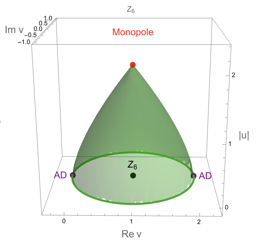
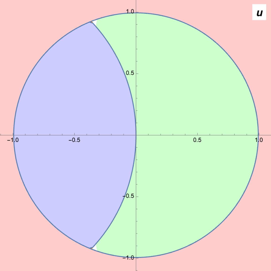
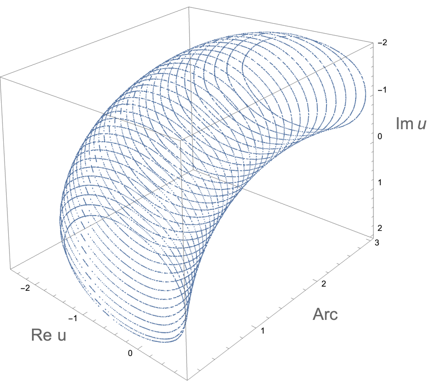
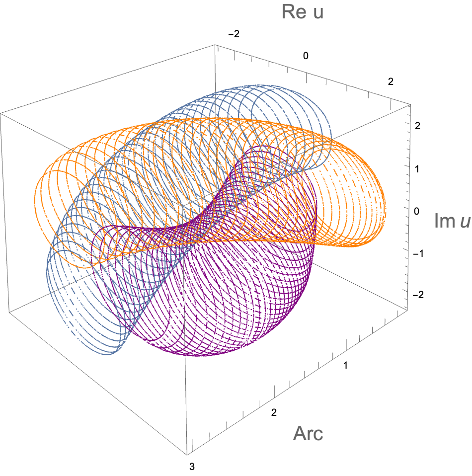
   $$\tfrac{2}{\sqrt{27}}\absolutevalue{u}^{\frac{3}{2}}+\absolutevalue{1-v}<1$$ (2.57)

   In figure 2(a), the green translucent region shows the domain of convergence of the ${\mathbb{Z}}_{6}$ expansion. The AD points are located on the boundary of this domain and the three multi-monopole points are mapped to the red dot at the peak of the conical region.

2. The ${\mathbb{Z}}_{3}$ expansion converges provided the moduli satisfy the inequalities,

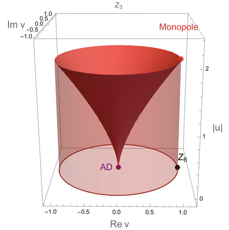
   $$\absolutevalue{\tfrac{4u^{3}}{27}}<\absolutevalue{v}^{2}<1$$ (2.58)

   In figure 2(b), the red translucent cylindrical region minus the solid cone shows the domain of convergence of the ${\mathbb{Z}}_{3}$ expansion. The AD point is at the peak of the cone. The multi-monopole and ${\mathbb{Z}}_{6}$ points are on the boundary of the domain of convergence.

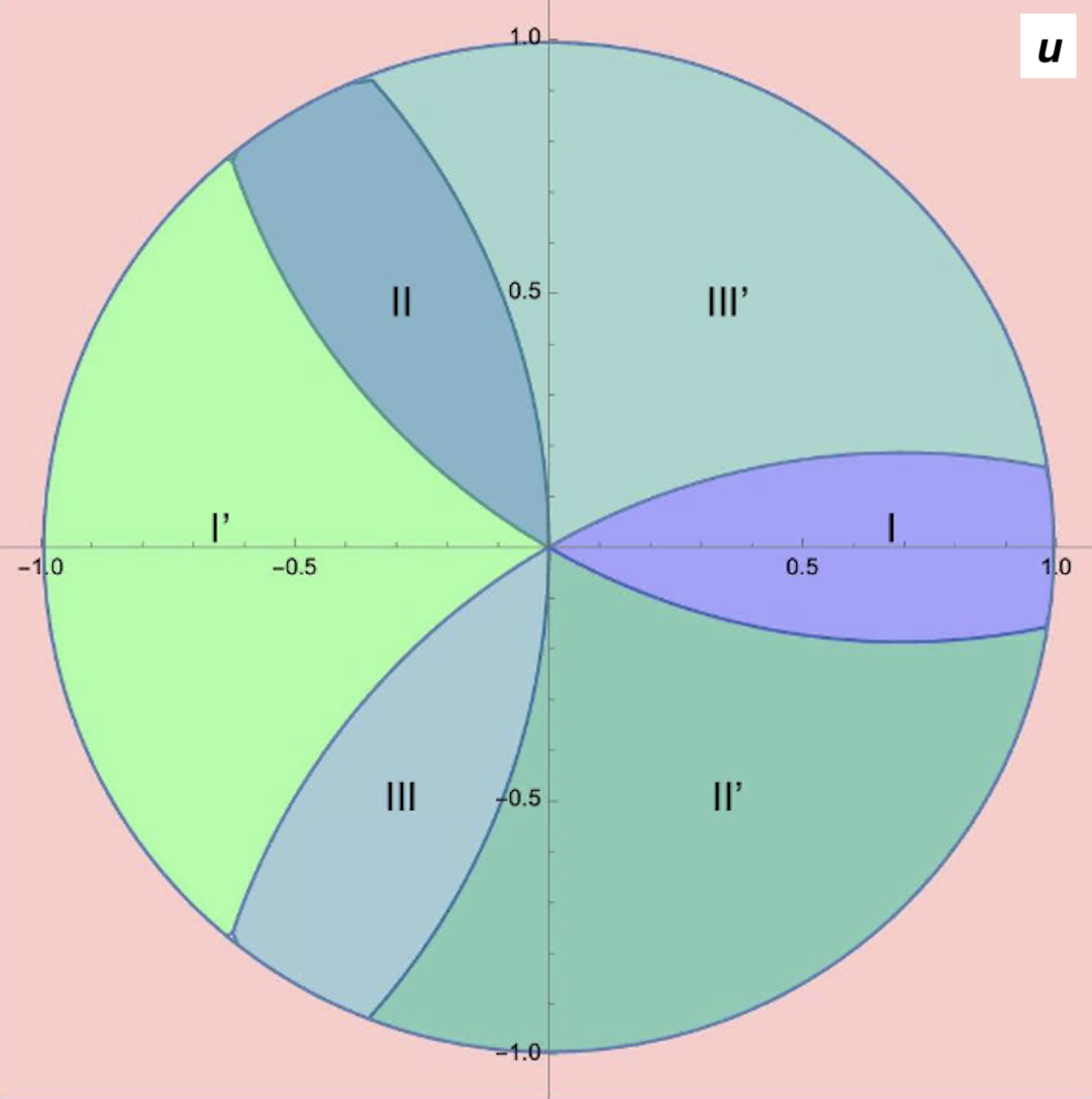
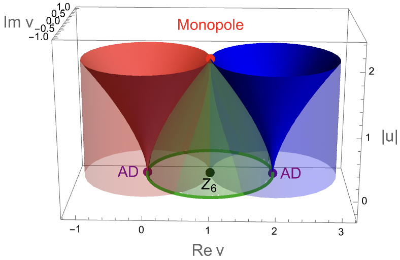
3. Figure 3 shows the total region that we can access with the combined expansions.

(a) Convergence region of ${\mathbb{Z}}_{6}$ expansion

(b) Convergence region of ${\mathbb{Z}}_{3}$ expansion

Figure 2: All the translucent colored regions denote convergence in the coordinates $({\rm Re\,}v,{\rm Im\,}v,\absolutevalue{u})$, but the opaque colored regions are excluded by convergence.

Figure 3: This plot shows the total region of moduli-space that we can access using the two ${\mathbb{Z}}_{3}$ and ${\mathbb{Z}}_{6}$ expansions: the solid blue and red cones are excluded from the regions of convergence of the ${\mathbb{Z}}_{3}$ expansions, and the translucent regions denote convergence.

3 Candidate walls of marginal stability revisited

In this section, we shall reanalyze the candidate walls of marginal stability proposed in [15] for ${\text{SU}}(3)$, this time from the perspective of the expansion of the periods around the AD points. We shall check agreement of the results obtained by the two expansions on the slice with $u=0$ and map out more walls of marginal stability beyond the $v$-plane for ${\text{SU}}(3)$, and analyze marginal stability in the ${\text{SU}}(4)$ case on the slice $u_{1}=u_{2}=0$.

3.1 Setup

In this subsection, we shall briefly summarize the setup of [15] used to analyze the marginal stability of BPS states. At a generic point on the Coulomb branch, the ${\text{SU}}(N)$ gauge-group is spontaneously broken to its maximal Abelian subgroup ${\text{U}}(1)^{N-1}$. With respect to this unbroken gauge group, the states in the theory carry both electric charges ${\bf q}=(q_{1},\cdots,q_{N-1})$ and magnetic charges ${\bf g}=(g_{1},\cdots,g_{N-1})$, which we shall assemble into a single multiplet,

$$\mu=({\bf q},{\bf g})=(q_{1},\dots,q_{N-1};g_{1},\dots,g_{N-1})\in{\mathbb{Z}}^{N-1}\times{\mathbb{Z}}^{N-1}$$ (3.1)

The central charge $Z[\mu]$ of the ${\cal N}=2$ supersymmetry algebra, evaluated in a state with charge vector $\mu$, is a linear function of $\mu$ given by [1],

$$Z[\mu]=\sum_{I=1}^{N-1}(q_{I}a_{I}+g_{I}a_{D,I})$$ (3.2)

In a unitary theory the mass $M$ of any state with charge vector $\mu$ satisfies the BPS bound $\absolutevalue{Z[\mu]}\leq M$. The state is a BPS state provided its mass $M$ saturates the BPS bound,

$$M=\absolutevalue{Z[\mu]}$$ (3.3)

Two BPS states with charges $\mu=({\bf q},{\bf g})$ and $\mu^{\prime}=({\bf q}^{\prime},{\bf g}^{\prime})$ obey the Dirac quantization condition $D\in{\mathbb{Z}}$ where $D$ is given by the symplectic pairing of the charges $\mu$ and $\mu^{\prime}$,

$$D={\bf q}\cdot{\bf g}^{\prime}-{\bf g}\cdot{\bf q}^{\prime}=\sum_{I=1}^{N-1}\Big{(}q_{I}g_{I}^{\prime}-q_{I}^{\prime}g_{I}\big{)}$$ (3.4)

When $D=0$, one may perform an ${\text{Sp}}(2N-2,{\mathbb{Z}})$ duality transformation to new charges $\tilde{\mu}$ and $\tilde{\mu}^{\prime}$ that have vanishing magnetic components, and are therefore mutually local. By contrast, when $D\not=0$, the corresponding BPS states are mutually non-local. This non-locality is, of course, familiar in the semi-classical limit where electric charges are light and magnetic monopoles are heavy soliton states such as the ‘t Hooft-Polyakov monopole. The novelty of the AD theories is the presence of massless mutually non-local states and fields.

Two BPS states with charges $\mu,\mu^{\prime}$ and masses $M=\absolutevalue{Z[\mu]},M^{\prime}=\absolutevalue{Z[\mu^{\prime}]}$, respectively, can form a bound state of charge $\mu+\mu^{\prime}$ provided the mass $M_{b}$ of the bound state satisfies $M_{b}<M+M^{\prime}$. The mass $M_{b}$ satisfies the BPS bound $\absolutevalue{Z[\mu+\mu^{\prime}]}\leq M_{b}$. In general, the inequality will be a strict one and the resulting bound state will not be a BPS state. For special charge arrangements and for special values of the vacuum expectation values $a_{I}$ and $a_{D,I}$, however, two BPS states can form a BPS bound state, namely when,

$$Z[\mu^{\prime}]=r\,Z[\mu]\hbox{ for some }r\in{\mathbb{R}}$$ (3.5)

For a given pair $\mu,\mu^{\prime}$, the solutions to this equation carve out a real co-dimension one slice of the Coulomb branch that we refer to as a candidate wall of marginal stability. Having equality of the mass $M$ of the bound state with its BPS bound $\absolutevalue{Z[\mu+\mu^{\prime}]}$ on the wall does open the option of forming a stable non-BPS bound state on either side of the wall. Whether this option is actually adopted by the theory is a dynamical question that goes beyond the purely kinematical considerations used here. For this reason the terminology candidate wall of marginal stability will be used throughout.

3.2 Marginal stability of BPS states in ${\text{SU}}(3)$

Candidate walls of marginal stability were analyzed in [15] for ${\text{SU}}(3)$ on the slice $u=0$ for arbitrary $v$ using the ${\mathbb{Z}}_{6}$ expansion of the periods. In this subsection, we re-examine these candidate walls of marginal stability using the ${\mathbb{Z}}_{3}$ expansion around one or the other of the AD points, first for $u=0$ and then for arbitrary $u,v$.

3.2.1 The $u=0$ slice

In terms of our expansion around the AD point $u_{0}=1$, given in (2.42), (2.41) and (2.44), the expressions for the SW periods of (2.8) for the case $N=3$ are as follows,

$$a_{1} =(\rho-1)(Q_{1}-Q_{4})-(3Q_{4}-Q_{1}) a_{2} =(1+\rho)a_{1}$$

$$a_{D,1} =(\rho-1)(Q_{1}-Q_{4})+\rho(3Q_{4}-Q_{1}) a_{D,2} =\rho a_{D,1}$$ (3.6)

where $\rho=e^{\frac{2\pi i}{3}}$. Consider BPS states with charge vectors $\mu=(q_{1},q_{2};g_{1},g_{2})$ and $\mu^{\prime}=(q_{1}^{\prime},q_{2}^{\prime};g_{1}^{\prime},g_{2}^{\prime})$ and corresponding central charges,

$$Z[\mu^{\prime}] =\alpha Q_{1}+\beta Q_{4}$$

$$Z[\mu] =\gamma Q_{1}+\delta Q_{4}$$ (3.7)

where we have defined the following integers of the ring ${\mathbb{Z}}[\rho]$,

$$\alpha = \rho\,(q_{1}^{\prime}-g_{2}^{\prime})-(q_{2}^{\prime}+g_{1}^{\prime})$$

$$\beta = -(2+\rho)(q_{1}^{\prime}+g_{2}^{\prime})-(1+2\rho)(q_{2}^{\prime}-g_{1}^{\prime})$$

$$\gamma = \rho\,(q_{1}-g_{2})-(q_{2}+g_{1})$$

$$\delta = -(2+\rho)(q_{1}+g_{2})-(1+2\rho)(q_{2}-g_{1})$$ (3.8)

We may parametrize the solutions to the equation (3.5) for the candidate wall of marginal stability in terms of the real variable $r$ as follows,

$$r ={Z[\mu^{\prime}]\over Z[\mu]}={\alpha z+\beta\over\gamma z+\delta} z(v) =\frac{Q_{1}(v)}{Q_{4}(v)}$$ (3.9)

Inverting the relation between $z$ and the real parameter $r$, for given charge assignments, will make $z$ trace arcs of circles in the complex $z$-plane that depend on the particular charge assignments of $\mu$ and $\mu^{\prime}$. The strong-coupling spectrum of ${\text{SU}}(N)$ SW theory has been worked out in [31], and the ${\text{SU}}(3)$ case is explained in Appendix E of [15]. We summarize the results in the following table.

Central charges and masses of BPS dyons near the ${\text{SU}}(3)$ AD points
Dyon charge	Central charge $Z[\mu_{kI}]$	$M(u_{0}=+1)$	$M(u_{0}=-1)$
$\mu_{01}=(-1,0;-1,0)$	$-(\rho-1)(Q_{1}+Q_{4})$	1.55632	0
$\mu_{12}=(-1,1;0,1)$	$-(2\rho+1)(Q_{1}+Q_{4})$	1.55632	0
$\mu_{21}=(0,1;1,1)$	$-(\rho+2)(Q_{1}+Q_{4})$	1.55632	0
$\mu_{02}=(0,1;0,-1)$	$(\rho-1)(Q_{1}-Q_{4})$	0	1.55632
$\mu_{11}=(1,0;-1,-1)$	$(2\rho+1)(Q_{1}-Q_{4})$	0	1.55632
$\mu_{22}=(1,-1;-1,0)$	$(\rho+2)(Q_{1}-Q_{4})$	0	1.55632

As indicated in the table, each AD point has three mutually non-local dyons that become simultaneously massless. The equation (3.5) has been solved for all possible pairs on the $u=0$ plane in [15]. We summarize these results below, and then build on them.

There are 15 distinct pairwise ratios of the six BPS states. Two sets of three of these ratios are between massless mutually non-local dyons. These ratios are independent of $Q_{1}$ and $Q_{4}$ and necessarily complex, such as for example $Z[\mu_{11}]/Z[\mu_{02}]=-\rho$. There can be no walls of marginal stability between such pairs. The remaining nine ratios are between one massive and one massless dyon, they do depend on $Q_{1}$ and $Q_{4}$ through the ratio $z=Q_{1}/Q_{4}$, and can lead to candidate walls of marginal stability. To analyze the ratios systematically, we compare the central charges in the first triplet of mutually non-local dyons $(Z[\mu_{01}],Z[\mu_{12}],Z[\mu_{21}])$ with cyclic permutations of the second triplet of mutually non-local dyons $(Z[\mu_{02}],Z[\mu_{11}],Z[\mu_{22}])$, as follows,

$$(Z[\mu_{01}],Z[\mu_{12}],Z[\mu_{21}]) = r_{1}\,(Z[\mu_{02}],Z[\mu_{11}],Z[\mu_{22}])$$

$$(Z[\mu_{01}],Z[\mu_{12}],Z[\mu_{21}]) = r_{2}\,(Z[\mu_{22}],Z[\mu_{02}],Z[\mu_{11}])$$ (3.10)

$$(Z[\mu_{01}],Z[\mu_{12}],Z[\mu_{21}]) = r_{3}\,(Z[\mu_{11}],Z[\mu_{22}],Z[\mu_{02}])$$

where $z=z(v)$ and,

$$r_{1}=-{z+1\over z-1}\hskip 57.81621ptr_{2}=-\rho{z+1\over z-1}\hskip 57.81621ptr_{3}=\rho^{2}{z+1\over z-1}$$ (3.11)

1. The reality of $r_{1}$ parametrizes a straight line segment in the complex $z$-plane that lies on the real-axis. We will not consider such walls because they are non-compact.

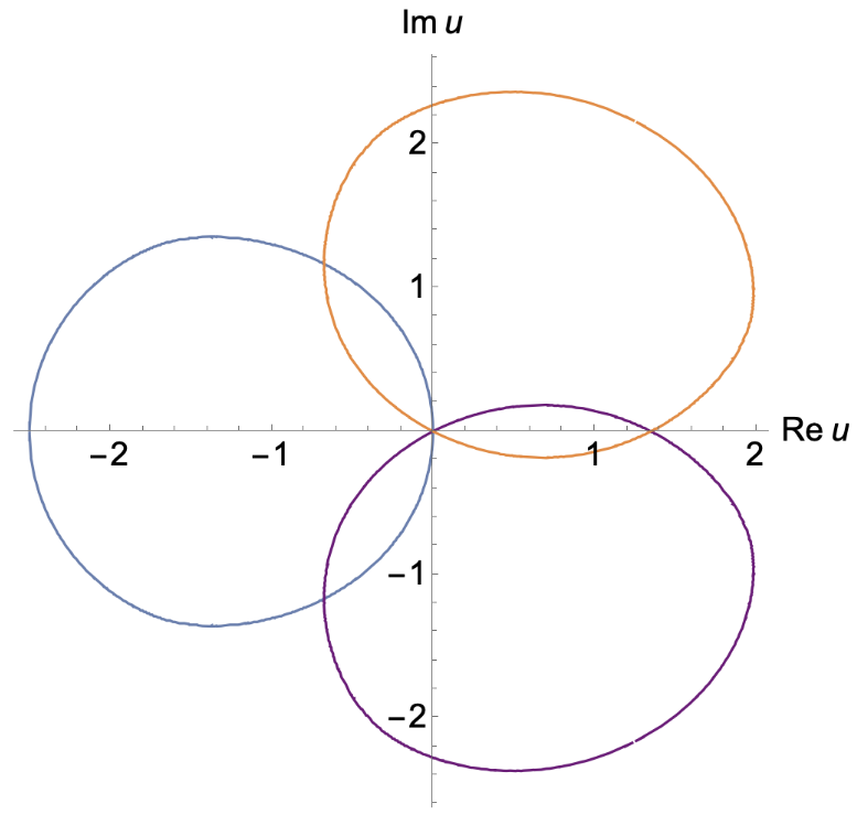
2. The reality of $r_{2}$ parametrizes a continuous subset of the circle $|z+\frac{i}{\sqrt{3}}|^{2}=\frac{4}{3}$ in the complex $z$-plane for a continuous range of values of $r_{2}\in{\mathbb{R}}$.

3. The reality of $r_{2}$ parametrizes a continuous subset of the circle $|z-\frac{i}{\sqrt{3}}|^{2}=\frac{4}{3}$ in the complex $z$-plane for a continuous range of values of $r_{3}\in{\mathbb{R}}$.

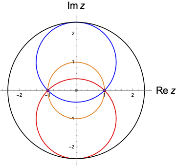
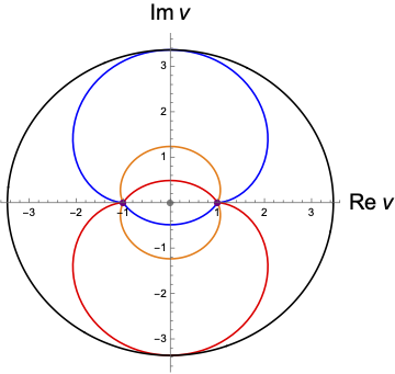
In this sense, each candidate wall of marginal stability on the $v$-plane has a three-fold degeneracy, i.e. each wall can be obtained from three distinct pairs of dyons. Finally, we can numerically map $z(v)$ to the $u_{0}$-plane by using the expression for $w(v)$ in terms of $v$ or $u_{0}$. This is displayed in the right panel of figure 4, which reproduces the result of [15]

Figure 4: The candidate walls of marginal stability for ${\text{SU}}(3)$ on the slice $u=0$ are represented by colored arcs in the $z$-plane in the left panel and in the $u_{0}$ plane in the right panel. The contour of vanishing Kähler potential is drawn in black [15].

3.2.2 Existence of walls of marginal stability away from the $v$-plane

In this sub-subsection, we give an argument for the existence of walls of marginal stability in the ${\text{SU}}(3)$ Coulomb branch with $u\neq 0$ over the curves of marginal stability restricted to the $v$-plane. We expect to find a marginal stability subspace of real dimension three inside the Coulomb branch, since we have 2 complex degrees of freedom $u$ and $v$ parametrizing the Coulomb branch, and one real constraint $Z_{2}/Z_{1}\in{\mathbb{R}}$. Since such a surface lives in the four-dimensional moduli space, it is rather hard to visualize and we shall focus instead on the marginal stability subspace of a three-dimensional slice of the Coulomb branch that we can visualize more easily. The following proposition shows the existence of walls in the $u$-plane for fixed values of $v$ that lie on a wall.

Proposition 3.1.

For any point $v_{0}$ on a curve of marginal stability in the $v$-plane, there exists a curve of marginal stability in the $u$-plane that goes through the point $(u,v)=(0,v_{0})$.

We hold $v=v_{0}$ fixed and consider two central charges $Z_{1}(u)$ and $Z_{2}(u)$ evaluated at the point $v=v_{0}$, which may be regarded as a (locally) holomorphic function of a single complex variable $u$. Then we may define the relative phase of these two central charges as,

$$e^{2i\phi(u,\bar{u})}=\frac{Z_{1}(u)\bar{Z}_{2}(\bar{u})}{Z_{2}(u)\bar{Z}_{1}(\bar{u})}$$ (3.12)

In what follows, we will use the fact that the phase of a holomorphic function $f$ is harmonic for all points where the function is non-zero; this assumption is necessary since one takes the logarithm of $f$ in the proof of this fact. However, (potential) vanishing of the central charge $Z_{k}(u)$ does not pose an issue since we take its complex modulus in the definition of the relative phase. Then it follows that $\phi(u,\bar{u})$ is locally a harmonic function on any open set that contains $u=0$. But a harmonic function on a connected domain ${\cal D}\subset{\mathbb{C}}$ can never attain its extreme values in the interior. Any point $u_{0}\in{\mathbb{C}}$ that lies on a wall of marginal stability, i.e. $Z_{2}/Z_{1}\in{\mathbb{R}}$, satisfies $\phi(u_{0},\bar{u}_{0})=0$. In particular, $\phi(0,0)=0$. This implies that zero is neither a minimum nor a maximum of $\phi$, and that there exists a closed subset ${\cal C}\subset\partial{\cal D}$ such that $\phi({\cal C})<0$ and $\phi({\cal C}^{c})\geq 0$. Hence, there exists a curve of marginal stability that goes through the interior and is continuously connected to $u=0$.

Remark. The above proposition applies locally in a neighborhood of $u=0$, where the central charges are analytic. In particular, $Z(u)$ is not required to be analytic globally, and hence the function $\phi$ would not be globally harmonic due to the potential non-analyticities in $Z(u)$. Therefore, this local existence result for walls of marginal stability does not pose an obstruction to the compactness of the walls of marginal stability.

3.2.3 Numerically finding walls of marginal stability beyond the $v$-plane

In this sub-subsection, we will find candidate walls of marginal stability using two distinct methods: perturbation theory and numerical integration.

The first method involves first-order perturbation theory in $u$ for a fixed value of $v$ on the orange arc in figure 4 and a mesh of values of $r$. We note that the figure does not appreciably change even if we go to high orders in perturbation theory, as long as we are inside the radius of convergence.

(a) Walls for the a single pair $(\mu_{01},\mu_{22})$

(b) Walls for all three pairs

(c) Full picture of the three walls beyond the radius of convergence

Figure 5: The figure above shows the curves of marginal stability on the $u$-plane for $u_{0}\sim 0.6184i$ (the midpoint of the orange arc in figure 4). The left panel shows the walls for a single pair of dyons. The red region is inaccessible by perturbation theory since our ${\mathbb{Z}}_{6}$-expansion does not converge there, the blue region is where the BPS states $\mu_{01}$ and $\mu_{22}$ are stable with $\phi<0$, and the green region is where bound states may be formed, i.e. $\phi>0$. The right panel shows a plot of the curves of marginal stability on the $u$-plane for all three pairs of dyons simultaneously. Again, the red region is inaccessible by perturbation theory. The regions of mutual stability ($\phi<0$) and instability ($\phi>0$) for 2 pairs are: II and II^′ for $(\mu_{01},\mu_{22})$ and $(\mu_{12},\mu_{02})$, I and I^′ for $(\mu_{12},\mu_{02})$ and $(\mu_{21},\mu_{11})$, III and III^′ for $(\mu_{21},\mu_{11})$ and $(\mu_{01},\mu_{22})$. The panel 5(c) displays the full walls beyond the radius of convergence obtained from numerical integration. Blue walls correspond to $(\mu_{01},\mu_{22})$, orange walls to $(\mu_{12},\mu_{02})$, and purple walls to $(\mu_{21},\mu_{11})$.

We will focus on the segment of the curve produced by the pairs $(\mu_{01},\mu_{22})$, $(\mu_{12},\mu_{02})$, and $(\mu_{21},\mu_{11})$ that has positive imaginary part, i.e. the orange curve in figure 4. For any $u_{0}$ with $\absolutevalue{u_{0}}<1$ on this arc, we have an absolutely convergent expansion in $u$, and we can get arbitrarily close to the AD points at $u_{0}=\pm 1$. Recall that our expansions have the following radii of convergence in the $u$-plane.

$${\mathbb{Z}}_{3}\text{ points}:~{}2^{\frac{1}{3}}\absolutevalue{u} <3\absolutevalue{\pm 1\mp u_{0}}^{\frac{2}{3}}<3\text{ for }u_{0}=\pm 1\text{ respectively}$$

$${\mathbb{Z}}_{6}\text{ point}:~{}2^{\frac{2}{3}}\absolutevalue{u} <3\left(1-\absolutevalue{u_{0}}\right)^{\frac{2}{3}}\quad\text{ and }\quad\absolutevalue{u_{0}}<1.$$ (3.13)

On regions of overlapping convergence, recall that $\text{Radius}_{u}({\mathbb{Z}}_{3})\geq\text{Radius}_{u}({\mathbb{Z}}_{6})$. Hence, it is more fruitful to apply the ${\mathbb{Z}}_{3}$ expansions near the AD points because this inequality is significant. On the other hand, we apply the ${\mathbb{Z}}_{6}$ expansion on the imaginary $v$-axis because that is the boundary of convergence for the ${\mathbb{Z}}_{3}$ expansion. Precisely at the AD points, neither expansion converges but we can get arbitrarily close.

However, this method is limited by the radius of convergence of the expansion. To circumvent this limitation, we recall that the periods of pure ${\text{SU}}(3)$ SW theory satisfy Picard-Fuchs equations in the variables [7]

$$(x_{1},x_{2})=\left(\frac{4u^{3}}{27},(1-v)^{2}\right)$$ (3.14)

This system of second-order PDEs can be transformed into a system of first-order ODEs which are numerically integrable (see Appendix D of [15]). We use this method to compute the periods, central charges, and walls of marginal stability, by scanning for points on the $u$-plane, for fixed values of $v$ on the orange arc in figure 4 where $Z[\mu_{2}]/Z[\mu_{1}]$ is real-valued.

Remarks

(a) 1 pair $(\mu_{01},\mu_{22})$

(b) All $3$ pairs – degeneracy lifted

Figure 6: A three-dimensional view of the candidate walls of marginal stability.

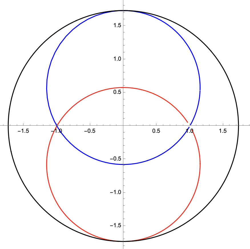
1. The three pairs correspond to the three walls in figure 5, both related by ${\mathbb{Z}}_{3}$. At the fixed point $u=0$ of this ${\mathbb{Z}}_{3}$ symmetry the degeneracy among the three pairs is restored.

2. The arcs in figure 5 with $\phi=0$ are approximately circular near the origin because, inside the radius of convergence, equation (3.5) was truncated to first order to give,

   $$(du-b) \approx r(-cu+a)\Rightarrow u(r)=\frac{ar+b}{cr+d}+\dots$$

   for some $a,b,c,d\in{\mathbb{C}}$ with $ad-bc\neq 0$. An equation of this form traces out an arc of a circle inside the radius of convergence. However, the arcs are slightly deformed from circles outside the radius of convergence, as is clear from figure 5(c).

3. The plots in figure 6 were created by picking 33 evenly spaced points on the orange arc of marginal stability in figure 4 and then solving numerically for $\phi=0$.

4. The region of stability is a tubular neighborhood, and there are three such compact regions corresponding to the three walls that are related by ${\mathbb{Z}}_{3}$.

3.3 Marginal stability of BPS states in ${\text{SU}}(4)$

On the slice that contains the AD points (i.e. $u_{k}=0$ for $k\neq 0$), we have

$$a_{1} =\varepsilon Q_{-}-Q_{+} a_{D,1} =\varepsilon^{2}Q_{+}-\varepsilon Q_{-}$$

$$a_{2} =(\varepsilon^{2}+1)a_{1} a_{D,2} =\varepsilon^{2}a_{D,1}$$ (3.15)

$$a_{3} =\varepsilon^{2}a_{1} a_{D,3} =-a_{D,1}$$

The central charge can be shown to take the following form ($Q_{\pm}=Q_{1}\pm Q_{5}$):

$$Z[\mu] =(m_{0}+\varepsilon^{2}m_{2})Q_{+}+\varepsilon(n_{0}+\varepsilon^{2}n_{2})Q_{-},$$ (3.16)

where

$$m_{0} =-q_{1}-q_{2}-g_{2} n_{0} =q_{1}+q_{2}-g_{1}+g_{3}$$

$$m_{2} =-q_{2}-q_{3}+g_{1}-g_{3} n_{2} =q_{2}+q_{3}-g_{2}$$

As for ${\text{SU}}(3)$, the following coordinate will be convenient

$$z(v)=\frac{Q_{1}}{Q_{5}}$$ (3.17)

The strong-coupling spectrum of BPS dyons in pure ${\mathcal{N}}=2\;{\text{SU}}(N)$ gauge theory was worked out in [31]. Following their algorithm for the $N=4$ case, we see that there are 12 stable BPS dyons at strong coupling which split into 2 sets of 6, each of which becomes massless at one or the other of the two AD points corresponding to $(u_{0},u_{1},u_{2})=(\pm 1,0,0)$. Two dyons within each set of 6 are mutually local, while two dyons belonging to different sets of 6 are mutually non-local. The electromagnetic charge vectors $\mu_{kJ}=(q_{1},q_{2},q_{3};g_{1},g_{2},g_{3})$ for the IR gauge-group ${\text{U}}(1)_{1}\times{\text{U}}(1)_{2}\times{\text{U}}(1)_{3}$ are displayed in the table that follows.

Masses and central charges of BPS dyons near the ${\text{SU}}(4)$ maximal AD points
Dyon	$Z[\mu_{kI}]$	$M(u_{0}=+1)$	$M(u_{0}=-1)$
$\mu_{01}=(-1,0,0;-1,0,0)$	$(1-\varepsilon^{2})Q_{+}$	1.2828	0
$\mu_{03}=(0,1,-1;0,0,-1)$	$-(1-\varepsilon^{2})Q_{+}$	1.2828	0
$\mu_{12}=(-1,1,0;0,1,0)$	$-(1+\varepsilon^{2})Q_{+}$	1.2828	0
$\mu_{32}=(0,0,1;1,1,1)$	$-(1+\varepsilon^{2})Q_{+}$	1.2828	0
$\mu_{21}=(0,1,0;1,1,0)$	$-2Q_{+}$	1.8142	0
$\mu_{23}=(-1,0,1;0,1,1)$	$-2\varepsilon^{2}Q_{+}$	1.8142	0
$\mu_{02}=(0,1,-1;0,-1,0)$	$\varepsilon(1+\varepsilon^{2})Q_{-}$	0	1.2828
$\mu_{22}=(1,0,0;-1,-1,-1)$	$\varepsilon(1+\varepsilon^{2})Q_{-}$	0	1.2828
$\mu_{31}=(0,0,1;0,0,-1)$	$-\varepsilon(1-\varepsilon^{2})Q_{-}$	0	1.2828
$\mu_{33}=(1,-1,0;-1,0,0)$	$\varepsilon(1-\varepsilon^{2})Q_{-}$	0	1.2828
$\mu_{11}=(1,0,-1;-1,-1,0)$	$2\varepsilon Q_{-}$	0	1.8142
$\mu_{13}=(0,1,0;0,-1,-1)$	$2\varepsilon^{3}Q_{-}$	0	1.8142

We observe a phenomenon that did not occur in ${\text{SU}}(3)$: at each AD point, the massive BPS states belong to two different multiplets with unequal masses $m_{0}=1.2828$ and $m_{1}=1.8142$, listed explicitly below.

• IA. Massless at $u_{0}=1$ but have mass $m_{0}$ at $u_{0}=-1$: $\{\mu_{02},\mu_{22},\mu_{31},\mu_{33}\}$.

• IB. Massless at $u_{0}=1$ but have mass $m_{1}$ at $u_{0}=-1$: $\{\mu_{11},\mu_{13}\}$.

• IIA. Massless at $u_{0}=-1$ but have mass $m_{0}$ at $u_{0}=1$: $\{\mu_{01},\mu_{03},\mu_{12},\mu_{32}\}$.

• IIB. Massless at $u_{0}=-1$ but have mass $m_{1}$ at $u_{0}=1$: $\{\mu_{21},\mu_{23}\}$.

Naïvely, there are $\binom{12}{2}$ distinct pairs. But ratios of central charges within a single category always give rise to trivial walls of complex-co-dimension 1 in the $z$-plane. So, it suffices to consider walls between distinct types: $\{$IA-IIA, IA-IIB, IB-IIA, IB-IIB$\}$. Hence, there are only $36$ pairs between mutually local BPS states that could give rise to genuine walls.

1. IA-IIA. We have the folllowing candidate walls for this case:

   $$z_{1}(r)=\frac{1+\alpha r}{1-\alpha r},\;\text{where }\alpha\in\{\pm\varepsilon,\pm i\varepsilon\}.$$ (3.18)

2. IB-IIA. We have the folllowing candidate walls for this case:

   $$z_{2}(r)=\frac{1+\beta r}{1-\beta r},\;\text{where }\beta\in\{\pm\tfrac{1}{\sqrt{2}},\pm\tfrac{i}{\sqrt{2}}\}.$$ (3.19)

3. IA-IIB. We have the folllowing candidate walls for this case:

   $$z_{3}(r)=\frac{1+\gamma r}{1-\gamma r},\;\text{where }\gamma\in\{\pm\sqrt{2},\pm i\sqrt{2}\}.$$ (3.20)

4. IB-IIB. We have the folllowing candidate walls for this case:

   $$z_{4}(r)=\frac{1+\delta r}{1-\delta r},\;\text{where }\delta\in\{-\varepsilon^{\pm 1}\}.$$ (3.21)

Figure 7: The candidate walls of marginal stability for the ${\text{SU}}(4)$ case on the slice $u_{1}=u_{2}=0$ represented in the $z$-plane in the left panel and in the $v$-plane in the right panel. The purple dots denote the AD points, and the gray dot is the ${\mathbb{Z}}_{8}$-point. The black curve is the contour of vanishing Kähler potential.

This set of curves is still highly degenerate: there are only three distinct walls of marginal stability.

1. A circle of radius $\sqrt{2}$ centred at $z=i$ with degeneracy $10$.

2. A circle of radius $\sqrt{2}$ centred at $z=-i$ with degeneracy $10$.

3. A circle of radius $1$ centred at $z=0$ with degeneracy $12$.

Note that the above degeneracy adds up to $32$ instead of $36$ since we do not consider the straight lines with degeneracy $4$ corresponding to $\beta=\pm\frac{1}{\sqrt{2}}$ and $\gamma=\pm\sqrt{2}$. The last contour to plot is of vanishing Kähler potential:

$$K(v)=0\Rightarrow\absolutevalue{z}=\cot(\frac{\pi}{8})=1+\sqrt{2}.$$ (3.22)

3.4 Comments on the ${\text{SU}}(N)$ case for $u_{k}=0$ for $k>0$

We have computed candidate walls of marginal stability up to ${\text{SU}}(7)$ on the $v$-plane with $u_{k}=0$ for $k>0$. We do not give the pictures here explicitly since they share many features. Instead, we close this section with some general remarks on the ${\text{SU}}(N)$ case, always assuming $u_{k}=0$ for $k>0$ in what follows. A generic wall of marginal stability on this slice satisfies

$$z(r)=\frac{Q_{1}}{Q_{N+1}}=\frac{\alpha r+1}{\alpha r-1},\text{ for some }\alpha\in{\mathbb{C}}\text{ and any }r\in{\mathbb{R}}.$$ (3.23)

The Kähler potential on such a wall of marginal stability satisfies [15]

$$K(v)|_{\text{wall}}=\frac{N}{2\pi}\absolutevalue{Q_{N+1}}^{2}\tan(\tfrac{\pi}{2N})\left[\absolutevalue{\frac{\alpha r+1}{\alpha r-1}}^{2}-\cot^{2}\left(\tfrac{\pi}{2N}\right)\right].$$ (3.24)

Since $r$ can be arbitrarily rescaled, without loss of generality, we may take $\alpha=e^{i\phi}\in S^{1}$, for $\phi\in[0,\pi]$ (we identify $\alpha\sim-\alpha$ since they are equivalent under $\zeta\mapsto-\zeta$). For the present discussion, we suppose that $\alpha\notin\{0,\pi\}$ so that we exclude straight lines on the real axis.

Consider the special case $\alpha=i$. Then we have $\absolutevalue{z}=1$. This is the origin-centred circle in the $z$-plane that exist for $N=2,4,6$. For the $N=2$ case, this is precisely the $K=0$ contour found by Seiberg and Witten [1]. However, such an origin-centred circle seems to be absent for odd $N$ – we checked this up to ${\text{SU}}(7)$ but lack a proof.

If a wall of marginal stability that is confined to the region $K\leq 0$ contains a point where $K=0$, then we claim that it must be tangential to the $K=0$ contour at one of $z=\pm i\cot(\frac{\pi}{2N})$. This point, together with both the AD points, uniquely specifies a circle in the $z$-plane. This can be seen explicitly by setting (3.24) to zero, which amounts to

$$(1-\cot^{2}(\tfrac{\pi}{2N}))r^{2}+2\csc^{2}(\tfrac{\pi}{2N})\cos\phi r+(1-\cot^{2}(\tfrac{\pi}{2N}))=0.$$ (3.25)

This discriminant of this quadratic polynomial is

$$D=2\csc^{4}(\tfrac{\pi}{2N})(\cos(2\phi)-\cos(\tfrac{2\pi}{N})).$$ (3.26)

This equation admits real solutions provided $\phi\in[0,\frac{\pi}{N}]\cup[\pi-\frac{\pi}{N},\pi]$. If $\phi\notin\{\frac{\pi}{N},\pi-\frac{\pi}{N}\}$, the wall intersects the $K=0$ contour twice. Such a wall goes beyond the $K\leq 0$ region since the circle also goes through the AD points; i.e. this is a circle through four specified points. If $\phi\in\{\frac{\pi}{N},\pi-\frac{\pi}{N}\}$, then $D=0$ and we have a unique intersection corresponding to $\alpha=e^{\pm i\frac{\pi}{N}}=\varepsilon^{\pm 1}$. Solving the quadratic for these values of $\alpha$ fixes $r=\pm 1$, i.e. $z=\pm i\cot(\tfrac{\pi}{2N})$. Hence, there exist only two distinct walls of marginal stability that are confined to the region $K\leq 0$, and are tangential to the contour $K=0$. Furthermore, such walls exist for all $N\geq 3$. However, the above statement does not preclude the existence of walls that are confined to the strong-coupling region but always have $K<0$. This pair of walls is explicitly realized in the cases $N=3,4,5,6,7$.

The contour of vanishing Kähler potential is also a universal feature, and always has radius $\cot(\frac{\pi}{2N})$ in the $z$-plane, which scales like $\sim N$ as $N\rightarrow\infty$. This $N$-scaling of the radius of the $K=0$ contour implies that the universal curves of marginal stability that are tangential to the $K=0$ contour do not exist at large-$N$ since they tend to straight lines. On the other hand, for any even $N$, we always expect to find the contour with $\absolutevalue{z}=1$ since its radius is independent of $N$. The fate of the other contours (in the strict region $K<0$) for even or odd $N$ is not completely clear. We expect that the even and odd cases converge to the same picture as $N\rightarrow\infty$. On these grounds, we suspect that the contours that lie in the (strict) $K<0$ region for any $N$ converge to the contour with $\absolutevalue{z}=1$ as $N\rightarrow\infty$, but we do not have a proof. We close with an open question: is $\absolutevalue{z}=1$ the unique contour of marginal stability as $N\rightarrow\infty$ on the $z$-plane with $u_{k}=0$ for $k\neq 0$?

4 The intrinsic Coulomb branch of AD theories

In this section we shall study certain properties of the intrinsic Coulomb branch of the AD theories by taking the $\Lambda\to\infty$ limit of the asymptotically free embedding ${\text{SU}}(N)$ super Yang-Mills theory near one of the maximal AD points. The resulting intrinsic AD theory is ${\cal N}=2$ superconformal, its operators transform under representations of the superconformal Lie algebra ${\text{SU}}(2,2|2)$, and have definite scaling dimensions. In particular, we shall study the behavior of the Kähler potential in this limit, and show that it is positive definite (vanishing only at the AD point) and convex provided only genuine intrinsic Coulomb branch operators ${\cal O}_{n}$ are turned on away from the AD point, whose operator dimension satisfies the unitarity bound $\Delta({\cal O}_{n})>1$ in a unitary superconformal field theory.

4.1 The $(\mathfrak{a}_{1},\mathfrak{a}_{N-1})$ intrinsic Coulomb branch

The intrinsic AD theories exist independently of their embedding into the Coulomb branch of an asymptotically-free parent theory, and a given AD theory may be reached from different parent theories. For example, the AD theories obtained in the $\Lambda\to\infty$ limit of the parent theories ${\text{SU}}(3)_{N_{f}=0}$ and ${\text{SU}}(2)_{N_{f}=1}$ are the same and referred to as the $(\mathfrak{a}_{1},\mathfrak{a}_{2})$ theory. The nomenclature originates with yet another parent theory, namely the $(\mathfrak{a}_{1},\mathfrak{a}_{2})$ theory may be constructed by compactifying the six-dimensional ${\cal N}=(2,0)$ theory with gauge-algebra $\mathfrak{a}_{1}$. The BPS quiver for such a theory is given by the product of the $\mathfrak{a}_{1}$ and $\mathfrak{a}_{N-1}$ Dynkin diagrams, whence the nomenclature $(\mathfrak{a}_{1},\mathfrak{a}_{N-1})$ [32, 33, 34, 35].

In this section, we shall consider the intrinsic theory obtained near the maximal AD points of the ${\cal N}=2$ super Yang-Mills theory with gauge group ${\text{SU}}(N)$ without hyper-multiplets. These theories can also be constructed The SW curve and one-form are given by, [36]

$$\hat{y}^{2} =x^{N}-\sum_{n=1}^{N-2}u_{n}x^{n}+v \lambda =\sqrt{-2}\,\hat{y}\;dx$$ (4.1)

The resulting SW curve and differential are scale covariant in the following sense. Since the SW periods are given by integrals of $\lambda$, we must assign to $\lambda$ the scaling dimension one, which means that under a scale transformation by a factor of $s\in{\mathbb{C}}^{*}$ we have $\lambda\to\lambda^{\prime}=s\lambda$. This scaling relation may be derived from the following scale transformations on $x,u_{n},v\sim u_{0}$,

$$x\to x^{\prime}=s^{\tfrac{2}{N+2}}x\hskip 43.36243pt\hat{y}\to\hat{y}^{\prime}=s^{\frac{N}{N+2}}\hat{y}\hskip 43.36243ptu_{n}\to u_{n}^{\prime}=s^{2\frac{N-n}{N+2}}u_{n}$$ (4.2)

for $n=0,1,\cdots,N-2$. The scaling dimension of the operator ${\cal O}_{n}$ whose expectation value is $u_{n}$ has the same scaling dimension as $u_{n}$ and therefore is given by,

$$\Delta({\cal O}_{n})=2{N-n\over N+2}$$ (4.3)

In a unitary superconformal field theory the dimension of every physical operator must be larger than one in view of the unitarity bound imposed by the representation theory of the supersymmetry algebra, which requires $\Delta({\cal O}_{n})>1$ and thus,

$$n+1\leq\left[\frac{N-1}{2}\right]=\mathfrak{r}$$ (4.4)

The parameter $\mathfrak{r}$ is referred to as the rank of the $(\mathfrak{a}_{1},\mathfrak{a}_{N-1})$ AD theory, and is defined to be the dimension over ${\mathbb{C}}$ of the intrinsic Coulomb branch. By contrast, the parameters $u_{n}$ for $n\geq\mathfrak{r}$ do not correspond to intrinsic moduli of the AD theory.

4.2 The intrinsic Kähler potential

The Kähler potential of ${\text{SU}}(N)$ SW theory is defined by,

$$K_{{\text{SU}}(N)}=\frac{i}{4\pi}\sum_{I=1}^{N-1}\Big{(}a_{I}\,\bar{a}_{D,I}-\bar{a}_{I}\,a_{D,I}\Big{)}$$ (4.5)

We may conveniently re-express $K_{{\text{SU}}(N)}$ in terms of the long and short periods with the help of an ${\text{Sp}}(2N-2,{\mathbb{Z}})$ change of duality frame, which results in the following expression,

$$K_{{\text{SU}}(N)}=\frac{i}{4\pi}\sum_{i=1}^{\mathfrak{r}}\left(a_{i}^{(s)}\bar{a}_{D,i}^{(s)}-\bar{a}_{i}^{(s)}a_{D,i}^{(s)}\right)+\frac{i}{4\pi}\sum_{i=1}^{\left[\tfrac{N}{2}\right]}\left(a_{i}^{(\ell)}\bar{a}_{D,i}^{(\ell)}-\bar{a}_{i}^{(\ell)}a_{D,i}^{(\ell)}\right)$$ (4.6)

where the rank $\mathfrak{r}$ was defined in (4.4). We consider the decoupling limit of the ${\text{SU}}(N)$ super Yang-Mills theory near the AD point as $\Lambda\rightarrow\infty$ to obtain the intrinsic periods and the intrinsic Kähler potential. Doing so causes the term in the Kähler potential for the long periods to vanish, leaving the intrinsic Kähler potential $K_{{\text{AD}}}$ of the AD theory expressed solely in terms of the short periods,

$$K_{\text{AD}} =\frac{i}{4\pi}\sum_{i=1}^{\mathfrak{r}}(a_{i}^{(s)}\bar{a}_{D,i}^{(s)}-\bar{a}_{i}^{(s)}a_{D,i}^{(s)})$$ (4.7)

in the limit where $v/\Lambda^{N}\to 0$. In the remainder of this section we shall analyze the intrinsic periods and the Kähler potential using a combination of analytical and numerical methods.

4.3 Analytical results for the periods

In this subsection, we obtain analytical results for the periods and the Kähler potential, in terms of an expansion in the parameters $v$ and $v_{n}$ already encountered in (2.16),

$$v_{n}=v^{\frac{n}{N}-1}\,u_{n}\hskip 72.26999ptn=1,\cdots N-2$$ (4.8)

Note that these parameters include the moduli of the intrinsic Coulomb branch, namely $v$ and $v_{n}$ for $n=1,2,\cdots,\mathfrak{r}-1$, but also the non-intrinsic parameters $v_{n}$ for $n\geq\mathfrak{r}$. We consider both for the sake of completeness, but also to contrast the difference of the behavior of the Kähler potential under both deformations. We first turn to evaluating the short periods.

Corollary 4.1.

The short periods of the $(\mathfrak{a}_{1},\mathfrak{a}_{N-1})$ theory may be expressed in terms of the function $R(\zeta)$ that admits the following infinite series expansion in $v_{1},\dots,v_{N-2}$,

$$R(\zeta) =-{v^{{1\over 2}+\frac{1}{N}}\over\sqrt{2\pi}\,N}\sum_{{\ell_{n}=0\atop n=1,\cdots,N-2}}^{\infty}{(-)^{M}}\zeta^{L}{{v}_{1}^{\ell_{1}}\cdots{v}_{N-2}^{\ell_{N-2}}\over\ell_{1}!\cdots\ell_{N-2}!}{\Gamma(\tfrac{L}{N})\over\Gamma(\frac{3}{2}+\tfrac{L}{N}-M)}$$ (4.9)

where $L$ and $M$ were defined in (2.10).

This expression for $R(\zeta)$ follows from Corollary 2.2, upon restoring the $\Lambda$-dependence and taking the limit $\Lambda\rightarrow\infty$. The result represents a major simplification of the expressions obtained in (2.23) and (2.24) for the embedded theory. The short periods may be expressed in terms of the decomposition of the function $R$ in terms of characters of ${\mathbb{Z}}_{N}$ as follows,

$$R(\zeta) =\sum_{n=0}^{N-1}\zeta^{n}R_{n}\hskip 72.26999pt\zeta^{N}=-1$$ (4.10)

Throughout, it will be convenient to use the abbreviations,

$$s_{n}=\sin\left(\tfrac{2\pi n}{2N}\right)\hskip 72.26999ptc_{n}=\cos\left(\tfrac{2\pi n}{2N}\right)$$ (4.11)

Corollary 4.2.

The short periods of $(\mathfrak{a}_{1},\mathfrak{a}_{N-1})$ theories have the following expressions in terms of the characters $R_{n}$ for any $N\geq 3$ and $j=1,\dots,\mathfrak{r}$,

$$a_{D,j}^{(s)}=2j\sum_{n=1}^{N-1}\varepsilon^{4nj}s_{n}R_{n}$$ (4.12)

and,

$$a_{j}^{(s)} =\begin{dcases}\sum_{n=1}^{N-1}\frac{1}{2c_{n}}(\varepsilon^{4nj}-1)R_{n}&\text{ odd }N\\ -2ijR_{\nu}+\sum_{{n=1\atop n\neq\nu}}^{N-1}\frac{1}{2c_{n}}(\varepsilon^{4nj}-1)R_{n}&\text{ even }N=2\nu\end{dcases}$$ (4.13)

To derive $a_{D,j}^{(s)}$, we simply substitute the expansion (4.10) in terms of characters into the expression for the dual period in (2.3.2), and apply the definition of $s_{n}$. To derive $a_{j}^{(s)}$, we begin by substituting the expansion (4.10) of $R(\zeta)$ into characters,

$$a_{j}^{(s)} =\sum_{k=0}^{j-1}\sum_{n=1}^{N-1}\varepsilon^{4nk}(\varepsilon^{3n}-\varepsilon^{n})R_{n}$$ (4.14)

We then apply the following key identity

$$\sum_{j=0}^{k-1}\varepsilon^{4jn}=\begin{dcases}k&\text{ when }\varepsilon^{4n}=1\\ \frac{1-\varepsilon^{4nk}}{1-\varepsilon^{4n}}&\text{ otherwise}\end{dcases}$$ (4.15)

Since the range of $n$ is given by $0\leq n\leq N-1$, the instance $\varepsilon^{4n}=1$ can occur only if $n=0$ or $n=\frac{N}{2}$. The former does not give a contribution to the sum (4.14) thanks to the factor $(\varepsilon^{3n}-\varepsilon^{n})$ in the summand, while the latter can only contribute when $N$ is even. It is now clear that performing the sum over $k$ produces the different expressions for $a_{j}^{(s)}$ depending on whether $N$ is even or odd, thereby completing the proof of Corollary 4.2.

4.4 Analytical results for the Kähler potential

We now turn to the analytical results for the intrinsic Kähler potential, and begin by evaluating $K_{\text{AD}}$ of (4.7) in terms of the character coefficients $R_{n}$, using the results of Corollaries 4.1 and 4.2. The results are given by the following theorem.

Theorem 4.3.

The Kähler potential $K_{\text{AD}}$ of $(\mathfrak{a}_{1},\mathfrak{a}_{N-1})$ theories admits the following decomposition in terms of the characters $R_{n}$

$$K_{\text{AD}}=\begin{dcases}\frac{N}{4\pi}\sum_{n=1}^{N-1}\frac{s_{n}}{c_{n}}\absolutevalue{R_{n}}^{2}&\text{ odd }N\\ \frac{N}{4\pi}\sum_{{n=1\atop n\not=\nu}}^{N-1}\frac{s_{n}}{c_{n}}\absolutevalue{R_{n}}^{2}+\frac{N}{8\pi}\left(R_{\nu}\sum_{{n=1\atop n\not=\nu}}^{N-1}\frac{\varepsilon^{2n}-1}{c_{n}}\bar{R}_{n}+{\rm c.c.}\right)&\text{ even }N=2\nu\end{dcases}$$ (4.16)

$\bullet$ For odd $N$, the proof proceeds by substituting the expressions for the periods obtained in Corollary 4.2 into the definition of the intrinsic Kähler potential in (4.7), and we obtain,

$$K_{\text{AD}}=\frac{1}{4\pi}\sum_{j=1}^{\mathfrak{r}}\sum_{m,n=1}^{N-1}\frac{s_{n}}{c_{m}}R_{m}\bar{R}_{n}(\varepsilon^{4(m-n)j}-\varepsilon^{-4nj})+{\rm c.c.}$$ (4.17)

Applying the summation identity (4.15) shows that the first term receives contributions only from $m=n$ since $m-n\neq N/2$ for any $1\leq m,n\leq N-1$ when $N$ is odd. This is a key simplification for odd $N$. After several further elementary manipulations, we find,

$$K_{\text{AD}}=\frac{2r+1}{4\pi}\sum_{n=1}^{N-1}\frac{s_{n}}{c_{n}}\absolutevalue{R_{n}}^{2}-\frac{i}{8\pi}\sum_{{m,n=1\atop m\neq n}}^{N-1}\frac{s_{m}s_{n}}{c_{m}c_{n}c_{m-n}}\Big{(}R_{m}\bar{R}_{n}-\bar{R}_{m}{R}_{n}\Big{)}$$ (4.18)

The second term on the right side cancels, since the prefactor in the summand is symmetric under $m\leftrightarrow n$ while the combination in the parentheses is anti-symmetric.

$\bullet$ For even $N=2\nu$, with $\nu\in{\mathbb{N}}$ and $\mathfrak{r}=\nu-1$, the proof proceeds by separating the term $n=\nu$ in $a_{D,i}^{(s)}$ from the other terms, and splitting the expression (4.7) accordingly into the following four contributions, $K_{AB}=K_{1}+K_{2}+K_{3}+K_{4}$,

$$K_{1} =-\frac{i}{\pi}R_{\nu}\sum_{n=1}^{N-1}s_{n}\bar{R}_{n}\sum_{j=1}^{\nu-1}j\varepsilon^{-4nj}+{\rm c.c.}$$

$$K_{2} =\frac{1}{4\pi}\bar{R}_{\nu}\sum_{\nu\neq m=1}^{N-1}\frac{s_{\nu}}{c_{m}}R_{m}\sum_{j=1}^{\nu-1}(\varepsilon^{4mj}-1)+{\rm c.c.}$$

$$K_{3} =-\frac{1}{4\pi}\sum_{\nu\neq m,n=1}^{N-1}\frac{s_{n}}{c_{m}}R_{m}\bar{R}_{n}\sum_{j=1}^{\nu-1}\varepsilon^{-4nj}+{\rm c.c.}$$

$$K_{4} =\frac{1}{4\pi}\sum_{\nu\neq m,n=1}^{N-1}\frac{s_{n}}{c_{m}}R_{m}\bar{R}_{n}\sum_{j=1}^{\nu-1}\varepsilon^{4(m-n)j}+{\rm c.c.}$$ (4.19)

To evaluate the sum over $j$ in $K_{1}$, we use the following identity in $x=\varepsilon^{-4n}$ with $x^{\nu}=1$,

$$\sum_{j=0}^{\nu-1}jx^{j}=-\frac{\nu x^{\nu}}{1-x}+\frac{x(1-x^{\nu})}{(1-x)^{2}}=-\frac{\nu}{1-x}$$ (4.20)

The contribution from the $n=\nu$ term is purely real, and hence cancels. The sums over $j$ in $K_{2}$ and $K_{3}$ are evaluated using the identity (4.15) to give,

$$K_{1} =\frac{\nu}{4\pi}R_{\nu}\sum_{\nu\neq n=1}^{N-1}\bar{R}_{n}\frac{\varepsilon^{2n}}{c_{n}}+{\rm c.c.}$$

$$K_{2} =-\frac{\nu}{4\pi}\bar{R}_{\nu}\sum_{\nu\neq m=1}^{N-1}\frac{s_{\nu}}{c_{m}}R_{m}+{\rm c.c.}$$

$$K_{3} =\frac{1}{4\pi}\sum_{\nu\neq m,n=1}^{N-1}\frac{s_{n}}{c_{m}}R_{m}\bar{R}_{n}+{\rm c.c.}$$ (4.21)

The evaluation of $K_{4}$ is a bit more subtle because,

$$\sum_{j=1}^{N-1}\varepsilon^{4(m-n)j}=\begin{dcases}\nu-1&\text{ if }m-n\equiv 0\pmod{\nu}\\ -1&\text{ otherwise}\end{dcases}$$ (4.22)

Since the condition $m-n\equiv 0\pmod{\nu}$ can be satisfied only if $m-n\in\{0,\pm\nu\}$ we have,

$$K_{4} = -\frac{1}{4\pi}\sum_{{m,n=1\atop m-n\neq 0,\pm\nu}}^{N-1}\frac{s_{n}}{c_{m}}\left(R_{m}\bar{R}_{n}+{\rm c.c.}\right)+\frac{2(\nu-1)}{4\pi}\sum_{\nu\neq m=1}^{N-1}\frac{s_{m}}{c_{m}}\absolutevalue{R_{m}}^{2}$$ (4.23)

$$+\frac{\nu-1}{4\pi}\sum_{\nu\neq m,n=1}^{N-1}\frac{s_{n}}{c_{m}}R_{m}\bar{R}_{n}\left[\delta_{m-n,\nu}+\delta_{m-n,-\nu}\right]+{\rm c.c.}$$

Using the fact that $c_{n+\nu}s_{n+\nu}=-c_{n}s_{n}$ for any $n$, we see that the sum on the second line above cancels. Rearranging the contributions from $m-n=0,\pm\nu$ in the sum of $K_{1},K_{2},K_{3},K_{4}$ gives the second line in (4.16) and completes the proof of the case when $N$ is even.

Next, we prove analytical results on the positivity and convexity of the $(\mathfrak{a}_{1},\mathfrak{a}_{N-1})$ Kähler potential using the results of Theorem 4.3 and Corollary 4.1, assembled in the theorem below.

Theorem 4.4.

The Kähler potential $K_{\text{AD}}$ of the $(\mathfrak{a}_{1},\mathfrak{a}_{N-1})$ theories is bounded from below by zero provided we only turn on moduli corresponding to operators with unitary scaling dimensions, i.e. $\Delta({\cal O}_{k})>1$. Furthermore, in the absence of deformations with non-unitary scaling dimensions, the expansion of the Kähler potential in the rescaled moduli $v_{k}$ begins at quadratic order with positive coefficients for $k\geq 1$ when $N$ is not divisible by 4. When $N$ is divisible by 4, an additional linear term arises.

To prove the theorem, we shall need the values of $R_{n}$ to leading orders in $v_{1},\cdots,v_{N-2}$. This information may be read off from Corollary 4.1,

$$R_{n} = \frac{\Gamma(\tfrac{n}{N})\,v^{{\tfrac{1}{2}}+\tfrac{1}{N}}}{\sqrt{2\pi}N\Gamma({\tfrac{1}{2}}+\tfrac{n}{N})}v_{n-1}+{\cal O}(v_{i}^{2})\hskip 57.81621ptn=2,\cdots,N-1$$

$$R_{1} = -\frac{v^{{\tfrac{1}{2}}+\tfrac{1}{N}}}{\sqrt{2\pi}N}\frac{\Gamma(\tfrac{1}{N})}{\Gamma(\tfrac{3}{2}+\tfrac{1}{N})}\left[1+(\tfrac{1}{N^{2}}+\tfrac{1}{2N})\sum_{n=1}^{N-2}v_{n}v_{N-n}\right]+{\cal O}(v_{i}^{3})$$ (4.24)

where ${\cal O}(v_{i}^{2})$ and ${\cal O}(v_{i}^{3})$ stand for any bilinear or trilinear terms in $v_{1},\cdots,v_{N-2}$. To confirm the absence of linear terms in $R_{1}$, we use the fact that its contributions arise from combinations for which $L\equiv 1\pmod{N}$. A term linear in $v_{n}$ has $\ell_{n}=1$ and all other $\ell=0$, so that $L=1+n$. Since $n\leq N-2$, there are no solutions to the equation $L\equiv 1~{}({\rm mod}~{}N)$, and hence no linear terms.

To investigate the positivity and local convexity of $K_{\text{AD}}$, we consider first the case of odd $N$, for which the Kähler potential is given by Theorem 4.3,

$$K_{\text{AD}}={N\over 4\pi}\sum_{n=1}^{N-1}{s_{n}\over c_{n}}|R_{n}|^{2}$$ (4.25)

Since we manifestly have the following inequalities,

$${s_{n}\over c_{n}}>0\hbox{ for }n=1,\cdots,\tfrac{N-1}{2}\hskip 57.81621pt{s_{n}\over c_{n}}<0\hbox{ for }n=\tfrac{N+1}{2},\cdots,N-1$$ (4.26)

it is clear that the contributions from $R_{n}$ and thus $v_{n-1}$ for $n=\tfrac{N+1}{2},\cdots,N-1$ are negative and not convex. Setting the corresponding parameters $v_{n}=0$, we retain only those $v_{n}$ for which $n=0,\cdots,\tfrac{N-3}{2}$. In this case, the bilinear terms in $R_{1}$ automatically vanish, and $R_{1}$ has contributions in $v_{1},\cdots,v_{N-2}$ to order zero, but no linear or bilinear contributions. Therefore, the Kähler potential, locally near the AD point, is positive and convex. By inspection of (4.3) and (4.4), we find, remarkably, that these values precisely correspond to operators whose dimension is larger than 1 and thus obey the unitarity bound, while the other values of $n$ correspond to operators whose dimension is below the unitarity bound, thereby proving the first part of the theorem. By contrast, turning on the deformations $v_{n-1}$ for $n=\tfrac{N+1}{2},\cdots,N-1$ renders the Kähler potential non-positive and non-convex.

The situation is more subtle for even $N=2\nu$. The argument for the positivity of the diagonal part of the $K_{\text{AD}}$ is identical to the case of odd $N$. The rest of the proof has two steps. First, we show that the non-diagonal part of $K_{\text{AD}}$ for even $N$ gives a vanishing contribution when all non-unitary deformations are turned off. Second, we prove the absence of linear terms provided $N$ is not divisible by 4. To prove the first claim, note that all contributions to $R_{\nu}$ come from the $L\equiv\nu\pmod{N}$ sector. Parameterizing $L=\nu+Nk$ for $k\in{\mathbb{Z}}_{\geq 0}$, the coefficients in the expansion of $R$ are proportional to,

$$\frac{\Gamma(\tfrac{L}{N})}{\Gamma(\tfrac{3}{2}+\tfrac{L}{N}-M)}=\frac{\Gamma(k+{\tfrac{1}{2}})}{\Gamma(2+k-M)}$$ (4.27)

Furthermore, we observe that $k-M<0$. Hence, the only non-vanishing contribution can come from $k-M=-1$. This is equivalent, for a single fixed $j$, to $(2\nu-j)\ell_{j}=\nu+1$. Such a term contributes linearly only if $2\nu-j\leq\nu+1$ or $j\geq\nu-1=r$. All such terms are killed if we restrict to deformations with $\Delta>1$. To prove the second claim, we examine the contributions to $R_{1}$ from $L\equiv 1\pmod{\nu}$ when $\nu$ is odd. This gives rise to a linear term only if $j=\nu$, which is excluded by the constraint $\Delta>1$. This concludes the proof of the theorem. We remark that the Kähler potential is positive even when $N$ is divisible by 4, provided we only turn on unitary deformation. Indeed, the non-diagonal part of the Kähler potential then vanishes, and we are left with a sum of absolute-squares with positive coefficients.

Remarks: To study the global structure of the Kähler potential, we use numerics, which agree perfectly with our analytical results. At rank-1, convexity of $K_{\text{AD}}$ over intrinsic slices follows directly from the scaling of the periods: $a(v)\sim v^{\frac{1}{\Delta(v)}}$, which is required by scale-invariance (cf. [11]). We numerically analyze the effect of turning on deformations $u_{k}$ with $\Delta({\cal O}_{k})\leq 1$. Generically, such deformations introduce points where the second-derivative test on the Kähler potential fails to yield a unique minimum, and the determinant of the Hessian is vanishing. In the rank-$2$ case, we primarily consider the intrinsic Coulomb branch, which is now $2$-complex-dimensional. On the intrinsic Coulomb branch, the Kähler potential is a positive and convex function provided there are no deformations with $\Delta\leq 1$.

4.5 Rank-1, example 1: $(\mathfrak{a}_{1},\mathfrak{a}_{2})$

This is a rank-$1$ theory with $N=3$, and has an elliptic SW curve,

$$\hat{y}^{2}=x^{3}-ux+v.$$ (4.28)

The function $R(\zeta)$ for this theory is given as follows ($\zeta^{3}=-1$),

$$R(\zeta) =\frac{v^{\frac{5}{6}}}{3\sqrt{2\pi}}\sum_{\ell=0}^{\infty}\frac{(-\zeta)^{\ell+1}\Gamma(\frac{\ell+1}{3})\,}{\Gamma(\frac{11}{6}-\frac{2\ell}{3})\,\ell!}\,w^{\ell}\hskip 72.26999ptw=\frac{u}{v^{\frac{2}{3}}}$$ (4.29)

The sum may be reorganized into hypergeometric functions of various degrees,

$$R(\zeta) =\frac{\,v^{\frac{5}{6}}}{3\sqrt{2\pi}}\Bigg{[}-\zeta\frac{\Gamma\left(\tfrac{1}{3}\right)}{\Gamma\left(\tfrac{11}{6}\right)}\,{}_{2}F_{1}\left(-\tfrac{5}{12},\tfrac{1}{12};\tfrac{2}{3};\tfrac{4w^{3}}{27}\right)+\zeta^{2}\frac{\Gamma\left(\frac{2}{3}\right)}{\Gamma\left(\frac{7}{6}\right)}\,{}_{2}F_{1}\left(-\tfrac{1}{12},\tfrac{5}{12};\tfrac{4}{3};\tfrac{4w^{3}}{27}\right)w$$

$$\hskip 72.26999pt+\frac{1}{2{\Gamma({\tfrac{1}{2}})}}\,{}_{3}F_{2}\left(\tfrac{1}{4},\tfrac{3}{4},1;\tfrac{4}{3},\tfrac{5}{3};\tfrac{4w^{3}}{27}\right)w^{2}\Bigg{]}$$ (4.30)

This presentation explicitly produces exact expressions for the characters $R_{0}$, $R_{1}$ and $R_{2}$ from the last, first, and middle terms, respectively, and allows us to compute the periods and the Kähler potential. Before proceeding to the necessary numerical analysis, it is instructive to evaluate the Kähler potential at low-orders in $u$, and we find,

$$K_{\text{AD}}=\frac{27\sqrt{3}}{50\pi^{4}}\left(\Gamma(\tfrac{1}{3})^{2}\Gamma(\tfrac{7}{6})^{2}\absolutevalue{v}^{\frac{5}{3}}-\Gamma(\tfrac{2}{3})^{2}\Gamma(\tfrac{11}{6})^{2}\absolutevalue{v}^{\frac{1}{3}}\,\absolutevalue{u}^{2}\right)+{\cal O}(u^{3})$$ (4.31)

While the Kähler potential for $u=0$ is convex and positive with a unique vanishing point at $v=0$ by Theorem 4.4, convexity is immediately lost as soon as we turn on $u$. Beyond the analytical result for the small $u$ approximation, numerics are required to explore the Kähler potential away from the AD points, as shown in Figure 8.

(a) $({\rm Re\,}v,{\rm Im\,}v)$

(b) $({\rm Re\,}u,{\rm Re\,}v)$

(c) $({\rm Re\,}u,{\rm Im\,}u)$

Figure 8: A plot of the $(\mathfrak{a}_{1},\mathfrak{a}_{2})$ Kähler potential for various slices of parameter space $u_{1},v$.

4.6 Rank-1, example 2: $(\mathfrak{a}_{1},\mathfrak{a}_{3})$

In this subsection, we consider the AD theory that lives in the moduli-space of pure ${\text{SU}}(4)$ SW theory. This theory is defined by a quartic SW curve,

$$\hat{y}^{2}=x^{4}-u_{2}x^{2}-u_{1}x+v$$ (4.32)

It is clear from Theorem 4.4 that the Kähler potential is convex and positive-definite in the absence of any non-unitary Coulomb branch deformations with $\Delta\leq 1$. Here, we gather further evidence that turning on such deformations spoils both positivity and convexity.

For $v>0$ the expansion in small $u_{1}\in{\mathbb{R}}$ is given as follows,

$$K_{\text{AD}}=\frac{\Gamma\left(\frac{1}{4}\right)^{2}v^{\frac{3}{2}}}{32\pi^{2}\Gamma\left(\frac{7}{4}\right)^{2}}+\frac{u_{1}\Gamma\left(\frac{1}{4}\right)v^{\frac{3}{4}}}{16\sqrt{2}\pi^{3/2}\Gamma\left(\frac{7}{4}\right)}-\frac{u_{1}^{3}\Gamma\left(\frac{3}{4}\right)}{32\sqrt{2}\pi^{3/2}\Gamma\left(\frac{1}{4}\right)v^{\frac{3}{4}}}+{\cal O}(u_{1}^{4})$$ (4.33)

The expression shows that turning on $u_{1}$ spoils convexity; we find an analogous result for $u_{2}\neq 0$. These results are qualitatively analogous to the results we obtained for ${\text{SU}}(3)$, and we shall refrain from presenting numerical plots for this case.

4.7 A rank-2 example: $(\mathfrak{a}_{1},\mathfrak{a}_{4})$

Numerical analysis confirms, here as well, that turning on any non-intrinsic moduli, such as $u_{2}$ and $u_{3}$, spoils both convexity and positivity. We shall now concentrate on the numerical analysis of the dependence of the Kähler potential on the intrinsic moduli $u=u_{1},v$, with no other deformations turned on. The SW curve is given by,

$$\hat{y}^{2}=x^{5}-ux+v$$ (4.34)

and the Taylor expansion of $R(\zeta)$ in $u$ for $v\not=0$, with $\zeta^{5}=-1$, is given by,

$$R(\zeta)=\frac{v^{\frac{7}{10}}}{5\sqrt{2\pi}}\sum_{\ell=0}^{\infty}\frac{(-\zeta)^{\ell+1}\Gamma(\frac{1+\ell}{5})}{\Gamma(\frac{17}{10}-\frac{4\ell}{5})\ell!}\left(\frac{u}{v^{\frac{4}{5}}}\right)^{\ell}.$$ (4.35)

This series may be summed in terms of the hypergeometric functions ${}_{5}F_{4}$ and ${}_{4}F_{3}$ with argument proportional to $u^{5}/v^{4}$. Such a closed form for the characters $R_{n}$ is useful extract the small-$v$ behavior of $K_{\text{AD}}$ by expanding the hypergeometric functions around $u_{1}=\infty$. We shall not produce these lengthy explicit formulas here. Instead we concentrate on the numerical results when only the intrinsic moduli $u=u_{1}$ and $v$ are turned on.

(a) $v$-plane

(b) $({\rm Im\,}u,{\rm Re\,}v)$-plane

(c) $u$-plane

Figure 9: Plots of $K_{\text{AD}}$ for $(\mathfrak{a}_{1},\mathfrak{a}_{4})$ on various slices of the intrinsic moduli space.

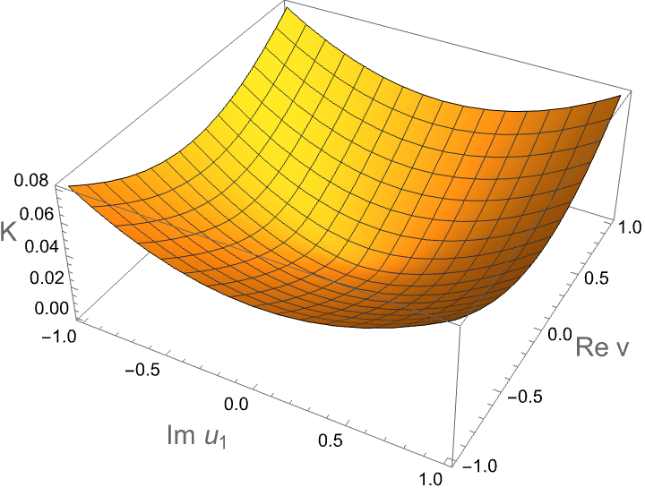
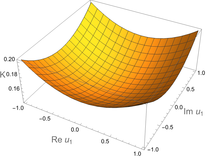
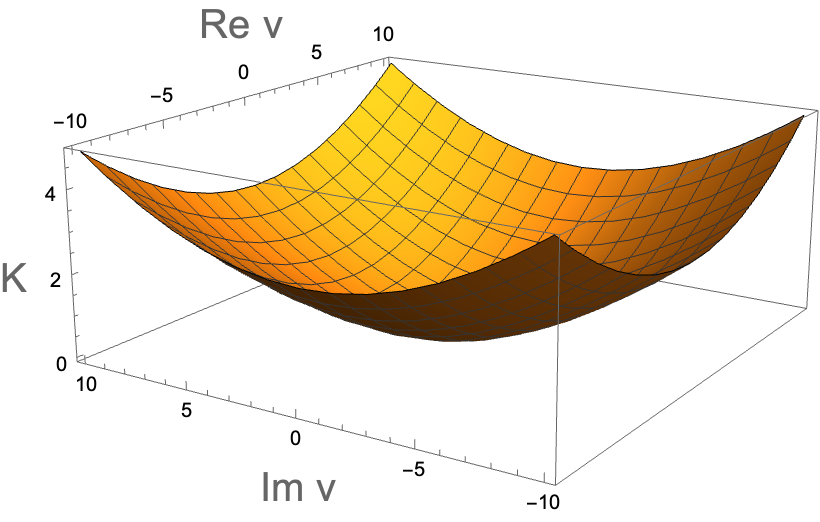
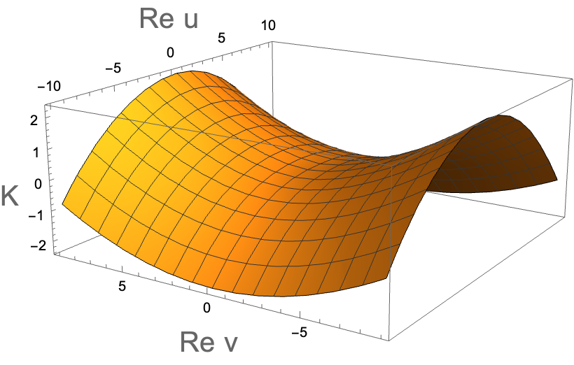
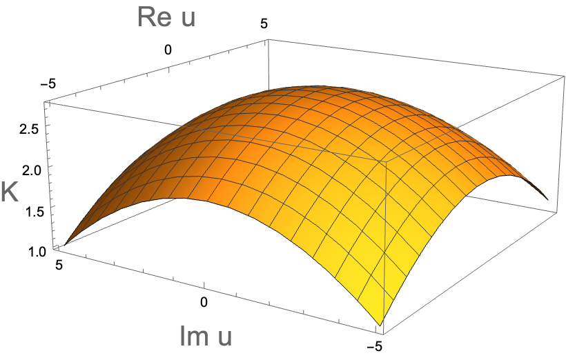
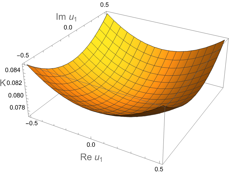
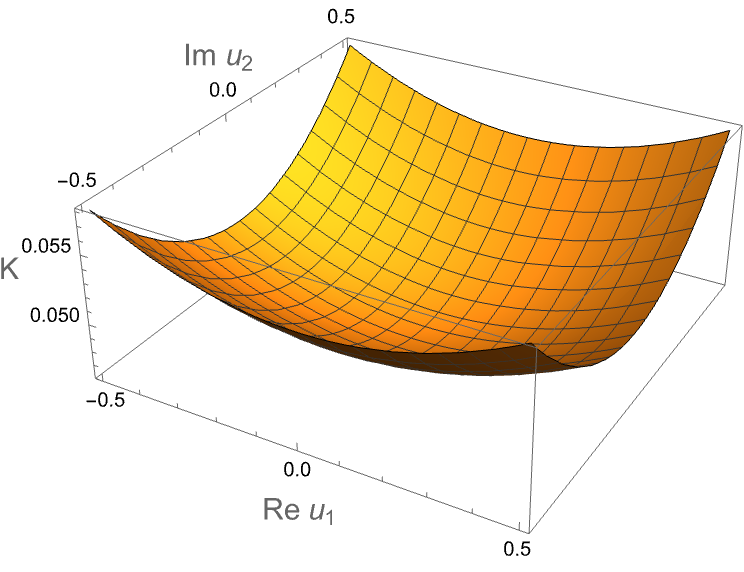
In figure 9 the Kähler potential is plotted in various slices of the intrinsic Coulomb branch moduli $(u,v)$: versus $({\rm Re\,}(v),{\rm Im\,}(v))$ for fixed $u$ in panel (a); versus $({\rm Re\,}(v),{\rm Im\,}(u))$ for fixed ${\rm Re\,}(u),{\rm Im\,}(v)$ in panel (b); and $({\rm Re\,}(u),{\rm Im\,}(u))$ for fixed $v$ in panel (c). One observes in each case that, for the domain plotted, the Kähler potential is manifestly convex. More detailed numerical analysis, not manifestly visible form the plots, establishes that $K_{AB}$ is also positive definite for all values of $u,v$ studied, and vanishes only for $u=v=0$.

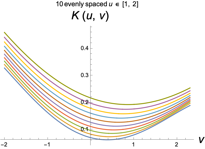
In figure 10 we provide a more detailed numerical analysis of the precise positivity and convexity properties, by taking different representative slicing of the intrinsic moduli space. In panel (a) of figure 10 we set $u=2$, and plot $K_{\text{AD}}$ as a function of $v=e\,e^{i\theta}$ as a function of $r\in[-1,2]$ for a number of discrete values of $\theta$. Convexity and positivity is observed for every such slice. In panel (b) of figure 10 we plot $K_{\text{AD}}$ as a function of real $u\in[-2,2]$ for 10 evenly spaced discrete values of $v\in[1,2]$. Again, we observe positivity and convexity on each slice. Finally, in panel (c) of figure 10 we plot $K_{\text{AD}}$ as a function of real $v\in[-2,2]$ for 10 evenly spaced real values of $u\in[1,2]$, further confirming positivity and convexity.

(a) $v$-plane with $v=re^{i\theta}$

(b) $u$-plane for discrete $v$

(c) $v$-plane for discrete $u$

Figure 10: Plots of $K_{\text{AD}}$ for $(\mathfrak{a}_{1},\mathfrak{a}_{4})$ on discrete slices of the intrinsic moduli space.

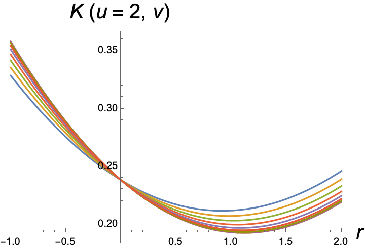
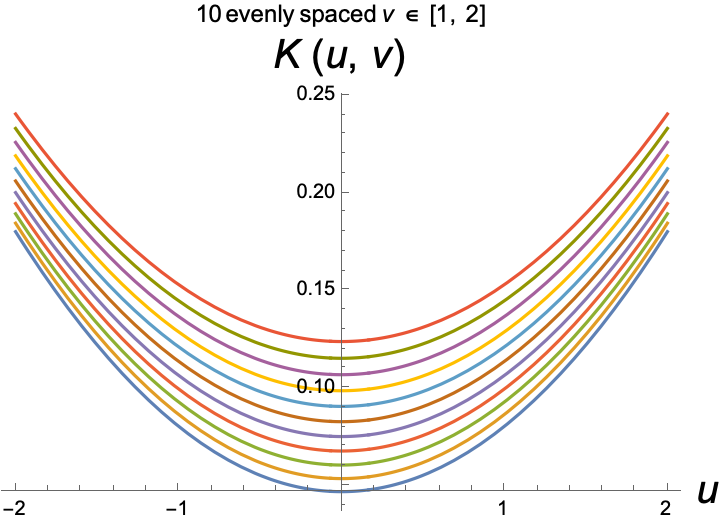
Additional observations include the following. One verifies numerically, for example in panel (b) of figure 10, that the minimum of the Kähler potential over the $u$-plane always occurs at the origin $u=0$ for any $v\not=0$. From panel (c) of figure 10, we also see that for various real (as well as) complex values of $u$, the Kähler potential has a local minimum that is shifted from $v=0$ for any $u\neq 0$, though still respecting positivity and convexity. Finally, the Kähler potential is always positive in all these cases, and the minimum of $K$ is strictly bigger than $0$ if $u\neq 0$.

4.8 A rank-3 example: $(\mathfrak{a}_{1},\mathfrak{a}_{6})$

We consider the dependence of the intrinsic Kähler potential on the three intrinsic moduli $u_{2},u_{1},v$, where the SW curve is given by,

$$\hat{y}^{2}=x^{7}-u_{2}x^{2}-u_{1}x+v$$ (4.36)

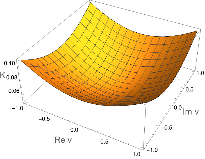
The evaluation of the periods and Kähler potential proceeds very similarly to what we have already described up to rank 2, so we will not go into that here but rather only present the results. We study the regime of fixed $v$, and small $u_{1,2}$ using our expansion. This allows us to produce plots in figure 11 that further support our conjecture that the intrinsic Kähler potential is a convex and positive function with a unique minimum at $K_{\text{AD}}=0$ that is located at the ${\mathbb{Z}}_{7}$-symmetric point.

(a) $u_{1}$-plane

(b) $u_{2}$-plane

(c) $({\rm Re\,}u_{1},{\rm Im\,}u_{2})$-plane

Figure 11: Plots of $K_{\text{AD}}$ for $(\mathfrak{a}_{1},\mathfrak{a}_{6})$ on various slices of the intrinsic moduli space for fixed value of $v$ and different splicings of the intrinsic moduli $u_{1},u_{2}$.

5 Conclusions and future directions

In this paper, we have analyzed three different aspects of Argyres-Douglas (AD) theories, and their embeddings into the moduli-spaces of asymptotically-free gauge theories: the SW periods near the AD points; the marginal stability of mutually local BPS states in a near the AD points; and the intrinsic periods and Kähler potential of $(\mathfrak{a}_{1},\mathfrak{a}_{N-1})$ theories.

5.1 Summary of results

1. For gauge-group ${\text{SU}}(N)$, we evaluated SW periods near the maximal AD points for $N\geq 3$ by a non-trivial analytic continuation of the expansion of the periods obtained near the ${\mathbb{Z}}_{2N}$-symmetric point studied in [15]. Since our expansion is around one or the other maximal AD point, it allows us to access a neighborhood of the maximal AD points that includes the intrinsic Coulomb branch of the AD theory. On regions of overlap, we showed that our expansion has better convergence properties than the expansion considered in [15].

2. For gauge-group ${\text{SU}}(3)$, we revisited the structure of the walls for marginal stability, which were analyzed in [15] only on the restricted slice with $u=0$. Utilizing a combination of our expansion around the ${\mathbb{Z}}_{3}$ point and the numerical integration methods of [15], we mapped out the walls of marginal stability in the 3D space $({\rm Re\,}u,{\rm Im\,}u,\text{Arc})$, where Arc refers to a real-dimension 1 curve in the $v$-plane. This adds a more complete understanding of the walls, and explains the degeneracy-lifting associated with the ${\mathbb{Z}}_{3}$-symmetry of the $v$-plane. We provide partial results for ${\text{SU}}(4)$ on the $u_{2}=u_{1}=0$ slice, and point out some generic features for $N\geq 3$.

3. In the last part of this paper, we explore the intrinsic Coulomb branch of $(\mathfrak{a}_{1},\mathfrak{a}_{N-1})$ theories. We applied the decoupling limit $\Lambda\rightarrow\infty$ to obtain the intrinsic periods and their expansion around the AD point. We then apply this understanding of the periods to exactly compute the intrinsic Kähler potential and prove its positivity and convexity near $v_{n}=0$ on intrinsic slices, except when $4\nmid N$. We numerically test the global positivity and convexity of the Kähler potential over intrinsic slices in a variety of examples up to and including rank-3, i.e. $N=3,4,5,6,7$. We find broad agreement with our analytic results, and find that convexity and positivity are spoiled if we allow non-unitary deformations to be turned on, namely $u_{k\geq\mathfrak{r}}\neq 0$. This is in full agreement with Theorem 4.4.

5.2 Future directions

Let us close this section with some concrete directions for future work.

1. Dynamics of wall-crossing. A key question that we have not addressed in our considerations is whether genuine bound BPS states are formed when we follow a trajectory in the Coulomb branch that crosses a kinematically allowed wall. It would be interesting to explicitly determine the spectrum of BPS states after such a wall is crossed, and determine under what conditions formation of bound BPS states is possible. Work along these lines has been recently undertaken in [33], and it would be interesting to apply these methods to the walls we obtain here. It is worth emphasizing, however, that more complicated phenomena can take place upon wall-crossing that we have also not addressed here – see [32].

2. Integrated correlation functions of the $(\mathfrak{a}_{1},\mathfrak{a}_{N-1})$ stress-tensor. There is a large body of work on integrated correlators in $3d$ ABJM and $4d$ ${\cal N}=4$ super-Yang-Mills [37, 38, 39]. The key motivation behind such work is to provide non-trivial non-perturbative checks of holographic duals in eleven and ten dimensions respectively. Such works often rely on supersymmetric localization, superconformal symmetry, and $S$-duality: all of which can be accessed for AD theories. Recently, holographic duals have been proposed for AD theories in M-theory [40, 41], and it would interesting to compute observables on the field theory side to test these duals. On a related note, there are investigations of the correlators of chiral ring operators in AD theories using supersymmetric localization and the intrinsic SW periods [42].

   In parallel to the work on ${\cal N}=4$ super-Yang-Mills, is there a combination of supersymmetric localization and our expansion of the SW periods that can be used to compute the stress-tensor correlators of AD theories? If yes, what does this correspond to in the proposed holographic dual?

3. SUSY breaking of Argyres-Douglas theories. As was already emphasized explicitly in [20, 14, 15, 21], the convexity of the Kähler potential plays a key role in our understanding of the IR phases of ${\text{SU}}(N)$ adjoint $\text{QCD}_{4}$, which is obtained by deforming pure ${\cal N}=2$ gauge-theory by ${\cal T}_{UV}\sim M^{2}{\rm tr}\bar{\phi}\phi$ near the monopole point. On representation-theoretic grounds, we expect to find a non-supersymmetric interacting CFT if we deform AD theories in an analogous manner [43].

   What can be said about the phases and spectrum of this IR CFT? Can this non-supersymmetric CFT be analyzed by a Lagrangian description obtained by deforming the ${\cal N}=1$ Lagrangian that flows to Argyres-Douglas theory (cf. [44, 45]) in an intermediate step? If such a theory does not admit a Lagrangian realization, can one analyze it using SW theory?

Appendix A Proof of Theorem 2.1

To prove Theorem 2.1 we use the SW differential given in (2.18) and the definition of the integrals $R(\zeta)$ in (2.19). Substituting the multinomial expansion for $V(z)^{M}$ in powers of $z$,

$$V(z)^{M} =\sum_{\ell_{1},\cdots,\ell_{N-2}=0}^{M}\binom{M}{\ell_{1},\cdots,\ell_{N-2}}\,v_{1}^{\ell_{1}}\cdots v_{N-2}^{\ell_{N-2}}\,z^{L-1}$$ (A.1)

where we use the combinations $L$ and $M$ familiar from (2.10), gives the following expansion of the SW differential,

$$\lambda = {v^{{1\over 2}+\frac{1}{N}}\over\sqrt{-2}}\sum_{k=0}^{\infty}{\Gamma(k+{1\over 2})\over\Gamma({1\over 2})\,k!}\,\left({v\over 2}\right)^{k}\sum_{{\ell_{n}=0\atop n=1,\cdots,N-2}}^{\infty}{\Gamma({1\over 2}-k+M)\over\Gamma({1\over 2}-k)}{v_{1}^{\ell_{1}}\cdots v_{N-2}^{\ell_{N-2}}\over\ell_{1}!\cdots\ell_{N-2}!}$$ (A.2)

$$\hskip 36.135pt\times\left(Nz^{N}-\sum_{n=1}^{N-2}nv_{n}z^{n}\right){z^{L-1}dz\over\big{(}z^{N}+1\big{)}^{{1\over 2}-k+M}}$$

The integral over $z$ from 0 to $\zeta$ greatly simplifies for $\zeta^{N}=-1$ and we obtain,

$$\int_{0}^{\zeta}{z^{\gamma-1}\,dz\over(z^{N}+1)^{p}}={\xi^{\gamma}\over\gamma}F(p,\tfrac{\gamma}{N};1+\tfrac{\gamma}{N};1)={\xi^{\gamma}\over N}{\Gamma(\tfrac{\gamma}{N})\Gamma(1-p)\over\Gamma(1+\tfrac{\gamma}{N}-p)}$$ (A.3)

The integrals of $\lambda$ given by the expansion in (A.2) correspond to the values $p={\tfrac{1}{2}}-k+M$, and $\gamma=L+N$ or $\gamma=L+n$. As a result, we obtain,

$$i\pi R(\xi) = {v^{{1\over 2}+\frac{1}{N}}\over\sqrt{-2}}\sum_{k=0}^{\infty}{(-)^{M}}{\Gamma(k+{1\over 2})^{2}\over\Gamma({1\over 2})\,k!}\,\left({v\over 2}\right)^{k}\sum_{{\ell_{n}=0\atop n=1,\cdots,N-2}}^{\infty}{v_{1}^{\ell_{1}}\cdots v_{N-2}^{\ell_{N-2}}\over\ell_{1}!\cdots\ell_{N-2}!}$$ (A.4)

$$\times\bigg{(}{\xi^{L+N}\,\Gamma(1+\tfrac{L}{N})\over\Gamma(\frac{3}{2}+\tfrac{L}{N}+k-M)}-\sum_{n=1}^{N-2}{n\over N}\,v_{n}\,{\xi^{n+L}\,\Gamma(\tfrac{n+L}{N})\over\Gamma({1\over 2}+\tfrac{n+L}{N}+k-M)}\bigg{)},$$

where we have made use of the reflection formula for $\Gamma$-function $\Gamma(z)\Gamma(1-z)\sin(\pi z)=\pi$. The term labelled by $n$ under the finite sum over $n$ in the second line corresponds to shifting $\ell_{n}\to\ell_{n}-1$ and adding these contributions simplifies the sum as follows,

$$i\pi R(\xi)={v^{{1\over 2}+\frac{1}{N}}\over\sqrt{-2\pi}N}\sum_{{\ell_{n}=0\atop n=1,\cdots,N-2}}^{\infty}\!\!\!\!(-)^{M}\xi^{L}{v_{1}^{\ell_{1}}\cdots v_{N-2}^{\ell_{N-2}}\over\ell_{1}!\cdots\ell_{N-2}!}\sum_{k=0}^{\infty}{\Gamma(k+{1\over 2})^{2}\,\Gamma(\tfrac{L}{N})\over\Gamma(\frac{3}{2}+\tfrac{L}{N}+k-M)\,k!}\,\left({v\over 2}\right)^{k}\quad$$ (A.5)

Relabelling $k\to\ell_{0}$, $v\to v_{0}$ and choosing the branch $\sqrt{-2\pi}=i\sqrt{2\pi}$ produces formula (2.22) and thereby completes the proof of Theorem 2.1.

Appendix B Convergence, long periods, and elliptic form for ${\text{SU}}(3)$

We explicitly display the coefficients of the ${\mathbb{Z}}_{3}$ expansion in this appendix, and examine the convergence criterion for the ${\text{SU}}(3)$ series. Then we demonstrate that an appropriate choice of homology basis makes the long periods analytic.

B.1 The ${\mathbb{Z}}_{6}$ expansion

Explicit formulas for the periods in the case $N=3$ were obtained in [7] using Picard-Fuchs equations. The authors expressed their results in terms of Appell $F_{4}$ functions [46, 22], which can be defined by the following series expansion,

$$F_{4}(a,b,c_{1},c_{2};x,y)=\sum_{m,n=0}^{\infty}{\Gamma(m+n+a)\Gamma(m+n+b)\Gamma(c_{1})\Gamma(c_{2})\over\Gamma(a)\Gamma(b)\Gamma(m+c_{1})\Gamma(n+c_{2}){\,m!\,n!}}\,x^{m}y^{n}$$ (B.1)

The ${\text{SU}}(3)$ periods can be expressed as follows [15],

$$a_{1} =Q(\varepsilon^{1})-Q(\varepsilon^{0}) a_{D,1} =Q(\varepsilon^{2})-Q(\varepsilon^{1})$$

$$a_{2} =Q(\varepsilon^{1})-Q(\varepsilon^{0})+Q(\varepsilon^{3})-Q(\varepsilon^{2}) a_{D,2} =Q(\varepsilon^{4})-Q(\varepsilon^{3})$$ (B.2)

The function $Q(\xi)$ can be expanded in characters of ${\mathbb{Z}}_{6}$

$$Q(\xi) =\sum_{n=0}^{5}\xi^{n}Q_{n} Q_{3} =0$$ (B.3)

The formula for $Q(\xi)$ given in (2.9) may be recast in terms of Appell functions $F_{4}$ expressed as follows in terms of the variables $x=4u_{1}^{3}/27$ and $y=u_{0}^{2}$

$$Q_{1} ={2\pi\over 2^{{1\over 3}}\,3^{{3\over 2}}\,\Gamma(\tfrac{2}{3})^{3}}\,v\,F_{4}(\tfrac{1}{3},\tfrac{1}{3},\tfrac{2}{3},\tfrac{3}{2};x,y) Q_{2} ={2\pi\over 2^{{1\over 3}}\,3^{2}\,\Gamma(\tfrac{2}{3})^{3}}\,u\,F_{4}(\tfrac{1}{6},\tfrac{1}{6},\tfrac{4}{3},\tfrac{1}{2};x,y)$$

$$Q_{4} ={2^{{1\over 3}}\,3^{{3\over 2}}\,\Gamma(\tfrac{2}{3})^{3}\over 4\pi^{2}}\,F_{4}(-\tfrac{1}{6},-\tfrac{1}{6},\tfrac{2}{3},\tfrac{1}{2};x,y) Q_{5} ={2^{{1\over 3}}\,\Gamma(\tfrac{2}{3})^{3}\over 4\pi^{2}}\,uv\,F_{4}(\tfrac{2}{3},\tfrac{2}{3},\tfrac{4}{3},\tfrac{3}{2};x,y)$$ (B.4)

Additionally, $Q_{3}=0$, while $Q_{0}$ cancels out of all periods. Note that the double infinite series for the Appell function is absolutely convergent for $\sqrt{|x|}+\sqrt{|y|}<1$ which gives the following region of absolute convergence in terms of $u$ and $v$,

$$\tfrac{2}{\sqrt{27}}\,|u|^{{3\over 2}}+|v|<1\,.$$ (B.5)

Beyond this region, partial analytic continuation formulas are known for $F_{4}$,

$$F_{4}(a,b,c_{1},c_{2};x,y) ={\Gamma(c_{1})\Gamma(b-a)\over\Gamma(b)\Gamma(c_{1}-a)}\,(-x)^{-a}F_{4}(a,a+1-c_{1},a+1-b,c_{2};\tfrac{1}{x},\tfrac{y}{x})$$ (B.7)

$$\ +{\Gamma(c_{1})\Gamma(a-b)\over\Gamma(a)\Gamma(c_{1}-b)}\,(-x)^{-b}F_{4}(b,b+1-c_{1},b+1-a,c_{2};\tfrac{1}{x},\tfrac{y}{x})\qquad$$

which gives the following region in terms of $u_{1}$ and $u_{0}$,

$$1+|u_{0}|<\tfrac{2}{\sqrt{27}}\,|u_{1}|^{{3\over 2}}$$ (B.8)

allowing us to explore the region of large $|u_{1}|$ and small $|u_{0}|$. Recent progress on the analytic continuation of $F_{4}$ may be found in [47].

B.2 The ${\mathbb{Z}}_{6}$ decomposition from the ${\mathbb{Z}}_{3}$ expansion

The above-mentioned decomposition in terms of the characters of ${\mathbb{Z}}_{6}$ reduces to

$$Q(\xi) =(Q_{0}+Q_{3})\xi^{0}+(Q_{1}+Q_{4})\xi^{1}+(Q_{2}+Q_{5})\xi^{2}\qquad\text{ for }\xi^{3}=+1$$

$$Q(\xi) =(Q_{0}-Q_{3})\xi^{0}+(Q_{1}-Q_{4})\xi^{1}+(Q_{2}-Q_{5})\xi^{2}\qquad\text{ for }\xi^{3}=-1$$ (B.9)

These coefficients may be extracted from the expression for $Q(\xi)$ in (2.42) by parametrizing $m=3\mu+\nu$ where $\nu=0,1,2$ and $\mu\geq 0$.

• For $\xi^{3}=-1$ we obtain,

  $$Q_{0}-Q_{3} = {u^{2}\,v^{-{1\over 2}}\over 3\sqrt{2}\,\pi}\sum_{\mu=0}^{\infty}{\mu!\,\Gamma({1\over 2})\over\Gamma({\tfrac{1}{2}}-2\mu)\,(3\mu+2)!}\,F({\tfrac{1}{2}},{\tfrac{1}{2}};{\tfrac{1}{2}}-2\mu;\tfrac{v}{2})\left({u^{3}\over v^{2}}\right)^{\mu}$$

  $$Q_{1}-Q_{4} = -{v^{\frac{5}{6}}\over 3\sqrt{2}\,\pi}\sum_{\mu=0}^{\infty}{\Gamma(\tfrac{1}{3}+\mu)\Gamma({1\over 2})\over\Gamma(\tfrac{11}{6}-2\mu)\,(3\mu)!}\,F({\tfrac{1}{2}},{\tfrac{1}{2}};\tfrac{11}{6}-2\mu;\tfrac{v}{2})\left({u^{3}\over v^{2}}\right)^{\mu}$$

  $$Q_{2}-Q_{5} = {u\,v^{\frac{1}{6}}\over 3\sqrt{2}\,\pi}\sum_{\mu=0}^{\infty}{\Gamma(\tfrac{2}{3}+\mu)\Gamma({1\over 2})\over\Gamma(\tfrac{7}{6}-2\mu)\,(3\mu+1)!}\,F({\tfrac{1}{2}},{\tfrac{1}{2}};\tfrac{7}{6}-2\mu;\tfrac{v}{2})\left({u^{3}\over v^{2}}\right)^{\mu}$$ (B.10)

• For $\xi^{3}=1$ we obtain,

  $$Q_{0}+Q_{3} = {u^{2}\ v^{-{1\over 2}}\over 3\sqrt{2}\,\pi}\sum_{\mu=0}^{\infty}{\mu!\,\Gamma({1\over 2}+2\mu)\over\Gamma({1\over 2})(3\mu+2)!}F({\tfrac{1}{2}},{\tfrac{1}{2}};{\tfrac{1}{2}}-2\mu;\tfrac{v}{2})\left({u^{3}\over v^{2}}\right)^{\mu}$$ (B.11)

  $$Q_{1}+Q_{4} = \sum_{\mu=0}^{\infty}{\Gamma(\tfrac{1}{3}+\mu)\over(3\mu)!}\bigg{[}{v^{\frac{5}{6}}\over 3\sqrt{2}\,\pi}\,{\Gamma(-\frac{5}{6}+2\mu)\over\Gamma({1\over 2})}F({\tfrac{1}{2}},{\tfrac{1}{2}};\tfrac{11}{6}-2\mu;\tfrac{v}{2})\left({u^{3}\over v^{2}}\right)^{\mu}$$

  $$\hskip 79.49744pt{+}{2^{2/3}\Gamma({1\over 2})\Gamma(\frac{5}{6}-2\mu)\,(4u^{3})^{\mu}\over 6\,\Gamma(\frac{2}{3}-\mu)^{2}\Gamma(\frac{7}{6}-\mu)^{2}}F(2\mu-\tfrac{1}{3},2\mu-\tfrac{1}{3};\tfrac{1}{6}+2\mu;\tfrac{v}{2})\bigg{]}$$

  $$Q_{2}+Q_{5} = u\sum_{\mu=0}^{\infty}{\Gamma(\tfrac{2}{3}+\mu)\over(3\mu+1)!}\bigg{[}2^{1/3}{\Gamma(-\frac{1}{6}+2\mu)\,(4u^{3})^{\mu}\over 6\,\Gamma({1\over 2})^{3}}(2v)^{\frac{1}{6}-2\mu}F({\tfrac{1}{2}},{\tfrac{1}{2}};\tfrac{7}{6}-2\mu;\tfrac{v}{2})$$

  $$\hskip 79.49744pt{+}{2^{4/3}\Gamma({1\over 2})\Gamma(\frac{1}{6}-2\mu)\,(4u^{3})^{\mu}\over 6\,\Gamma(\frac{1}{3}-\mu)^{2}\Gamma(\frac{5}{6}-\mu)^{2}}F(\tfrac{1}{3}+2\mu,\tfrac{1}{3}+2\mu;\tfrac{5}{6}+2\mu;\tfrac{v}{2})\bigg{]}$$

Using the reflection formula, $Q_{0}+Q_{3}=Q_{0}-Q_{3}$ so that $Q_{3}=0$, consistent with [15].

B.3 Convergence of the ${\mathbb{Z}}_{3}$ series

To study the convergence properties of the series for $Q(\xi)$ when $\xi^{3}=-1$ we use the reflection and multiplication formulas for $\Gamma$-functions to obtain,

$$Q(\xi) = {v^{\frac{5}{6}}\over 3\pi}\sum_{\nu=0,1,2}(-)^{\nu+1}\xi^{\nu+1}\sin\pi(\tfrac{4\nu-5}{6}){\cal Q}_{\nu}$$

$${\cal Q}_{\nu} = {1\over 2^{\frac{4}{3}}3^{1\over 2}}\sum_{\mu=0}^{\infty}{\Gamma(\mu+\frac{4\nu-5}{12})\Gamma(\mu+\frac{4\nu+1}{12})\over\Gamma(\mu+\frac{\nu+2}{3})\Gamma(\mu+\frac{\nu+3}{3})}\,F({\tfrac{1}{2}},{\tfrac{1}{2}};\tfrac{11-4\nu}{6}-2\mu;\tfrac{v}{2})\left({4u^{3}\over 27v^{2}}\right)^{\mu+\frac{\nu}{3}}$$ (B.1)

We begin by considering the $\lambda\to+\infty$ behavior of the hypergeometric function which is given by the following Taylor series for fixed value of $|z|<1$,

$$F({\tfrac{1}{2}},{\tfrac{1}{2}};\lambda;z)=\sum_{k=0}^{\infty}{\Gamma(k+{1\over 2})^{2}\,\Gamma(\lambda)\over\Gamma({1\over 2})^{2}\,\Gamma(k+\lambda)\,k!}\,z^{k}$$ (B.2)

The first few terms are given by,

$$F({\tfrac{1}{2}},{\tfrac{1}{2}};\lambda;z)=1+{z\over 4\lambda}+{9\,z^{2}\over 32\,\lambda(\lambda+1)}+{75\,z^{3}\over 128\,\lambda(\lambda+1)(\lambda+2)}+{\cal O}(z^{4})$$ (B.3)

The series is absolutely convergent for any compact subset of the open disc $|z|<1$ uniformly in $\lambda$ greater than any fixed number strictly greater than one; for our purposes it suffices to choose $\lambda\geq 1$. For fixed $|z|<1$, the absolute value of each term in the series strictly decreasing as $\lambda\to+\infty$ and therefore the limit of the series as $\lambda\to+\infty$ is simply given by,

$$\lim_{\lambda\to+\infty}F({\tfrac{1}{2}},{\tfrac{1}{2}};\lambda;z)=1\qquad\hbox{ for all }\quad|z|<1$$ (B.4)

Next, we consider the case where $\lambda\to-\lambda$ in the hypergeometric function, and use the general formula below to relate this case to the previous one,

$$F(a,b;-\lambda;z) = {z^{\lambda+1}\Gamma(-\lambda)\Gamma(a+1+\lambda)\Gamma(b+1+\lambda)\over(1-z)^{\lambda+a+b}\Gamma(a)\Gamma(b)\Gamma(\lambda+2)}F(1-a,1-b;\lambda+2;z)$$ (B.5)

$$+{\Gamma(a+1+\lambda)\Gamma(b+1+\lambda)\over\Gamma(a+b+1+\lambda)\Gamma(\lambda+1)}F(a,b;a+b+1+\lambda;1-z)$$

For the special case $a=b={\tfrac{1}{2}}$ of interest here, we have the following simplification,

$$F({\tfrac{1}{2}},{\tfrac{1}{2}};-\lambda;z) = -{z^{\lambda+1}\over(1-z)^{\lambda+1}}{\Gamma(-1-\lambda)\Gamma(\frac{3}{2}+\lambda)^{2}\over\Gamma({1\over 2})^{2}\Gamma(\lambda+1)}F({\tfrac{1}{2}},{\tfrac{1}{2}};\lambda+2;z)$$ (B.6)

$$+{\Gamma(\tfrac{3}{2}+\lambda)^{2}\over\Gamma(\lambda+2)\Gamma(\lambda+1)}F({\tfrac{1}{2}},{\tfrac{1}{2}};\lambda+2;1-z)$$

For the first term to admit a finite limit as $\lambda\to+\infty$, we must require $|z|<|1-z|$, in which case the contribution from the first term tends to zero. That this sufficient condition is also necessary may be established numerically by taking the limit $z\to{1\over 2}$ and verifying that the limit to be established below does not hold. In the absence of the first term, the limit of the second term is then given by,

$$F({\tfrac{1}{2}},{\tfrac{1}{2}};-\lambda;z)={\Gamma(\tfrac{3}{2}+\lambda)^{2}\over\Gamma(\lambda+2)\Gamma(\lambda+1)}\left(1+{1-z\over 4\lambda}+{\cal O}(\lambda^{-2})\right)$$ (B.7)

and thus,

$$\lim_{\lambda\to+\infty}F({\tfrac{1}{2}},{\tfrac{1}{2}};-\lambda;z)=1\qquad\hbox{ for all }\quad|z|<\hbox{min}(1,|1-z|)$$ (B.8)

Convergence of the series for ${\cal Q}_{\nu}$

We shall now use the results of the preceding subsection to investigate the convergence properties of the series given in (B.1) for ${\cal Q}_{\nu}$. The large $\mu$ behavior of the prefactor of $\Gamma$-functions is as follows,

$${\Gamma(\mu+\frac{4\nu-5}{12})\Gamma(\mu+\frac{4\nu+1}{12})\over\Gamma(\mu+\frac{\nu+2}{3})\Gamma(\mu+\frac{\nu+3}{3})}={1\over\mu^{2}}\left(1+{\cal O}(\lambda^{-1})\right)$$ (B.9)

In view of the asymptotics of the hypergeometric function for $\mu\to\infty$ in the domain,

$$|\tfrac{v}{2}|<{\tfrac{1}{2}}\hskip 72.26999pt|\tfrac{v}{2}|<|1-\tfrac{v}{2}|$$ (B.10)

the large $\mu$ behavior of the summand in ${\cal Q}_{\nu}$ is as follows,

$${1\over\mu^{2}}\left({4u^{3}\over 27v^{2}}\right)^{\mu+\frac{\nu}{3}}$$ (B.11)

and the series is convergent provided,

$$\left|{4u^{3}\over 27}\right|<|v|^{2}=|1-u_{0}|^{2}<1$$ (B.12)

since the condition $|\tfrac{v}{2}|<{\tfrac{1}{2}}$ implies the condition $|\tfrac{v}{2}|<|1-\tfrac{v}{2}|$.

B.4 Elliptic expression for the $(\mathfrak{a}_{1},\mathfrak{a}_{2})$ Kähler potential

For completeness, we add here the exact expression for the intrinsic periods in terms of the elliptic formulation developed in subsection 2.4.3. The SW differential is given by,

$$\lambda=-i\frac{dz}{2\sqrt{2}(2\omega)^{5}}\left(12\wp(z)^{3}-g_{2}\wp(z)\right),$$ (B.13)

Using the homology basis of subsection 2.4.3, $\mathfrak{A}=[0,2\pi i],\mathfrak{B}=[0,2\pi i\tau]$, the SW periods may be read off from Theorem 2.6 by setting $k=\ell=m=0$, and we have,

$$a =-i\,\frac{{\sf E}_{2}{\sf E}_{4}-{\sf E}_{6}}{720\sqrt{2\pi}(2\omega)^{5}} a_{D}-\tau a =\frac{-{\sf E}_{4}}{60(2\pi)^{\frac{3}{2}}(2\omega)^{5}}$$ (B.14)

The right formula confirms that $a_{D}=\rho a$ for the AD theory since ${\sf E}_{4}(\rho)=0$. As one approaches the AD point, $u,v\to 0$, which forces $\omega\to\infty$ since ${\sf E}_{6}(\rho)$ is non-vanishing. Thus, both periods tend to zero at the AD point, as expected. The Kähler potential is given by,

$$K_{\text{AD}}=\frac{{\rm Im\,}(\tau)}{2\pi}|a|^{2}-{{\rm Re\,}\big{(}\bar{\sf E}_{4}({\sf E}_{2}{\sf E}_{4}-{\sf E}_{6})\big{)}\over 675\,\pi^{3}|4\omega|^{10}}$$ (B.15)

One verifies that upon setting $\tau=\rho$ and then letting $\omega\rightarrow\infty$, the intrinsic Kähler potential $K_{\text{AD}}$ tends to zero as expected.

References

- [1] N. Seiberg and E. Witten, “Electric - magnetic duality, monopole condensation, and confinement in N=2 supersymmetric Yang-Mills theory,” Nucl. Phys. B 426, 19-52 (1994) [erratum: Nucl. Phys. B 430, 485-486 (1994)] arXiv:hep-th/9407087.
- [2] N. Seiberg and E. Witten, “Monopoles, duality and chiral symmetry breaking in N=2 supersymmetric QCD,” Nucl. Phys. B 431, 484-550 (1994) arXiv:hep-th/9408099.
- [3] A. Klemm, W. Lerche, S. Theisen, S. Yankielowicz, “Simple Singularities and N=2 Supersymmetric Yang-Mills Theory,” Nucl. Phys. B 431, 484-550 (1994) arXiv:hep-th/9408099.
- [4] P. C. Argyres and A. E. Faraggi, “The vacuum structure and spectrum of N=2 supersymmetric SU(n) gauge theory,” Phys. Rev. Lett. 74, 3931-3934 (1995) arXiv:hep-th/9411057.
- [5] A. Hanany and Y. Oz, “On the quantum moduli space of vacua of N=2 supersymmetric SU(N(c)) gauge theories,” Nucl. Phys. B 452, 283-312 (1995) arXiv:hep-th/9505075.
- [6] P. C. Argyres, M. R. Plesser and A. D. Shapere, “The Coulomb phase of N=2 supersymmetric QCD,” Phys. Rev. Lett. 75, 1699-1702 (1995) arXiv:hep-th/9505100.
- [7] A. Klemm, W. Lerche and S. Theisen, “Nonperturbative effective actions of N=2 supersymmetric gauge theories,” Int. J. Mod. Phys. A 11, 1929-1974 (1996) arXiv:hep-th/9505150.
- [8] K. A. Intriligator and N. Seiberg, “Lectures on supersymmetric gauge theories and electric-magnetic duality,” Nucl. Phys. B Proc. Suppl. 45BC, 1-28 (1996) arXiv:hep-th/9509066.
- [9] E. D’Hoker, I. M. Krichever and D. H. Phong, “The Effective prepotential of N=2 supersymmetric SU(N(c)) gauge theories,” Nucl. Phys. B 489, 179-210 (1997) arXiv:hep-th/9609041.
- [10] Y. Tachikawa, “N=2 supersymmetric dynamics for pedestrians,” arXiv:1312.2684.
- [11] M. Martone, “The constraining power of Coulomb Branch Geometry: lectures on Seiberg-Witten theory,” arXiv:2006.14038.
- [12] M. R. Douglas and S. H. Shenker, “Dynamics of SU(N) supersymmetric gauge theory,” Nucl. Phys. B 447, 271-296 (1995) arXiv:hep-th/9503163.
- [13] E. D’Hoker and D. H. Phong, “Strong coupling expansions of SU(N) Seiberg-Witten theory,” Phys. Lett. B 397, 94-103 (1997) arXiv:hep-th/9701055.
- [14] E. D’Hoker, T. T. Dumitrescu, E. Gerchkovitz and E. Nardoni, “Revisiting the multi-monopole point of SU(N) = 2 gauge theory in four dimensions,” JHEP 09, 003 (2021) arXiv:2012.11843.
- [15] E. D’Hoker, T. T. Dumitrescu and E. Nardoni, “Exploring the strong-coupling region of SU(N) Seiberg-Witten theory,” JHEP 11, 102 (2022) arXiv:2208.11502.
- [16] P. C. Argyres and M. R. Douglas, “New phenomena in SU(3) supersymmetric gauge theory,” Nucl. Phys. B 448, 93-126 (1995) arXiv:hep-th/9505062.
- [17] F. Ferrari and A. Bilal, “The Strong coupling spectrum of the Seiberg-Witten theory,” Nucl. Phys. B 469, 387-402 (1996) arXiv:hep-th/9602082.
- [18] A. Bilal and F. Ferrari, “Curves of marginal stability, and weak and strong coupling BPS spectra in N=2 supersymmetric QCD,” Nucl. Phys. B 480, 589-622 (1996) arXiv:hep-th/9605101.
- [19] A. Bilal and F. Ferrari, “The BPS spectra and superconformal points in massive N=2 supersymmetric QCD,” Nucl. Phys. B 516, 175-228 (1998) arXiv:hep-th/9706145.
- [20] C. Córdova and T. T. Dumitrescu, “Candidate Phases for SU(2) Adjoint QCD4 with Two Flavors from Supersymmetric Yang-Mills Theory,” arXiv:1806.09592.
- [21] E. D’Hoker, T. T. Dumitrescu, E. Gerchkovitz and E. Nardoni, to appear.
- [22] A. Erdelyi editor, Bateman Manuscript project, Higher transcendental Functions, Vol I, Chapter V, Robert E. Krieger Publishing Company, 1981.
- [23] D. Gaiotto, “N=2 dualities,” JHEP 08, 034 (2012) arXiv:0904.2715.
- [24] P. Argyres, M. Lotito, Y. Lü and M. Martone, “Geometric constraints on the space of = 2 SCFTs. Part I: physical constraints on relevant deformations,” JHEP 02, 001 (2018) arXiv:1505.04814.
- [25] P. C. Argyres, M. Lotito, Y. Lü and M. Martone, “Geometric constraints on the space of = 2 SCFTs. Part II: construction of special Kähler geometries and RG flows,” JHEP 02, 002 (2018) arXiv:1601.00011.
- [26] P. C. Argyres, M. Lotito, Y. Lü and M. Martone, “Expanding the landscape of = 2 rank 1 SCFTs,” JHEP 05, 088 (2016) arXiv:1602.02764.
- [27] P. Argyres, M. Lotito, Y. Lü and M. Martone, “Geometric constraints on the space of = 2 SCFTs. Part III: enhanced Coulomb branches and central charges,” JHEP 02, 003 (2018) arXiv:1609.04404.
- [28] P. C. Argyres and M. Martone, “Scaling dimensions of Coulomb branch operators of 4d N=2 superconformal field theories,” arXiv:1801.06554.
- [29] J. Kaidi, M. Martone, L. Rastelli and M. Weaver, “Needles in a haystack. An algorithmic approach to the classification of 4d = 2 SCFTs,” JHEP 03, 210 (2022) arXiv:2202.06959.
- [30] E. D’Hoker and J. Kaidi, “Lectures on modular forms and strings,” arXiv:2208.07242.
- [31] M. Alim, S. Cecotti, C. Cordova, S. Espahbodi, A. Rastogi and C. Vafa, “ quantum field theories and their BPS quivers,” Adv. Theor. Math. Phys. 18, no.1, 27-127 (2014) arXiv:1112.3984.
- [32] D. Gaiotto, G. W. Moore and A. Neitzke, “Wall-crossing, Hitchin systems, and the WKB approximation,” Adv. Math. 234, 239-403 (2013) arXiv:0907.3987.
- [33] M. Alim, F. Beck, A. Biggs and D. Bryan, “Special geometry, quasi-modularity and attractor flow for BPS structures,” [arXiv:2308.16854 [hep-th]].
- [34] S. Cecotti, A. Neitzke and C. Vafa, “R-Twisting and 4d/2d Correspondences,” arXiv:1006.3435.
- [35] S. Cecotti and C. Vafa, “Classification of complete N=2 supersymmetric theories in 4 dimensions,” arXiv:1103.5832.
- [36] T. Eguchi and K. Hori, “N=2 superconformal field theories in four-dimensions and A-D-E classification,” arXiv:hep-th/9607125.
- [37] D. J. Binder, S. M. Chester, S. S. Pufu and Y. Wang, “ = 4 Super-Yang-Mills correlators at strong coupling from string theory and localization,” JHEP 12, 119 (2019) arXiv:1902.06263.
- [38] S. M. Chester, M. B. Green, S. S. Pufu, Y. Wang and C. Wen, “Modular invariance in superstring theory from = 4 super-Yang-Mills,” JHEP 11, 016 (2020) arXiv:1912.13365.
- [39] S. M. Chester, M. B. Green, S. S. Pufu, Y. Wang and C. Wen, “New modular invariants in = 4 Super-Yang-Mills theory,” JHEP 04, 212 (2021) arXiv:2008.02713.
- [40] I. Bah, F. Bonetti, R. Minasian and E. Nardoni, “Holographic Duals of Argyres-Douglas Theories,” Phys. Rev. Lett. 127, no.21, 211601 (2021) arXiv:2105.11567.
- [41] I. Bah, F. Bonetti, R. Minasian and E. Nardoni, “M5-brane sources, holography, and Argyres-Douglas theories,” JHEP 11, 140 (2021) arXiv:2106.01322.
- [42] A. Bissi, F. Fucito, A. Manenti, J. F. Morales and R. Savelli, “OPE coefficients in Argyres-Douglas theories,” JHEP 06, 085 (2022) arXiv:2112.11899.
- [43] D. Xie, “Soft supersymmetry breaking of 4d SCFT,” arXiv:1905.00345.
- [44] K. Maruyoshi and J. Song, “ deformations and RG flows of SCFTs,” JHEP 02, 075 (2017) arXiv:1607.04281.
- [45] K. Maruyoshi and J. Song, “Enhancement of Supersymmetry via Renormalization Group Flow and the Superconformal Index,” Phys. Rev. Lett. 118, no.15, 151602 (2017) arXiv:1606.05632.
- [46] P. Appell and J. Kampé de Fériet, Fonctions Hyper-géometriques and Hyper-sphériques - Polynomes d’Hermite, Gauthier-Villars, Paris (1929);
- [47] B. Ananthanarayan, S. Friot, S. Ghosh and A. Hurier, “New analytic continuations for the Appell series from quadratic transformations of the Gauss function,” arXiv:2005.07170.
- [48] N.M. Temme, “Large parameter cases of the Gauss hypergeometric function”, Journal of Computational and Applied Mathematics 153 (2003) 441-462.