Orbital Polarimetric Tomography of a Flare Near the Sagittarius A^∗ Supermassive Black Hole

Abstract

The interaction between the supermassive black hole at the center of the Milky Way, Sagittarius A^∗, and its accretion disk, occasionally produces high energy flares seen in X-ray, infrared and radio. One mechanism for observed flares is the formation of compact bright regions that appear within the accretion disk and close to the event horizon. Understanding these flares can provide a window into black hole accretion processes. Although sophisticated simulations predict the formation of these flares, their structure has yet to be recovered by observations. Here we show the first three-dimensional (3D) reconstruction of an emission flare in orbit recovered from ALMA light curves observed on April 11, 2017. Our recovery results show compact bright regions at a distance of roughly 6 times the event horizon. Moreover, our recovery suggests a clockwise rotation in a low-inclination orbital plane, a result consistent with prior studies by EHT and GRAVITY collaborations. To recover this emission structure we solve a highly ill-posed tomography problem by integrating a neural 3D representation (an emergent artificial intelligence approach for 3D reconstruction) with a gravitational model for black holes. Although the recovered 3D structure is subject, and sometimes sensitive, to the model assumptions, under physically motivated choices we find that our results are stable and our approach is successful on simulated data. We anticipate that in the future, this approach could be used to analyze a richer collection of time-series data that could shed light on the mechanisms governing black hole and plasma dynamics.

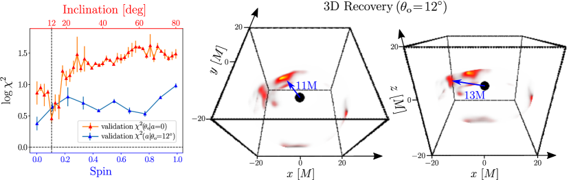
Figure 1: [Left panel] The validation $\chi^{2}$ indicates a preference toward low inclination angles (red curve) $\theta_{\rm o}<18^{\circ}$ with a local minimum around $\theta_{\rm o}=12^{\circ}$. This preference towards low inclination is also apparent in the data fits (analysis in Supplementary Material). Furthermore, our analysis is largely insensitive to the black hole spin. [Right panels] A recovered 3D volume visualized from two view angles in intrinsic (flat space) coordinates (the event horizon illustrated for size comparison). The recovery shows two emission regions (blue arrows) at radii of $\sim 11/13{\rm M}^{\ref{footnote_M}}$ in a clockwise orbit.

The compact region around the Galactic Center supermassive black hole Sgr A^∗ is a unique environment where the magnetized turbulent flow of an accretion disk is subject to extreme gravitational physics. The dynamical evolution of this complex system occasionally leads to the production of energetic flares [10] seen in X-ray [19], infra-red [8], and radio [27]. The physical nature, structure, origin, formation, and eventual dissipation of flares are topics of active research [17, 8, 15, 2, 26] key to our understanding of accretion flows around black holes. One proposed explanation for Sgr A^∗ flares is the formation of compact bright regions caused by hot pockets of lower-density plasma within the accretion disk, that are rapidly energized (e.g. through magnetic reconnection [1]). These “bubbles”, “hotspots” or “flux tubes”, observed in numerical simulations (e.g. [24]), are hypothesized to form in orbit close to the innermost stable circular orbit (ISCO) of Sgr A^∗. The association of flares with orbiting hotspots close to the event horizon is consistent with near-infrared detections made by the GRAVITY Collaboration [12, 13] and radio observations of the Atacama Large Millimeter/Submillimeter Array (ALMA) [26].

The context for this work is set by the first images [6] of Sgr A^∗ revealed by the Event Horizon Telescope (EHT) collaboration. The images, reconstructed from Very Long Baseline Interferometry (VLBI) observations from April 6–7, 2017, show a ring-like structure with a central brightness depression – a strong suggestion that the source is indeed a supermassive black hole [7]. The presence of synchrotron-radiating matter very close to the horizon of Sgr A^∗ could give rise to complex bright 3D structures that orbit and evolve within the accretion disk. While both [12] and [26] employed a strongly constrained parametric hotspot model (essentially 2D) to interpret their observations, the goal of this work is to step out of the 2D image plane and recover the complex 3D structure of flares as they orbit and evolve in the accretion disk around Sgr A^∗.

We present the first 3D recovery results of a Sgr A^∗ flare from ALMA light curve observations on April 11, 2017 (Fig. 1). In contrast to the quiescent state imaged by EHT on April 6/7 [7], these observations were taken directly after an X-ray flare and exhibit a high degree of variability in radio [4, 27] including distinct coherent patterns in the linearly polarized light curve component [26]. To achieve this 3D reconstruction result we develop a novel computational approach which we term: orbital polarimetric tomography.

Tackling this inverse problem necessitates a change from typical tomography, wherein 3D recovery is enabled by multiple viewpoints. Instead, the tomography setting we propose relies on observing a structure in orbit, traveling through curved spacetime, from a fixed viewpoint. As it orbits the black hole, the emission structure is observed (projected) along different curved ray paths. These observations of the evolving structure over time effectively replace the observations from multiple viewpoints required in traditional tomography. Our approach builds upon prior work on 3D tomography in curved spacetime which showed promising results in simulated future Event Horizon Telescope (EHT) observations [22, 20].

Similar to the computational images recovered by EHT [7] our approach solves an under-constrained inverse problem to fit a model to the data. Nevertheless, ALMA observations do not resolve event horizon scales ($\sim 10^{5}$ lower resolution), which makes the tomography problem we propose particularly challenging. To put it differently, we seek to recover an evolving 3D structure from a single-pixel observation over time. A key advantage for dynamical studies is the very high signal-to-noise and cadence (four seconds) of the ALMA dataset [27], as well as the inclusion of both total intensity and full polarization information [26]. In order to solve this challenging task, we integrate the emerging approach of neural 3D representations [21, 20] with physics constraints. The robustness of the results thus relies on the validity of the constraints imposed by the gravitational and synchrotron emission models.

Our simulation analysis (Supplementary Material) shows how polarimetric light curves contain information that could constrain both the 3D flare structure and inclination angle of Sgr A^∗. While the total intensity light curve is dominated by the accretion disk, such extended emission structures are partially depolarized in an image-average polarization sense [26]. In contrast, compact bright sources, such as a putative hotspot, are characterized by a large fractional linear polarization (LP) and fast evolution on dynamical timescales [14, 26], hence allowing separation of the flare component from the background (accretion).

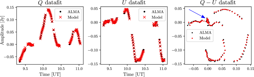
Figure 2: The intrinsic LP curves (centered and de-rotated) and a model fit over a period of $~{}100$ minutes. The model light curves are produced through ray tracing the estimated 3D volume at a fiducial inclination angle of $\theta_{\rm o}=12^{\circ}$ (Fig. 1 analysis). The resulting light curves accurately describe the data including the small looping feature highlighted by the blue arrow (right panel). The data-fit $\chi^{2}\ll 1$ for a noise level of $\sigma_{Q}=\sigma_{U}=0.01~{}\text{Jy}$ [26]

Results

ALMA polarimetric observations of Sgr A^∗

On April 11, 2017, ALMA observed Sgr A^∗ at $\sim 230{\rm GHz}$ as part of a larger EHT campaign. The radio observations directly followed a flare seen in the X-ray (Supplementary Material Fig. 12). The LP, measured by ALMA-only light curves [26, 27] as a complex time series $Q(t)+iU(t)$, appears to evolve in a structured, periodic, manner suggesting a compact emission structure in orbit. The work of [26] hypothesizes a simple bright spot (i.e. idealized point-source [9] or spherical Gaussian [23]) at $r\sim 11{\rm M}$, however, a rigorous data-fitting was not performed. Furthermore, the proposed parametric model is limited and does not explain all of the data features. The orbital polarimetric tomography approach that we propose enables a rigorous data-fitting and recovery of flexible 3D distributions of the emitting matter, relaxing the assumption of a coherent orbiting feature enforced by prior studies [12, 26]. This opens up a new window into understanding the spatial structure and location of flares relative to the event horizon.

Our model, outlined in the Supplementary Material, is able to fit the ALMA light curve data very accurately (see Fig. 2). The optimization procedure simultaneously constrains the inclination angle of the observer and estimates a 3D distribution of the emitting matter associated with this flaring event (Fig. 1), starting from 9:20 UT, about $30$ minutes after the peak of the X-ray flare [26]. Despite the fact that ALMA observations are unresolved (effectively a single pixel with time-dependent complex LP information) at the horizon scale, our analysis suggests some interesting insights:

• Low inclination angles ($\theta_{\rm o}<18^{\circ}$) are preferred by the validation $\chi^{2}$ (Fig. 1 left panel, blue). While the methodology is different, this result is broadly consistent with EHT findings from April 6/7 [8] which favored low inclination angles of $\sim 30^{\circ}$ by comparing recovered images with General Relativistic Magneto Hydro Dynamic simulations. The fiducial model of [26] corresponded to an inclination angle of $\sim 22^{\circ}$. Low inclination was also favored in the analysis of the GRAVITY infra-red flares [12, 13, 14].

• The recovered 3D emission has two compact bright regions at $r\sim 11M,13M$ (Fig. 1 middle/right panels). The location (radius and azimuthal position) of the bright region is consistent with the qualitative analysis of [26].

Data fitting

Before solving the tomography problem, we perform pre-processing according to the procedure outlined in [26]. In particular, we subtract a constant (time-averaged) LP component, interpreted as the ring-like accretion disk component observed by the EHT, and de-rotate the electric vector polarization angle (EVPA) to account for Faraday rotation (details in the Supplementary Material). To obtain a model prediction an initial 3D emission structure is adjusted so that, when placed in orbit, the numerically ray-traced LP light curves align with the observations. Mathematically this is formulated by minimizing a $\chi^{2}$ loss between the observed LP and the model prediction.

Our tomography relies on ray tracing which requires knowledge of the path rays take in 3D curved spacetime. In general, ray paths (geodesics) depend on unknown black hole properties [9]: mass, spin, and inclination. Nevertheless, the mass of Sgr A^∗ is well constrained through stellar dynamics [10]; $M\simeq 4{\times}10^{6}M_{\odot}$ where $M_{\odot}$ denotes solar mass. Furthermore, Fig. 1 illustrates that the loss is not very sensitive to black hole spin: $a\in[0,1]$. Thus, the only remaining unknown is the inclination angle. To estimate the inclination we numerically bin $\theta_{\rm o}\in[0,\pi/2]$ and recover the 3D emission for every given (fixed) angle.

For each inclination angle, we recover a (locally) optimal 3D emission by minimizing a $\chi^{2}$ loss over the model parameters. Practically, for numerical stability, we avoid the extreme angles of face-on and edge-on by gridding $\theta_{\rm o}\in[4^{\circ},80^{\circ}]$ (at $2^{\circ}$ increments). Figure 1 plots a likelihood approximation for $\theta_{\rm o}$, which appears to favor low inclination angles ($\theta_{\rm o}<18^{\circ}$). For each inclination, the recovery is run five times with a random initialization for the 3D structure. Therefore, the error bars are not a measure of posterior uncertainty, rather, they indicate the stability of the locally optimal solution. The 3D structure shown in Fig. 1 is the average structure across all random initialization at an inclination of $\theta_{\rm o}=12^{\circ}$ which corresponds to the $\chi^{2}$ minimum (Fig. 2). In the Appendix, we highlight how the key features of the recovered 3D structure are consistent across a range of inclination angles (within the local minimum basin) and random initialization.

Assumptions and systematic noise

Emission model	Synchrotron fixed vertical magnetic field;    optically thin disk
Dynamical model	Keplerian $t_{0}=$9:20 UT;   clockwise orbit (no radial / vertical velocity);    velocity shear
Gravitational model	Kerr mass $=4.154{\times}10^{6}M_{\odot}$;    non spinning${}^{\ref{footnote_a}}$;    $\theta_{\rm o}$ estimated from data
3D model	Neural representation Recovery domain: $6{\rm M}\leq r\leq 20{\rm M}$ (FOV $\approx 200\mu{\rm as}$);    $|z|\leq 4{\rm M}$

Table 1: This table summarizes the key physical assumptions made. The recovered 3D emission relies on combining the flexibility of 3D neural fields with black-hole physics. Thus, the accuracy of the reconstruction depends on the validity of the model assumptions. In the Supplementary Material we further investigate the effects of some of the assumptions on the data-fit and recovered 3D, including: magnetic field configurations, orbit direction, sub-Keplerian orbits, and the initial time.

The key assumption for orbital tomography is that the 4D (space and time) emission is in orbit around the black hole and can be modeled as a simple transformation to a canonical (or initial) 3D emission. This enables formulating an inverse problem of estimating the 3D emission from observations. While this assumption does not hold in general, it is well suited for compact bright structures over short time scales, during which complex dynamics could be negligible. We consider orbits characterize by a Keplerian angular velocity profile, accounting for shearing due to differential rotation (ignored by the previous analyses [12, 26]) while neglecting the dynamics of cooling, heating, expansion, and turbulence. Furthermore, in modeling synchrotron emission, we assume a (homogeneous) vertical magnetic field, as preferred in the analyses of [12, 26], that is externally fixed and is independent of the flare or accretion disk dynamics. In the Supplementary Material, we examine the effects of other magnetic field configurations (radial, toroidal) and sub-Keplerian orbits on the data-fit and 3D reconstruction. Lastly, we do not model radial (in-fall) or vertical velocity components. We constrain the 3D recovery domain to a region that is best modeled by these assumptions with a radius of $6{\rm M}\leq r\leq 20{\rm M}$ and close to the equatorial disk $|z|\leq 4{\rm M}$ ($6M$ is the innermost stable circular orbit of a non-spinning black hole). Table 1 summarizes the key assumptions made in the reconstruction shown in Fig. 1.

Solving an under-constrained inverse problem requires some form of regularization (whether implicit or explicit). The 3D neural representation has an implicit regularization that favors smooth structures [21, 25] (details in the Supplementary Material). We additionally regularize the recovered total intensity of the flare to be around $0.3~{}\text{Jy}$ [26] with a standard deviation of $0.15~{}\text{Jy}$. The choice to only fit the LP light curves reflects the uncertainty associated with the highly non-polarized intensity of the background accretion disk. In the Supplementary Material, we quantitatively assess the effect of the background accretion disk on simulated reconstruction results.

Although the evolution of the recovered 3D structure well matches the observed light curve, there could be alternative morphologies and orbital models that also match the data. This non-uniqueness of the solution is a general feature of under-constrained inverse problems. Nonetheless, we find that our results are stable under different initial conditions and our approach is successful on synthetic data (see further analysis in the Supplementary Material).

Conclusions

We present a novel computational approach to image dynamic 3D structures orbiting the most massive objects in the universe. Integrating general relativistic ray tracing and neural radiance fields enables resolving a highly ill-posed tomography in the extremely curved space-time induced by black holes. Applying this approach to ALMA observations of Sgr A^∗ reveals a 3D structure of a flare, with a location broadly consistent with the qualitative analysis presented in [26]. This first attempt at a 3D reconstruction of a Sgr A^∗ flare suggests an azimuthally elongated bright structure at a distance of $~{}11{\rm M}$ trailed by a dimmer source at $~{}13{\rm M}$. Although the recovered 3D is subject, and sometimes sensitive, to the gravitational and emission models (see Supplementary Material), under physically motivated choices we find that the 3D reconstructions are stable and our approach is successful on simulated data. Moreover, our data-fit metrics provide constraints favoring low inclination angles and clockwise rotation of the orbital plane, supporting the analyses of [26], EHT [7], and GRAVITY [12].

Orbital polarimetric tomography shows great promise for 3D reconstructions of the dynamic environment around a black hole. Excitingly, extending the approach and analysis to spatially resolved observations (e.g. EHT) could enable relaxing model assumptions to further constrain the underlying physical structures that govern the black hole and plasma dynamics (e.g. black hole spin, orbit dynamics, magnetic fields). Lastly, by adapting orbital polarimetric tomography to other rich sources of black hole time series observations (e.g., quasars, microquasars), this imaging technology could open the door to population statistics and improve our understanding of black holes and their accretion processes.

Orbital Polarimetric Tomography of a Flare Near the Sagittarius A^∗ Supermassive Black Hole: Supplementary Material

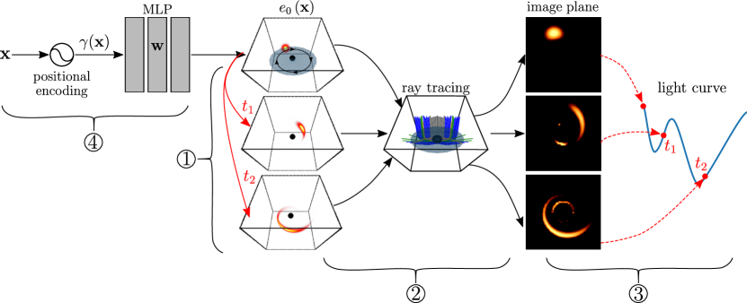
Figure 3: An overview of the orbital tomography framework based on light curve observations. 1. An orbital model propagates an initial (canonical) emission volume ($e_{0}$) in time. 2. Ray tracing: we compute General Relativistic (GR) ray paths according to the black hole parameters and numerically integrate the 3D emissivities to synthesize image plane frames. 3. Each frame is summed to produce a single light curve data point which downstream is compared and adjusted to fit the observations. 4. A neural representation of the underlying 3D volume. Each component is discussed in a corresponding subsection (1.1-1.4)

In this work, we formulate a novel approach for estimating an evolving 3D structure around a black hole from light curve observations. To solve a tomography from a single viewpoint, we rely on both radiative emission and gravitational physics around the black hole. Integrating these physical models with a neural representation of the unknown 3D structure enables solving a highly ill-posed inverse problem which we term “orbital polarimetric tomography”. In the following sections, we describe our methodology and evaluate it on synthetic simulations. Finally, we provide additional analysis of the Sgr A^∗ flare observed by ALMA.

1 Forward model

In this section, we formulate the forward model which takes a canonical 3D emission around a black hole as input and synthetizes light curves as output. Figure 3 provides a high-level overview of the forward model, divided into four key building blocks which we describe in the subsections below.

1.1 Orbit dynamics

The key assumption for orbital tomography is that the 4D (space and time) emission, $e(t,{\bf x})$, is in orbit around the black hole and can be modeled as a simple transformation of a canonical (or initial) 3D emission $e_{0}({\bf x})$:

$$e(t,{\bf x})=e_{0}({\bf T}_{t}{\bf x}),$$ (1)

The transformation ${\bf T}_{t}$ enables propagating an initial 3D structure in time and connects temporal observations, such as light curves, to the canonical 3D structure. This in turn enables formulating an inverse problem of estimating $e_{0}({\bf x})$ from time-variable observations. While the assumption of a coordinate transformation does not hold in general, it is well suited for compact bright structures over short time scales, during which complex dynamics are negligible.

In our work, we consider a Keplerian orbit model with an angular velocity:

$$\Omega(r)=\frac{\sqrt{M}}{r^{3/2}+a\sqrt{M}},$$ (2)

where $r$ is the distance from the black-hole center and $M$ is the black-hole mass. Note that for $a=0$ Eq. (2) coincides with the Newtonian expression for angular velocity. A purely azimuthal orbit is suitable outside the innermost stable circular orbit (ISCO), where radial velocities play a smaller role. Thus, we formulate the coordinate transformation as a shearing operation:

$${\bf T}_{t}={\bf S}_{\phi},$$ (3)

where ${\bf S}_{\phi}$ is a rotation matrix at an angle:

$$\phi\left(t,r\right)=(t-t_{0})\Omega(r).$$ (4)

The angular velocity dependence on $r$ (Eq. 2) causes shearing due to the faster motion of inner radii.

1.2 Image formation

In this section, we describe how $e_{0}$ relates to light curve observations through an image-formation model. Each image pixel collects radiation along a geodesic curve: $\Gamma({\bf\Theta},\alpha,\beta)$ terminating at the image coordinates $(\alpha,\beta)$. The ray path $\Gamma$ is determined by a handful of black hole parameters: ${\bf\Theta}$. Omitting the explicit dependency on image coordinates (for brevity), we model image pixels through the polarized radiative transfer [22, 5, 4] of an optically thin disk:

$${\bf p}(t)=\begin{bmatrix}p_{I}(t)\\ p_{Q}(t)\\ p_{U}(t)\\ p_{V}(t)\end{bmatrix}=\!\!\!\!\!\int\limits_{{\bf x}\in\Gamma({\bf\Theta})}\!\!\!\!\!\!\!g({\bf x})^{2}e(t{+}\tau_{\bf x},{\bf x}){\bf R}({\bf x}){\bf J}({\bf x})d{\bf x}.$$ (5)

The factor $g$ accounts for Doppler boosting. The vector ${\bf J}$ contains the Stokes components of the emitted synchrotron radiation and ${\bf R}$ accounts for the rotation of the linear polarization (LP) components due to the curvature of spacetime (parallel-transport). The integral Eq. (5) is computed along geodesic curves $\Gamma$, which are ray-traced [3] by solving a set of differential equations (see Appendix).

Polarized radiative transfer
Equation (5) describes how pixel values are computed through a geodesic integral over five elements: $g$, $e$, ${\bf R}$ and ${\bf J}$. $e(t{+}\tau_{\bf x},{\bf x})$ is the unknown scalar emissivity that depends on microphysical properties (e.g. local electron density and temperature) and $\tau_{\bf x}$ is the time delay that accounts for photon travel time (often referred to as slow-light). The polarized synchrotron radiation is comprised of this scalar density function multiplied by a Stokes-vector ${\bf J}$ proportional to [9]

$$J_{I} \propto g^{\alpha_{\nu}}\left(|{\bf B}|\sin\phi_{B}\right)^{\alpha_{\nu}+1}$$ (6)

$$J_{Q} \propto q_{f}J_{I}$$ (7)

$$J_{U} =0$$ (8)

In this work, we consider only linear polarization setting $J_{V}=0$. Moreover, the spectral index (reflecting the change in the local emission with frequency) is approximated as $\alpha_{\nu}\simeq 1$ [23]. Note that the local emission frame is defined to align with Stokes-$Q$, therefore, $J_{U}\equiv 0$. The scaling factor $q_{f}\in[0,1]$ is the (volumetric) fraction of linear polarization and $\phi_{B}$ is the angle between the local magnetic field $\bf B$ and photon momentum $\bf k$, given by

$$\sin\phi_{B}({\bf x})=\frac{{\bf k}({\bf x})\times{\bf B}({\bf x})}{\left|{\bf k}({\bf x})\right|\left|{\bf B}({\bf x})\right|}$$ (9)

The two remaining quantities to define are ${\bf R}$ and $g$. The matrix ${\bf R}$ rotates the LP, $(J_{Q},J_{U})$, from the emission frame to the image coordinates through parallel-transport [15] (see Appendix). The scalar field $g({\bf x})$ is a General Relativistic (GR) red-shift factor, which decreases the emission when the material is deep in the gravitational field or moving away from the observer. More generally $g({\bf x})$ depends on the local direction of motion, ${\bf u}$, relative to the photon momentum ${\bf k}$

$$g({\bf x})=\big{\langle}{\bf u}({\bf x}),{\bf k}({\bf x})\!\big{\rangle}$$ (10)

Note that ${\bf u},{\bf k}$ are 4-vectors, more explicitly defined in the Appendix.

1.3 light curves

For a given 3D emission, Eq. (5) enables computing a single pixel value over time. We compute light curves by numerically sampling a large field-of-view (FOV) and summing over image-plane coordinates:

$${\bf I}(t)=\begin{bmatrix}I_{I}(t)\\ I_{Q}(t)\\ I_{U}(t)\\ I_{V}(t)\end{bmatrix}=\sum\limits_{\alpha,\beta}{\bf p}(t,\alpha,\beta)$$ (11)

1.4 Neural representation and implicit regularization

We formulate a tomographic recovery relying on a “neural representation” [21, 20] of the unknown 3D volume: $e_{0}({\bf x})$. Thus, instead of a traditional voxel discretization, the volume is represented by the weights, ${\bf w}$, of a multilayer perceptron (MLP), that are adjusted to fit the observations.

The implicit regularization of the multilayer perceptron (MLP) architecture enables tackling highly ill-posed inverse problems [20, 28]. The MLP takes continuously-valued coordinates ${\bf x}$ as input, and outputs the corresponding scalar emission at that coordinate:

$$e_{0}\left({\bf x}\right)=\operatorname{MLP}_{{\bf w}}(\gamma({\bf x})),$$ (12)

where $\gamma({\bf x})$ is a positional encoding of the input coordinates.

Studies have shown [25] that encoding the coordinates, instead of directly taking them as inputs, can capture continuous fields better (converging in the width limit to a stationary interpolation kernel [16]). Thus, our work relies on a positional encoding that projects each coordinate onto a set of sinusoids with exponentially-increasing frequencies:

$$\gamma({\bf x}){=}\Big{[}\sin({\bf x}),\cos({\bf x}),\ldots,\sin\!\big{(}2^{L-1}{\bf x}\big{)},\cos\!\big{(}2^{L-1}{\bf x}\big{)}\Big{]}^{T}$$ (13)

The positional encoding controls the underlying interpolation kernel used by the MLP, where the parameter $L$ determines the bandwidth of the interpolation kernel [25].

In our work, we use a small MLP with 4 fully-connected layers, where each layer is 128 units wide and uses ReLU activations. We use a maximum positional encoding degree of $L=3$. The low degree of $L$ is suitable for volumetric emission fields which are naturally smooth [20].

2 Optimization: solving the inverse problem

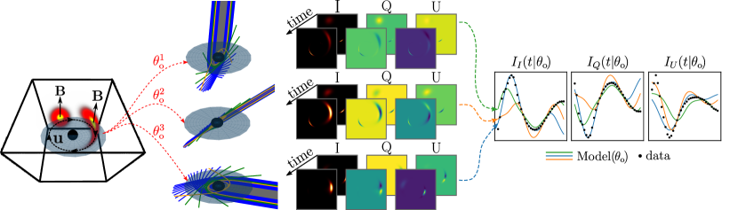
Figure 4: The light curves: $I_{I},I_{Q},I_{U}$, depend on the unknown inclination angle: $\theta_{\rm o}$. This figure illustrates how each inclination angle results in a different image-plane and subsequently light curve model fit. From left to right: 1. An emission bright spot with azimuthal velocity ${\bf u}$ orbits a black hole on the equatorial plane. The vertical magnetic field ${\bf B}$ induces polarized synchrotron radiation. 2. Geodesic curves are computed for every pixel at each inclination angle. 3. Integrating emission along geodesics (Eq. 5) generates a Stokes image plane over time. 4. Summing over image pixels gives the model prediction per inclination angle.

In this section, we formulate an optimization approach that enables jointly estimating the 3D emission and inclination, which are the parameters of the forward model. Figure 4 shows a high-level illustration of the data-fitting procedure introduced in the following section.

2.1 Tomographic reconstruction

To estimate the 3D emission from light curve observations, we formulate a minimization problem. We estimate ${\bf w}$, which parameterizes $e_{0}({\bf x})$, by minimizing a $\chi^{2}$ data fit for each Stokes component, evaluated for a fixed set of black-hole parameters:

$$\mathcal{\chi}^{2}({\bf w}|{\bf\Theta})=\mathcal{\chi}^{2}_{I}({\bf w}|{\bf\Theta})+\mathcal{\chi}^{2}_{Q}({\bf w}|{\bf\Theta})+\mathcal{\chi}^{2}_{U}({\bf w}|{\bf\Theta}).$$ (14)

Here, we restrict the discussion to the total intensity and LP components: $I,Q,U$. Each $\chi^{2}$ is calculated as a sum over discrete temporal data points

$$\mathcal{\chi}^{2}_{s}({\bf w}|{\bf\Theta})=\sum\limits_{i}\left(\frac{{\bf y}_{s}(t_{i})-I_{s}(t_{i},{\bf w}|{\bf\Theta})}{\sigma_{s}}\right)^{2},$$ (15)

where the subscript $s=\left\{I,Q,U,V\right\}$ represents the stokes components, ${\bf y}_{s}$, $I_{s}$ and $\sigma_{s}$ are the polarimetric observations, model, and noise standard deviation respectively. We model the data as homoscedatic ($\sigma_{s}(t_{i})=\sigma_{s}$) within a short and stable observation window (as was the case for the ALMA observation interval analysed [27]).

Equation (14) depends on unknown black hole parameters ${\bf\Theta}$. Nevertheless, the mass of Sgr A^∗ can be constrained through stellar dynamics [1, 10]; $M\simeq 4{\times}10^{6}M_{\odot}$ where $M_{\odot}$ denotes solar masses. Furthermore, in the main paper, we showed how the data fit is insensitive to black hole spin. Thus, the only remaining unknown is the inclination angle. To estimate the inclination we numerically bin $\theta_{\rm o}\in[0,\pi/2]$ and recover the 3D emission by minimizing Eq. (14):

$${\bf w}^{\star}(\theta_{\rm o})=\arg\min_{\bf w}\chi^{2}\left({\bf w}|\theta_{\rm o}\right).$$ (16)

A block diagram of this data-fitting procedure is illustrated in Fig. 4. By interpreting Eq. (16) as a function of $\theta_{\rm o}$ we approximate the marginal log-likelihood as

$$\mathcal{L}(\theta_{\rm o}|{\bf y})\propto\chi^{2}(\theta_{\rm o}|{\bf w}^{\star}).$$ (17)

Equation (17) is a zero-order expansion about the maximum likelihood estimator: ${\bf w}^{\star}$.

2.2 Model selection

While Eq. (17) tells us how well each model (inclination) fits the data, it is susceptible to over-fitting. Thus, in order to mitigate over-fitting, we define the following procedure:

1. During optimization, ray positions are fixed to the center of each image pixel. In our recoveries, we use an evenly sampled $64\times 64$ grid for a FOV of $200~{}\mu{\rm as}$.

2. We compute $\chi^{2}$ for perturbed pixel positions (off-center) within a small pixel area. In our recoveries, we used a pixel area of $3.125\times 3.125~{}\mu{\rm as}^{2}$.

3. We average $\chi^{2}$ of 10 randomly sampled (uniform) ray positions to compute $\chi^{2}$ curves.

4. $\theta_{\rm o}^{\star}$ is estimated as the global minimum of the validation $\chi^{2}$.

Through simulations, we highlight how this procedure is a more robust selection criterion for models that are not overfitting the fixed ray positions (Sec. 4.1).

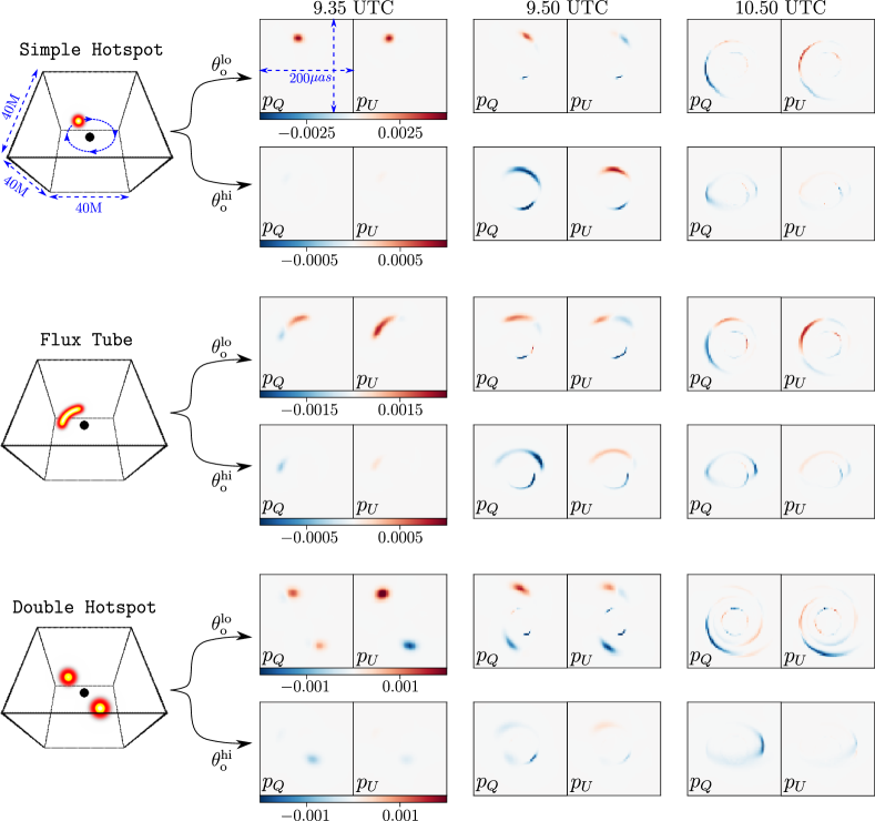
Figure 5: Synthetic simulations of fiducial 3D emission structures: Simple Hotspot, Flux Tube, Double Source. Observations are generated at two inclination angles: $\theta_{\rm o}^{\rm lo}=12^{\circ}$, $\theta_{\rm o}^{\rm hi}=64^{\circ}$. This figure illustrates the gravitationally lensed LP images: $p_{Q},p_{U}$ at three times within a period mimicking the “radio-loops” observed by ALMA: 9.35 – 11 UTC (April 11, 2017). Images are computed at ${\rm FOV}=40M$ ($\sim 200\mu{\rm as}$ for Sgr A^∗) discretized into $64{\times}64$ pixels. To reduce aliasing effects, each pixel is computed as an average of 10 randomly sampled sub-pixel rays. All models share the same dimensions and orbit highlighted in blue for the Simple Hotspot. Note the secondary images formed by gravitational lensing, especially evident in the Simple Hotspot and Flux Tube models (e.g. the bottom half of the image plane at 9.50 UTC)

2.3 Optimization

The neural network was implemented in JAX [2]. Both the synthetic experiments (Sec. 3) and the ALMA recovery (main paper) were optimized using an ADAM optimizer [17] with a polynomial learning rate transitioning from $1{\rm e}^{-4}\rightarrow 1{\rm e}^{-6}$ over $50{\rm K}$ iterations. Run times were ${\sim}1$ hour on two NVIDIA Titan RTX GPUs. Network weights were randomly initialized (Gaussian distributed) with several initial seeds.

3 Synthetic data generation

To quantitatively assess our approach and the ability to recover the 3D structures and constrain an unknown inclination angle we generate synthetic data mimicking ALMA observations. Synthetic simulations allow for careful control of the sources of variability to evaluate the overall impact on the recovery performance. Each dataset consists of a flare on top of a background accretion disk as described in the following sections.

3.1 Emission flares

We generate data consisting of three fiducial distributions of $e_{0}({\bf x})$: Simple Hotspot, Flux Tube, Double Source (Fig. 5). Each volume spans a $40\times 40\times 40~{}[{\rm M}^{3}]$ cube with emission occupying an equatorial disk of $\sim 4-6M$ thickness. For these simulations, we assume a non-spinning black hole with a constant vertical magnetic field ${\bf B}({\bf x})=\hat{\bf z}B_{z}$. We model flares with high fractional polarization resulting in average fluxes matching the real ALMA data [26]

$$\bar{I}_{I} \simeq 0.3-0.4~{}\text{Jy},$$ (18)

$$\bar{P} =\sqrt{I_{Q}^{2}+I_{U}^{2}}\simeq 0.1-0.15~{}\text{Jy}.$$ (19)

Image frames and subsequent light curves are computed by discretizing an FOV of $40M$ (${\sim}200\mu{\rm as}$ for Sgr A^∗) into $64{\times}64$ pixels. Each pixel value is computed by ray-tracing and averaging 10, uniformly randomly sampled, sub-pixel rays. For each 3D structure, observations are generated at two inclination angles: $\theta_{\rm o}^{\rm lo}=12^{\circ}$ and $\theta_{\rm o}^{\rm hi}=64^{\circ}$ resulting in a dataset of six polarimetric light curve observations. Figure 5 illustrates the 3D geometry and a sample of gravitationally lensed linearly polarized frames.

For each fiducial emission, we synthesize $\sim 100$ minutes of observations (9.35 – 11 UTC) to mimic the (time-averaged) ALMA observations used for the reconstruction of the Galactic Center flare. We use a sampling cadence of $\sim 1$ data point per minute with appropriate scan gaps taken from the observational data (see illustration in Fig. 6 bottom panel).

To produce fluxes that are comparable to ALMA observed fluxes, we adjust the magnitude of the 3D emission structure and the volumetric LP fraction (Eq. 8) to satisfy Eqs. (18)–(19). We use a $q_{f}=0.85$ to generate observations at $\theta_{\rm o}^{\rm lo}$ and $q_{f}=0.5$ for $\theta_{\rm o}^{\rm hi}$; A lower $q_{f}$ is used at a high inclination to account for the stronger Doppler boosting (see an analysis of Doppler effects on recovery below).

3.2 Accretion disk

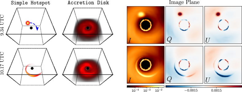
Figure 6: An illustration of the Simple Hotspot and Accretion Disk used for background noise. [left panels] Evolving 3D emission at three different times (rows). [right panels] Corresponding image frames ray-traced for a non-spinning black hole at a low inclination angle ($\theta_{\rm o}^{\rm lo}$). The bright ring is caused by gravitational lensing of the accretion disk with a diameter of $\sim 50~{}\mu{\rm as}$ consistent with the images of Sgr A^∗ [6].

While ALMA observations have low instrumental noise ($\sim 2$ orders of magnitude less than the signal), a significant source of systematic noise is the unaccounted-for variability of the background accretion disk. To assess the impact the background signal has on reconstructions we generate synthetic data of a dynamic accretion disk. We model the accretion disk as a stochastic flow designed to mimic the statistics around Sgr A^∗ [7, 19]. The 2D spiral flow is generated as a Gaussian Random Field (GRF) [18] which is inflated to 3D through convolution with a 1D vertical Gaussian kernel with a full-width half max (FWHM) of $2.35{\rm M}$. Subsequently, the 3D flow is gravitationally lensed (with the same ray-tracing procedure described for the foreground emission flares) to generate a polarized image plane. Figure 6 illustrates the 3D evolution of a randomly sampled Accretion Disk alongside the Simple Hotspot. Furthermore, the integrated image plane(containing both components) is shown at two different evolution times.

4 Tomographic recovery: synthetic data

In this section, we study the recovery performance through experiments designed to highlight different aspects of the tomography approach. In all recoveries, the 3D structure is visualized by sampling the network on a 3D grid at a resolution of $\sim 0.15{\rm M}$. The visualized volumes are in-fact the estimated intrinsic 3D emission (without spacetime curvature).

4.1 Estimating inclination

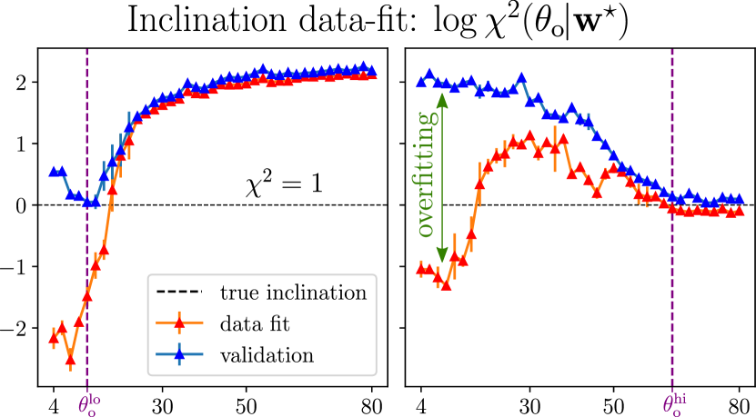
Figure 7: Inclination vs validation $\chi^{2}$ for a Simple Hotspot flare with background accretion noise: $\sigma_{P}=0.01$. The left/right panels show the $\chi^{2}$ for the true low/high inclinations. The right panel highlights how even when the true inclination is $\theta_{\rm o}^{\rm hi}$, low inclination angles are prone to overfitting the data. The validation $\chi^{2}$ (Sec. 2.2) mitigates over-fitting and enables estimating the underlying inclination angle as the global minimum.

In Sec. 2.2 we described an approach for estimating the inclination angle from polarized light curve data. Using the Simple Hotspot model with background accretion noise ($\sigma_{P}$) we show how the conditional $\chi^{2}(\theta_{\rm o}|{\bf w}^{\star})$ enables differentiating $\theta_{\rm o}^{\rm lo}$ from $\theta_{\rm o}^{\rm hi}$ (Fig. 7). The right panel of Fig. 7 highlights the overfitting gap, illustrating how low inclination angles are prone to overfitting. Intuitively, this is because a high inclination provides a stronger physical constraint, requiring the 3D emission to “disappear” behind the black hole for parts of the orbit. Nevertheless, the validation curves (Fig. 7) mitigate over-fitting and enable estimating $\theta_{\rm o}^{\star}$ (as the global minimum) to within $\pm 10^{\circ}$ of the underlying true inclination. Intuitively, this is because recovered overfit structures (${\bf w}^{\star}$) do not generalize as well and are less stable under pixel perturbations.

4.2 Sensitivity to background noise

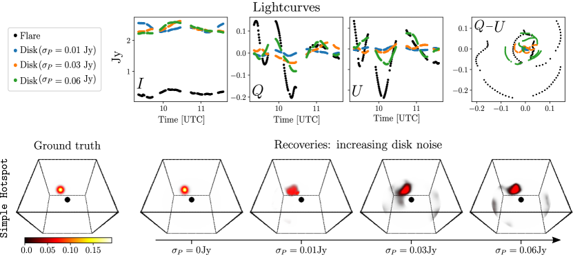
Figure 8: [Top] A comparison between the foreground flare and background accretion disk light curves (noise) for three levels of disk variability $\sigma_{P}=\{0.01,0.03,0.06\}~{}{\rm Jy}$. [Bottom] 3D reconstructions for the three levels of disk variability. These volumes represent the true/estimated initial emission at 9.35 UTC. In all cases, our approach is able to estimate the inclination angle within $\pm 4^{\circ}$ (see Fig. A in the Appendix). Under each estimate, $\theta_{\rm o}^{\star}$ the recovered 3D emission captures the key features of the underlying true flare structure.

In reality, observed variability is due to both the flare and accretion flow, however, it is difficult to determine the relative contributions of each source. In this section, we explore the impact of different accretion flow variability. This un-modeled dynamic component impacts recovery results as our model fully attributes dynamics to orbital motion. By sampling random accretion flows and varying the degree of polarization ($q_{f}=\{0.25,0.5,0.75\}~{}{\rm Jy}$) we generate noise light curves with $\sigma_{P}=\{0.01,0.03,0.06\}~{}{\rm Jy}$.

Similar to the pre-processing of ALMA data [26], we subtract the time-averaged LP component (the static component of the background emission). A comparison between the simulated Simple Hotspot flare and accretion disk light curves, for different levels of variability, is shown in Figure 8 (top panels). In these simulations, the underlying true inclination is $\theta_{\rm o}^{\rm lo}$. For each level of noise, $\sigma_{P}$, we are able to estimate $\theta_{\rm o}^{\star}$ to within $\pm 4^{\circ}$ of the true value.

using the validation-$\chi^{2}$ minimum, our approach is able to recover the inclination angle to within $\pm 4^{\circ}$ of the true value ($\chi^{2}$ curves in Appendix Fig. A). Subsequently, using the estimate $\theta_{\rm o}^{\star}$, we recover the unknown 3D emission. Figure 8 shows a comparison between the recovered 3D emission and the ground truth. As the unaccounted disk variability increases, more emission is attributed sporadically within the volume. Nevertheless, the compact hotspot remains the brightest feature in the recovered 3D volume centered around the true azimuthal position.

4.3 Recovering different 3D morphology

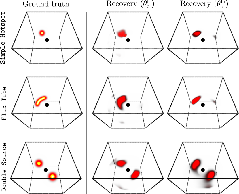
Figure 9: 3D recoveries compared to the ground truth for each fiducial distribution observed with two inclination angles: $\theta_{\rm o}^{\rm lo}/\theta_{\rm o}^{\rm hi}$. The recovered structure is given under an inclination $\theta_{\rm o}^{\star}$ that minimizes the validation-$\chi^{2}$ (Fig. 7 shows the data-fit/validation for the Simple Hotspot case).

In these simulations, we highlight the tomographic ability to recover different underlying emission structures and distinguish between different 3D flare morphologies.

For each of the fiducial datasets (Fig. 5) we add accretion disk noise with $\sigma_{P}=0.01~{}\text{Jy}$ and estimate the inclination angle, $\theta_{\rm o}^{\star}$ as the minimum in the validation-$\chi^{2}$ (curves are given in Fig. A in the Appendix). In all cases, our approach is able to accurately recover $\theta_{\rm o}^{\rm lo}$ and recover $\theta_{\rm o}^{\rm hi}$ to within $\pm 10^{\circ}$ of the true value. Figure 9 highlights how our approach is able to simultaneously estimate an unknown inclination and 3D structure from unresolved light curve observations. In each case, the recovered 3D captures the unique morphology of the underlying ground truth structure and is smoothed out by the tomographic reconstruction process.

It is instructive to visualize noise present in the 3D reconstructions. To illustrate noisy features we recover the 3D volume of a stochastic disk, without an orbiting bright flare, from light curve observations. In these recoveries the dynamic signal does not conform to the model assumptions made by the orbital tomography algorithm as brightness does not merely orbit and shear but also appears and disappears. Figure 10 demonstrates the 3D reconstructions with different random seeds (initial conditions for the neural network / 3D volume). Under certain initializations compact emission may appear, however, in contrast to the reconstructions of flares, these components are not stable. The consistent artifacts at the boundary, also present in the real data reconstructions (Figs. 1, 15), suggest these are likely an artifact of the reconstruction algorithm.

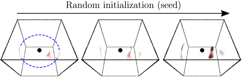
Figure 10: 3D reconstruction of a stochastic accretion disk (Fig. 6) without an orbiting bright flare. In these recoveries the observed dynamic signal does not follow the assumptions of orbital tomography. Different initializations (seeds) lead to different local minima. Visualizing the converged solutions gives a sense of the artifacts that would appear in a real data reconstruction (the color bar matches Fig. 8) The domain boundary is highlighted in blue in the leftmost recovery.

4.4 Recovery blind spot

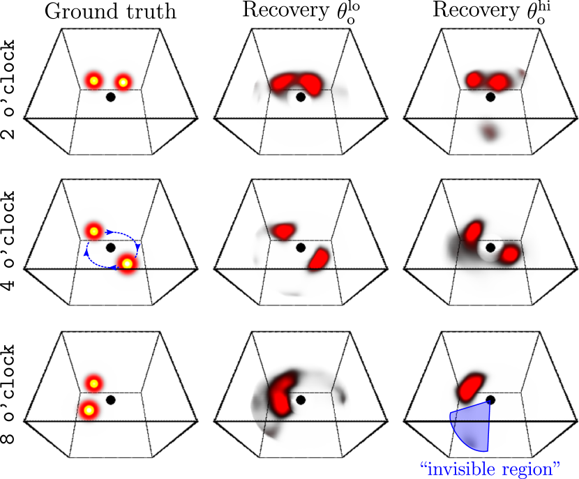
Figure 11: 3D recoveries of two sources in a clockwise orbit. The initial position of one source is fixed 11 o’clock and the other at 2/4/8 o’clock (different rows). Each column represents recoveries with observations at a different inclination angle $\theta_{\rm o}^{\rm lo}/\theta_{\rm o}^{\rm hi}$. Doppler boosting acts to dim sources moving away from the observer resulting in a “blind spot” (highlighted in blue) at high inclination angles. Nevertheless, for the 2/4 o’clock orbital configurations our approach is able to recover the distinct structure of two emission sources.

Close to the event horizon, gas is orbiting at relativistic velocities resulting in a substantial Doppler boosting effect, Doppler boosting effects are particularly strong at high inclination angles where emission moving away appears very faint compared to emission moving towards the observer. This is clearly illustrated in Fig. 5 where one of the bright spots in the Double Source images is extremely faint due to the clockwise rotational motion. For this reason, we anticipate that reconstruction errors will not be distributed equally across the orbital plane.

To test this hypothesis we simulate observations with two sources, one at a fixed 11 o’clock azimuthal position and the other at variable 2/4/8 o’clock positions (Fig. 11). The recoveries shown in Fig. 11 reveal an “invisible region” at high inclination angles where sources are dim due to Doppler boosting. Due to recovery blurring, bright features that are close together merge to form a single region (see 2/4/8 o’clock positions in Fig. 11). Nevertheless, these regions contain two distinct brightness peaks attributed to the two hotspots. The Doppler boosting effects are weaker at low inclination angles which are favored by the real data fit.

5 ALMA observations: extended analysis

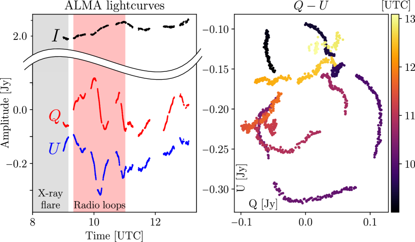
Figure 12: Linear polarization of ALMA at 229 GHz. The light curves were observed on 2017 April 11 (MJD 57854) as part of the EHT Sgr A^∗ campaign. The red-shaded region corresponds to a time of period $\sim 100$ minutes in which polarimetric (Q-U) loops are apparent directly after an X-ray flare was observed (gray-shaded region). The rotation of the polarization angle at a period similar to a Keplerian orbital period suggests the signal is coming from a bright compact structure in orbit around Sgr A^∗ [26].

In the main paper, we showed recovery results and analysis of a galactic flare through ALMA polarimetric observations on April 11, 2017 at 9:20 UT. In this section, we present an extended analysis of the data and results. Figure 12 shows the radio observations that took place directly after an X-ray flare. The LP curves used for data-fitting were time-averaged over ${\sim}1$ minute intervals resulting in ${\sim}100$ data points for each Stokes component (Fig. 2 in the main text). Following [26] we chose 9:20 UT as the initial time of the analysis of the flare. Figure 13 shows the validation-$\chi^{2}$ for different initial times around 9:20 UT, providing further motivation for the selection of this initial time. For pre-processing we subtract a constant LP component with magnitude and angle of $P_{\rm disk}=0.16~{}\text{Jy}$, $\xi_{\rm disk}=-37^{\circ}$ respectively to account for the background accretion disk; We de-rotate the electric vector polarization angle (EVPA) by $32.2^{\circ}$ to account for the estimated Faraday rotation; and we time average the data over $\sim 35s$ intervals.

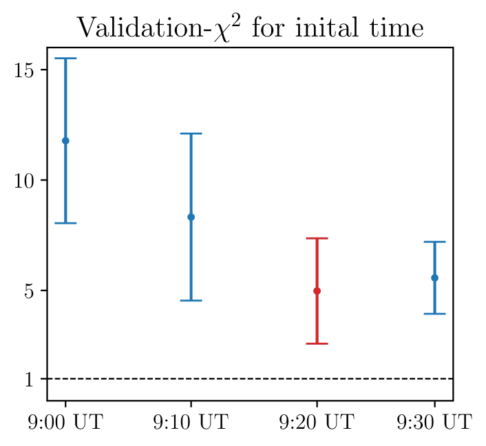
Figure 13: Validation-$\chi^{2}$ for different initial times around the fiducial time of 9:20 UT, which has the best data-fit (lowest validation-$\chi^{2}$) highlighted in red.

5.1 Systematics: magnetic field and velocity

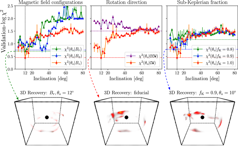
Figure 14: [Top] Validation $\chi^{2}$ as a function of inclination angle for different model choices: magnetic field configuration, rotation direction, and sub-Keplerian fraction. [Bottom] 3D reconstructions under various model assumptions. The red curve in all panels represents the selected fiducial model parameters (3D volume at $\theta_{\rm o}=12^{\circ}$ shown in the center panel) with a vertical magnetic field, $B_{z}$, clockwise rotation (CW), and Keplerian orbit ($f_{\rm K}=1.0$). The global minimum for each curve is highlighted by a horizontal dashed line in the respective color. [Left] Three different magnetic field configurations: vertical, radial, and toroidal (subscripts: $z,r,\phi$ respectively). The recovered 3D under a radial magnetic field appears spread out rather than a compact hot-spot like structure. That being said, consistent with the analysis of [12, 26], vertical magnetic fields, which result in a hotspot-like structure, are favorable according to this metric with lower validation-$\chi^{2}$ around $\theta_{\rm o}=12^{\circ}$. [Center] A comparison of clockwise (CW) and counter-clockwise (CCW) angular velocity models. Consistent with the analysis of [26], a CW rotation is preferred across all inclination angles. [Right] A Keplerian orbit has the lowest validation-$\chi^{2}$ fit across three different fractions of sub-Keplerian orbit: $f_{\rm K}=1.0,0.9,0.8$. The recovery under $f_{\rm K}=0.9$ (bottom right) is broadly consistent with the fiducial (Keplerian) model.

The analysis in the paper assumes a fixed, homogeneous, vertical magnetic field and a clockwise rotation at a Keplerian orbit. Both of these assumptions are a source of systematic error in the reconstructions. In this section, we analyze these model choices, which are motivated by prior studies [12, 26], using the validation-$\chi^{2}$ (described in Sec. 2.2). It is important to note that we do not aim to exhaustively test all possible magnetic field and orbital velocity models, but instead highlight the sensitivity of our reconstruction to these model choices.

The left panel of Fig. 14 compares the validation curves for three magnetic field configurations: vertical, radial, and toroidal, respectively denoted by subscripts: $z,r,\phi$. For each curve, the global minimum is highlighted by a dashed line at the respective color. The choice of a vertical magnetic field for the fiducial recovery is motivated by the notion that vertical magnetic fields could be powering Sgr A^∗ flares, apparent in GRMHD simulation producing magnetic eruption events [24]. Moreover, from an observational standpoint, vertical magnetic fields are preferred by both the near infrared analysis of GRAVITY [12, 13, 14] and mm ALMA analysis of [26]. Nevertheless, the true spatial structure and dynamic properties of the magnetic fields around Sgr A^∗ are largely unknown. By comparing validation-$\chi^{2}$ we test the sensitivity of the recovery to the magnetic field orientation. For a radial magnetic field, the best fit recovery is not a compact bright emission region (Fig. 14 bottom left). Rather, it is a fainter diffuse structure. Even so, according to the data-fit, and consistent with prior studies, vertical magnetic fields are preferred with a lower validation-$\chi^{2}$ value.

The center and rightmost panels in Fig. 14 highlight how clockwise rotation (CW) and a Keplerian orbit are favorable to counter-clockwise rotation (CCW) or sub-Keplerian orbits, consistent with the analyses of GRAVITY [14], and [26]. To test the fit of orbit direction and sub-Keplerian fraction we set the angular velocity profile to $\Omega=\pm f_{\rm K}\Omega_{\rm K}$ where the $\pm$ sign dictates the direction (CW/CCW) and $f_{\rm K}$ the magnitude ($f_{\rm K}=1$ results in a Keplerian orbit). The 3D recovery under the assumption of $f_{\rm K}=0.9$ is shown in the bottom-right panel of Fig. 14 highlighting a broadly consistent recovery with the fiducial model assumptions at this perturbation. However, this consistency eventually breaks down at strong deviations from the Keplarian velocity assumption (also resulting in lower validation-$\chi^{2}$ values).

5.2 3D recovery variability

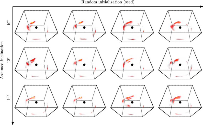
Figure 15: A visualization of 3D recoveries across different inclinations and initial conditions (Fig. 15). While the details of each recovered structure depend on both axes, some key features remain consistent. While the exact angular extent of the structures is not stable, the azimuthal and radial position appears stable and consistent with the average structure highlighted in Fig. 1 in the paper. Moreover, the separation into distinct emission regions of an elongated feature trailed by a smaller compact bright spot appears consistent across the different recoveries.

While our approach is successful in recovering 3D structures in simulations the ill-posed inverse problem we solve does not have a unique solution. The recovered 3D structure depends, among other factors, on the assumed inclination angle. Furthermore, solving a non-convex optimization with stochastic gradient descent methods leads to a local (and not global) minimum. Thus, the recovered 3D structure also depends on the random initialization of the network weights. In the paper, we showed the average 3D structure across different initializations at the estimated inclination $\theta_{\rm o}^{\star}=12^{\circ}$. To get a sense of the robustness of the 3D structure we recover the emission across different inclinations and initial conditions (Fig. 15). While this is not an exploration of the posterior distribution, the different recoveries give a sense of the solution’s stability. Qualitatively, the details of each recovered structure exhibit dependence on both the inclination angle and initialization. Nevertheless, some key features are consistent across these two axes. While the exact angular extent of the structures is not stable, the azimuthal and radial position appears stable and consistent with the average structure highlighted in Fig. 1 in the paper. Moreover, the separation of the emission into two distinct structures appears consistent across the different recoveries (and average structure).

Appendix A Inclination Estimation

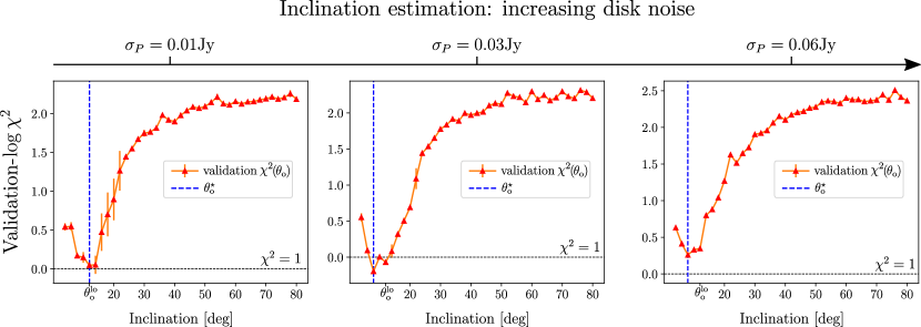
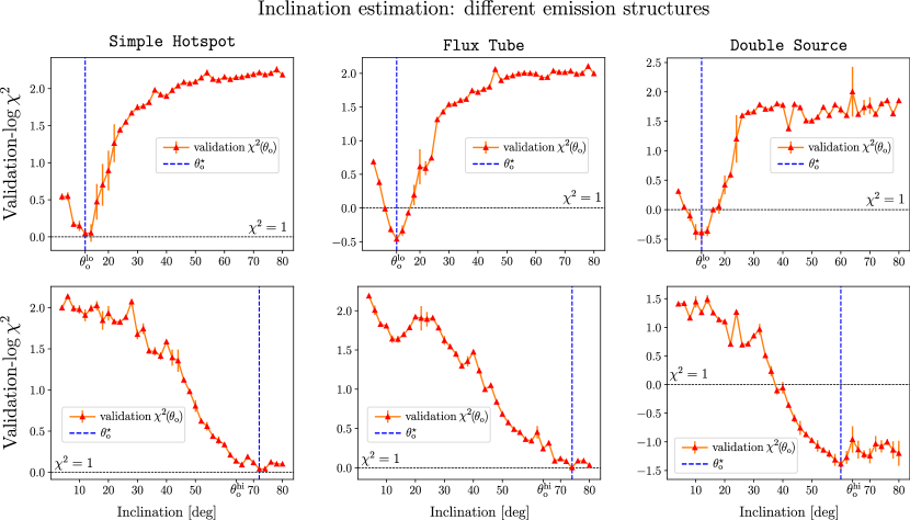
Figure 16: These validation-$\chi^{2}$ curves correspond to the estimated Simple Hotspot volumes with increasing disk variability $\sigma_{P}$ shown in Fig. A. The estimated inclination $\theta_{\rm o}^{\star}$ (blue), estimated as the global minimum, is within $\pm 4^{\circ}$ of the underlying true inclination $\theta_{\rm o}^{\rm lo}$.

Figure 17: These validation-$\chi^{2}$ curves correspond to the estimated volumes of 3D fiducial models with $\sigma_{P}=0.01~{}\text{Jy}$ shown in Fig. 9. The top/bottom rows correspond to a true inclination of $\theta_{\rm o}^{\rm lo}/\theta_{\rm o}^{\rm hi}$ and the estimated inclination $\theta_{\rm o}^{\star}$ (global minimum) is highlighted in blue. For a true inclination $\theta_{\rm o}^{\rm lo}$ the minimum coincides with the true inclination for all three emission structures. For $\theta_{\rm o}^{\rm hi}$ the minimum is within $\pm 10^{\circ}$ of the underlying true inclination.

Appendix B Geodesic Ray Tracing

This section describes the General Relativistic (GR) equations used to compute geodesic paths and polarized radiative transfer described in the forward model (Sec. 1).

B.1 Kerr metric

We work in the Kerr black hole spacetime in units where $G=c=1$. A Kerr black hole has mass $M$ and spin $a$. We use Boyer-Lindquist coordinates, where points in the spacetime are indicated by a four-vector $x^{\mu}=(t,r,\theta,\phi)$.

The structure of spacetime is encoded in the metric $g_{\mu\nu}$, which is a $4\times 4$ symmetric matrix. In Boyer-Lindquist coordinates, the nonzero components of the metric are

$$g_{tt} =-(1-2Mr/\Sigma)$$ (20)

$$g_{rr} =\Sigma/\Delta$$ (21)

$$g_{\theta\theta} =\Sigma$$ (22)

$$g_{\phi\phi} =\Pi\sin^{2}\theta/\Sigma$$ (23)

$$g_{t\phi} =g_{\phi t}=-2Mar\sin^{2}\theta/\Sigma.$$ (24)

where the following are commonly used abbreviations.

$$\Delta =r^{2}+a^{2}-2Mr$$ (25)

$$\Sigma =r^{2}+a^{2}\cos^{2}\theta$$ (26)

$$\Pi =(r^{2}+a^{2})^{2}-a^{2}\Delta\sin^{2}\theta$$ (27)

$$\omega =2aMr/\Pi.$$ (28)

The nonzero components of the inverse metric $g^{\mu\nu}$ are

$$g^{tt} =-\Pi/\Delta\Sigma$$ (29)

$$g^{rr} =\Delta/\Sigma$$ (30)

$$g^{\theta\theta} =1/\Sigma$$ (31)

$$g^{\phi\phi} =(\Delta-a^{2}\sin^{2}\theta)/(\Delta\Sigma\sin^{2}\theta)$$ (32)

$$g^{t\phi} =g^{\phi t}=-2Mar/\Delta\Sigma.$$ (33)

B.2 Ray tracing

We define the image plane of the observer at time $t=0$, at radius $r_{o}\rightarrow\infty$, and at an inclination angle $\theta_{o}$ to the angular momentum axis of the black hole (BH). We use Cartesian coordinates $(\alpha,\beta)$ on the image plane, measured in units of $M$. The origin $\alpha=\beta=0$ is the line of sight to the black hole at $r=0$, and the $+\beta$ image plane axis is parallel with the BH spin direction (i.e. with the $-\theta$ direction).

We solve for the trajectories of photons backward from a specific position $(\alpha,\beta)$ on the image plane using a set of differential equations which in Einstein notation can be written as:

$$\frac{dx^{\mu}}{d\sigma}=k^{\mu}.$$ (34)

Here $\sigma$ is the path parameter (“affine time”) and

$$x^{\mu}(\sigma)=\left(t(\sigma),r(\sigma),\theta(\sigma),\phi(\sigma)\right),$$ (35)

is a parameterized trajectory in spherical (Boyer-Lindquist) coordinates.

Each photon trajectory is defined by three constants of motion: $(E,\lambda,\eta)$. $E$ is photon energy at infinity (i.e., observed frequency). The parameters $\lambda$ (angular momentum) and $\eta$ (Carter constant) are fully determined by the photon’s coordinates on the observer screen:

$$\lambda =-\alpha\sin\theta_{o}$$ (36)

$$\eta =(\alpha^{2}-a^{2})\cos^{2}\theta_{o}+\beta^{2}.$$ (37)

From these constants, at each point along the trajectory, the photon’s covariant momentum (lower index) $k_{\mu}$ is given by [11]:

$$k_{t} =-E$$ (38)

$$k_{r} =\pm E\sqrt{\mathcal{R}(r)}/\Delta$$ (39)

$$k_{\theta} =\pm E\sqrt{\Theta(\theta)}$$ (40)

$$k_{\phi} =E\lambda,$$ (41)

where $\mathcal{R}$ and $\Theta$ are radial and polar potentials:

$$\mathcal{R}(r) =(r^{2}+a^{2}-a\lambda)^{2}-\Delta\left[\eta+(\lambda-a)^{2}\right]$$ (42)

$$\Theta(\theta) =\eta+a^{2}\cos^{2}\theta-\lambda^{2}/\tan^{2}\theta.$$ (43)

The choice of $\pm$ sign in Eq (38–41) depends on the direction of motion (signs reverse at angular and radial turning points when $k^{\theta}=0$ or $k^{r}=0$, respectively.).

Equation (34) is described in terms of the contravariant (upper index) momentum vector $k^{\mu}$, which is obtained by multiplying the covariant momentum (Eqs. 38–41) by the inverse metric

$$k^{\mu}=g^{\mu\nu}k_{\nu}.$$ (44)

To compute geodesic paths $x^{\mu}(\sigma)$, we solve Eq. (34) using the explicit parametric form described by [11] and implemented in [3].

B.3 Fluid Velocity and Redshift

Outside the ISCO, the four-velocity $u^{\mu}$ of prograde circular orbits in the equatorial plane is $u^{\mu}(r)$, where:

$$u^{t} =u^{t}$$ (45)

$$u^{r} =0$$ (46)

$$u^{\theta} =0$$ (47)

$$u^{\phi} =u^{t}\Omega,$$ (48)

Since the four-velocity must be normalized so that $u^{\mu}u_{\mu}=g_{\mu\nu}u^{\mu}u^{\nu}=-1$,

$$u^{t} =\frac{1}{\sqrt{-g_{tt}-2\Omega g_{t\phi}-\Omega^{2}g_{\phi\phi}}}.$$ (49)

The redshift factor $g$ describes the change in frequency of a photon between the observer’s frame at infinity and the frame where it is emitted.

$$g^{-1}=\frac{\nu_{\mathrm{emis}}}{\nu_{\rm obs}}=\frac{-k_{\mu}u^{\mu}}{E}.$$ (50)

B.4 Parallel transport

Ray-tracing polarization on curved spacetime requires parallel transporting the emitted polarization to the observer screen. In Eq. (5) we defined this operation as a rotation matrix: R. This matrix multiplies the emission-frame Stokes vector $\bf J$ to rotate the linearly-polarized components:

$${\bf R}{\bf J}=\begin{bmatrix}1&0&0&0\\ 0&\cos 2\chi&-\sin 2\chi&0\\ 0&\sin 2\chi&\cos 2\chi&0\\ 0&0&0&1\end{bmatrix}\begin{bmatrix}J_{I}\\ J_{Q}\\ 0\\ J_{V}\end{bmatrix}.$$ (51)

The angle $\chi$ at pixel coordinates $(\alpha,\beta)$ is given by [15]:

$$e^{2i\chi}=\frac{(\beta+i\mu)(\kappa_{1}-i\kappa_{2})}{(\beta-i\mu)(\kappa_{1}+i\kappa_{2})},$$ (52)

where $\kappa=\kappa_{1}+i\kappa_{2}$ is the complex Penrose-Walker constant, a quantity that is computed in the emission frame and then conserved in parallel transport, and $\mu=-(\alpha+a\sin\theta_{o})$.

To compute $\kappa$ in the emitter frame we first convert the coordinate-frame 4-vectors $k^{\mu}$ and $b^{\mu}$ for the magnetic field to local 3-vectors $\bf{k}$ and $\bf{B}$ using the tetrad matrices $e^{\mu}_{a}$ (which depend on the emission position and fluid velocity) as described in [5] (Equations 36-42). We then compute the local emitted polarization vector $\bf{f}$ from

$$\mathbf{f}=\frac{\mathbf{k}\times\mathbf{B}}{|\mathbf{k}|}.$$ (53)

We then convert $\bf{f}$ to a coordinate frame four-vector $f^{\mu}$ using the transpose tetrad matrix. The constant $\kappa$ is then [5, 9]

$$\kappa =\kappa_{1}+i\kappa_{2}=(r-ia\cos\theta)(A-iB)$$ (54)

$$A =(k^{t}f^{r}-k^{r}f^{t})+a\sin^{2}\theta(k^{r}f^{\phi}-k^{\phi}f^{r})$$ (55)

$$B =\left[(r^{2}+a^{2})(k^{\phi}f^{\theta}-k^{\theta}f^{\phi})-a(k^{t}f^{\theta}-k^{\theta}f^{t})\right]\sin\theta.$$ (56)

References

- [1] A. E. Broderick and A. Loeb. Imaging bright-spots in the accretion flow near the black hole horizon of Sgr A*. Monthly Notices of the Royal Astronomical Society, 363(2):353–362, October 2005.
- [2] J. Dexter, A. Tchekhovskoy, A. Jiménez-Rosales, S. M. Ressler, M. Bauböck, Y. Dallilar, P. T. de Zeeuw, F. Eisenhauer, S. von Fellenberg, F. Gao, R. Genzel, S. Gillessen, M. Habibi, T. Ott, J. Stadler, O. Straub, and F. Widmann. Sgr A* near-infrared flares from reconnection events in a magnetically arrested disc. Monthly Notices of the Royal Astronomical Society, 497(4):4999–5007, October 2020.
- [3] Event Horizon Telescope Collaboration. First Sagittarius A* Event Horizon Telescope Results. I. The Shadow of the Supermassive Black Hole in the Center of the Milky Way. The Astrophysical Journal Letters, 930(2):L12, May 2022.
- [4] Event Horizon Telescope Collaboration. First Sagittarius A* Event Horizon Telescope Results. II. EHT and Multiwavelength Observations, Data Processing, and Calibration. The Astrophysical Journal Letters, 930(2):L13, May 2022.
- [5] Event Horizon Telescope Collaboration. First Sagittarius A* Event Horizon Telescope Results. III. Imaging of the Galactic Center Supermassive Black Hole. The Astrophysical Journal Letters, 930(2):L14, May 2022.
- [6] Event Horizon Telescope Collaboration. First Sagittarius A* Event Horizon Telescope Results. V. Testing Astrophysical Models of the Galactic Center Black Hole. The Astrophysical Journal Letters, 930(2):L16, May 2022.
- [7] Event Horizon Telescope Collaboration. First Sagittarius A* Event Horizon Telescope Results. VI. Testing the Black Hole Metric. The Astrophysical Journal Letters, 930(2):L17, May 2022.
- [8] G. G. Fazio, J. L. Hora, G. Witzel, S. P. Willner, M. L. N. Ashby, F. Baganoff, E. Becklin, S. Carey, D. Haggard, C. Gammie, et al. Multiwavelength light curves of two remarkable sagittarius a* flares. The Astrophysical Journal, 864(1):58, 2018.
- [9] Z. Gelles, E. Himwich, M. D. Johnson, and D. C. M. Palumbo. Polarized image of equatorial emission in the kerr geometry. Physical Review D, 104(4):044060, 2021.
- [10] R. Genzel, R. Schödel, T. Ott, A. Eckart, T. Alexander, F. Lacombe, D. Rouan, and B. Aschenbach. Near-infrared flares from accreting gas around the supermassive black hole at the galactic centre. Nature, 2003.
- [11] A. M. Ghez, S. Salim, N. N. Weinberg, J. R. Lu, T. Do, J. K. Dunn, K. Matthews, M. R. Morris, S. Yelda, E. E. Becklin, et al. Measuring distance and properties of the milky way’s central supermassive black hole with stellar orbits. The Astrophysical Journal, 689(2):1044, 2008.
- [12] GRAVITY Collaboration. Detection of orbital motions near the last stable circular orbit of the massive black hole SgrA*. Astronomy & Astrophysics, 618:L10, October 2018.
- [13] GRAVITY Collaboration. Modeling the orbital motion of Sgr A*’s near-infrared flares. Astronomy & Astrophysics, 635:A143, March 2020.
- [14] Gravity Collaboration. Polarimetry and astrometry of NIR flares as event horizon scale, dynamical probes for the mass of Sgr A*. Astronomy & Astrophysics, 677:L10, September 2023.
- [15] D. Haggard, M. Nynka, B. Mon, N. de la Cruz Hernandez, M. Nowak, C. Heinke, J. Neilsen, J. Dexter, P. Chris Fragile, F. Baganoff, G. C. Bower, L. R. Corrales, F. Coti Zelati, N. Degenaar, S. Markoff, M. R. Morris, G. Ponti, N. Rea, J. Wilms, and F. Yusef-Zadeh. Chandra Spectral and Timing Analysis of Sgr A*’s Brightest X-Ray Flares. The Astrophysical Journal, 886(2):96, December 2019.
- [16] A. Levis, P. P. Srinivasan, A. A. Chael, R. Ng, and K. L. Bouman. Gravitationally lensed black hole emission tomography. In Proceedings of the IEEE/CVF Conference on Computer Vision and Pattern Recognition, pages 19841–19850, 2022.
- [17] D. P. Marrone, F. K. Baganoff, M. R. Morris, J. M. Moran, A. M. Ghez, S. D. Hornstein, C. D. Dowell, D. J. Muñoz, M. W. Bautz, G. R. Ricker, W. N. Brandt, G. P. Garmire, J. R. Lu, K. Matthews, J. H. Zhao, R. Rao, and G. C. Bower. An X-Ray, Infrared, and Submillimeter Flare of Sagittarius A*. The Astrophysical Journal, 682(1):373–383, July 2008.
- [18] B. Mildenhall, P. P. Srinivasan, M. Tancik, J. T. Barron, R. Ramamoorthi, and R. Ng. NeRF: Representing scenes as neural radiance fields for view synthesis. ECCV, 2020.
- [19] J Neilsen, M. A. Nowak, C Gammie, J Dexter, S Markoff, D Haggard, S Nayakshin, Q. D. Wang, N Grosso, D Porquet, et al. A chandra/hetgs census of x-ray variability from sgr a* during 2012. The Astrophysical Journal, 774(1):42, 2013.
- [20] B. Ripperda, M. Liska, K. Chatterjee, G. Musoke, A. A. Philippov, S. B. Markoff, A. Tchekhovskoy, and Z. Younsi. Black hole flares: ejection of accreted magnetic flux through 3d plasmoid-mediated reconnection. The Astrophysical Journal Letters, 924(2):L32, 2022.
- [21] M.!Tancik, P. P. Srinivasan, B. Mildenhall, S. F. Keil, N. Raghavan, U. Singhal, R. Ramamoorthi, J. T. Barron, and R. Ng. Fourier features let networks learn high frequency functions in low dimensional domains. NeurIPS, 2020.
- [22] P. Tiede, H. Y. Pu, A. E. Broderick, R. Gold, M. Karami, and J. A. Preciado-López. Spacetime Tomography Using the Event Horizon Telescope. The Astrophysical Journal, 892(2):132, April 2020.
- [23] J. Vos, M. A. Mościbrodzka, and M. Wielgus. Polarimetric signatures of hot spots in black hole accretion flows. Astronomy & Astrophysics, 668:A185, December 2022.
- [24] M. Wielgus, M. Moscibrodzka, J. Vos, Z. Gelles, I. Martí-Vidal, J. Farah, N. Marchili, C. Goddi, and H. Messias. Orbital motion near Sagittarius A∗ . Constraints from polarimetric ALMA observations. Astronomy & Astrophysics, 665:L6, September 2022.
- [25] M. Wielgus, N. Marchili, I. Martí-Vidal, G. K. Keating, V. Ramakrishnan, P. Tiede, E. Fomalont, S. Issaoun, J. Neilsen, M. A. Nowak, et al. Millimeter Light Curves of Sagittarius A* Observed during the 2017 Event Horizon Telescope Campaign. The Astrophysical Journal Letters, 930(2):L19, May 2022.
- [26] G. Witzel, G. Martinez, S. P. Willner, E. E. Becklin, H. Boyce, T. Do, A. Eckart, G. G. Fazio, A. Ghez, M. A. Gurwell, D. Haggard, R. Herrero-Illana, J. L. Hora, Z. Li, J. Liu, N. Marchili, M. R. Morris, H. A. Smith, M. Subroweit, and J. A. Zensus. Rapid Variability of Sgr A* across the Electromagnetic Spectrum. The Astrophysical Journal, 917(2):73, August 2021.

References

- [1] R Abuter, N Aimar, A Amorim, J Ball, M Bauböck, JP Berger, H Bonnet, G Bourdarot, W Brandner, V Cardoso, et al. Mass distribution in the galactic center based on interferometric astrometry of multiple stellar orbits. Astronomy & Astrophysics, 657:L12, 2022.
- [2] J. Bradbury, R. Frostig, P. Hawkins, M. J. Johnson, C. Leary, D. Maclaurin, G. Necula, A. Paszke, J. VanderPlas, S. Wanderman-Milne, and Q. Zhang. JAX: composable transformations of Python+NumPy programs, 2018.
- [3] A Chael. kgeo (version 1.0.0). https://github.com/achael/kgeo, 2023. Online; accessed 01-June-2023.
- [4] CK. Chan, D. Psaltis, and F. Özel. GRay: A Massively Parallel GPU-based Code for Ray Tracing in Relativistic Spacetimes. The Astrophysical Journal, 777(1):13, November 2013.
- [5] J. Dexter. A public code for general relativistic, polarised radiative transfer around spinning black holes. Monthly Notices of the Royal Astronomical Society, 462(1):115–136, October 2016.
- [6] Event Horizon Telescope Collaboration. First Sagittarius A* Event Horizon Telescope Results. I. The Shadow of the Supermassive Black Hole in the Center of the Milky Way. The Astrophysical Journal Letters, 930(2):L12, May 2022.
- [7] Event Horizon Telescope Collaboration. First Sagittarius A* Event Horizon Telescope Results. III. Imaging of the Galactic Center Supermassive Black Hole. The Astrophysical Journal Letters, 930(2):L14, May 2022.
- [8] Event Horizon Telescope Collaboration. First Sagittarius A* Event Horizon Telescope Results. V. Testing Astrophysical Models of the Galactic Center Black Hole. The Astrophysical Journal Letters, 930(2):L16, May 2022.
- [9] Zachary Gelles, Elizabeth Himwich, Michael D Johnson, and Daniel CM Palumbo. Polarized image of equatorial emission in the kerr geometry. Physical Review D, 104(4):044060, 2021.
- [10] A. M. Ghez, S. Salim, N. N. Weinberg, J. R. Lu, T. Do, J. K. Dunn, K. Matthews, M. R. Morris, S. Yelda, E. E. Becklin, et al. Measuring distance and properties of the milky way’s central supermassive black hole with stellar orbits. The Astrophysical Journal, 689(2):1044, 2008.
- [11] S. E. Gralla and A. Lupsasca. Null geodesics of the kerr exterior. Physical Review D, 101(4):044032, 2020.
- [12] GRAVITY Collaboration. Detection of orbital motions near the last stable circular orbit of the massive black hole SgrA*. Astronomy & Astrophysics, 618:L10, October 2018.
- [13] GRAVITY Collaboration. Modeling the orbital motion of Sgr A*’s near-infrared flares. Astronomy & Astrophysics, 635:A143, March 2020.
- [14] Gravity Collaboration. Polarimetry and astrometry of NIR flares as event horizon scale, dynamical probes for the mass of Sgr A*. Astronomy & Astrophysics, 677:L10, September 2023.
- [15] E. Himwich, M. D. Johnson, A. Lupsasca, and A. Strominger. Universal polarimetric signatures of the black hole photon ring. Physical Review D, 101(8):084020, 2020.
- [16] A. Jacot, F. Gabriel, and C. Hongler. Neural tangent kernel: Convergence and generalization in neural networks. Advances in neural information processing systems, 31, 2018.
- [17] D. P. Kingma and J. Ba. Adam: A method for stochastic optimization. ICLR, 2014.
- [18] D. Lee and C. F. Gammie. Disks as inhomogeneous, anisotropic gaussian random fields. The Astrophysical Journal, 906(1):39, 2021.
- [19] A. Levis, D. Lee, J. A. Tropp, C. F. Gammie, and K. L. Bouman. Inference of black hole fluid-dynamics from sparse interferometric measurements. CVPR, 2021.
- [20] A. Levis, P. P. Srinivasan, A. A. Chael, R. Ng, and K. L. Bouman. Gravitationally lensed black hole emission tomography. In Proceedings of the IEEE/CVF Conference on Computer Vision and Pattern Recognition, pages 19841–19850, 2022.
- [21] B. Mildenhall, P. P. Srinivasan, M. Tancik, J. T. Barron, R. Ramamoorthi, and R. Ng. NeRF: Representing scenes as neural radiance fields for view synthesis. ECCV, 2020.
- [22] M. Mościbrodzka and C. F. Gammie. IPOLE - semi-analytic scheme for relativistic polarized radiative transport. Monthly Notices of the Royal Astronomical Society, 2018.
- [23] R. Narayan, D. C. M. Palumbo, M. D. Johnson, Z. Gelles, E. Himwich, D. O. Chang, A. Ricarte, J. Dexter, C. F. Gammie, A. A. Chael, and Event Horizon Telescope Collaboration. The Polarized Image of a Synchrotron-emitting Ring of Gas Orbiting a Black Hole. ApJ, 912(1):35, May 2021.
- [24] B. Ripperda, M. Liska, K. Chatterjee, G. Kusoke, A. A. Philippov, S. B. Markoff, A. Tchekhovskoy, and Z. Younsi. Black hole flares: ejection of accreted magnetic flux through 3d plasmoid-mediated reconnection. The Astrophysical Journal Letters, 924(2):L32, 2022.
- [25] M. Tancik, P. P. Srinivasan, B. Mildenhall, S. Fridovich-Keil, N. Raghavan, U. Singhal, R. Ramamoorthi, J. T. Barron, and R. Ng. Fourier features let networks learn high frequency functions in low dimensional domains. NeurIPS, 2020.
- [26] M. Wielgus, M. Moscibrodzka, J. Vos, Z. Gelles, I. Martí-Vidal, J. Farah, N. Marchili, C. Goddi, and H. Messias. Orbital motion near Sagittarius A∗ . Constraints from polarimetric ALMA observations. Astronomy & Astrophysics, 665:L6, September 2022.
- [27] M. Wielgus, N. Marchili, I. Martí-Vidal, G. K. Keating, V. Ramakrishnan, P. Tiede, E. Fomalont, S. Issaoun, J. Neilsen, M. A. Nowak, et al. Millimeter Light Curves of Sagittarius A* Observed during the 2017 Event Horizon Telescope Campaign. The Astrophysical Journal Letters, 930(2):L19, May 2022.
- [28] E. D. Zhong, T. Bepler, B. Berger, and J. H. Davis. CryoDRGN: reconstruction of heterogeneous cryo-em structures using neural networks. Nature Methods, 18(2):176–185, 2021.