Hypergraph Neural Networks through the Lens of Message Passing: A Common Perspective to Homophily and Architecture Design

Abstract

Most of the current hypergraph learning methodologies and benchmarking datasets in the hypergraph realm are obtained by lifting procedures from their graph analogs, leading to overshadowing specific characteristics of hypergraphs. This paper attempts to confront some pending questions in that regard: Q1 Can the concept of homophily play a crucial role in Hypergraph Neural Networks (HNNs)? Q2 Is there room for improving current HNN architectures by carefully addressing specific characteristics of higher-order networks? Q3 Do existing datasets provide a meaningful benchmark for HNNs? To address them, we first introduce a novel conceptualization of homophily in higher-order networks based on a Message Passing (MP) scheme, unifying both the analytical examination and modeling of higher-order networks. Further, we investigate some natural –yet mostly unexplored– strategies for processing higher-order structures within HNNs (such as keeping hyperedge-dependent node representations, or performing node/hyperedge stochastic samplings), leading us to the most general MP formulation up to date –MultiSet–, as well as to an original architecture design –MultiSetMixer. Finally, we conduct an extensive set of experiments that contextualize our proposals and successfully provide insights about our inquiries.

1 Introduction

Hypergraph learning techniques have multiplied in recent years, demonstrating their effectiveness in processing higher-order interactions in numerous fields, spanning from recommender systems (Yu et al., 2021; La Gatta et al., 2022), to bioinformatics (Zhang et al., 2018; Yadati et al., 2020) and computer vision (Li et al., 2022; Xu et al., 2022). However, so far, the development of Hypergraph Neural Networks (HNNs) has been largely influenced by the well-established Graph Neural Network (GNN) field. In fact, most of the current methodologies and benchmarking datasets in the hypergraph realm are obtained by lifting procedures from their graph counterparts.

(a)

(b)

Figure 1: Node Homophily Distribution Scores for CORA-CA (a) and 20Newsgroups (b) using Equation 2 at $t=0,1,$ and $10$. Horizontal lines depict class mean homophily, with numbers above indicating the quantity of points visualized per class.

The advancement of hypergraph research has been significantly propelled by drawing inspiration from graph-based models (Chien et al., 2022; Feng et al., 2019; Yadati et al., 2019), but it has simultaneously led to overshadowing hypergraph network foundations. We argue that it is now the time to address fundamental questions in order to pave the way for further innovative ideas in the field. In that regard, this study explores some of these open questions to understand better current HNN architectures and benchmarking datasets along three axes. Q1 Can the concept of homophily play a crucial role in HNNs, similar to its significance in graph-based research? Q2 Given that current HNNs are predominantly extensions of GNN architectures adapted to the hypergraph domain, are these extended methodologies suitable, or should we explore new strategies tailored specifically for handling hypergraph-based data? Q3 Are existing hypergraph benchmarking datasets truly meaningful and representative to draw robust conclusions?

To begin with, we explore how the concept of homophily can be characterized in complex, higher-order networks. Notably, there are many ways of characterizing homophily in hypergraphs –such as the distribution of node features, the analogous distribution of the labels, or the group connectivity similarity (as already discussed in (Veldt et al., 2023)). In particular, this work places the node class distribution at the core of the analysis, and introduces a novel definition of homophily that relies on a Message Passing (MP) scheme. Interestingly, this enables us to analyze both hypergraph datasets and architecture designs from the same perspective. In fact, this unified MP framework has the potential to inspire the development of meaningful contributions for processing higher-order relationships, as well as to successfully describe model performances (see Section 3 and 5.2).

Next, we shift our focus towards the design of hypergraph-specific methodologies that HNNs could benefit from, no longer relying on lifting strategies. To this end, after examining state-of-the-art HNN architectures, we first describe the most versatile MP framework up to date, called MultiSet. Our novel formulation, which enables hyperedge-dependent node representations and residual connections, inherently generalizes most existing HNN frameworks and models, including AllSet (Chien et al., 2022), UniGCNII (Huang & Yang, 2021) and EDHNN (Wang et al., 2023). Subsequently, we introduce a particular implementation of a MultiSet layer –MultiSetMixer– that combines multiple hyperedge-based node hidden states with novel connectivity-based mini-batching strategies. These sampling procedures not only facilitate processing large hyperedges, but also give rise of an interesting behaviour –which we term connectivity-based distribution shift– thoroughly discussed in the paper.

Last but not least, we provide an extensive set of experiments that, driven by the general questions stated above, aim to gain a better understanding on fundamental aspects of hypergraph representation learning. In fact, the obtained results not only help us contextualize the proposals introduced in this work, but indeed offer valuable insights that might help improve future hypergraph approaches.

Summary of contributions:

• We introduce a novel definition of homophily for hypergraphs, capable of effectively describing HNN model performances (Q1 and Q3, Sections 3 and 5.2).

• We present the novel MultiSet framework, which generalizes previous models and incorporates hyperedge-dependent node representations (Q2, Section 4.2).

• We propose an original MultiSet layer implementation –termed MultiSetMixer– that incorporates novel mini-batching sampling strategies (Q2, Section 4.3).

• We perform a large set of experiments assessing benchmarking both datasets and HNN architectures, as well as connecting the proposed MP homophily with the models’ performance (Q1, Q2, Q3, Sections 3 and 5).

2 Related Works

Homophily in hypergraphs.

Homophily measures are typically defined only for pairwise relationships. In the context of Graph Neural Networks (GNNs), many of the current models implicitly use the homophily assumption, which is shown to be crucial for achieving a robust performance with relational data (Zhou et al., 2020; Chien et al., 2020; Halcrow et al., 2020). Nevertheless, despite the pivotal role that homophily plays in graph representation learning, its hypergraph counterpart mainly remains unexplored. In fact, to the best of our knowledge, Veldt et al. (2023) is the only work that faces the challenge of defining homophily for higher-order networks. This work introduces a framework in which homophily is quantified through group interactions, measuring the distribution of classes among hyperedges (see Appendix M for a detailed description). However, their definition of homophily is restricted to uniform hypergraphs –where all hyperedges have exactly the same size–, which hinders its practical application to a great extent.

Hypergraph Neural Networks.

The work of Chien et al. (2022) introduced AllSet, a general framework that describes HNNs through the composition of two learnable permutation invariant functions, defining a two-step message passing based mechanism –from nodes to hyperedges, then back from hyperedges to nodes. In particular, AllSet is shown to generalize most commonly used HNNs, including all clique expansion based (CE) methods, HNN (Feng et al., 2019), HNHN (Dong et al., 2020), HCHA (Bai et al., 2021), HyperSAGE (Arya et al., 2020) and HyperGCN (Yadati et al., 2019). Chien et al. (2022) also proposes two novel AllSet-like learnable layers: the first one –AllDeepSet– exploits Deep Set (Zaheer et al., 2017), and the second one –AllSetTransformer– Set Transformer (Lee et al., 2019), both of them achieving state-of-the-art results in the most common hypergraph benchmarking datasets. Concurrent to AllSet, Huang & Yang (2021) also aimed at designing a common framework for graph and hypergraph NNs, and its more advanced UniGCNII method leverages initial residual connections and identity mappings in the hyperedge-to-node propagation to address over-smoothing issues; notably, UniGCNII does not fall under the AllSet framework due to these residual connections. Likewise, the more recent EDHNN model (Wang et al., 2023) also goes beyond this framework by incorporating hyperedge-dependent messages from hyperedges to nodes, a step closer to the hyperedge-dependent node representations that we propose in this work. An extended review can be found in Appendix B.

Notation. A hypergraph is an ordered pair of sets $\mathcal{G}=(\mathcal{V},\mathcal{E})$, where $\mathcal{V}$ is the set of nodes and $\mathcal{E}$ is the set of hyperedges. Each hyperedge $e\in\mathcal{E}$ is a subset of $\mathcal{V}$, i.e., $e\subseteq\mathcal{V}$. A hypergraph is a generalization of the concept of a graph where (hyper)edges can connect more than two nodes. A vertex $v$ and a hyperedge $e$ are said to be incident if $v\in e$. For each node $v$, we denote its class by $y_{v}$, and we denote by $\mathcal{E}_{v}=\{e\in\mathcal{E}:v\in e\}$ the subset of hyperedges in which it is contained. We represents by $d_{v}=|\mathcal{E}_{v}|$ the node degree. The set of classes is represented by $\mathcal{C}=\left\{c_{i}\right\}_{i=1}^{|\mathcal{C}|}$.

3 Homophily Metrics in Hypergraphs

In this section, we present a new definition of homophily that employs a two-step message passing scheme applicable to general, non-uniform hypergraphs, in contrast to the definition by Veldt et al. (2023). In essence, our definition focuses on capturing hyperedge interconnections by the exchange of information following the message passing scheme. Following that, we illustrate its applicability in examining higher-order networks through qualitative analysis. Finally, we demonstrate the applicability of the proposed concept by deriving a $\Delta$ homophily measure. In Section 5.2, we show its capability to describe HNNs’ performance. These play a pivotal role in our attempt to answer the fundamental question Q1 raised in the Introduction.

Message passing homophily.

Given a a hyperedge $e\in\mathcal{E}$, we define the $0$-level hyperedge homophily $h_{e}^{0}(c)$ as the fraction of nodes within $e$ that belong to class $c$, i.e.

$$h^{0}_{e}(c)=\frac{1}{|e|}\sum_{v\in e}\mathds{1}_{y_{v}=c}.$$ (1)

This score describes how homophilic the initial connectivity is with respect to class $c$. Computing the score for each class $c_{i}\in\mathcal{C}$ generates a categorical distribution for each $e\in\mathcal{E}$, i.e. $h_{e}^{0}=[h_{e}^{0}(c_{0}),\dots,h_{e}^{0}(c_{|C|})]$. Using this information as a starting point, we calculate higher-level homophily measurements for both nodes and hyperedges through the two-step message passing approach. Formally, we define the $t$-level homophily score as

$$h_{v}^{t-1}=\texttt{AGG}_{\mathcal{E}}\left(\{h_{e}^{t-1}(y_{v})\}_{e\in\mathcal{E}_{v}}\right),$$ (2)

$$h_{e}^{t}(c)=\texttt{AGG}_{\mathcal{V}}\left(\{h_{v}^{t-1}\}_{v\in e,y_{v}=c}\right),$$ (3)

where $\texttt{AGG}_{\mathcal{E}}$ and $\texttt{AGG}_{\mathcal{V}}$ are functions aggregating edge and node homophily scores, respectively (we consider the mean operator in our implementation). We note that our homophily measure enables the definition of a score for each node and hyperedge for any neighborhood resolution.

Qualitative analysis.

One straightforward way to make use of the message passing homophily measure is to visualize how the node homophily score dynamically changes, as described in Eq. 2. Figure 1 depicts this process for non-isolated nodes on CORA-CA and 20NewsGroup datasets (Appendix M shows the plots of the rest of considered datasets, which in turn are described in Section 5). Looking at CORA-CA (Figure 1 (a)), we note that there are a significant number of nodes with high 0-level homophily at each class (except number 6), and this homophily distribution is kept mostly unchanged as we move to the 1-hop neighborhood ($t=1$). Interestingly, the same trend holds even when shifting to the 10-level node homophily –only classes $1$ and $6$ show a relevant drop in highly homophilic nodes. This suggests the presence of isolated homophilic subnetworks within the hypergraph. In contrast, 20Newsgroups dataset (Figure 1 (b)) displays relatively low node homophily scores from the 0-level (specifically for class 2, with a mean value around $0.3$). Moving to $t=1$, there is a significant decrease in the homophily scores for every class. Finally, at time step $t=10$, we can observe that all the classes converge to approximately the same homophily values within each class. This convergence and low homophily scores suggest that the network is highly interconnected.

$\Delta$ homophily.

Rather than measuring homophily in individual discrete timestamps, we next derive $\Delta$ homophily measure, which offers a dynamic perspective to explore hypernetworks. This measure is based on the assumption that if the $1$-hop neighborhood of a node $u\in\mathcal{V}$ is predominantly homophilic, then the change in homophily score between two consecutive timestamps will be small. Conversely, a substantial change in $u$’s homophily implies that the node resides in a neighborhood characterized as heterophilic. Specifically, for each node, we quantify the homophily change after $t$-th step of message passing by computing the difference between the node homophily at that step from its value at previous one, $t-1$. Subsequently, we look at the proportion of nodes whose homophily difference is below a certain threshold $\mu\in\mathbb{R}^{+}$, i.e.

$$\Delta_{\mu}^{t}=\frac{1}{|\mathcal{V}|}\sum_{v\in\mathcal{V}}\mathds{1}_{\left|h^{t}_{v}-h^{t-1}_{v}\right|<\mu}.$$ (4)

As we show in Section 5.2, this dynamic measure becomes a helpful tool to analyze the performance of HNN models.

4 Methods

Current HNNs aim to generalize GNN concepts to the hypergraph domain, and are specifically focused on redefining graph-based propagation rules to accommodate higher-order structures. In this regard, the work of Chien et al. (2022) introduced a general notation framework, called AllSet, that encompasses most of currently available HNN layers, including CEGCN/CEGAT, HNN (Feng et al., 2019), HNHN (Dong et al., 2020), HCHA (Bai et al., 2021), HyperGCN (Yadati et al., 2019), as well as AllDeepSet and AllSetTransformer presented in the same work (Chien et al., 2022). This section first revisits the original AllSet formulation, and then introduces a new framework –MultiSet– which extends AllSet by allowing multiple hyperedge-dependent representations of nodes. Finally, we present some novel methodologies to process hypergraphs within the MultiSet framework, including MultiSetMixer. In contrast to previous formulations, our proposed framework and implementation are inspired by hypergraph needs and features, and motivated by the fundamental question Q2.

4.1 AllSet Propagation Setting

Figure 2: AllSet layout.

For a given node $v\in\mathcal{V}$ and hyperedge $e\in\mathcal{E}$ in a hypergraph $\mathcal{G}=(\mathcal{V},\mathcal{E})$, let $\bm{x}_{v}^{(t)}\in\mathbb{R}^{f}$ and $\bm{z}_{e}^{(t)}\in\mathbb{R}^{d}$ denote their vector representations at propagation step $t$. We say that a function $f$ is a multiset function if it is permutation invariant w.r.t. each of its arguments in turn. Typically, $\bm{x}_{v}^{(0)}$ and $\bm{z}_{e}^{(0)}$ are initialized based on the corresponding node and hyperedge original features, if available. The vectors $\bm{x}_{v}^{(0)}$ and $\bm{z}_{e}^{(0)}$ represent the initial node and hyperedge features, respectively. In this context, the AllSet framework (Chien et al., 2022) consists in the following two-step update rule:

$$\bm{z}_{e}^{(t+1)}=f_{\mathcal{V}\rightarrow\mathcal{E}}(\{\bm{x}_{u}^{(t)}\}_{u:u\in e};\bm{z}_{e}^{(t)}),$$ (5)

$$\bm{x}_{v}^{(t+1)}=f_{\mathcal{E}\rightarrow\mathcal{V}}(\{\bm{z}_{e}^{(t+1)}\}_{e\in\mathcal{E}_{v}};\bm{x}_{v}^{(t)}),$$ (6)

where $f_{\mathcal{V}\rightarrow\mathcal{E}}$ and $f_{\mathcal{E}\rightarrow\mathcal{V}}$ are two permutation invariant functions with respect to their first input. Equations 5 and 6 describe the propagation from nodes to hyperedges and vice versa, respectively. We extend the original AllSet formulation to accommodate UniGCNII (Huang & Yang, 2021) by modifying the node update rule (Eq. 6) as follows

$$\bm{x}_{v}^{(t+1)}=f_{\mathcal{E}\rightarrow\mathcal{V}}(\{\bm{z}_{e}^{(t+1)}\}_{e\in\mathcal{E}_{v}};\{\bm{x}_{v}^{(k)}\}_{k=0}^{t}),$$ (7)

i.e. allowing residual connections. Again, the only requirement is to be invariant w.r.t. the first input.

Proposition 4.1.

UniGCNII (Huang & Yang, 2021) is a special case of AllSet considering 5 and 7.

In the practical implementation of a model, $f_{\mathcal{V}\rightarrow\mathcal{E}}$ and $f_{\mathcal{E}\rightarrow\mathcal{V}}$ are parametrized and learnt for each dataset and task; particular choices of these functions give rise to most of the HNN architectures considered in this paper (see Appendix C).

4.2 MultiSet Framework

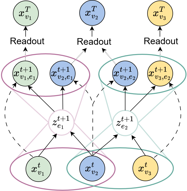
Figure 3: MultiSet layout.

In this Section, we introduce our proposed MultiSet framework, which can be seen as an extension of AllSet where nodes can have multiple co-existing hyperedge–based representations. For a given hyperedge $e\in\mathcal{E}$ in a hypergraph $\mathcal{G}=(\mathcal{V},\mathcal{E})$, we denote by $\bm{z}_{e}^{(t)}\in\mathbb{R}^{d}$ its vector representation at step $t$. For a node $v\in\mathcal{V}$, MultiSet allows for as many representations of the node as the number of hyperedges it belongs to. We denote by $\bm{x}_{v,e}^{(t)}\in\mathbb{R}^{f}$ the vector representation of node $v$ in a hyperedge $e\in\mathcal{E}_{v}$ at propagation time $t$, and by $\mathbb{X}_{v}^{(t)}=\{\bm{x}_{v,e}^{(t)}\}_{e\in\mathcal{E}_{v}}$ the set of all $d_{v}$ hidden states of that node in the specified time-step. Accordingly, the hyperedge and node update rules of MultiSet are formulated to accommodate hyperedge–dependent node representations:

$$\bm{z}_{e}^{(t+1)}=f_{\mathcal{V}\rightarrow\mathcal{E}}(\{\mathbb{X}_{u}^{(t)}\}_{u:u\in e};\bm{z}_{e}^{(t)}),$$ (8)

$$\bm{x}_{v,e}^{(t+1)}=f_{\mathcal{E}\rightarrow\mathcal{V}}(\{\bm{z}_{e}^{(t+1)}\}_{e\in\mathcal{E}_{v}};\{\mathbb{X}_{v}^{(k)}\}_{k=0}^{t}),$$ (9)

where $f_{\mathcal{V}\rightarrow\mathcal{E}}$ and $f_{\mathcal{E}\rightarrow\mathcal{V}}$ are two multiset functions with respect to their first input. After $T$ iterations of message passing, MultiSet also considers a last readout-based step to obtain a unique final representation $\bm{x}_{v}^{T}\in\mathbb{R}^{f^{\prime}}$ for each node from the set of its hyperedge–based representations:

$$\bm{x}_{v}^{(T)}=f_{\mathcal{V}\rightarrow\mathcal{V}}(\{\mathbb{X}_{v}^{(k)}\}_{k=0}^{T})$$ (10)

where $f_{\mathcal{V}\rightarrow\mathcal{V}}$ is also a multiset function.

As we show in the following propositions (proofs can be found in Appendices E and F), both AllSet framework and the more recent EDHNN architecture (Wang et al., 2023) can be expressed in terms of the general MultiSet notation.

Proposition 4.2.

AllSet 5-6, as well as its extension 5-7, are special cases of MultiSet 8-9-10.

Proposition 4.3.

EDHNN (Wang et al., 2023) is a special case of MultiSet 8-9-10.

4.3 Training MultiSet Networks

This section describes the main characteristics of our MultiSet layer implementation, MultiSetMixer, and presents a novel sampling procedure that our model incorporates.

Table 1: Hypergraph model performance benchmarks. Test accuracy in % averaged over 15 splits.

Model Cora Citeseer Pubmed CORA-CA DBLP-CA Mushroom NTU2012 ModelNet40 20Newsgroups ZOO avg. ranking AllDeepSets 77.11 ± 1.00 70.67 ± 1.42 89.04 ± 0.45 82.23 ± 1.46 91.34 ± 0.27 99.96 ± 0.05 86.49 ± 1.86 96.70 ± 0.25 81.19 ± 0.49 89.10 ± 7.00 6.80 AllSetTransformer 79.54 ± 1.02 72.52 ± 0.88 88.74 ± 0.51 84.43 ± 1.14 91.61 ± 0.19 99.95 ± 0.05 88.22 ± 1.42 98.00 ± 0.12 81.59 ± 0.59 91.03 ± 7.31 3.25 UniGCNII 78.46 ± 1.14 73.05 ± 1.48 88.07 ± 0.47 83.92 ± 1.02 91.56 ± 0.18 99.89 ± 0.07 88.24 ± 1.56 97.84 ± 0.16 81.16 ± 0.49 89.61 ± 8.09 4.75 EDHNN 80.74 ± 1.00 73.22 ± 1.14 89.12 ± 0.47 85.17 ± 1.02 91.94 ± 0.23 99.94 ± 0.11 88.04 ± 1.65 97.70 ± 0.19 81.64 ± 0.49 89.49 ± 6.99 2.90 CEGAT 76.53 ± 1.58 71.58 ± 1.11 87.11 ± 0.49 77.50 ± 1.51 88.74 ± 0.31 96.81 ± 1.41 82.27 ± 1.60 92.79 ± 0.44 NA 44.62 ± 9.18 12.11 CEGCN 77.03 ± 1.31 70.87 ± 1.19 87.01 ± 0.62 77.55 ± 1.65 88.12 ± 0.25 94.91 ± 0.44 80.90 ± 1.74 90.04 ± 0.47 NA 49.23 ± 6.81 12.56 HCHA 79.53 ± 1.33 72.57 ± 1.06 86.97 ± 0.55 83.53 ± 1.12 91.21 ± 0.28 98.94 ± 0.54 86.60 ± 1.96 94.50 ± 0.33 80.75 ± 0.53 89.23 ± 6.81 7.85 HGNN 79.53 ± 1.33 72.24 ± 1.08 86.97 ± 0.55 83.45 ± 1.22 91.26 ± 0.26 98.94 ± 0.54 86.71 ± 1.48 94.50 ± 0.33 80.75 ± 0.52 89.23 ± 6.81 7.95 HNHN 77.68 ± 1.08 73.47 ± 1.36 87.88 ± 0.47 78.53 ± 1.15 86.73 ± 0.40 99.97 ± 0.04 88.28 ± 1.50 97.84 ± 0.15 81.53 ± 0.55 89.23 ± 7.85 5.55 HyperGCN 74.78 ± 1.11 66.06 ± 1.58 82.32 ± 0.62 77.48 ± 1.14 86.07 ± 3.32 69.51 ± 4.98 47.65 ± 5.01 46.10 ± 7.95 80.84 ± 0.49 51.54 ± 9.88 14.30 HAN 80.73 ± 1.37 73.69 ± 0.95 86.34 ± 0.61 84.19 ± 0.81 91.10 ± 0.20 91.33 ± 0.91 83.78 ± 1.75 93.85 ± 0.33 79.67 ± 0.55 80.26 ± 6.42 8.90 HAN minibatch 80.24 ± 2.17 73.55 ± 1.13 85.41 ± 2.32 82.04 ± 2.56 90.52 ± 0.50 93.87 ± 1.04 80.62 ± 2.00 92.06 ± 0.63 79.76 ± 0.56 70.39 ± 11.29 10.60 MultiSetMixer 78.06 ± 1.24 71.85 ± 1.50 87.19 ± 0.53 82.74 ± 1.23 90.68 ± 0.19 99.58 ± 0.16 88.90 ± 1.30 98.38 ± 0.21 88.57 ± 1.96 88.08 ± 8.04 6.20 MLP CB 74.06 ± 1.26 71.93 ± 1.53 85.83 ± 0.51 74.39 ± 1.40 84.91 ± 0.44 99.93 ± 0.08 85.43 ± 1.51 96.41 ± 0.32 86.13 ± 2.82 81.61 ± 10.98 10.30 MLP 73.27 ± 1.09 72.07 ± 1.65 87.13 ± 0.49 73.27 ± 1.09 84.77 ± 0.41 99.91 ± 0.08 79.70 ± 1.56 95.31 ± 0.28 80.93 ± 0.59 85.13 ± 6.90 11.50 Transformer 74.15 ± 1.17 71.82 ± 1.51 87.37 ± 0.49 73.61 ± 1.55 85.26 ± 0.38 99.95 ± 0.08 82.88 ± 1.93 96.29 ± 0.29 81.17 ± 0.54 88.72 ± 10.25 9.85

Learning MultiSet layers.

Following the mixer-style block designs (Tolstikhin et al., 2021) and standard practice, we propose the following MultiSet layer implementation:

$$\bm{z}_{e}^{(t+1)} =f_{\mathcal{V}\rightarrow\mathcal{E}}(\{\bm{x}_{u,e}^{(t)}\}_{u:u\in e};\bm{z}_{e}^{(t)})$$ (11)

$$:=\frac{1}{|e|}\sum_{v\in e}\bm{x}^{(t)}_{u,e}+\text{MLP}\left(\text{LN}\left(\frac{1}{|e|}\sum_{v\in e}\bm{x}^{(t)}_{u,e}\right)\right),$$

$$\bm{x}_{v,e}^{(t+1)} =f_{\mathcal{E}\rightarrow\mathcal{V}}(\bm{z}_{e}^{(t+1)};\bm{x}_{v,e}^{(t)})$$ (12)

$$:=\bm{x}_{v,e}^{(t)}+\text{MLP}\left(\text{LN}(\bm{x}_{v,e}^{(t)})\right)+\bm{z}_{e}^{(t+1)},$$

$$\bm{x}_{v}^{(T)} =f_{\mathcal{V}\rightarrow\mathcal{V}}(\mathbb{X}_{v}^{(T)}):=\frac{1}{d_{v}}\sum_{e\in\mathcal{E}_{v}}\bm{x}^{(t)}_{v,e}$$ (13)

where MLPs are composed of two fully-connected layers, and LN stands for layer normalization. This novel architecture, which we call MultiSetMixer, is based on a mixer-based pooling operation for (i) updating hyperedges from its node’s representations, and (ii) generate and update hyperedge-dependent representations of the nodes.

Proposition 4.4.

The functions $f_{\mathcal{V}\rightarrow\mathcal{E}}$, $f_{\mathcal{E}\rightarrow\mathcal{V}}$ and $f_{\mathcal{V}\rightarrow\mathcal{V}}$ defined in MultiSetMixer are permutation invariant. Furthermore, these functions are universal approximators of multiset functions when the size of the input multiset is finite.

Mini-batching.

The motivation for introducing a new strategy to iterate over hypergraph datasets is twofold. On the one hand, current HNN pipelines suffer from scalability issues to process large datasets and immense hyperedges. On the other, pooling operations over relatively large sets can also lead to over-squashing the signal. To help in these directions, we propose sampling $X$ mini-batches of a certain size $B$ at each iteration. At step 1, we sample $B$ hyperedges from $\mathcal{E}$. The hyperedge sampling over $\mathcal{E}$ can be either uniform or weighted (e.g. by taking into account hyperedge cardinalities). Then in step 2 $L$ nodes are in turn sampled from each sampled hyperedge $e$, padding the hyperedge with $L-|e|$ special padding tokens if $|e|<L$ –consisting of $\bm{0}$ vectors that can be easily discarded in some computations. Overall, the shape of the obtained mini-batch $X$ is $B\times L$. Please refer to Appendix L for additional analysis.

5 Experimental Results

The questions that we introduced in the Introduction have shaped our research, leading to a new definition of higher-order homophily and unexplored architectural designs that can potentially fit better the properties of hypergraph networks. In subsequent subsections, we set four questions that follow up from these fundamental inquiries and can help contextualize the technical contributions of this paper.

Datasets and models.

We use the same datasets used in Chien et al. (2022), which includes Cora, Citeseer, Pubmed, ModelNet40, NTU2012, 20Newsgroups, Mushroom, ZOO, CORA-CA, and DBLP-CA. More information about datasets and corresponding statistics are in Appendix H.2. We also utilize the benchmark implementation provided by Chien et al. (2022) to conduct the experiments with several models, including AllDeepSets, AllSetTransformer, EDHNN, UniGCNII, CEGAT, CEGCN, HCHA, HNN, HNHN, HyperGCN, HAN, and HAN mini-batching. Additionally, we consider vanilla MLP applied to node features and a transformer architecture, as well as introduce MultiSetMixer and a new MLP baseline leveraging Connectivity Batching (MLP CB). We refer to Section 4.3 for more details about all these architectures. All models are optimized using 15 splits with 2 model initializations, resulting in a total of 30 runs; see Appendix H.1 for further details.

5.1 How does MultiSetMixer perform?

Our first experiment directly targets our fundamental Q2 by assessing the performance of our proposed MultiSetMixer pipeline together with the other models and baselines. Figure 4 shows the average rankings –across all models and datasets– of the top-5 best-performing models for different training splits, exhibiting that those splits can impact the relative performance among models. However, due to space limitations, we restrict our analysis to the $50\%$ split results shown in Table 1, and relegate to Appendix I.1 the corresponding tables for the other scenarios. Table 1 emphasizes MultiSetMixer solid performance, obtaining the highest test accuracy on NTU2012, ModelNet40, and 20Newsgroups datasets. Notably, MultiSetMixer and MLP CB share similar patterns (see Section 5.3), and both significantly outperform all the other architectures on 20Newsgroup.

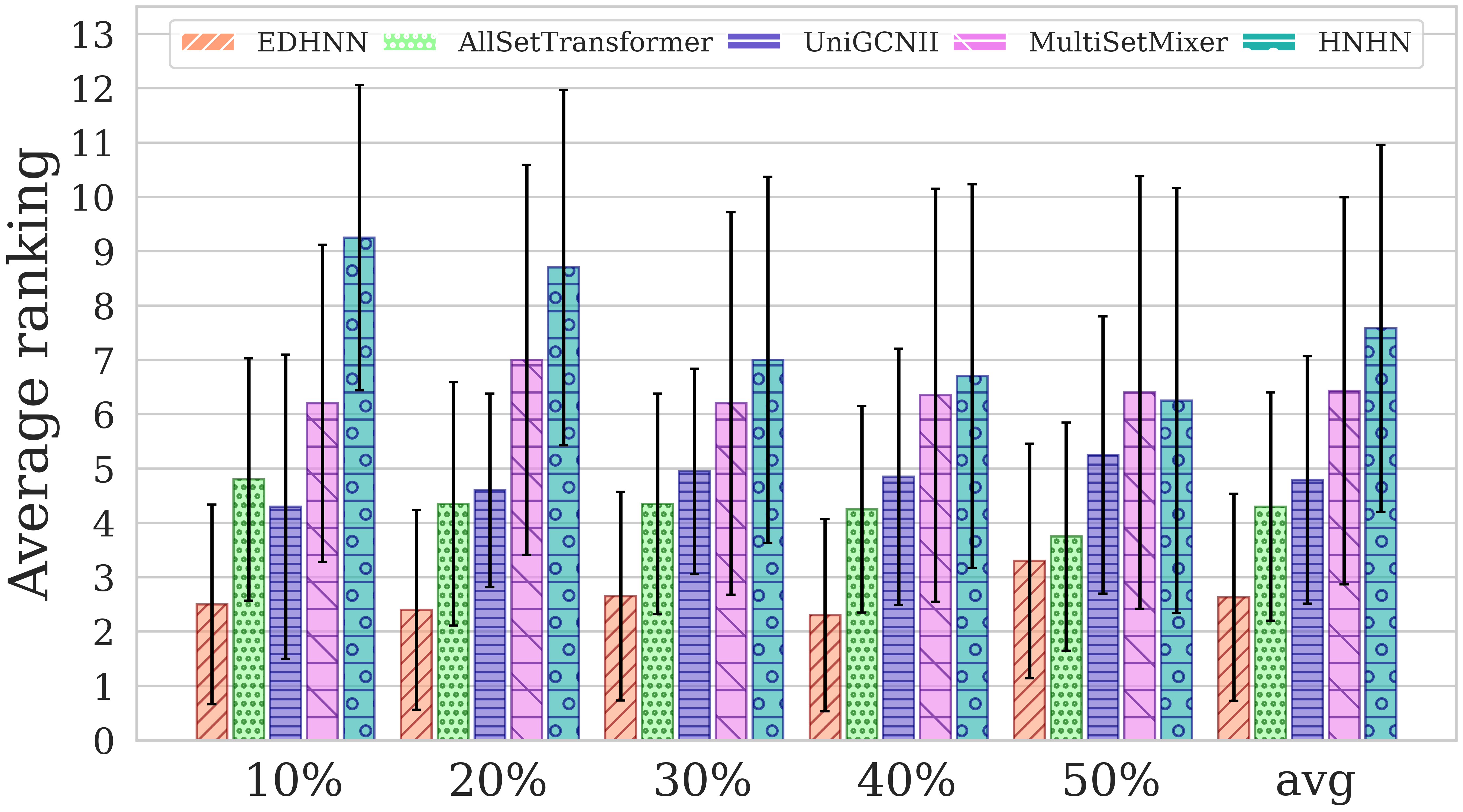
Figure 4: Average rankings and standard deviations at different training percentages, with overall average performance.

In fact, the comparable performance among the rest of HNN models on this dataset suggests that existing architectures can not account for the dataset connectivity. According to what we observed in the qualitative homophily analysis performed in Section 3, 20Newsgroup is densely interconnected, making it highly heterophilic as the MP evolves; we argue this presents a challenge for most of current HNNs architectures. In contrast, CORA-CA exhibits a high degree of homophily within its hyperedges and shows the most significant performance gap between HNNs and the baselines. A similar trend is observed for DBLP-CA (see node homophily plot in Appendix M). Please refer to Section 5.4 for more experiments on the impact of connectivity.

Finally, we highlight the overall good performance obtained by the non-inductive baselines (MLP, MLP CB) in most datasets: only in 3 out of 10 (Cora, CORA-CA, DBLP-CA) HNN architectures significantly outperform all of them. This fact showcases that, so far, features are being more representative than connectivity in most considered hypergraph datasets –a relevant insight for Q3.

Figure 5: Joint visualization of rank dependencies, showing Norm. Acc. versus $\Delta$ Homophily (Eq. 4 at step $t=1$ and $\mu=0.1$) and CE Homophily (Wang et al., 2023). Norm. Acc. (Eq. 14) is assessed for various instances of model A (specified in column titles), with model B being MLP CB. Both axes represent rank values, with lower values indicating better metrics. Arrows denote the rank shift in homophily between CE homophily and $\Delta$ homophily for each dataset.

5.2 When are HNNs exploiting the connectivity?

Motivated by the previous observation of the general results, in this section, we investigate when HNN models actually take advantage of the inductive bias. To do so, we first propose a way to capture the influence of the bias in the downstream task performance –in an attempt to decouple it from the impact of just the dataset features–, and then investigate if the datasets’ homophily scores are able to account for the resulting observations. We argue this study provides a valuable contribution to questions Q2 and Q3.

In order to quantitatively assess the impact of inductive bias, we compare the results of HNNs –i.e., model $A$–, with those of another architecture that does not leverage the connectivity –i.e. a non-inductive baseline, model $B$. Specifically, we measure the difference between the accuracy of model $A$ ($acc_{A}$) and $B$ ($acc_{B}$) (Table 14 in Appendix shows the computed differences considering MLP and MLP CB as baselines). The real-world datasets employed in this study span diverse domains and, as depicted in Table 1, this implies considerable variations in performance values across datasets. In order to mitigate such variability, we introduce the following normalized accuracy relative to $acc_{B}$:

$$\text{Norm. Acc.}=({acc}_{A}-{acc}_{B})/(100-{acc}_{B}).$$ (14)

Next, we are interested in assessing if dataset’s homophily can shed some light on the resulting normalized accuracy measurements. To that end, we consider two different homophily measures: on the one hand, our proposed $\Delta$ homophily between the two first steps of the MP (Eq 4 with $t=1$ and $\mu=0.1$). On the other hand, Clique Expansion (CE) homophily, calculated over the clique expansion of the hypergraph following the approach of Wang et al. (2023). Figure 5 illustrates the rank dependency of normalized accuracy against these two homophily measures, with MLP CB as the non-inductive baseline (as it’s the strongest baseline according to Table 1). Additionally, we show the ideal correlation –performance directly proportional to homophily– with the dashed diagonal, as well as the rank shift in homophily between the two homophily measures through the arrows. The difference between EDHNN, MultiSetMixer, and AllSetTransformer lies in the way message passing propagates information (see Section 4.2). Mushroom and Zoo datasets were excluded due to Mushroom’s discriminatory node features and Zoo’s small hypernetwork size.

The comparison between CE homophily and $\Delta$ homophily reveals a notable trend, with $\Delta$ homophily consistently aligning closer, on average, to the middle dashed line –indicating a higher positive correlation between performance and $\Delta$ homophily level in comparison to CE homophily. Remarkably, across all architectures, the highest normalized accuracy is consistently distributed across ModelNet40, DBLP-CA, and CORA-CA, with $\Delta$ homophily ranking them as the top three accordingly. A striking shift in rankings is observed for the Pubmed dataset, transitioning from the most homophilic under the CE homophily measure to the least homophilic under $\Delta$ homophily. We associate this to the high percentage of isolated nodes ($80.52\%$, see Table 4): while CE homophily scores are largely influenced by them, our proposed measure ignores self-connections. Additionally, the 20Newsgroup dataset occupies the last positions in both homophily ranks, aligning with our quantitative analysis findings.

In summary, we show the applicability of $\Delta$ homophily by showing that it exhibits a positive correlation with respect to the ability of exploiting the connectivity by HNN architectures, significantly stronger than the CE homophily that is commonly used nowadays. Our findings underscore the crucial role of accurately expressing homophily in hypergraph networks, entangling with the complexity in capturing higher-order dependencies.

5.3 What is the impact of the mini-batch sampling?

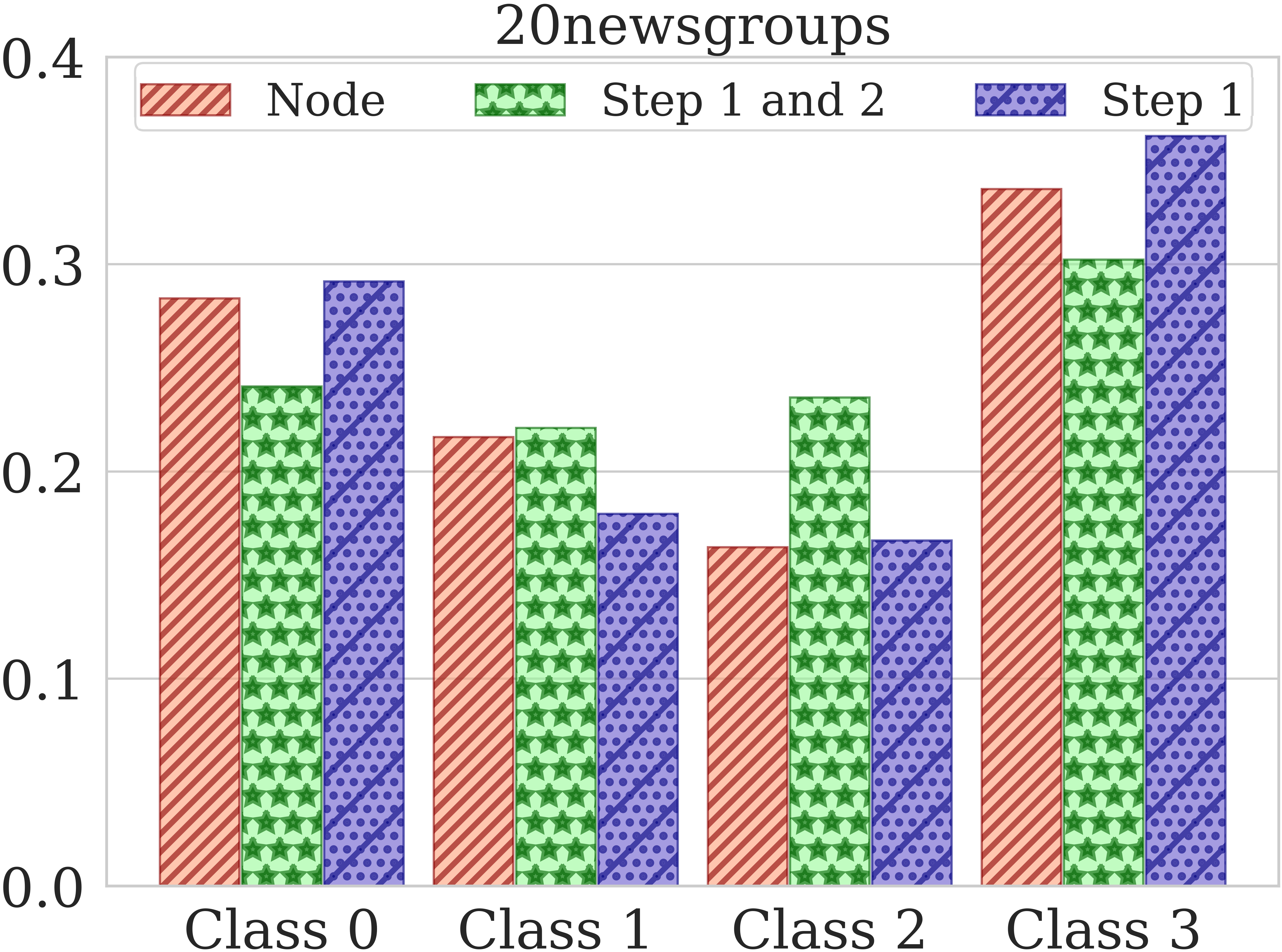
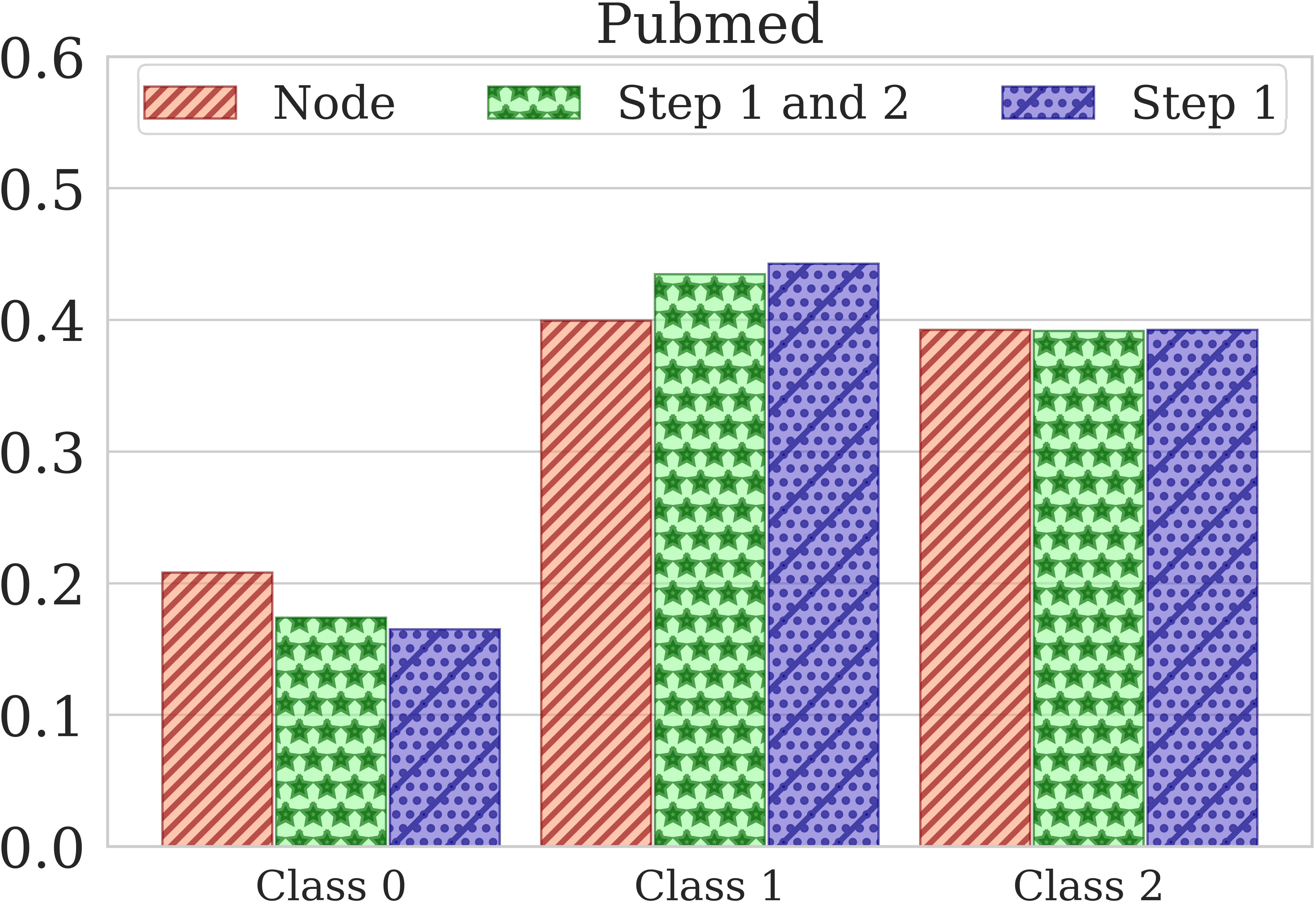
Figure 6: Class distribution shift induced by mini-batching: ‘Node’ represents the original node class distribution, ‘Step 1 and 2’ the resulting one after sampling both hyperedges and nodes, and ‘Step 1’ when only sampling hyperedges.

Next, we examine the role of our proposed mini-batching sampling in explaining the general results shown in Table 1, and investigate how it influences other models’ performance. These experiments provide valuable insights on Q2.

Table 2: Mini-batching experiment. Test accuracy in % averaged over 15 splits.

Model Cora Citeseer Pubmed CORA-CA DBLP-CA Mushroom NTU2012 ModelNet40 20Newsgroups ZOO avg. ranking AllSetTransformer (batched) 74.34 ± 1.08 69.67 ± 1.46 87.75 ± 0.30 75.75 ± 1.46 86.06 ± 0.22 99.91 ± 0.05 87.55 ± 0.86 96.42 ± 0.17 81.37 ± 0.28 93.20 ± 5.38 2.70 EDHNN 77.88 ± 0.69 69.51 ± 0.87 86.82 ± 0.33 83.12 ± 0.89 90.45 ± 0.28 99.95 ± 0.04 87.64 ± 0.99 97.55 ± 0.17 81.23 ± 0.31 90.00 ± 4.43 2.40 MultiSetMixer 78.06 ± 1.24 71.85 ± 1.50 87.19 ± 0.53 82.74 ± 1.23 90.68 ± 0.19 99.58 ± 0.16 88.90 ± 1.30 98.38 ± 0.21 88.57 ± 1.96 88.08 ± 8.04 1.80 HAN minibatch 80.24 ± 2.17 73.55 ± 1.13 85.41 ± 2.32 82.04 ± 2.56 90.52 ± 0.50 93.87 ± 1.04 80.62 ± 2.00 92.06 ± 0.63 79.76 ± 0.56 70.39 ± 11.29 3.10

Class distribution analysis.

To evaluate and motivate the potential of the proposed mini-batching sampling, we investigate the reason behind both (i) the superior performance of MultiSetMixer and MLP CB on 20NewsGroup, NTU2012, ModelNet40, and (ii) their poor performance on Pubmed. Framing mini-batching from the connectivity perspective presents a challenge that conceals significant potential for improvement (Teney et al., 2023). It is important to note that connectivity, by definition, describes relationships among the nodes, implying that some parts of the dataset might interconnect more densely, creating some sort of hubs within the network. Thus, mini-batching might introduce unexpected skew in training distribution. In particular, Figure 6, depicts the original class distribution of the dataset, and compares it to the skewed distributions resulting from employing the corresponding steps of mini-batching (see Section 4.3). Note that, when sampling both hyperedges and nodes (‘Step 1 and 2’), dominant classes 0 and 3 undergo undersampled, contributing to a more balanced distribution in the case of 20Newsgroup. Conversely, for Pubmed, class 2 is undersampled, while the predominant 1st class experiences oversampling, further skewing the distribution in this dataset. This observation leads to the hypothesis that, in some cases, the sampling procedure produces a natural shift that rebalances the class distributions, which in turn helps to improve the performance.

Application to other models.

Furthermore, we explore the proposed mini-batch sampling procedure with the AllSetTransformer and EDHNN models by just sampling hyperedges without additional hyperparameter optimization. From Table 2, we can observe a drop in performance for most of the datasets both for AllSetTransformer and for EDHNN, but overall they in turn outperform the HAN (mini-batching) model. This suggests the substantial potential of the proposed sampling procedure.

5.4 How do connectivity changes affect performance?

Two experimental approaches are designed to systematically alter the original connectivity of datasets. The first setting involves removing hyperedges through various drop connectivity strategies, and the results show that retaining 25% of the largest hyperedges in the Cora, CORA-CA, and DBLP-CA datasets is sufficient to achieve performance comparable to the original connectivity. Additionally, the best-performing HNNs tend to ignore connectivity information on Citeseer, Pubmed, 20Newsgroups and Mushroom. Moreover, the CEGAT model shows improvement in performance across 7 out of 9 datasets.

The second set of experiments focuses on preprocessing the hypergraph connectivity by splitting the original hyperedges to obtain more homophilic ones. Two different strategies are considered: in the first one, the original hyperedges are split into fully homophilic ones by partitioning considering node labels. In the second, instead, we partition based on the initial node features using $k$-means within each hyperedge. The former demonstrates that graph-based methods achieve equivalent performance to HNNs under perfect homophilic hyperedges. In contrast, the latter strategy leads to an improvement for CEGCN and affects the distribution shifts for MultiSetMixer.

More details about the drop connectivity and the preprocessing connectivity strategies, as well as a deeper analysis of the corresponding results can be found in Appendix I.2. These findings shed some light on our fundamental questions Q1, Q2 and Q3.

6 Discussion

This last section aims to summarize some key findings from our extensive evaluation that can potentially help in improving future HNN related research. Here, we connect our findings to each of the fundamental questions raised in Section 1, which actually drove our research.

Q1: We show that the introduced message passing homophily measure allows for a deeper understanding of hypernetwork dynamics, and the derived $\delta$ homophily metric showcases a strong correlation with respect to HNN’s ability of exploiting their inductive biases. Overall, we argue that the proposed measures are more meaningful than previous higher-order homophily concepts, potentially helping to further explore new ways of assessing and processing hypernetworks. (Sections 3, 5.2, and Appendix I.2)

Q2: We argue that three main contributions presented in this paper –Message Passing Homophily, MultiSet framework with hyperedge-dependent node representations, MultiSetMixer model with mini-batch sampling– have been directly inspired from natural properties of hypernetworks and higher-order dynamics within them, thus no longer relying on extensions of graph-based approaches. Our experimental findings initiate a compelling discussion on the implications of innovative techniques for processing hypergraph data and defining HNNs. (Sections 4.2,4.3, and Appendix I.2)

Q3: Across our extensive evaluation, our results suggest that the expressive power of node features alone is sufficient for a decent performance in the node classification task execution; the gap between models with inductive bias and without is far shorter than one would expect. Addressing this gap presents an open challenge for future research endeavors, and we posit the necessity for additional benchmark datasets where connectivity plays a pivotal role. (Section 5, and Appendix I.2)

For a more in-depth discussion, please refer to the extended conclusion and discussion in Appendix A.

7 Impact Statement

This paper aims to advance hypergraph learning, enhancing our comprehension of intricate relationships and structures with applications across various disciplines. Our study is particularly relevant to behavioral studies, where hypergraph structures enable more accurate modeling of complex interactions (Han et al., 2023; Sun et al., 2023). Moreover, applications of HGNNs in recommendation systems and personalized services can lead to more accurate and tailored experiences for individuals, improving user satisfaction. The ethical considerations align with well-established concerns in the broader field of Machine Learning rather than being specific to our work. The application of hypergraph neural networks in real-world scenarios may raise ethical considerations, encompassing concerns about fairness, transparency, and the potential amplification and propagation of biases within the training data.

Supplementary Materials

Appendix A Extended Conclusion and Discussion

This section summarizes key findings from our extensive evaluation and proposed frameworks. Here we recap the question and summarize the answers to these questions revealed by this work.

Q1: Can the concept of homophily play a crucial role in HNNs, similar to its significance in graph-based research? We show that the concept of homophily in higher-order networks is considerably more complicated compared to networks that exhibit only pairwise connections. To address the issue, we introduce a novel message passing homophily framework that is capable of characterizing homophily in hypergraphs through the distribution of node features as well as node class distribution. In Section 3, we present $\Delta$ homophily, based on the dynamic nature of the proposed message passing homophily, showing that it correlates better with HNN models’ performance than classical homophily measures over the clique-expanded hypergraph. Our findings underscore the crucial role of accurately expressing homophily in HNNs, emphasizing its complexity and the potential in capturing higher-order dynamics. Moreover, in our experiments (see Appendix I.2.2) we demonstrate that rewiring hyperedges for perfect homophily leads to similar results for graph-based methods (CEGCN, CEGAT) and HNN models. Overall, our findings potentially pave the way for new research directions in hypergraph literature, from defining new dynamic-based homophily measures to develop novel connectivity rewiring techniques.

Q2: Given that current HNNs are predominantly extensions of GNN architectures adapted to the hypergraph domain, are these extended methodologies suitable, or should we explore new strategies tailored specifically for handling hypergraph-based data? The three main contributions presented in this paper –Message Passing Homophily, MultiSet framework with hyperedge-dependent node representations, MultiSetMixer model with mini-batch sampling – have been directly inspired from natural properties of hypernetworks and higher-order dynamics within them, thus no longer relying on extensions of graph-based approaches. Based on our experimental results and analysis, the proposed methodologies open an interesting discussion about the impact of novel ways of processing hypergraph-data and defining HNNs. For instance, our mini-batching sampling strategy –which helps addressing scalability issues of current solutions– allowed us to realize the implicit introduction of node class distribution shifts in the process. This study could potentially lead to the definition of meaningful connectivity rewiring techniques, as we already explore in Section 5.4. Furthermore, we show that the introduced message passing and $\Delta$ homophily measures allows for a deeper understanding of the hypernetwork topology and its correlation to the HNN models’ performances. Overall, and despite also identifying some common failure modes of our proposed methods (Section 5), we argue that these contributions provide a new perspective on dealing and processing higher-order networks that go beyond the graph domain.

Q3: Are the existing hypergraph benchmarking datasets meaningful and representative enough to draw robust and valid conclusions? In Appendices I.2.1 and I.2.2, we demonstrate that the significant performance gap between models and MLP on Cora, CORA-CA, and DBLP-CA is primarily influenced by the largest hyperedge cardinalities. Further analysis using $\Delta$ homophily reveals that their notable improvement is strongly tied to the homophilic nature of the one-hop neighborhood. Additionally, the experimental results in Section 5.1 and 5.4 highlight challenges for current HNNs with certain benchmark hypergraph datasets. Specifically, we find that HNN models ignore connectivity for Citeseer, Pubmed, and 20Newsgroups, as well as for the Mushroom dataset, due to highly discriminative features. Furthermore, we observe that models that do not rely on inductive bias (i.e. do not use connectivity in the architecture), consistently exhibit good performance across the majority of datasets. This suggests that the expressive power of node features alone is sufficient for efficient task execution. Addressing this gap presents an open challenge for future research endeavors, and we posit the necessity for additional benchmark datasets where connectivity plays a pivotal role. In addition to this, we believe it would be also interesting to analyze datasets involving higher-order relationships where node classes explicitly depend on hyperedges, as introduced in Choe et al. (2023).This could represent an insightful line of research to further exploit hyperedge-based node representations.

Appendix B Extended Related Works on Hypergraph Neural Networks

Numerous machine-learning techniques have been developed for processing hypergraph data. One commonly used approach in early literature is to transform the hypergraph into a graph through clique expansion (CE). This technique involves substituting each hyperedge with an edge for every pair of vertices within the hyperedge, creating a graph that can be analyzed using graph-based algorithms (Agarwal et al., 2006; Zhou et al., 2006; Zhang et al., 2018; Li & Milenkovic, 2017).

Several techniques have been proposed that use Hypergraph Neural Networks (HNNs) for semi-supervised learning. One of the earliest methods extends the graph convolution operator by incorporating the normalized hypergraph Laplacian (Feng et al., 2019). As pointed out in Dong et al. (2020), spectral convolution with the normalized Laplacian corresponds to performing a weighted CE of the hypergraph. HyperGCN (Yadati et al., 2019) employs mediators for incomplete CE on the hypergraph, which reduces the number of edges required to represent a hyperedge from a quadratic to a linear number of edges. The information diffusion is then carried out using spectral convolution for hypergraph-based semi-supervised learning. Hypergraph Convolution and Hypergraph Attention (HCHA) (Bai et al., 2021) employs modified degree normalizations and attention weights, with the attention weights depending on node and hyperedge features.

CE may cause the loss of important structural information and result in suboptimal learning performance (Hein et al., 2013; Chien et al., 2022). Furthermore, these models typically obtain the best performance with shallow 2-layer architectures. Adding more layers can lead to reduced performance due to oversmoothing (Huang & Yang, 2021). In the recent study Chen & Zhang (2022), an attempt was made to address oversmoothing in this type of network by incorporating residual connections; however, the method still relies on using hypergraph Laplacians to build a weighted graph through clique expansion. Another method presented in Yang et al. (2020) introduces a new hypergraph expansion called line expansion (LE) that treats vertices and hyperedges equally. The LE bijectively induces a homogeneous structure from the hypergraph by modeling vertex-hyperedge pairs. In addition, the LE and CE techniques require significant computational resources to transform the original hypergraph into a graph and perform subsequent computations, hence making the methods unpractical for large hypergraphs.

Another line of research explores hypergraph modeling involving a two-stage procedure: information is transmitted from nodes to hyperedges and then back from hyperedges to nodes (Wei et al., 2021; Yi & Park, 2020; Dong et al., 2020; Arya et al., 2020; Huang & Yang, 2021; Yadati et al., 2020). This procedure can be viewed as a two-step message passing mechanism. HyperSAGE (Arya et al., 2020) is a prominent early example of this line of research allowing transductive and inductive learning over hypergraphs. Although HyperSAGE has shown improvement in capturing information from hypergraph structures compared to spectral-based methods, it involves only one learnable linear transformation and cannot model arbitrary multiset function (Chien et al., 2022). Moreover, the algorithm utilizes nested loops resulting in inefficient computation and poor parallelism.

UniGNN (Huang & Yang, 2021) addresses some of these limitations by using a permutation-invariant function to aggregate vertex features within each hyperedge in the first stage and using learnable weights only during the second stage to update each vertex with its incident hyperedges. One of the variations of UniGNN, called UniGCNII addresses the oversmoothing problem, which is common for most of the methods described above. It accomplishes this by adapting GCNII (Chen et al., 2020) to hypergraphs. The AllSet method, proposed in Chien et al. (2022), employs a composition of two learnable multiset functions to model hypergraphs. It presents two model variations: the first one exploits Deep Set (Zaheer et al., 2017) and the second one Set Transformer (Lee et al., 2019). The AllSet method can be seen as a generalization of the most commonly used hypergraph HNNs (Yadati et al., 2019; Feng et al., 2019; Bai et al., 2021; Dong et al., 2020; Arya et al., 2020). More implementation details and detailed drawbacks discussion can be found in Section 4.1. Although AllSet achieves state-of-the-art results, it suffers from the drawbacks of the message passing mechanism, including the local receptive field, resulting in a limited ability to model long-range interactions (Gu et al., 2020; Balcilar et al., 2021). Two additional issues are poor scalability to large hypergraph structures and oversmoothing that occurs when multiple layers are stacked.

Finally, we would like to mention two related papers that put the focus on hyperedge-dependent computations. On the one hand, EDHNN (Wang et al., 2023) incorporates the option of hyperedge-dependent messages from hyperedges to nodes; however, at each iteration of the message passing it aggregates all these messages to generate a unique node hidden representation, and thus it doesn’t enable to keep different hyperedge-based node representations across the whole procedure –as our MultiSetMixer does. On the other hand, the work Aponte et al. (2022) does allow multiple hyperedge-based representations across the message passing, but the theoretical formulation of this unpublished paper is not clear and rigorous, and the evaluation is neither reproducible nor comparable to other hypergraph models. Hence, we argue that our MultiSet framework represents a step forward by rigorously formulating a simple but general MP framework for hypergraph modelling that is flexible enough to deal with hyperedge-based node representations and residual connections, demonstrating as well that it generalizes previous hypergraph and graph models.

Appendix C Details of the Implemented Methods

We provide a detailed overview of the models analyzed and tested in this work. In order to make their similarities and differences more evident, we express their update steps through a standard and unified notation.

Notation.

A hypergraph with $n$ nodes and $m$ hyperedges can be represented by an incidence matrix $\bm{H}\in\mathbb{R}^{n\times m}$. If the hyperedge $e_{j}$ is incident to a node $v_{i}$ (meaning $v_{i}\in e_{j}$), the entry in the incidence matrix ${H}_{i,j}$ is set to $1$. Instead, if $v_{i}\notin e_{j}$, then ${H}_{i,j}=0$.

We denote with $\bm{W}$ and $\bm{b}$ a learnable weight matrix and bias of a neural network, respectively. Generally, $\bm{x}_{v}$ and $\bm{z}_{e}$ are used to denote features for a node $v$ and a hyperedge $e$ respectively. Stacking all node features together we obtain the node feature matrix $\bm{X}$, while $\bm{Z}$ is instead the hyperedge feature matrix. $\sigma(\cdot)$ indicates a nonlinear activation function (such as ReLU, ELU or LeakyReLU) that depends on the model used. Finally, we use $\|$ to denote concatenation.

C.1 AllSet-like models

This Section addresses the models that are covered in the AllSet unified framework introduced in 4.1, and that can potentially be expressed as particular instances of equations 5 and 7. For a detailed proof of the claim for most of the following models, refer to Theorem 3.4 in Chien et al. (2022).

CEGCN / CEGAT.

As introduced in the previous Sections, the CE of a hypergraph $\mathcal{G}=(\mathcal{V},\mathcal{E})$ is a weighted graph obtained from $\mathcal{G}$ with the same set of nodes. In terms of incidence matrix, it can be described as $\bm{H}^{(CE)}=\bm{H}\bm{H}^{T}$ (Chien et al., 2022). A one-step update of the node feature matrix $\bm{X}\in\mathbb{R}^{n\times f}$ can be expressed both in a compact way as $\bm{H}^{(CE)}\bm{X}$ or directly as a node-level update rule, as

$$\bm{x}_{v}^{(t+1)}=\sum_{e\in\mathcal{E}_{v}}\sum_{u:u\in e}{\bm{x}_{v}^{(t)}}.$$ (15)

Some types of hypergraph convolutional layers in the literature adopt a CE-based propagation, for example generalizing popular graph-targeting models such as Graph Convolutional Networks (Kipf & Welling, 2017) and Graph Attention Networks (Veličković et al., 2017).

HNN.

Before describing how HNN (Feng et al., 2019) works, it is necessary to define some notation. Let $\bm{H}$ be the hypergraph’s incidence matrix. Suppose that each hyperedge $e\in\mathcal{E}$ is assigned a fixed positive weight $z_{e}$, and let $\bm{Z}\in\mathbb{R}^{m\times m}$ now denote the matrix stacking all these weights in the diagonal entries. Additionally, the vertex degree is defined as

$$d_{v}=\sum_{e\in\mathcal{E}_{v}}z_{e},$$ (16)

while the hyperedge degree, instead, is

$$b_{e}=\sum_{v:v\in e}1.$$ (17)

The degree values can be used to define two diagonal matrices, $\bm{D}\in\mathbb{R}^{n\times n}$ and $\bm{B}\in\mathbb{R}^{m\times m}$.

The core of the hypergraph convolution introduced in Feng et al. (2019) can be expressed as

$$\bm{x}_{v}^{(t+1)}=\sigma\left(\sum_{e\in\mathcal{E}_{v}}\sum_{u:u\in e}z_{e}\bm{x}_{v}^{(t)}\bm{W}^{(t)}\right),$$ (18)

where $\sigma$ is a non-linear activation function like LeakyReLU and ELU, and $\bm{W}^{(t)}\in\mathbb{R}^{f^{(t)}\times f^{(t+1)}}$ is a weight matrix between the $(t)$-th and $(t+1)$-th layer, to be learnt during training. Note that in this case the dimensionality of the node feature vectors $f^{(t)}$ can be layer-dependent.

The update step can be rewritten also in matrix form as

$$\bm{X}^{(t+1)}=\sigma(\bm{H}\bm{Z}\bm{H}^{T}\bm{X}^{(t)}\bm{W}^{(t)}),$$ (19)

where $\bm{X}^{(t+1)}\in\mathbb{R}^{n\times f^{(t+1)}}$ and $\bm{X}^{(t)}\in\mathbb{R}^{n\times f^{(t)}}$.

In practice, a normalized version of this update procedure is proposed. The matrix-based formulation allows to clearly express the symmetric normalization that is actually put in place through the vertex and hyperedge degree matrices $\bm{D}$ and $\bm{B}$ defined above:

$$\bm{X}^{(t+1)}=\sigma(\bm{D}^{-1/2}\bm{H}\bm{Z}\bm{B}^{-1}\bm{H}^{T}\bm{D}^{-1/2}\bm{X}^{(t)}\bm{W}^{(t)}).$$ (20)

HCHA.

With respect to the previously described models, HCHA (Bai et al., 2021) uses a different kind of weights that depend on the node and hyperedge features. Specifically, starting from the same convolutional model proposed by Feng et al. (2019) and described in Equation 20, they explore the idea of introducing an attention learning model on $\bm{H}$.

Their starting point is the intuition that hypergraph convolution as implemented in Equation 20 implicitly puts in place some attention mechanism, which derives from the fact that the afferent and efferent information flow to vertexes may be assigned different importance levels, which are statically encoded in the incidence matrix $\bm{H}$, hence depend only on the graph structure. In order to allow for such information on magnitude of importance to be determined dynamically and possibly vary from layer to layer, they introduce an attention learning module on the incidence matrix $\bm{H}$: instead of maintaining $\bm{H}$ as a binary matrix with predefined and fixed entries depending on the hypergraph connectivity, they suggest that its entries could be learnt during the training process. The entries of the matrix should express a probability distribution describing the degree of node-hyperedge connectivity, through non-binary and real values.

Nevertheless, the proposed hypergraph attention is only feasible when the hyperedge and vertex sets share the same homogeneous domain, otherwise, their similarities would not be compatible. In case the comparison is feasible, the computation of attention scores is inspired by (Veličković et al., 2017): for a given vertex $v$ and a hyperedge $e$, the score is computed as

$${H}_{v,e}=\frac{\mathrm{exp}(\sigma(\mathrm{sim}(\bm{x}_{v}\bm{W},\bm{z}_{e}\bm{W})))}{\sum_{g\in\mathcal{E}_{v}}\mathrm{exp}(\sigma(\mathrm{sim}(\bm{x}_{v}\bm{W},\bm{z}_{g}\bm{W})))},$$ (21)

where $\sigma$ is a non-linear activation function, and sim is a similarity function defined as

$$\mathrm{sim}(\bm{x}_{v},\bm{z}_{e})=\bm{a}^{T}[\bm{x}_{v}\mathbin{\|}\bm{z}_{e}],$$ (22)

in which $\bm{a}$ is a weight vector, and the resulting similarity value is a scalar.

HyperGCN.

The method proposed by Yadati et al. (2019) can be described as performing two steps sequentially: first, a graph structure is defined starting from the input hypergraph, through a particular procedure, and then the well known CGN model (Kipf & Welling, 2017) for standard graph structures is executed on it. Depending on the approach followed in the first step, three slight variations of the same model can be identified: 1-HyperGCN, HyperGCN (enhancing 1-HyperGCN with so-called mediators) and FastHyperGCN.

Before analyzing the differences among the three techniques, we introduce some notation and express how the GCN-update step is performed. Suppose that the input hypergraph $\mathcal{G}=(\mathcal{V,\mathcal{E}})$ is equipped with initial edge weights $\{z_{e}\}_{e\in\mathcal{E}}$ and node features $\{\bm{x}_{v}\}_{v\in\mathcal{V}}$ (if missing, suppose to initialize them randomly or with constant values). Let $\bm{\bar{A}}^{(t)}$ denote the normalized adjacency matrix associated to the graph structure at time-step $(t)$. The node-level one-step update for a specific node $v$ can be formalized as:

$$\bm{x}_{v}^{(t+1)}=\sigma\left(\left(\bm{W}^{(t)}\right)^{T}\sum_{u\in\mathcal{N}_{v}}{{\bar{A}}^{(t)}_{u,v}\cdot\bm{x}_{u}^{(t)}}\right),$$ (23)

in which $\bm{x}_{v}^{(t+1)}$ is the $(t+1)$-th step hidden representation of node $v$ and $\mathcal{N}_{v}$ is the set of neighbors of $v$. For what concerns ${\bar{A}}^{(t)}_{u,v}$, it refers to the element at index $u,v$ of ${\bm{\bar{A}}}^{(t)}$, which can be defined in the following ways according to the method:

1. 1-HyperGCN: starting from the hypergraph $\mathcal{G}=(\mathcal{V,\mathcal{E}})$, a simple graph is defined by considering exactly one representative simple edge for each hyperedge $e\in\mathcal{E}$, and it is defined as $(v_{e},u_{e})$ such that $(v_{e},u_{e})=\mathrm{argmax}_{v,u\in e}{\lVert\left(\bm{W}^{(t)}\right)^{T}(\bm{x}_{v}^{(t)}-\bm{x}_{u}^{(t)})\rVert_{2}}$. This implies that each hyperedge $e$ is represented by just one pairwise edge $(v_{e},u_{e})$, and this may also change from one step to the other, which leads to the graph adjacency matrix ${\bm{\bar{A}}}^{(t)}$ being layer-dependent, too.

2. HyperGCN: the model extends the graph construction procedure of 1-HyperGCN by also considering mediator nodes, that for each hyperedge $e$ consist in $K_{e}:=\{k\in e:k\neq v_{e},k\neq u_{e}\}$. Once the representative edge $(v_{e},u_{e})$ is determined and added to the newly defined graph, two edges for each mediator are also introduced, connecting the mediator to both $v_{e}$ and $u_{e}$. Because there are $2|e|-3$ edges for each hyperedge $e$, each weight is chosen to be $\frac{1}{2|e|-3}$ in order for the weights in each hyperedge to sum to 1. The generalized Laplacian obtained this way satisfies all the properties of the HyperGCN’s Laplacian (Yadati et al., 2019).

3. FastHyperGCN: in order to save training time, in this case the adjacency matrix ${\bm{\bar{A}}}^{(t)}$ is computed only once before training, by using only the initial node features of the input hypergraph.

UniGCNII.

This model aims to extend to hypergraph structures the GCNII model proposed by Chen et al. (2020) for simple graph structures, that is a deep graph convolutional network that puts in place an initial residual connection and identity mapping as a way to reduce the oversmoothing problem (Huang & Yang, 2021).

Let $d_{v}$ denote the degree of vertex $v$, while $d_{e}=\frac{1}{|e|}\sum_{i\in e}{d_{i}}$ for each hyperedge $e\in\mathcal{E}$. A single node-level update step performed by UniGCNII can be expressed as:

$$\bm{\hat{x}}_{v}^{(t)}=\frac{1}{\sqrt{d_{v}}}\sum_{e\in\mathcal{E}_{v}}\frac{\bm{z}_{e}^{(t)}}{\sqrt{d_{e}}},$$ (24)

$$\bm{{x}}_{v}^{(t+1)}=((1-\beta)\bm{I}+\beta\bm{W}^{(t)})((1-\alpha)\bm{\hat{x}}_{v}^{(t)}+\alpha\bm{{x}}_{v}^{(0)}).$$ (25)

in which $\alpha$ and $\beta$ are hyperparameters, $\bm{I}$ is identity matrix and $\bm{{x}}_{v}^{(0)}$ is the initial feature of vertex $i$.

HNHN.

For the HNHN model by Dong et al. (2020), hypernode and hyperedge features are supposed to share the same dimensionality $d$, hence in this case $\bm{X}\in\mathbb{R}^{n\times d}$ and $\bm{Z}\in\mathbb{R}^{m\times d}$. The update rule in this case can be easily expressed using the incidence matrix as

$$\bm{Z}^{(t+1)}=\sigma(\bm{H}^{T}\bm{X}^{(t)}\bm{W}_{Z}+\bm{b_{Z}}),$$ (26)

$$\bm{X}^{(t+1)}=\sigma(\bm{H}\bm{Z}^{(t+1)}\bm{W}_{X}+\bm{b_{X}}).$$ (27)

in which $\sigma$ is a nonlinear activation function, $\bm{W}_{X},\bm{W}_{Z}\in\mathbb{R}^{d\times d}$ are weight matrices, and $\bm{b_{X}},\bm{b_{Z}}\in\mathbb{R}^{d}$ are bias terms.

AllSet.

The general formulation for the propagation setting of AllSet (Chien et al., 2022) is introduced in Subsection 4.1 and, starting from that, we now analyze the different instances of the model obtained by imposing specific design choices in the general framework.

In the practical implementation of the model, the update functions $f_{\mathcal{V}\rightarrow\mathcal{E}}$ and $f_{\mathcal{E}\rightarrow\mathcal{V}}$, that are required to be permutation invariant with respect to their first input, are parametrized and learnt for each dataset and task. Furthermore, the information of their second argument is not utilized in practice, hence their input can be more generally denoted as a set $\mathbb{S}$.

The two architectures AllDeepSets and AllSetTransformer are obtained in the following way, depending on whether the update functions are defined either as MLPs or Transformers:

1. AllDeepSets (Chien et al., 2022): $f_{\mathcal{V}\rightarrow\mathcal{E}}(\mathbb{S})=f_{\mathcal{E}\rightarrow\mathcal{V}}(\mathbb{S})=\mathrm{MLP}(\sum_{s\in\mathbb{S}}{\mathrm{MLP}(s)})$;

2. AllSetTransformer (Chien et al., 2022), in which the update functions are defined iteratively through multiple steps as they were first designed by Vaswani et al. (2017).

   The first set of operations corresponds to the self-attention module. Suppose that $h$ attention heads are considered: first of all, $h$ pairs of matrices $\bm{K}_{i}$ (keys) and $\bm{V}_{i}$ (values) with $i\in\{1,...,h\}$ are computed from the input set through different MLPs. Additionally, $h$ weights $\theta_{i},i\in\{1,...,h\}$ are also learned and together with the keys and values they allow for the computation of each head-specific attention value $\bm{O}_{i}$ using an activation function $\omega$ (Vaswani et al., 2017). The $h$ attention heads are processed in parallel and they are then concatenated, leading to a unique vector being the result of the multi-head attention module $\mathrm{MH}_{h,\omega}$. After that, a sum operation and a Layer Normalization (LN) (Ba et al., 2016) are applied:

   $$\bm{K}_{i}=\text{MLP}^{K}_{i}(\mathbb{S}),\bm{V}_{i}=\text{MLP}^{V}_{i}(\mathbb{S}),\quad\text{where}\quad i\in\{1,...,h\},$$ (28)

   $$\theta\overset{\Delta}{=}\mathbin{\|}_{i=1}^{h}\theta_{i},$$ (29)

   $$\bm{O}_{i}=\omega(\theta_{i}(\bm{K}_{i})^{T})\bm{V}_{i},\quad\text{where}\quad i\in\{1,...,h\},$$ (30)

   $$\text{MH}_{h,\omega}(\theta,\mathbb{S},\mathbb{S})=\mathbin{\|}_{i=1}^{h}\bm{O}^{(i)},$$ (31)

   $$\bm{Y}=\text{LN}(\theta+\text{MH}_{h,\omega}(\theta,\mathbb{S},\mathbb{S})).$$ (32)

   A feed-forward module follows the self-attention computations, in which a MLP is applied to the feature matrix and then sum and LN are performed again, corresponding to the last operations to be performed:

   $$f_{\mathcal{V}\rightarrow\mathcal{E}}(\mathbb{S})=f_{\mathcal{E}\rightarrow\mathcal{V}}(\mathbb{S})=\text{LN}(\bm{Y}+\text{MLP}(\bm{Y})).$$ (33)

C.2 Other models

This Section describes the models that are considered for the experiments but that don’t fall directly under the AllSet unified framework defined in Section 4.1.

EDHNN.

The Equivariant Diffusion-based HNN model, shortened as EDHNN (Wang et al., 2023) represents the first attempt to draw a connection between the class of hypergraph diffusion algorithms and the design of Hypergraph Neural Networks. The underlying motivation is that, by enabling the model to approximate any continuous equivariant hypergraph diffusion operator, a broad spectrum of higher-order relations can be encoded.

In EDHNN, the hypergraph diffusion operators are learned directly from data, harnessing the expressive power of Neural Networks. This leads to the development of a novel Hypergraph Neural Network inspired by hypergraph diffusion solvers, with the subsequent operations executed at each layer described in the following.

The hyperedge-level feature update is performed as

$$\bm{z}_{e}^{(t+1)}=\sum_{u\in e}\hat{\phi}(\bm{x}_{u}^{(t)}),$$ (34)

and starting from that, the node-level update is defined as

$$\bm{x}_{v}^{(t+1)}=\hat{\psi}\left(\bm{x}_{v}^{(t)},\sum_{e\in\mathcal{E}_{v}}\hat{\rho}(\bm{x}_{v}^{(t)},\bm{z}_{e}^{(t+1)}),\bm{x}_{v}^{0},d_{v}\right).$$ (35)

In the equations above, $\hat{\psi}$, $\hat{\phi}$ and $\hat{\rho}$ are three MLPs shared across layers.

HAN.

The Heterogeneous Graph Attention Network model (Wang et al., 2019) is specifically designed for processing and performing inference on heterogeneous graphs. Heterogeneous graphs have various types of nodes and/or edges, and standard GNN models that treat all of them equally are not able to properly handle such complex information.

In order to apply this model on hypergraphs, (Chien et al., 2022) define a preprocessing step to derive a heterogeneous graph from a hypergraph. Specifically, a bipartite graph is defined such that there is a bijection between its nodes and the set of nodes and hyperedges in the original hypergraph. The nodes obtained in this way belong to one of two distinct types, that are the sets $\mathbb{V}$ and $\mathbb{E}$ (if they correspond to either a node or a hyperedge in the original hypergraph, respectively). Edges only connect nodes of two different types, and one edge exists between a node $u_{v}\in\mathbb{V}$ and a node $u_{e}\in\mathbb{E}$ if and only if $v\in e$ in the input hypergraph. We consider two types of so-called meta-paths (in this case, paths of length 2) in the heterogeneous graph, that are $\mathbb{V}\rightarrow\mathbb{E}\rightarrow\mathbb{V}$ and $\mathbb{E}\rightarrow\mathbb{V}\rightarrow\mathbb{E}$. We denote the sets of such meta-paths as $\Phi_{\mathcal{V}}$ and $\Phi_{\mathcal{E}}$ respectively. Furthermore, let $\mathcal{N}^{\Phi_{\mathcal{V}}}_{u_{v}}$ denote the neighbors of node $u_{v}\in\mathbb{V}$ through paths $\gamma_{v}\in\Phi_{\mathcal{V}}$, and vice-versa let $\mathcal{N}^{\Phi_{\mathcal{E}}}_{u_{e}}$ denote the neighbors of node $u_{e}\in\mathbb{E}$ through paths $\gamma_{e}\in{\Phi_{\mathcal{V}}}$.

At each step, the model updates separately and sequentially the node features of nodes in $\mathbb{V}$ and $\mathbb{E}$. Consider for example the case of nodes in $\mathbb{V}$ (for nodes in $\mathbb{E}$ the process is the same, except that $\Phi_{\mathcal{E}}$ is considered instead of $\Phi_{\mathcal{V}}$). The node-level update is performed as follows, for a certain $u\in\mathbb{V}$:

$$\bm{\hat{x}}_{u}^{(t)}=\bm{W}_{\Phi_{\mathcal{V}}}^{(t)}\bm{{x}}_{u}^{(t)},$$ (36)

$$\bm{{x}}_{u}^{(t+1)}=\sigma\left(\sum_{w\in\mathcal{N}^{\Phi_{\mathcal{V}}}_{u}}{\alpha}_{u,w}^{\Phi_{\mathcal{V}}}\bm{\hat{x}}_{u}^{(t)}\right).$$ (37)

In the equations above, $\bm{W}_{\Phi_{\mathcal{V}}}^{(t)}$ is a meta-path dependent weight matrix while ${\alpha}_{u,w}^{\Phi_{\mathcal{V}}}$ is an attention score computed between neighboring nodes in the same way as proposed in Veličković et al. (2017), through similar equations as 21 and 22. More generally, $h$ attention heads may be considered, that give rise to different attention scores for each head and consequently multiple results for the node feature update, that are then concatenated to obtain a unique feature vector $\bm{{x}}_{u}^{(t+1)}$.

MLP.

We also add the MLP model as a baseline; this model doesn’t use connectivity at all and only relies on the initial node features to predict their class. The node feature matrix $\bm{X}$ is obtained as

$$\bm{X}^{(t)}=\text{MLP}(\bm{X}^{(t-1)}).$$ (38)

MLP CB.

This model employs a sampling procedure as outlined in Section 4.2, in which we straightforwardly apply a Multilayer Perceptron to the initial features of nodes. During the training phase, we incorporate dropout by applying an MLP with distinct weights dropped out for each hyperedge, resulting in slightly different representations for nodes for each hyperedge they belong to. Furthermore, we execute the mini-batching procedure in accordance with the guidelines presented in Section 4.2. Importantly, that these two choices affect the training approach significantly so that the results of this model are very different from MLP’s performances: see, for example, Table 1.

During the validation phase dropout is not utilized, ensuring that the representations used for each hyperedge remain exactly the same. Consequently, there is no need for the readout operation in this context. The node-level update is described by:

$$\bm{x}_{v,e}^{(t+1)}=\bm{x}_{v,e}^{(t)}+\text{MLP}(\text{LN}(\bm{x}_{v,e}^{(t)})),$$ (39)

$$\bm{x}_{v}^{(T)}=\frac{1}{d_{v}}\sum_{e\in\mathcal{E}_{v}}\bm{x}_{v,e}^{(T)}.$$ (40)

Transformer.

Along with MLP, we consider another simple baseline that is the basic Transformer model (Vaswani et al., 2017).

Also in this case, let $\mathbb{S}$ denote the set of input vectors, and define as $\bm{S}=\mathrm{MLP}(\mathbb{S})$ the matrix of input embeddings, obtained from the input set through a MLP. The operations performed on $\bm{S}$ generalize the ones described for the Transformer module adopted in AllSetTransformer, and they can be split in two main modules, that are the self-attention module and the feed-forward module:

1. Suppose that $h$ attention heads are considered in the self attention module. First of all, $h$ triples of matrices $\bm{K}_{i}$ (keys), $\bm{V}_{i}$ (values) and $\bm{Q}_{i}$ (queries) with $i\in\{1,...,h\}$ are obtained from $\bm{S}$ through linear matrix multiplications with weight matrices $\bm{W}^{K}_{i},\bm{W}^{V}_{i}$ and $\bm{W}^{Q}_{i}$ that are learned during training. The result for each attention module is computed through the key, query and key matrices using an activation function $\omega$ (Vaswani et al., 2017) and a normalization factor $d_{k}$, that corresponds to the dimension of the key and query vectors associated to each input element. The $h$ outputs of the different attention heads are then concatenated, leading to a unique result matrix. After that, a sum operation and a Layer Normalization (LN) (Ba et al., 2016) are applied:

   $$\bm{K}_{i}=\bm{S}\bm{W}^{K}_{i},\bm{V}_{i}=\bm{S}\bm{W}^{V}_{i},\bm{Q}_{i}=\bm{S}\bm{W}^{Q}_{i},\quad\text{where}\quad i\in\{1,...,h\},$$ (41)

   $$\bm{O}_{i}=\omega\left(\frac{\bm{Q}_{i}(\bm{K}_{i})^{T}}{\sqrt{d_{k}}}\right)\bm{V}_{i},\quad\text{where}\quad i\in\{1,...,h\},$$ (42)

   $$\text{MH}_{h,\omega}(\bm{S},\bm{S})=\mathbin{\|}_{i=1}^{h}\bm{O}^{(i)},$$ (43)

   $$\bm{Y}=\text{LN}(\bm{S}+\text{MH}_{h,\omega}(\bm{S},\bm{S})).$$ (44)

2. As described for AllSetTransformer (Chien et al., 2022), in the feed-forward module a MLP is applied to the feature matrix, followed by a sum operation and Layer Normalization. After that, the output of the overall Transformer architecture is obtained:

   $$\bm{Y}_{out}=\text{LN}(\bm{Y}+\text{MLP}(\bm{Y})).$$ (45)

Appendix D Proof of Proposition 4.1

UniGCNII inherits the same hyperedge update rule of other hypergraph models (e.g. HNN (Feng et al., 2019), HyperGCN (Yadati et al., 2019)), so it directly follows from Theorem 3.4 of (Chien et al., 2022) that it can be expressed through 5. By looking at the definition of the node update rule of UniGCNII (Eq. 24 and 25), we can re-express it as

$$\bm{{x}}_{v}^{(t+1)}=((1-\beta)\bm{I}+\beta\bm{W}^{(t)})\left((1-\alpha)\frac{1}{\sqrt{d_{v}}}\sum_{e\in\mathcal{E}_{v}}\frac{\bm{z}_{e}^{(t+1)}}{\sqrt{d_{e}}}+\alpha\bm{{x}}_{v}^{(0)}\right)=f_{\mathcal{E}\rightarrow\mathcal{V}}(\{\bm{z}_{e}^{(t+1)}\}_{e\in\mathcal{E}_{v}};\bm{x}_{v}^{(0)}).$$ (46)

Note that this is a particular instance of the extended AllSet node update rule 7 where only a residual connection to the initial node features is considered. Lastly, it is straightforward to see that $f_{\mathcal{E}\rightarrow\mathcal{V}}$ is permutation invariant w.r.t the set $\{\bm{z}_{e}^{(t+1)}\}_{e\in\mathcal{E}_{v}}$, as it processes the set through a weighted mean. ∎

Appendix E Proof of Proposition 4.2

We prove this proposition by showing that we can obtain AllSet update rules 5-6 and 7 from our proposed MultiSet framework 8-9-10. This can easily follow by not distinguishing node representations among hyperedges, so $\mathbb{X}_{v}^{(t)}=\{\bm{x}_{v,e}^{(t)}\}_{e\in\mathcal{E}_{v}}=x_{v}^{(t)}$. With this particular choice, we directly get 5 from 8, and 7 can be obtained from 9 by further disregarding the hyperedge subscript –as there is only a single node representation to update. Analogously, we can get 6 from 9 if we additionally do not consider node residual connections, so $\{\mathbb{X}_{v}^{(k)}\}_{k=0}^{t}$ simply becomes $x_{v}^{(t)}$. Finally, the readout 10 can be defined as the identity function applied to the node representations at the last message passing step $T$. ∎

Appendix F Proof of Proposition 4.3

We also prove this proposition by showing that we can obtain EDHNN (Wang et al., 2023) update rules from our proposed MultiSet framework 8-9-10. EDHNN hyperedge update rule can be expressed as

$$z_{e}^{(t+1)}=\sum_{u\in e}\hat{\phi}(x_{u}^{(t)})=f_{\mathcal{V}\rightarrow\mathcal{E}}(\{x_{u}^{(k)}\}_{u\in\mathcal{V}}),$$

which is a particular instance of 8 given that $\{x_{u}^{(k)}\}_{u\in\mathcal{V}}\subset\mathbb{X}_{v}^{(t)}$. As for the node update rule, we have

$$x_{v}^{(t+1)}=\hat{\psi}\left(x_{v}^{(t)},\sum_{e\in\mathcal{E}_{v}}\hat{\rho}(x_{v}^{(t)},z_{e}^{(t+1)}),x_{v}^{0},d_{v}\right)=f_{\mathcal{E}\rightarrow\mathcal{V}}\left(\{\bm{z}_{e}^{(t+1)}\}_{e\in\mathcal{E}_{v}};\{\bm{x}_{v}^{(k)}\}_{k\in\{0,t\}}\right),$$ (47)

where we recall that $d_{v}:=|\mathcal{E}_{v}|$. By disregarding the hyperedge superscript in Eq. 9 –essentially making all hyperedge-based node representations the same one–, it is straightforward to see that the previous expression 47 is a particular case of the MultiSet node update rule. Lastly, the readout step 10 can be just defined as the identity function, given that all involved hyperedge-based messages to nodes (i.e. $\hat{\rho}(x_{v}^{(t)},z_{e}^{(t+1)})$) are already being aggregated at each iteration while updating the node state. ∎

Appendix G Proof of Proposition 4.4

It is straightforward that functions $f_{\mathcal{V}\rightarrow\mathcal{E}}$, $f_{\mathcal{E}\rightarrow\mathcal{V}}$ and $f_{\mathcal{V}\rightarrow\mathcal{V}}$ defined in MultiSetMixer (Equations 11-13) are permutation invariant w.r.t their first argument: hyperedge update rule 11 and readout 13 process it through a mean operation, whereas the node update rule only receives a single-element set. The rest of the proof follows from the proof of Proposition 4.1 of Chien et al. (2022). ∎

Appendix H Experiments

H.1 Hyperparameters optimization

In order to implement the benchmark models, we followed the procedure described in Chien et al. (2022); in particular, the maximum epochs were set to $200$ for all the models. The models were trained with categorical cross-entropy loss, and the best architecture was selected at the end of training depending on validation accuracy. For the AllDeepSets (Chien et al., 2022), AllSetTransformer (Chien et al., 2022), UniGCNII (Huang & Yang, 2021), CEGAT, CEGCN, HCHA (Bai et al., 2021), HNN (Feng et al., 2019), HNHN (Dong et al., 2020), HyperGCN (Yadati et al., 2019), HAN(Wang et al., 2019), and HAN (mini-batching) (Wang et al., 2019) and MLP, we performed the same hyperparameter optimization proposed in Chien et al. (2022). For both the proposed model and the introduced baseline, we conducted a thorough hyperparameter search across the following values:

• learning rate within the range of $0.001,0.01$;

• weight decay values from the set $0.0,1e-5,1$;

• MLP hidden layer sizes of $64,128,256,512$;

• mini-batch sizes set to $256,512$, with full-batch utilization when memory resources allow;

• the number of sampled neighbors per hyperedge ranged from $2,3,5,10$.

It’s important to note that the limitation of the number of sampled neighbors per hyperedge to this small range was intentional. This limitation showcases that even for datasets with large hyperedges, effective processing can be achieved by considering only a subset of neighbors.

The models’ hyperparameters were optimized for a 50% split and subsequently applied to all the other splits.

Reproducibility.

We are committed to providing a comprehensive overview of our experimental setup, encompassing machine specifications, environmental details, and the optimal hyperparameters selected for each model. Additionally, the source code, including training/validation/test splits, will be supplied with both the initial release and the camera-ready version, ensuring the reproducibility of our results.

H.2 Further information about the datasets

For our experiments we utilized various benchmark datasets from existing literature on hypergraph neural networks, the statistical properties of which are in Table 3. For what concerns co-authorship networks (Cora-CA and DPBL-CA) and co-citation networks (Cora, Citeseer, and Pubmed), we relied on the datasets provided in Yadati et al. (2019). Additionally, we employed the Princeton ModelNet40 (Wu et al., 2015) and the National Taiwan University (Chen et al., 2003) dataset introduced for 3D object classification. For these two datasets, we complied with what Feng et al. (2019) and Yang et al. (2020) proposed for the construction of the hypergraphs, using both MVCNN (Su et al., 2015) and GVCNN (Feng et al., 2019) features. Additionally, we tested our model on three datasets with categorical attributes, namely 20Newsgroups, Mushroom, and ZOO, obtained from the UCI Categorical Machine Learning Repository (Dua et al., 2017). In order to construct hypergraphs for these datasets, we followed the approach described in Yadati et al. (2019), where a hyperedge is defined for all data points sharing the same categorical feature value.

Table 3: Statistics of hypergraph datasets: $|e|$ denotes the size of hyperedges while $d_{v}$ denotes the node degree.

Cora Citeseer Pubmed CORACA DBLP-CA ZOO 20Newsgroups Mushroom NTU2012 ModelNet40 $|\mathcal{E}|$ 1579 1079 7963 1072 22363 43 100 298 2012 12311 # classes 7 6 3 7 6 7 4 2 67 40 min $|e|$ 2 2 2 2 2 1 29 1 5 5 med $|e|$ 3 2 3 3 3 40 537 72 5 5 max $d_{v}$ 145 88 99 23 18 17 44 5 19 30 min $d_{v}$ 0 0 0 0 1 17 1 5 1 1 avg $d_{v}$ 1.77 1.04 1.76 1.69 2.41 17 4.03 5 5 5 med $d_{v}$ 1 0 0 2 2 17 3 5 5 4 CE Homophily 89.74 89.32 95.24 80.26 86.88 82.88 75.25 85.33 46.07 24.07 $\frac{1}{|\mathcal{V}|}\sum_{v\in\mathcal{V}}h^{0}_{v}$ 84.10 78.25 82.05 80.81 88.86 91.13 81.26 88.05 53.24 42.16 $\frac{1}{|\mathcal{V}|}\sum_{v\in\mathcal{V}}h^{1}_{v}$ 78.08 74.18 75.73 76.51 86.01 85.79 74.78 84.41 41.95 29.42

We downloaded co-citation and co-authoring networks from Yadati et al. (2019). Below are the details on how the hypergraph was constructed. Cora-CA, DBLP: all documents co-authored by an author are in one hyperedge, following what was done in Yadati et al. (2019). Co-citation data Citeseer, Pubmed, Cora: all documents cited by a document are connected by a hyperedge. Each hypernode (document abstract) is represented by bag-of-words features (feature matrix $\bm{X}$).

Citation and co-authorship datasets.

In the co-citation and co-authorship networks datasets, the node features are the bag-of-words representations of the corresponding documents. In co-citation datasets (Cora, Citeseer, PubMed) all documents cited by a document are connected by a hyperedge. In co-authored datasets (CORA-CA, DBLP-CA), all documents co-authored by an author belong to the same hyperedge.

Computer vision/graphics.

The hyperedges are constructed using the $k$-nearest neighbor algorithm in which $k=5$.

Categorical datasets.

There are instances with categorical attributes within the datasets. To construct the hypergraph, each attribute value is treated as a hyperedge, meaning that all instances (hypernodes) with the same attribute value are contained in a hyperedge. The node features of 20Newsgroups are the TF-IDF representations of news messages. The node features of mushrooms (in Mushroom dataset) represent categorical descriptions of 23 species. The node features of a zoo (in ZOO dataset) are a combination of categorical and numeric measurements describing various animals.

Table 4: Node Connectivity Statistics. For brevity we use the following notation in this table: under the columns labeled $|\mathcal{E}_{v}|=k$, we report the amount of nodes that belong to $k$ hyperedges. This value can be expressed in a more formal way as $|v\in\mathcal{V}:|\mathcal{E}_{v}|=k|$. Moreover, $|\mathcal{E}_{v}|=0$, denotes the number of isolated nodes. In addition, the columns labeled “% $|\mathcal{E}_{v}|=k$” indicate the percentage of nodes belonging to $k$ hyperedges relatively to the total number of nodes. Finally, $\sum_{e\in\mathcal{E}}{|e|}$ corresponds to the number of hyperedge-dependent node representations.

$|\mathcal{V}|$ $|\mathcal{E}_{v}|=0$ $|\mathcal{E}_{v}|=1$ $|\{v:|\mathcal{E}_{v}|=2\}|$ $|\mathcal{E}_{v}|=3$ $|\mathcal{E}_{v}|>3$ % $|\mathcal{E}_{v}|=0$ % $|\mathcal{E}_{v}|=1$ % $|\mathcal{E}_{v}|=2$ % $|\mathcal{E}_{v}|=31$ % $|\mathcal{E}_{v}|>3$ $\sum_{e\in\mathcal{E}}{|e|}$ Cora 2708 1274 575 327 156 376 47.05 21.23 12.08 5.76 13.88 6060 Citeseer 3312 1854 798 307 144 209 55.98 24.09 9.27 4.35 6.31 5307 Pubmed 19717 15877 339 313 292 2896 80.52 1.72 1.59 1.48 14.69 50506 CORA-CA 2708 320 995 951 287 155 11.82 36.74 35.12 10.60 5.72 4905 DBLP-CA 41302 0 8998 16724 9249 6331 0.00 21.79 40.49 22.39 15.33 99561 Mushroom 8124 0 0 0 0 8124 0.00 0.00 0.00 0.00 100.00 40620 NTU2012 2012 0 173 256 296 1287 0.00 8.60 12.72 14.71 63.97 10060 ModelNet40 12311 0 1491 1755 1594 7471 0.00 12.11 14.26 12.95 60.69 61555 20newsW100 16242 0 3053 3149 2720 7320 0.00 18.80 19.39 16.75 45.07 65451 ZOO 101 0 0 0 0 101 0.00 0.00 0.00 0.00 100.00 1717

Appendix I Experiment results

I.1 Benchmarking models across multiple training proportions splits

Table 5: Hypergraph model performance benchmarks. Test accuracy in % averaged over 15 splits. Training split: 50%.

Model Cora Citeseer Pubmed CORA-CA DBLP-CA Mushroom NTU2012 ModelNet40 20Newsgroups ZOO avg. ranking AllDeepSets 77.11 ± 1.00 70.67 ± 1.42 89.04 ± 0.45 82.23 ± 1.46 91.34 ± 0.27 99.96 ± 0.05 86.49 ± 1.86 96.70 ± 0.25 81.19 ± 0.49 89.10 ± 7.00 6.80 AllSetTransformer 79.54 ± 1.02 72.52 ± 0.88 88.74 ± 0.51 84.43 ± 1.14 91.61 ± 0.19 99.95 ± 0.05 88.22 ± 1.42 98.00 ± 0.12 81.59 ± 0.59 91.03 ± 7.31 3.25 UniGCNII 78.46 ± 1.14 73.05 ± 1.48 88.07 ± 0.47 83.92 ± 1.02 91.56 ± 0.18 99.89 ± 0.07 88.24 ± 1.56 97.84 ± 0.16 81.16 ± 0.49 89.61 ± 8.09 4.75 EDHNN 80.74 ± 1.00 73.22 ± 1.14 89.12 ± 0.47 85.17 ± 1.02 91.94 ± 0.23 99.94 ± 0.11 88.04 ± 1.65 97.70 ± 0.19 81.64 ± 0.49 89.49 ± 6.99 2.90 CEGAT 76.53 ± 1.58 71.58 ± 1.11 87.11 ± 0.49 77.50 ± 1.51 88.74 ± 0.31 96.81 ± 1.41 82.27 ± 1.60 92.79 ± 0.44 NA 44.62 ± 9.18 12.11 CEGCN 77.03 ± 1.31 70.87 ± 1.19 87.01 ± 0.62 77.55 ± 1.65 88.12 ± 0.25 94.91 ± 0.44 80.90 ± 1.74 90.04 ± 0.47 NA 49.23 ± 6.81 12.56 HCHA 79.53 ± 1.33 72.57 ± 1.06 86.97 ± 0.55 83.53 ± 1.12 91.21 ± 0.28 98.94 ± 0.54 86.60 ± 1.96 94.50 ± 0.33 80.75 ± 0.53 89.23 ± 6.81 7.85 HGNN 79.53 ± 1.33 72.24 ± 1.08 86.97 ± 0.55 83.45 ± 1.22 91.26 ± 0.26 98.94 ± 0.54 86.71 ± 1.48 94.50 ± 0.33 80.75 ± 0.52 89.23 ± 6.81 7.95 HNHN 77.68 ± 1.08 73.47 ± 1.36 87.88 ± 0.47 78.53 ± 1.15 86.73 ± 0.40 99.97 ± 0.04 88.28 ± 1.50 97.84 ± 0.15 81.53 ± 0.55 89.23 ± 7.85 5.55 HyperGCN 74.78 ± 1.11 66.06 ± 1.58 82.32 ± 0.62 77.48 ± 1.14 86.07 ± 3.32 69.51 ± 4.98 47.65 ± 5.01 46.10 ± 7.95 80.84 ± 0.49 51.54 ± 9.88 14.30 HAN 80.73 ± 1.37 73.69 ± 0.95 86.34 ± 0.61 84.19 ± 0.81 91.10 ± 0.20 91.33 ± 0.91 83.78 ± 1.75 93.85 ± 0.33 79.67 ± 0.55 80.26 ± 6.42 8.90 HAN minibatch 80.24 ± 2.17 73.55 ± 1.13 85.41 ± 2.32 82.04 ± 2.56 90.52 ± 0.50 93.87 ± 1.04 80.62 ± 2.00 92.06 ± 0.63 79.76 ± 0.56 70.39 ± 11.29 10.60 MultiSetMixer 78.06 ± 1.24 71.85 ± 1.50 87.19 ± 0.53 82.74 ± 1.23 90.68 ± 0.19 99.58 ± 0.16 88.90 ± 1.30 98.38 ± 0.21 88.57 ± 1.96 88.08 ± 8.04 6.20 MLP CB 74.06 ± 1.26 71.93 ± 1.53 85.83 ± 0.51 74.39 ± 1.40 84.91 ± 0.44 99.93 ± 0.08 85.43 ± 1.51 96.41 ± 0.32 86.13 ± 2.82 81.61 ± 10.98 10.30 MLP 73.27 ± 1.09 72.07 ± 1.65 87.13 ± 0.49 73.27 ± 1.09 84.77 ± 0.41 99.91 ± 0.08 79.70 ± 1.56 95.31 ± 0.28 80.93 ± 0.59 85.13 ± 6.90 11.50 Transformer 74.15 ± 1.17 71.82 ± 1.51 87.37 ± 0.49 73.61 ± 1.55 85.26 ± 0.38 99.95 ± 0.08 82.88 ± 1.93 96.29 ± 0.29 81.17 ± 0.54 88.72 ± 10.25 9.85

Table 6: Hypergraph model performance benchmarks. Test accuracy in % averaged over 15 splits. Training split: 40%.

Model Cora Citeseer Pubmed CORA-CA DBLP-CA Mushroom NTU2012 ModelNet40 20Newsgroups ZOO avg. ranking AllDeepSets 76.09 ± 1.22 70.32 ± 1.39 88.58 ± 0.46 81.32 ± 1.27 90.96 ± 0.24 99.94 ± 0.08 85.60 ± 1.46 96.71 ± 0.21 81.11 ± 0.43 89.57 ± 5.91 7.20 AllSetTransformer 78.81 ± 0.99 71.65 ± 1.05 88.17 ± 0.45 83.26 ± 1.12 91.26 ± 0.24 99.94 ± 0.09 87.04 ± 1.07 97.92 ± 0.14 81.30 ± 0.41 91.72 ± 6.38 3.75 UniGCNII 77.78 ± 1.15 72.30 ± 1.45 87.86 ± 0.37 83.39 ± 0.95 91.32 ± 0.19 99.88 ± 0.09 87.30 ± 1.34 97.86 ± 0.16 81.14 ± 0.45 89.68 ± 6.42 4.45 EDHNN 80.46 ± 0.91 72.62 ± 0.98 88.70 ± 0.34 84.41 ± 0.87 91.60 ± 0.20 99.95 ± 0.09 87.33 ± 1.20 97.65 ± 0.20 81.41 ± 0.37 90.75 ± 5.54 2.00 CEGAT 75.68 ± 1.09 70.59 ± 0.89 86.39 ± 0.47 76.91 ± 1.22 88.18 ± 0.31 96.72 ± 1.50 80.97 ± 1.30 92.46 ± 0.29 NA 45.27 ± 9.41 11.67 CEGCN 76.19 ± 1.06 70.08 ± 1.26 86.22 ± 0.50 76.17 ± 1.44 87.61 ± 0.26 95.00 ± 0.38 79.41 ± 1.26 89.79 ± 0.39 NA 51.40 ± 7.24 12.72 HCHA 78.87 ± 1.04 71.73 ± 0.91 86.28 ± 0.43 83.05 ± 0.99 91.04 ± 0.23 99.00 ± 0.48 85.53 ± 1.43 94.53 ± 0.28 80.77 ± 0.31 90.54 ± 5.29 7.40 HGNN 78.87 ± 1.04 71.44 ± 1.00 86.28 ± 0.43 82.95 ± 1.06 91.06 ± 0.24 99.00 ± 0.48 85.71 ± 1.37 94.53 ± 0.28 80.77 ± 0.31 90.54 ± 5.29 7.40 HNHN 76.47 ± 0.90 72.25 ± 1.10 87.17 ± 0.45 77.27 ± 1.11 86.61 ± 0.31 99.96 ± 0.08 87.14 ± 1.23 97.82 ± 0.17 81.28 ± 0.49 89.46 ± 6.50 6.10 HyperGCN 73.56 ± 0.91 64.65 ± 1.28 82.09 ± 0.67 76.44 ± 1.06 86.22 ± 2.93 69.49 ± 5.02 46.78 ± 4.61 45.34 ± 7.34 80.82 ± 0.59 52.80 ± 8.90 14.00 HAN 79.89 ± 0.78 73.16 ± 1.04 86.11 ± 0.56 83.84 ± 0.91 90.96 ± 0.19 91.39 ± 0.93 82.79 ± 1.16 93.83 ± 0.27 79.52 ± 0.47 80.11 ± 6.46 8.75 HAN minibatch 80.07 ± 1.68 69.44 ± 6.58 86.08 ± 0.84 82.33 ± 1.91 NA 93.60 ± 0.91 79.41 ± 1.62 NA 79.43 ± 0.91 64.84 ± 12.59 11.56 MultiSetMixer 77.14 ± 1.25 70.96 ± 1.66 86.67 ± 0.42 82.09 ± 0.79 90.45 ± 0.25 99.61 ± 0.23 87.41 ± 1.10 98.31 ± 0.17 88.82 ± 1.56 88.71 ± 6.33 6.15 MLP CB 72.60 ± 1.44 71.08 ± 1.68 85.14 ± 0.47 72.63 ± 1.31 84.63 ± 0.31 99.91 ± 1.03 83.72 ± 1.40 96.25 ± 0.25 87.28 ± 3.50 81.42 ± 11.55 10.15 MLP 70.61 ± 7.44 70.96 ± 1.65 86.60 ± 0.40 70.70 ± 7.33 84.42 ± 0.28 99.91 ± 0.09 77.83 ± 1.63 95.24 ± 0.23 80.95 ± 0.54 85.38 ± 8.02 11.35 Transformer 72.65 ± 1.15 70.70 ± 1.50 86.79 ± 0.34 71.96 ± 1.03 84.97 ± 0.27 99.92 ± 0.09 80.69 ± 1.55 96.18 ± 0.24 80.95 ± 0.46 89.68 ± 7.31 9.80

Table 7: Hypergraph model performance benchmarks. Test accuracy in % averaged over 15 splits. Training split: 30%.

Model Cora Citeseer Pubmed CORA-CA DBLP-CA Mushroom NTU2012 ModelNet40 20Newsgroups ZOO avg. ranking AllDeepSets 74.78 ± 1.02 69.10 ± 1.34 88.01 ± 0.39 79.69 ± 1.44 90.57 ± 0.20 99.95 ± 0.06 84.04 ± 1.39 96.49 ± 0.26 80.99 ± 0.41 87.04 ± 6.74 7.25 AllSetTransformer 77.67 ± 0.92 71.06 ± 1.00 87.62 ± 0.34 82.14 ± 0.96 91.10 ± 0.18 99.94 ± 0.09 85.73 ± 1.38 97.73 ± 0.21 81.05 ± 0.49 90.19 ± 6.18 4.05 UniGCNII 76.29 ± 1.05 71.38 ± 1.32 87.48 ± 0.35 81.93 ± 1.09 90.97 ± 0.20 99.88 ± 0.08 85.59 ± 1.60 97.89 ± 0.16 81.10 ± 0.44 88.33 ± 6.29 4.55 EDHNN 79.30 ± 1.03 71.85 ± 0.84 88.25 ± 0.38 83.13 ± 1.03 91.37 ± 0.18 99.94 ± 0.11 86.09 ± 1.44 97.55 ± 0.23 81.26 ± 0.34 89.44 ± 6.38 2.35 CEGAT 74.25 ± 1.24 69.75 ± 0.90 85.41 ± 0.44 75.24 ± 1.05 87.54 ± 0.23 96.86 ± 1.27 79.12 ± 1.60 91.89 ± 0.30 NA 42.87 ± 8.96 11.94 CEGCN 74.84 ± 1.35 69.17 ± 0.93 85.17 ± 0.41 74.83 ± 1.72 87.10 ± 0.25 95.08 ± 0.40 78.13 ± 1.35 89.34 ± 0.40 NA 48.70 ± 5.96 12.44 HCHA 77.81 ± 1.07 71.10 ± 1.11 84.97 ± 0.41 81.81 ± 1.08 90.85 ± 0.18 99.00 ± 0.47 84.34 ± 1.61 94.38 ± 0.28 80.78 ± 0.43 90.65 ± 5.58 7.40 HGNN 77.81 ± 1.07 70.88 ± 1.05 84.97 ± 0.41 81.78 ± 1.13 90.85 ± 0.16 99.00 ± 0.47 84.40 ± 1.38 94.38 ± 0.28 80.78 ± 0.43 90.65 ± 5.58 7.60 HNHN 74.85 ± 1.14 71.34 ± 1.03 86.34 ± 0.39 75.46 ± 1.02 86.33 ± 0.25 99.95 ± 0.07 84.93 ± 1.49 97.75 ± 0.20 81.10 ± 0.48 85.37 ± 7.96 6.30 HyperGCN 71.54 ± 1.26 63.82 ± 1.34 81.87 ± 0.56 74.44 ± 1.25 85.63 ± 2.89 69.44 ± 5.02 46.70 ± 4.01 45.28 ± 8.18 80.64 ± 0.48 55.46 ± 6.78 14.20 HAN 78.60 ± 1.28 72.44 ± 1.05 85.89 ± 0.44 82.69 ± 0.77 90.85 ± 0.19 91.47 ± 0.79 81.54 ± 1.44 93.79 ± 0.20 79.51 ± 0.58 79.81 ± 6.61 7.90 HAN minibatch 78.84 ± 1.19 72.26 ± 0.93 85.70 ± 0.81 79.81 ± 1.53 NA 93.59 ± 0.84 77.97 ± 1.63 NA 79.46 ± 1.10 45.74 ± 13.83 9.88 MultiSetMixer 76.03 ± 1.37 70.60 ± 1.15 86.12 ± 0.36 80.58 ± 1.11 90.19 ± 0.20 99.56 ± 0.16 85.95 ± 1.43 98.20 ± 0.17 88.20 ± 1.24 86.11 ± 6.96 5.90 MLP CB 71.14 ± 1.09 70.21 ± 1.14 84.24 ± 0.63 71.14 ± 1.61 84.17 ± 0.24 99.92 ± 0.08 81.18 ± 1.79 96.10 ± 0.22 85.94 ± 5.83 79.58 ± 8.22 10.40 MLP 66.14 ± 11.37 69.92 ± 1.32 85.86 ± 0.29 66.14 ± 11.37 83.96 ± 0.25 99.89 ± 0.11 75.08 ± 1.69 95.05 ± 0.31 80.82 ± 0.45 82.87 ± 7.37 11.70 Transformer 70.41 ± 1.13 69.75 ± 1.33 86.05 ± 0.28 69.93 ± 0.92 84.57 ± 0.25 99.93 ± 0.10 78.20 ± 1.73 95.92 ± 0.20 80.87 ± 0.37 86.85 ± 9.97 10.25

Table 8: Hypergraph model performance benchmarks. Test accuracy in % averaged over 15 splits. Training split: 20%.

Model Cora Citeseer Pubmed CORA-CA DBLP-CA Mushroom NTU2012 ModelNet40 20Newsgroups ZOO avg. ranking AllDeepSets 72.56 ± 1.60 67.49 ± 1.57 87.24 ± 0.36 77.24 ± 1.52 89.91 ± 0.26 99.92 ± 0.07 80.71 ± 1.32 96.30 ± 0.24 80.59 ± 0.33 84.72 ± 7.95 7.05 AllSetTransformer 75.69 ± 1.09 69.39 ± 1.30 86.63 ± 0.40 80.54 ± 0.94 90.72 ± 0.17 99.92 ± 0.07 82.58 ± 1.31 97.48 ± 0.24 80.82 ± 0.28 85.61 ± 7.29 3.95 UniGCNII 74.11 ± 1.28 70.51 ± 1.48 86.97 ± 0.41 79.41 ± 1.23 90.47 ± 0.19 99.90 ± 0.06 82.54 ± 1.60 97.83 ± 0.15 80.88 ± 0.32 88.21 ± 5.55 4.20 EDHNN 77.09 ± 1.30 70.76 ± 1.39 87.52 ± 0.40 81.06 ± 1.27 90.91 ± 0.20 99.91 ± 0.10 83.45 ± 1.34 97.37 ± 0.17 80.92 ± 0.35 88.54 ± 6.38 2.10 CEGAT 71.86 ± 1.42 68.11 ± 1.34 84.03 ± 0.51 73.18 ± 1.32 86.98 ± 0.27 96.19 ± 1.38 76.14 ± 1.20 91.34 ± 0.31 NA 41.22 ± 6.16 11.67 CEGCN 73.25 ± 1.35 67.23 ± 1.39 83.47 ± 0.52 72.50 ± 1.44 86.29 ± 0.21 94.98 ± 0.31 75.55 ± 1.37 88.60 ± 0.41 NA 49.51 ± 6.31 12.44 HCHA 76.04 ± 1.30 69.90 ± 1.25 83.65 ± 0.37 80.03 ± 0.87 90.53 ± 0.17 99.03 ± 0.43 81.48 ± 1.29 94.31 ± 0.20 80.60 ± 0.29 89.35 ± 5.89 6.50 HGNN 76.04 ± 1.30 69.59 ± 1.22 83.65 ± 0.37 80.02 ± 0.88 90.51 ± 0.19 99.03 ± 0.43 81.60 ± 1.24 94.31 ± 0.20 80.60 ± 0.29 89.35 ± 5.89 6.60 HNHN 72.47 ± 1.06 69.44 ± 1.21 85.10 ± 0.47 73.16 ± 0.99 85.82 ± 0.21 99.88 ± 0.10 81.56 ± 1.54 97.61 ± 0.24 80.48 ± 0.32 82.60 ± 7.71 7.90 HyperGCN 68.59 ± 1.79 62.08 ± 1.28 81.57 ± 0.43 71.42 ± 1.27 85.45 ± 2.31 69.36 ± 5.10 44.01 ± 3.47 46.40 ± 8.41 80.38 ± 0.37 53.25 ± 8.74 14.10 HAN 76.73 ± 1.18 71.21 ± 1.13 85.72 ± 0.44 80.83 ± 0.89 90.56 ± 0.15 91.50 ± 0.98 79.46 ± 1.30 93.77 ± 0.23 79.33 ± 0.45 78.54 ± 6.50 7.45 HAN minibatch 76.89 ± 1.51 NA 85.59 ± 0.72 78.55 ± 1.43 NA 93.22 ± 1.34 73.79 ± 1.54 NA 79.50 ± 0.42 47.72 ± 14.96 10.14 MultiSetMixer 73.93 ± 1.15 68.95 ± 1.37 85.00 ± 0.62 78.32 ± 0.94 89.80 ± 0.19 99.42 ± 0.20 82.40 ± 1.41 98.01 ± 0.19 87.85 ± 1.53 81.06 ± 7.04 6.60 MLP CB 68.07 ± 1.50 68.64 ± 1.34 83.06 ± 0.58 68.37 ± 1.23 83.43 ± 0.25 99.84 ± 1.38 77.01 ± 1.69 95.85 ± 0.27 85.66 ± 5.70 75.61 ± 9.73 10.45 MLP 51.73 ± 17.51 68.20 ± 1.21 85.09 ± 0.34 51.73 ± 17.51 83.22 ± 0.21 99.84 ± 0.12 69.35 ± 9.49 94.69 ± 0.34 80.58 ± 0.31 78.54 ± 8.98 11.70 Transformer 67.34 ± 1.26 68.06 ± 1.39 85.31 ± 0.40 66.61 ± 1.50 83.93 ± 0.27 99.86 ± 0.13 74.17 ± 1.65 95.65 ± 0.29 80.51 ± 0.38 81.45 ± 6.81 10.70

Table 9: Hypergraph model performance benchmarks. Test accuracy in % averaged over 15 splits. Training split: 10%.

Model Cora Citeseer Pubmed CORA-CA DBLP-CA Mushroom NTU2012 ModelNet40 20Newsgroups ZOO avg. ranking AllDeepSets 68.51 ± 1.64 64.50 ± 1.43 85.55 ± 0.38 73.67 ± 1.79 88.82 ± 0.25 99.88 ± 0.08 73.44 ± 1.91 95.96 ± 0.21 79.61 ± 0.36 76.81 ± 7.05 7.05 AllSetTransformer 71.82 ± 1.18 65.96 ± 1.48 84.71 ± 0.55 76.16 ± 1.36 90.09 ± 0.18 99.86 ± 0.09 75.78 ± 1.96 96.93 ± 0.21 80.18 ± 0.31 75.22 ± 10.78 4.70 UniGCNII 69.36 ± 1.63 66.41 ± 1.59 85.51 ± 0.50 75.84 ± 1.13 89.70 ± 0.25 99.86 ± 0.09 74.86 ± 2.20 97.58 ± 0.18 80.44 ± 0.26 79.86 ± 7.97 4.10 EDHNN 72.78 ± 1.54 67.90 ± 1.51 86.00 ± 0.51 77.20 ± 1.31 90.30 ± 0.17 99.86 ± 0.10 76.60 ± 1.79 96.91 ± 0.27 80.47 ± 0.29 79.06 ± 7.88 2.30 CEGAT 68.08 ± 1.65 64.15 ± 1.60 81.83 ± 0.43 69.04 ± 1.60 85.92 ± 0.23 96.01 ± 1.31 69.26 ± 2.27 90.17 ± 0.37 NA 39.20 ± 6.19 12.00 CEGCN 70.22 ± 1.62 62.68 ± 1.49 82.13 ± 0.44 67.45 ± 1.54 85.41 ± 0.26 94.85 ± 0.36 68.31 ± 2.08 87.28 ± 0.39 NA 49.20 ± 5.69 12.11 HCHA 72.76 ± 1.82 66.15 ± 1.27 82.41 ± 0.36 76.97 ± 0.95 90.00 ± 0.19 98.93 ± 0.41 74.44 ± 2.31 94.04 ± 0.21 80.23 ± 0.32 79.78 ± 7.89 5.95 HGNN 72.76 ± 1.82 65.69 ± 1.57 82.41 ± 0.36 76.96 ± 1.10 90.00 ± 0.18 98.93 ± 0.41 74.53 ± 2.44 94.04 ± 0.21 80.23 ± 0.32 79.78 ± 7.89 6.25 HNHN 67.43 ± 1.62 65.02 ± 1.40 82.33 ± 0.76 68.10 ± 1.67 84.74 ± 0.31 99.69 ± 0.18 73.82 ± 2.11 97.34 ± 0.25 80.00 ± 0.26 73.12 ± 6.57 8.80 HyperGCN 63.21 ± 1.95 57.81 ± 1.91 80.83 ± 0.46 65.58 ± 2.02 84.37 ± 1.73 67.56 ± 8.16 40.30 ± 3.67 45.92 ± 7.60 79.57 ± 0.38 51.96 ± 6.32 14.10 HAN 72.08 ± 1.47 67.86 ± 1.46 85.10 ± 0.43 77.48 ± 1.22 90.02 ± 0.17 91.67 ± 0.86 72.91 ± 1.88 93.52 ± 0.32 78.77 ± 0.49 70.94 ± 14.54 7.30 HAN minibatch 69.61 ± 6.86 68.25 ± 1.15 84.93 ± 0.65 76.27 ± 1.54 NA NA 63.36 ± 2.66 NA NA 43.62 ± 9.44 8.17 MultiSetMixer 69.69 ± 1.36 65.71 ± 1.46 83.01 ± 0.65 74.88 ± 1.01 89.11 ± 0.21 99.08 ± 0.33 74.82 ± 2.10 97.52 ± 0.20 86.92 ± 1.66 73.53 ± 7.58 6.10 MLP CB 62.42 ± 1.37 64.85 ± 1.30 81.43 ± 0.86 62.82 ± 1.80 82.02 ± 0.36 99.61 ± 0.18 68.80 ± 1.51 95.16 ± 0.26 85.21 ± 3.81 67.46 ± 9.14 10.70 MLP 38.64 ± 12.37 64.21 ± 1.53 83.56 ± 0.49 37.85 ± 11.79 81.88 ± 0.21 99.72 ± 0.15 63.39 ± 2.24 93.71 ± 0.38 79.63 ± 0.42 72.17 ± 9.21 11.60 Transformer 61.45 ± 1.66 63.75 ± 1.39 83.86 ± 0.50 60.65 ± 1.87 82.40 ± 0.47 99.74 ± 0.20 65.14 ± 1.61 94.66 ± 0.42 79.61 ± 0.39 68.82 ± 8.32 11.15

I.2 Connectivity modification

In the upcoming section, we extensively explore the structure of datasets and assess model performance by manipulating the original connectivity of the datasets. The extent to which the performance of the models is affected by changes in connectivity provides valuable information both on the properties of the datasets and on the the considered architectures.

We design two different experimental approaches, aiming to systematically modify the original connectivity of datasets. The first experiment tests the performance when some hyperedges are removed following different drop connectivity strategies. The second one examines the models performance by introducing two preprocessing strategies on the hypergraph connectivity. Our findings below shed some light on the fundamental questions Q1, Q2 and Q3.

I.2.1 Reducing connectivity

This experiment aims to investigate the significance of all connectivity information in datasets and the extent to which it influences the performance of the models. We divide this experiment into two parts: (i) drop connectivity and (ii) connectivity rewiring. In the first part of the experiment, we employ three strategies to introduce variations in the initial dataset’s connectivity. The first two strategies involve ordering hyperedges based on their lengths in ascending order. In the first approach, referred to as trimming, we remove the initial $x\%$ of ordered hyperedges, for a certain fixed fraction $x$. The second approach, referred to as retention, involves keeping the first $x\%$ of hyperedges and discarding the remaining $100-x\%$. The last strategy instead involves randomly dropping $x\%$ of hyperedges from the dataset, and it is referred to as random drop.

Results.

The results are shown in Table 10, and they indicate that connectivity minimally impacts CEGCN and AllSetTransformer for the Citeseer and Pubmed datasets. On the other hand, MultiSetMixer performs better at the trimming 25% setting, although the achieved performance is on par with MLP reported in Table 1. This suggests that the proposed model is negatively affected by the distribution shift. Conversely, we observe a similar but opposite trend for the Pubmed dataset, where MultiSetMixer’s performance improves due to the reduced impact of the distribution shift. Another interesting observation is that the CEGCN model gains improvement in 6 out of 9 datasets, with a doubled increase for the ZOO dataset. In the case of Cora, CORA-CA, and DBLP-CA datasets, another interesting pattern emerges: retaining only 25% of the highest relationships (retention 25%) consistently results in better performance compared to retaining 50% or 75%. This is surprising, as at the 25% level we are preserving only a small fraction of the higher-order relationships. The opposite pattern holds for the trimming strategy. For the datasets mentioned above, this phenomenon remains consistent across all models. Notice that this is not observed instead when we remove hyperedges randomly; in this case, as expected, the more hyperedges we remove, the more the performances decrease.

Table 10: Drop connectivity. Test accuracy in % averaged over 15 splits.

Model Type Cora Citeseer Pubmed CORA-CA DBLP-CA Mushroom NTU2012 ModelNet40 20Newsgroups ZOO avg. ranking AllDeepSets Original 77.11 ± 1.00 70.67 ± 1.42 89.04 ± 0.45 82.23 ± 1.46 91.34 ± 0.27 99.96 ± 0.05 86.49 ± 1.86 96.70 ± 0.25 81.19 ± 0.49 89.10 ± 7.00 2.85 Random 25% 76.65 ± 1.03 70.83 ± 1.70 88.87 ± 0.47 80.39 ± 1.51 90.36 ± 0.28 99.91 ± 0.09 85.49 ± 1.74 96.85 ± 0.26 81.15 ± 0.52 88.72 ± 5.97 4.05 Random 50% 75.66 ± 1.18 70.70 ± 1.77 88.86 ± 0.41 77.97 ± 1.18 89.36 ± 0.25 99.93 ± 0.05 84.42 ± 1.75 96.88 ± 0.27 81.21 ± 0.39 84.49 ± 6.66 4.90 Random 75% 74.96 ± 1.08 70.46 ± 1.66 88.76 ± 0.45 76.09 ± 1.27 87.68 ± 0.30 99.53 ± 0.13 81.70 ± 1.57 96.84 ± 0.27 81.31 ± 0.50 81.15 ± 6.88 7.50 Retention 25% 76.87 ± 0.98 70.96 ± 1.82 88.94 ± 0.48 81.63 ± 1.26 90.93 ± 0.18 99.83 ± 0.09 85.13 ± 2.05 96.85 ± 0.26 81.09 ± 0.46 86.67 ± 7.26 3.65 Retention 50% 75.80 ± 1.06 70.44 ± 1.63 88.84 ± 0.40 80.50 ± 1.38 90.55 ± 0.21 99.91 ± 0.09 82.25 ± 2.21 96.42 ± 0.23 81.04 ± 0.45 69.61 ± 9.28 6.75 Retention 75% 75.52 ± 1.49 70.36 ± 1.71 88.78 ± 0.47 79.50 ± 1.09 89.48 ± 0.21 99.97 ± 0.04 78.85 ± 1.93 96.44 ± 0.27 81.19 ± 0.45 74.49 ± 9.97 6.85 Trimming 25% 74.12 ± 1.30 70.95 ± 1.92 88.77 ± 0.45 74.87 ± 1.32 86.39 ± 0.31 99.85 ± 0.15 77.47 ± 1.67 96.18 ± 0.28 81.61 ± 0.47 89.23 ± 8.11 7.10 Trimming 50% 75.24 ± 0.99 70.42 ± 1.62 88.87 ± 0.46 75.89 ± 1.53 87.14 ± 0.31 99.93 ± 0.06 82.76 ± 1.61 96.75 ± 0.23 81.47 ± 0.48 86.28 ± 8.73 6.15 Trimming 75% 76.03 ± 1.39 70.86 ± 1.48 88.83 ± 0.48 77.50 ± 1.52 88.64 ± 0.27 99.93 ± 0.09 84.74 ± 1.81 96.82 ± 0.20 81.20 ± 0.48 86.03 ± 8.48 5.20 AllSetTransformer Original 79.54 ± 1.02 72.52 ± 0.88 88.74 ± 0.51 84.43 ± 1.14 91.61 ± 0.19 99.95 ± 0.05 88.22 ± 1.42 98.00 ± 0.12 81.59 ± 0.59 91.03 ± 7.31 1.95 Random 25% 79.11 ± 0.99 72.75 ± 1.14 88.67 ± 0.47 82.36 ± 1.38 90.61 ± 0.29 99.94 ± 0.09 87.50 ± 1.36 97.98 ± 0.17 81.70 ± 0.52 89.87 ± 7.66 3.10 Random 50% 77.77 ± 1.34 72.21 ± 1.25 88.50 ± 0.45 79.73 ± 1.58 89.46 ± 0.27 99.96 ± 0.04 87.34 ± 1.55 97.83 ± 0.17 81.55 ± 0.66 89.49 ± 6.30 5.85 Random 75% 76.92 ± 1.20 72.40 ± 1.22 88.54 ± 0.47 77.88 ± 1.74 87.73 ± 0.32 99.76 ± 0.15 86.31 ± 1.34 97.52 ± 0.20 81.46 ± 0.62 87.69 ± 6.09 8.10 Retention 25% 79.19 ± 1.11 72.49 ± 0.86 88.73 ± 0.40 83.58 ± 1.30 91.18 ± 0.17 99.93 ± 0.09 87.21 ± 1.58 97.82 ± 0.17 81.63 ± 0.48 86.92 ± 7.18 4.10 Retention 50% 78.16 ± 0.98 72.55 ± 1.13 88.70 ± 0.37 82.90 ± 1.15 90.80 ± 0.22 99.89 ± 0.18 86.67 ± 1.64 97.36 ± 0.21 81.61 ± 0.49 88.08 ± 7.51 5.20 Retention 75% 77.38 ± 1.35 72.43 ± 0.98 88.71 ± 0.39 81.07 ± 1.20 89.83 ± 0.25 99.97 ± 0.04 85.58 ± 1.70 97.27 ± 0.22 81.58 ± 0.48 88.97 ± 6.91 5.80 Trimming 25% 75.83 ± 1.31 72.39 ± 1.50 88.40 ± 0.45 76.51 ± 1.35 86.38 ± 0.32 99.84 ± 0.13 86.88 ± 1.66 97.10 ± 0.24 81.55 ± 0.55 93.08 ± 7.79 8.05 Trimming 50% 77.37 ± 1.17 72.32 ± 1.30 88.49 ± 0.40 77.41 ± 1.73 87.03 ± 0.27 99.91 ± 0.12 86.86 ± 1.53 97.86 ± 0.21 81.45 ± 0.50 89.74 ± 8.53 7.50 Trimming 75% 78.15 ± 1.11 72.67 ± 1.00 88.48 ± 0.39 78.91 ± 1.54 88.55 ± 0.26 99.92 ± 0.09 87.68 ± 1.56 97.90 ± 0.23 81.41 ± 0.61 91.03 ± 7.17 5.35 UniGCNII Original 78.46 ± 1.14 73.05 ± 1.48 88.07 ± 0.47 83.92 ± 1.02 91.56 ± 0.18 99.89 ± 0.07 88.24 ± 1.56 97.84 ± 0.16 81.16 ± 0.49 89.61 ± 8.09 2.25 Random 25% 78.31 ± 1.29 72.91 ± 1.24 88.09 ± 0.47 82.42 ± 1.05 90.86 ± 0.22 99.85 ± 0.10 87.82 ± 1.46 97.87 ± 0.19 81.08 ± 0.52 89.10 ± 7.76 3.55 Random 50% 77.36 ± 1.34 72.54 ± 1.40 87.94 ± 0.52 80.17 ± 1.16 89.96 ± 0.24 99.85 ± 0.12 87.42 ± 1.44 97.77 ± 0.15 81.06 ± 0.55 87.31 ± 8.21 6.10 Random 75% 76.70 ± 1.35 72.23 ± 1.81 87.91 ± 0.50 77.75 ± 1.31 88.54 ± 0.25 99.87 ± 0.09 87.56 ± 1.56 97.49 ± 0.18 81.06 ± 0.54 87.05 ± 6.50 7.30 Retention 25% 78.80 ± 0.92 72.67 ± 1.24 88.10 ± 0.51 83.68 ± 0.96 91.26 ± 0.20 99.87 ± 0.06 87.56 ± 1.43 97.76 ± 0.16 81.01 ± 0.49 87.18 ± 7.58 4.05 Retention 50% 77.18 ± 1.32 72.51 ± 1.54 88.02 ± 0.47 82.81 ± 1.32 90.99 ± 0.17 99.83 ± 0.08 87.16 ± 1.33 97.29 ± 0.17 80.82 ± 0.49 86.15 ± 8.49 7.15 Retention 75% 76.63 ± 1.23 72.64 ± 1.15 88.07 ± 0.52 81.33 ± 1.27 90.17 ± 0.20 99.83 ± 0.14 86.71 ± 1.33 97.04 ± 0.16 80.87 ± 0.45 87.44 ± 7.49 7.20 Trimming 25% 75.34 ± 1.26 72.68 ± 1.57 87.81 ± 0.47 76.18 ± 1.19 87.42 ± 0.30 99.87 ± 0.10 87.43 ± 1.53 97.00 ± 0.17 81.50 ± 0.47 92.95 ± 8.15 6.70 Trimming 50% 76.75 ± 1.10 72.30 ± 1.64 87.87 ± 0.48 77.19 ± 1.42 88.00 ± 0.27 99.90 ± 0.10 87.47 ± 1.56 97.71 ± 0.18 81.22 ± 0.54 90.26 ± 7.40 6.15 Trimming 75% 77.27 ± 1.08 72.69 ± 1.31 87.93 ± 0.52 78.68 ± 0.96 89.26 ± 0.28 99.84 ± 0.10 87.93 ± 1.69 97.86 ± 0.16 81.22 ± 0.45 90.64 ± 6.90 4.55 EDHNN Original 80.74 ± 1.00 73.22 ± 1.14 89.12 ± 0.47 85.17 ± 1.02 91.94 ± 0.23 99.94 ± 0.11 88.04 ± 1.65 97.70 ± 0.19 81.64 ± 0.49 89.49 ± 6.99 1.30 Random 25% 79.88 ± 1.17 72.03 ± 1.59 89.02 ± 0.33 80.54 ± 1.37 89.97 ± 0.28 99.64 ± 0.16 85.37 ± 1.51 97.19 ± 0.27 78.70 ± 0.49 89.23 ± 7.03 3.75 Random 50% 78.45 ± 1.39 72.21 ± 1.60 88.81 ± 0.37 78.35 ± 1.52 88.77 ± 0.25 99.82 ± 0.16 84.19 ± 1.67 97.02 ± 0.24 74.37 ± 0.59 87.69 ± 6.18 6.00 Random 75% 77.55 ± 1.60 72.33 ± 1.61 88.94 ± 0.35 77.29 ± 1.29 87.41 ± 0.24 99.45 ± 0.20 82.72 ± 1.43 96.44 ± 0.22 69.37 ± 0.61 80.13 ± 6.78 7.85 Retention 25% 79.79 ± 1.31 71.97 ± 1.39 89.09 ± 0.44 81.57 ± 1.34 90.37 ± 0.22 99.93 ± 0.09 84.49 ± 1.51 97.03 ± 0.22 78.43 ± 0.58 86.28 ± 5.95 4.00 Retention 50% 78.71 ± 1.44 72.26 ± 1.44 88.97 ± 0.36 80.26 ± 1.28 89.91 ± 0.27 99.97 ± 0.06 82.12 ± 1.91 96.40 ± 0.28 73.97 ± 0.53 69.10 ± 7.86 5.90 Retention 75% 78.37 ± 1.45 72.60 ± 1.38 88.94 ± 0.41 78.86 ± 1.14 88.82 ± 0.18 99.99 ± 0.03 81.01 ± 1.69 96.18 ± 0.24 67.38 ± 0.76 73.97 ± 6.44 6.55 Trimming 25% 77.03 ± 1.37 72.71 ± 1.45 88.63 ± 0.52 77.34 ± 1.46 87.00 ± 0.25 98.75 ± 0.46 82.00 ± 1.66 95.87 ± 0.30 78.58 ± 0.54 86.15 ± 9.07 8.00 Trimming 50% 78.42 ± 1.33 72.49 ± 1.30 88.80 ± 0.38 78.10 ± 1.48 87.48 ± 0.26 99.74 ± 0.14 82.92 ± 1.35 96.83 ± 0.25 77.78 ± 0.62 83.59 ± 10.00 6.80 Trimming 75% 79.10 ± 1.30 72.18 ± 1.34 88.82 ± 0.48 78.68 ± 1.32 88.44 ± 0.28 99.86 ± 0.11 85.04 ± 1.50 96.96 ± 0.28 78.70 ± 0.64 89.74 ± 7.78 4.85 CEGAT Original 76.53 ± 1.58 71.58 ± 1.11 87.11 ± 0.49 77.50 ± 1.51 88.74 ± 0.31 96.81 ± 1.41 82.27 ± 1.60 92.79 ± 0.44 NA 44.62 ± 9.18 5.17 Random 25% 75.88 ± 1.53 71.81 ± 1.05 87.03 ± 0.47 78.00 ± 1.68 87.58 ± 0.35 94.56 ± 2.09 82.03 ± 1.47 93.14 ± 0.34 NA 46.03 ± 9.01 5.94 Random 50% 75.34 ± 1.52 71.86 ± 1.22 86.91 ± 0.48 76.92 ± 1.00 86.81 ± 0.32 95.14 ± 2.00 81.73 ± 1.44 93.62 ± 0.35 NA 47.69 ± 8.78 6.89 Random 75% 75.26 ± 1.45 72.17 ± 1.59 87.02 ± 0.47 76.37 ± 1.26 85.79 ± 0.35 96.90 ± 1.40 82.66 ± 1.39 94.54 ± 0.43 NA 59.87 ± 8.55 5.22 Retention 25% 75.96 ± 1.16 71.39 ± 1.33 87.13 ± 0.50 77.35 ± 1.52 88.48 ± 0.30 96.65 ± 1.49 80.39 ± 1.53 93.20 ± 0.45 NA 45.26 ± 9.40 6.39 Retention 50% 75.36 ± 1.30 71.56 ± 1.27 87.16 ± 0.53 77.35 ± 1.52 88.14 ± 0.31 96.73 ± 1.59 80.56 ± 2.16 93.86 ± 0.41 NA 45.38 ± 9.97 6.00 Retention 75% 75.02 ± 1.64 72.06 ± 1.41 87.22 ± 0.48 77.20 ± 1.47 87.54 ± 0.28 97.49 ± 0.89 81.82 ± 1.23 94.94 ± 0.29 NA 45.38 ± 9.22 5.06 Trimming 25% 75.40 ± 1.45 72.67 ± 1.76 87.68 ± 0.52 76.14 ± 1.10 85.32 ± 0.42 99.72 ± 0.10 84.94 ± 1.57 94.42 ± 0.33 NA 89.23 ± 7.38 3.67 Trimming 50% 75.90 ± 1.48 72.15 ± 1.62 87.41 ± 0.51 76.09 ± 1.65 85.69 ± 0.40 99.80 ± 0.12 82.04 ± 1.32 93.22 ± 0.38 NA 67.05 ± 7.87 4.44 Trimming 75% 76.19 ± 1.68 71.82 ± 1.32 87.03 ± 0.56 76.04 ± 0.95 86.18 ± 0.38 99.31 ± 0.24 81.74 ± 1.48 92.79 ± 0.33 NA 53.33 ± 6.60 6.22 CEGCN Original 77.03 ± 1.31 70.87 ± 1.19 87.01 ± 0.62 77.55 ± 1.65 88.12 ± 0.25 94.91 ± 0.44 80.90 ± 1.74 90.04 ± 0.47 NA 49.23 ± 6.81 4.61 Random 25% 76.08 ± 1.55 71.35 ± 1.44 86.89 ± 0.59 76.51 ± 1.53 87.01 ± 0.39 93.11 ± 0.46 80.68 ± 1.86 90.36 ± 0.46 NA 49.74 ± 6.22 6.22 Random 50% 75.55 ± 1.63 71.42 ± 1.60 86.70 ± 0.48 75.27 ± 1.22 86.24 ± 0.35 93.28 ± 0.61 80.63 ± 1.78 90.69 ± 0.54 NA 56.92 ± 7.24 6.33 Random 75% 75.34 ± 1.62 71.73 ± 1.90 86.97 ± 0.51 74.53 ± 1.56 85.36 ± 0.26 93.01 ± 0.45 80.56 ± 1.76 91.91 ± 0.54 NA 63.20 ± 5.59 6.33 Retention 25% 76.12 ± 1.58 70.87 ± 1.42 86.94 ± 0.56 76.98 ± 1.53 87.90 ± 0.29 94.94 ± 0.48 79.20 ± 1.42 90.59 ± 0.59 NA 49.87 ± 7.59 5.50 Retention 50% 75.43 ± 1.28 70.83 ± 1.52 86.95 ± 0.54 76.87 ± 1.49 87.58 ± 0.28 94.97 ± 0.40 78.53 ± 1.90 90.09 ± 0.56 NA 45.77 ± 6.88 6.89 Retention 75% 75.53 ± 1.25 71.72 ± 1.42 87.11 ± 0.53 76.36 ± 1.42 87.03 ± 0.28 94.74 ± 0.39 79.82 ± 1.41 92.29 ± 0.46 NA 40.38 ± 5.42 5.44 Trimming 25% 75.58 ± 1.56 72.26 ± 1.52 87.36 ± 0.51 74.84 ± 1.31 84.97 ± 0.31 99.60 ± 0.11 83.10 ± 1.69 91.85 ± 0.42 NA 87.69 ± 7.31 3.44 Trimming 50% 76.57 ± 1.47 71.81 ± 1.44 87.07 ± 0.55 74.66 ± 1.68 85.24 ± 0.33 99.54 ± 0.18 80.72 ± 1.64 90.64 ± 0.54 NA 71.28 ± 6.60 4.00 Trimming 75% 76.53 ± 1.50 71.45 ± 1.45 86.75 ± 0.54 74.56 ± 1.32 85.56 ± 0.33 99.14 ± 0.23 80.38 ± 1.91 90.06 ± 0.37 NA 58.46 ± 7.17 6.22

Table 11: Drop connectivity. Test accuracy in % averaged over 15 splits.

Model Type Cora Citeseer Pubmed CORA-CA DBLP-CA Mushroom NTU2012 ModelNet40 20Newsgroups ZOO avg. ranking HCHA Original 79.53 ± 1.33 72.57 ± 1.06 86.97 ± 0.55 83.53 ± 1.12 91.21 ± 0.28 98.94 ± 0.54 86.60 ± 1.96 94.50 ± 0.33 80.75 ± 0.53 89.23 ± 6.81 2.40 Random 25% 78.74 ± 1.30 72.33 ± 1.28 86.84 ± 0.56 81.98 ± 1.34 90.09 ± 0.35 98.55 ± 0.55 85.94 ± 1.76 94.78 ± 0.28 80.16 ± 0.46 89.10 ± 6.71 4.30 Random 50% 77.65 ± 1.46 72.11 ± 1.42 86.67 ± 0.48 79.23 ± 1.41 88.88 ± 0.35 98.61 ± 0.48 85.32 ± 1.75 95.17 ± 0.28 79.68 ± 0.50 87.56 ± 6.97 6.60 Random 75% 76.56 ± 1.60 72.23 ± 1.33 86.72 ± 0.56 77.11 ± 1.28 87.07 ± 0.34 98.59 ± 0.76 84.88 ± 1.44 95.57 ± 0.34 79.49 ± 0.43 82.18 ± 6.58 7.30 Retention 25% 79.09 ± 1.25 72.29 ± 1.17 86.95 ± 0.52 83.06 ± 1.09 90.63 ± 0.25 98.82 ± 0.50 85.56 ± 1.66 94.73 ± 0.34 80.27 ± 0.44 86.03 ± 5.20 3.85 Retention 50% 77.77 ± 1.38 72.20 ± 1.20 86.82 ± 0.48 82.16 ± 1.27 90.17 ± 0.29 98.22 ± 0.28 84.80 ± 1.79 94.54 ± 0.22 79.96 ± 0.44 75.77 ± 6.86 6.70 Retention 75% 77.05 ± 1.53 72.37 ± 1.20 86.79 ± 0.47 80.79 ± 0.95 88.97 ± 0.24 97.62 ± 0.30 84.35 ± 1.65 95.21 ± 0.30 79.40 ± 0.52 84.36 ± 6.77 6.70 Trimming 25% 75.68 ± 1.21 72.15 ± 1.72 86.83 ± 0.47 75.94 ± 1.35 85.85 ± 0.40 99.87 ± 0.11 85.60 ± 1.92 95.02 ± 0.26 80.66 ± 0.56 91.92 ± 7.10 5.50 Trimming 50% 77.76 ± 1.28 72.10 ± 1.49 86.96 ± 0.48 77.26 ± 1.17 86.57 ± 0.36 99.84 ± 0.11 84.58 ± 1.37 94.73 ± 0.28 80.18 ± 0.60 83.08 ± 8.72 6.45 Trimming 75% 78.38 ± 1.30 72.22 ± 1.12 86.81 ± 0.53 78.82 ± 0.95 88.09 ± 0.27 99.73 ± 0.18 86.05 ± 1.60 94.61 ± 0.27 80.02 ± 0.57 89.36 ± 8.49 5.20 HGNN Original 79.53 ± 1.33 72.24 ± 1.08 86.97 ± 0.55 83.45 ± 1.22 91.26 ± 0.26 98.94 ± 0.54 86.71 ± 1.48 94.50 ± 0.33 80.75 ± 0.52 89.23 ± 6.81 2.50 Random 25% 78.74 ± 1.30 72.15 ± 1.36 86.84 ± 0.56 81.94 ± 1.31 90.11 ± 0.34 98.55 ± 0.55 85.82 ± 1.65 94.78 ± 0.28 80.16 ± 0.43 89.10 ± 6.71 4.70 Random 50% 77.65 ± 1.46 72.20 ± 1.62 86.67 ± 0.48 79.20 ± 1.48 88.84 ± 0.42 98.61 ± 0.48 85.59 ± 1.49 95.17 ± 0.28 79.68 ± 0.50 87.56 ± 6.97 5.95 Random 75% 76.56 ± 1.60 72.16 ± 1.56 86.72 ± 0.56 77.03 ± 1.37 86.95 ± 0.34 98.59 ± 0.76 85.12 ± 1.27 95.57 ± 0.34 79.50 ± 0.42 82.18 ± 6.58 7.30 Retention 25% 79.09 ± 1.25 72.13 ± 1.17 86.95 ± 0.52 83.11 ± 1.09 90.66 ± 0.23 98.82 ± 0.50 85.33 ± 1.52 94.73 ± 0.34 80.23 ± 0.44 86.03 ± 5.20 4.25 Retention 50% 77.77 ± 1.38 72.20 ± 1.32 86.82 ± 0.48 82.20 ± 1.29 90.21 ± 0.27 98.22 ± 0.28 84.51 ± 1.77 94.54 ± 0.22 79.93 ± 0.46 75.77 ± 6.86 6.45 Retention 75% 77.05 ± 1.53 72.35 ± 1.40 86.79 ± 0.47 80.88 ± 0.93 89.02 ± 0.23 97.62 ± 0.30 84.19 ± 1.49 95.21 ± 0.30 79.36 ± 0.54 84.36 ± 6.77 6.60 Trimming 25% 75.68 ± 1.21 71.91 ± 1.61 86.83 ± 0.47 75.73 ± 1.44 85.78 ± 0.41 99.87 ± 0.11 85.89 ± 1.67 95.02 ± 0.26 80.66 ± 0.56 91.92 ± 7.10 5.55 Trimming 50% 77.76 ± 1.28 71.91 ± 1.50 86.96 ± 0.48 77.29 ± 1.18 86.48 ± 0.34 99.84 ± 0.11 84.67 ± 1.43 94.73 ± 0.28 80.18 ± 0.60 83.08 ± 8.72 6.30 Trimming 75% 78.38 ± 1.30 72.07 ± 1.25 86.81 ± 0.53 78.78 ± 1.04 87.99 ± 0.34 99.73 ± 0.18 86.00 ± 1.55 94.61 ± 0.27 80.02 ± 0.57 89.36 ± 8.49 5.40 HyperGCN Original 74.78 ± 1.11 66.06 ± 1.58 82.32 ± 0.62 77.48 ± 1.14 86.07 ± 3.32 69.51 ± 4.98 47.65 ± 5.01 46.10 ± 7.95 80.84 ± 0.49 51.54 ± 9.88 3.40 Random 25% 35.60 ± 1.76 34.71 ± 1.62 68.80 ± 0.62 55.31 ± 1.83 81.18 ± 0.39 69.61 ± 4.77 57.42 ± 3.22 47.78 ± 7.33 77.50 ± 0.54 51.41 ± 9.82 6.05 Random 50% 33.75 ± 2.58 39.94 ± 1.72 69.37 ± 0.59 40.11 ± 1.97 67.36 ± 2.94 67.59 ± 6.63 49.36 ± 3.42 48.12 ± 5.98 71.74 ± 0.58 51.67 ± 9.40 6.80 Random 75% 42.42 ± 2.51 49.31 ± 1.85 70.99 ± 0.65 37.25 ± 1.94 50.33 ± 0.74 66.01 ± 8.15 45.31 ± 3.01 49.08 ± 2.52 62.76 ± 0.73 51.92 ± 9.02 6.60 Retention 25% 37.56 ± 1.65 35.87 ± 1.80 68.73 ± 0.53 63.64 ± 1.22 84.26 ± 0.32 69.61 ± 4.81 61.33 ± 2.63 72.36 ± 3.39 79.24 ± 0.48 51.54 ± 8.84 4.55 Retention 50% 34.87 ± 2.14 37.98 ± 1.70 69.04 ± 0.53 56.45 ± 1.70 77.98 ± 0.36 69.58 ± 4.75 76.59 ± 2.60 81.69 ± 1.75 75.60 ± 0.57 51.54 ± 9.45 4.70 Retention 75% 36.71 ± 1.95 44.39 ± 1.69 69.98 ± 0.52 45.09 ± 2.09 63.78 ± 3.04 69.20 ± 5.16 77.44 ± 3.62 84.44 ± 2.23 67.99 ± 0.51 52.18 ± 8.61 4.60 Trimming 25% 50.59 ± 1.72 55.15 ± 1.57 74.16 ± 0.66 52.78 ± 1.99 68.13 ± 0.79 52.37 ± 1.41 79.05 ± 2.74 81.31 ± 4.34 73.13 ± 0.92 46.67 ± 21.96 4.60 Trimming 50% 36.20 ± 2.74 44.47 ± 1.38 71.35 ± 0.58 39.84 ± 2.35 55.53 ± 0.45 54.57 ± 7.40 59.52 ± 1.81 65.29 ± 3.52 68.07 ± 1.26 51.03 ± 10.20 6.70 Trimming 75% 34.73 ± 1.52 36.60 ± 1.89 69.59 ± 0.54 37.81 ± 1.86 61.89 ± 1.82 61.73 ± 3.19 65.10 ± 2.77 73.05 ± 1.78 73.42 ± 0.63 50.90 ± 11.14 7.00 MultiSetMixer Original 78.06 ± 1.24 71.85 ± 1.50 87.19 ± 0.53 82.74 ± 1.23 90.68 ± 0.19 99.58 ± 0.16 88.90 ± 1.30 98.38 ± 0.21 88.57 ± 1.96 88.08 ± 8.04 2.65 Random 25% 77.73 ± 1.24 71.73 ± 1.73 86.98 ± 1.02 81.14 ± 1.19 89.74 ± 0.21 99.42 ± 0.30 88.00 ± 1.25 97.83 ± 0.20 80.84 ± 1.56 88.46 ± 7.00 4.75 Random 50% 76.76 ± 1.28 71.69 ± 1.75 87.29 ± 0.63 78.32 ± 1.20 88.55 ± 0.31 99.43 ± 0.35 86.68 ± 1.55 97.46 ± 0.22 77.28 ± 1.16 86.33 ± 7.05 6.40 Random 75% 76.06 ± 1.28 72.11 ± 1.81 87.31 ± 0.51 76.54 ± 1.41 86.32 ± 0.33 99.42 ± 0.48 85.50 ± 1.91 96.89 ± 0.26 77.35 ± 0.65 86.28 ± 8.14 7.25 Retention 25% 77.88 ± 1.13 71.33 ± 1.43 86.86 ± 0.96 82.27 ± 1.40 90.30 ± 0.26 99.67 ± 0.18 87.24 ± 1.76 97.82 ± 0.27 87.12 ± 1.36 86.77 ± 8.32 4.40 Retention 50% 76.86 ± 1.20 71.49 ± 1.76 87.02 ± 0.99 81.15 ± 1.06 89.95 ± 0.24 99.56 ± 0.30 86.11 ± 1.93 96.88 ± 0.27 85.15 ± 1.42 89.12 ± 7.59 5.10 Retention 75% 76.29 ± 1.62 71.23 ± 2.00 87.16 ± 0.77 79.59 ± 1.05 88.75 ± 0.25 98.84 ± 1.00 85.16 ± 1.35 96.76 ± 0.32 83.87 ± 1.27 88.80 ± 5.97 7.00 Trimming 25% 75.07 ± 1.44 72.41 ± 1.61 87.19 ± 0.56 75.84 ± 1.35 85.86 ± 0.31 99.95 ± 0.07 84.61 ± 1.47 96.68 ± 0.25 79.29 ± 0.55 88.85 ± 8.23 6.55 Trimming 50% 76.34 ± 1.33 72.17 ± 1.46 87.42 ± 0.50 76.97 ± 1.50 86.46 ± 0.37 99.75 ± 0.13 85.29 ± 2.04 97.47 ± 0.26 74.42 ± 0.68 86.92 ± 8.24 5.70 Trimming 75% 77.11 ± 1.37 71.76 ± 1.56 87.35 ± 0.56 77.80 ± 0.94 88.16 ± 0.25 99.59 ± 0.20 87.19 ± 1.58 97.73 ± 0.21 67.00 ± 1.22 88.43 ± 8.07 5.20

I.2.2 Rewiring connectivity

In this experiment we preserve the original connectivity while investigating the influence of homophilic hyperedges on performance. To do so, we adjust the given connectivity in two different ways. The first strategy aims to unveil the full potential of the homophily measure for each dataset, by splitting the given hyperedges into fully homophilic ones based on their node labels. In contrast, the second strategy explores the possibility of partitioning hyperedges based on their initial node features. The hyperedge splitting results from applying multiple times $k$-means algorithm for each hyperedge $e$, varying at each iteration the number of centroids $m$ from $2$ to $\min(C,|e|)$; the elbow method is then used to determine the optimal hyperedge partitioning.

Results.

As shown in Table 12, the Label Based strategy enhances performance for all datasets and models. Notably, the graph-based method CEGCN achieves similar results to HNNs with this strategy. Additionally, on average, only CEGCN performs better with the $k$-means strategy, and this method also mitigates distribution shifts for MultiSetMixer. These findings collectively suggest the crucial role of connectivity preprocessing, especially for graph-based models.

Table 12: Rewiring connectivity. Test accuracy in % averaged over 15 splits.

Model Type Cora Citeseer Pubmed CORA-CA DBLP-CA Mushroom NTU2012 ModelNet40 20Newsgroups ZOO avg. ranking Label Based 82.24 ± 1.12 75.65 ± 1.57 90.49 ± 0.40 91.12 ± 0.92 96.59 ± 0.17 99.96 ± 0.04 93.13 ± 1.29 99.52 ± 0.11 99.79 ± 0.13 91.54 ± 7.24 1.05 AllDeepSets $k$-means 75.20 ± 1.11 70.87 ± 1.54 88.96 ± 0.48 79.59 ± 1.42 89.75 ± 0.25 99.94 ± 0.09 84.23 ± 1.50 97.17 ± 0.13 81.18 ± 0.54 86.92 ± 7.73 2.80 Original 77.11 ± 1.00 70.67 ± 1.42 89.04 ± 0.45 82.23 ± 1.46 91.34 ± 0.27 99.96 ± 0.05 86.49 ± 1.86 96.70 ± 0.25 81.19 ± 0.49 89.10 ± 7.00 2.15 Label Based 83.43 ± 1.36 76.45 ± 1.43 90.19 ± 0.42 91.71 ± 0.89 96.75 ± 0.16 99.96 ± 0.05 94.81 ± 1.04 99.68 ± 0.09 99.93 ± 0.03 94.10 ± 6.91 1.05 AllSetTransformer $k$-means 77.14 ± 1.46 72.83 ± 1.07 88.60 ± 0.41 81.92 ± 1.35 89.79 ± 0.30 99.96 ± 0.06 87.95 ± 1.28 97.29 ± 0.20 81.58 ± 0.55 88.72 ± 7.69 2.75 Original 79.54 ± 1.02 72.52 ± 0.88 88.74 ± 0.51 84.43 ± 1.14 91.61 ± 0.19 99.95 ± 0.05 88.22 ± 1.42 98.00 ± 0.12 81.59 ± 0.59 91.03 ± 7.31 2.20 Label Based 82.12 ± 1.11 75.23 ± 1.64 89.18 ± 0.50 89.80 ± 0.95 94.78 ± 0.13 99.93 ± 0.07 92.87 ± 1.32 99.31 ± 0.10 99.70 ± 0.10 94.74 ± 6.35 1.00 UniGCNII $k$-means 76.49 ± 1.01 72.73 ± 1.50 88.02 ± 0.48 81.13 ± 1.41 90.13 ± 0.26 99.88 ± 0.07 88.05 ± 1.78 97.10 ± 0.21 81.06 ± 0.48 89.23 ± 7.52 3.00 Original 78.46 ± 1.14 73.05 ± 1.48 88.07 ± 0.47 83.92 ± 1.02 91.56 ± 0.18 99.89 ± 0.07 88.24 ± 1.56 97.84 ± 0.16 81.16 ± 0.49 89.61 ± 8.09 2.00 Label Based 84.51 ± 1.23 76.76 ± 1.51 90.63 ± 0.53 92.28 ± 0.86 97.35 ± 0.15 99.96 ± 0.09 93.64 ± 1.12 99.59 ± 0.09 99.88 ± 0.08 92.44 ± 8.72 1.00 EDHNN $k$-means 78.43 ± 1.08 73.21 ± 1.25 88.98 ± 0.43 82.99 ± 1.33 90.45 ± 0.25 99.94 ± 0.08 86.91 ± 1.51 96.83 ± 0.16 81.34 ± 0.55 86.54 ± 7.68 2.95 Original 80.74 ± 1.00 73.22 ± 1.14 89.12 ± 0.47 85.17 ± 1.02 91.94 ± 0.23 99.94 ± 0.11 88.04 ± 1.65 97.70 ± 0.19 81.64 ± 0.49 89.49 ± 6.99 2.05 Label Based 83.05 ± 1.08 77.82 ± 1.59 90.25 ± 0.39 91.42 ± 0.88 96.25 ± 0.13 99.91 ± 0.07 94.23 ± 0.77 99.26 ± 0.14 OOM 93.85 ± 7.39 1.00 CEGAT $k$-means 75.45 ± 1.54 72.57 ± 1.12 87.32 ± 0.47 77.11 ± 1.51 87.27 ± 0.29 97.66 ± 0.72 85.48 ± 1.66 96.39 ± 0.26 OOM 68.08 ± 8.28 2.33 Original 76.53 ± 1.58 71.58 ± 1.11 87.11 ± 0.49 77.50 ± 1.51 88.74 ± 0.31 96.81 ± 1.41 82.27 ± 1.60 92.79 ± 0.44 OOM 44.62 ± 9.18 2.67 Label Based 83.70 ± 1.02 77.50 ± 1.53 90.08 ± 0.42 91.28 ± 0.97 96.68 ± 0.14 99.95 ± 0.05 94.03 ± 1.24 99.30 ± 0.14 OOM 95.00 ± 7.08 1.00 CEGCN $k$-means 75.89 ± 1.53 72.07 ± 1.18 87.13 ± 0.51 76.43 ± 1.41 86.76 ± 0.24 94.84 ± 0.47 85.34 ± 1.71 95.77 ± 0.31 OOM 73.72 ± 7.89 2.44 Original 77.03 ± 1.31 70.87 ± 1.19 87.01 ± 0.62 77.55 ± 1.65 88.12 ± 0.25 94.91 ± 0.44 80.90 ± 1.74 90.04 ± 0.47 OOM 49.23 ± 6.81 2.56 Label Based 84.06 ± 1.08 77.12 ± 1.37 88.81 ± 0.43 92.77 ± 0.73 96.70 ± 0.12 99.96 ± 0.06 95.21 ± 1.27 99.67 ± 0.09 99.93 ± 0.04 94.61 ± 6.97 1.00 HCHA $k$-means 77.51 ± 1.41 72.62 ± 1.33 86.89 ± 0.48 81.19 ± 1.31 89.42 ± 0.29 99.56 ± 0.27 87.62 ± 1.33 96.98 ± 0.15 80.58 ± 0.57 84.10 ± 9.83 2.60 Original 79.53 ± 1.33 72.57 ± 1.06 86.97 ± 0.55 83.53 ± 1.12 91.21 ± 0.28 98.94 ± 0.54 86.60 ± 1.96 94.50 ± 0.33 80.75 ± 0.53 89.23 ± 6.81 2.40 Label Based 84.06 ± 1.08 77.11 ± 1.47 88.81 ± 0.43 92.86 ± 0.65 96.70 ± 0.11 99.96 ± 0.06 95.34 ± 1.07 99.67 ± 0.09 99.93 ± 0.04 94.61 ± 6.97 1.00 HGNN $k$-means 77.51 ± 1.41 72.41 ± 1.55 86.89 ± 0.48 81.19 ± 1.38 89.42 ± 0.27 99.56 ± 0.27 87.52 ± 1.51 96.98 ± 0.15 80.58 ± 0.57 84.10 ± 9.83 2.60 Original 79.53 ± 1.33 72.24 ± 1.08 86.97 ± 0.55 83.45 ± 1.22 91.26 ± 0.26 98.94 ± 0.54 86.71 ± 1.48 94.50 ± 0.33 80.75 ± 0.52 89.23 ± 6.81 2.40 Label Based 72.88 ± 1.23 66.10 ± 1.79 82.18 ± 0.62 76.20 ± 1.50 84.86 ± 0.39 69.68 ± 4.90 43.37 ± 4.65 47.19 ± 6.42 82.14 ± 0.43 53.97 ± 8.24 1.50 HyperGCN $k$-means 45.76 ± 1.97 49.96 ± 1.68 77.97 ± 0.75 47.63 ± 1.36 40.88 ± 4.04 69.53 ± 4.91 32.21 ± 2.57 41.96 ± 2.40 80.85 ± 0.46 53.46 ± 8.65 2.70 Original 74.78 ± 1.11 66.06 ± 1.58 82.32 ± 0.62 77.48 ± 1.14 86.07 ± 3.32 69.51 ± 4.98 47.65 ± 5.01 46.10 ± 7.95 80.84 ± 0.49 51.54 ± 9.88 1.80 Label Based 83.31 ± 1.09 74.98 ± 1.45 89.42 ± 0.56 92.34 ± 1.09 97.37 ± 0.20 99.98 ± 0.03 93.89 ± 1.34 99.49 ± 0.10 99.87 ± 0.06 91.28 ± 7.35 1.00 MultiSetMixer kmeans based 76.02 ± 1.33 72.47 ± 1.50 87.43 ± 0.50 79.80 ± 1.50 88.38 ± 0.33 99.92 ± 0.08 87.55 ± 1.21 97.03 ± 0.19 80.54 ± 0.57 88.85 ± 8.65 2.60 Original 78.06 ± 1.24 71.85 ± 1.50 87.19 ± 0.53 82.74 ± 1.23 90.68 ± 0.19 99.58 ± 0.16 88.90 ± 1.30 98.38 ± 0.21 88.57 ± 1.96 88.08 ± 8.04 2.40 Label Based 74.54 ± 1.51 72.41 ± 1.47 86.02 ± 0.50 74.71 ± 1.16 84.88 ± 0.38 99.97 ± 0.06 85.94 ± 1.59 96.38 ± 0.32 81.09 ± 0.52 87.56 ± 7.33 1.45 MLP CB $k$-means 74.53 ± 1.34 72.23 ± 1.55 85.99 ± 0.39 74.46 ± 1.32 84.78 ± 0.35 99.92 ± 0.07 86.16 ± 1.54 96.31 ± 0.27 81.09 ± 0.55 87.44 ± 7.75 2.25 Original 74.06 ± 1.26 71.93 ± 1.53 85.83 ± 0.51 74.39 ± 1.40 84.91 ± 0.44 99.93 ± 0.08 85.43 ± 1.51 96.41 ± 0.32 86.13 ± 2.82 81.61 ± 10.98 2.30

I.3 Additional experiments with heterophilic datasets

In this section, we broaden our experimental scope by including a set of datasets that were previously used in Wang et al. (2023). These datasets, namely Senate, Congress, House, and Walmart, are classified as heterophilic based on the CE homophily measure. Notably, they present an interesting challenge as they do not have inherent node features. Therefore, generating artificial node attributes is necessary before applying hypergraph models. Due to this constraint, we have decided to postpone the exploration of these datasets to future work, as we acknowledge the significance of addressing such limitation for a more thorough analysis.

Table 13 displays the performance results of MultiSetMixer, EDHNN, and AllSet-like architectures on the mentioned datasets. Notably, EDHNN consistently outperforms other models across all datasets, demonstrating superior results. MultiSetMixer ranks as the second-best model, deviating by one standard deviation from EDHNN on Senate and House datasets, and performing similarly to AllSetTransformer and AddDeepSets on Congress and Walmart.

Table 13: Additional hypergraph model performance benchmarks on heterophilic datasets (test accuracy in %). Results for AllDeepSets and AllSetTransformer are taken from Wang et al. (2023).

Senate Congress House Walmart AllDeepSets 48.17 ± 5.67 91.80 ± 1.53 67.82 ± 2.40 64.55 ± 0.33 AllSetTransformer 51.83 ± 5.22 92.16 ± 1.05 69.33 ± 2.20 65.46 ± 0.25 EDHNN 64.79 ± 5.14 95.00 ± 0.99 72.45 ± 2.28 66.91 ± 0.41 MultiSetMixer 61.34 ± 3.45 92.13 ± 1.30 70.77 ± 2.03 64.23 ± 0.41

Appendix J Comparison and Analysis between MultiSet and AllSet Framework Performances

In this section, we compare the MultiSetMixer and AllSet models. Table 1 highlights MultiSetMixer’s superior performance on three datasets: NTU2012, ModelNet40, and 20Newsgroups. The enhanced result on 20Newsgroups can be attributed to the distribution shift and the pooling operations over restricted neighbors within hyperedges. These are the results of mini-batching steps 1 and 2. We believe MultiSetMixer achieves worse performance and Zoo due to the negative impact of the distribution shift. We showed that this can be mitigated by applying k-means to the connectivity, as demonstrated in Appendix I.2.1 and I.2.2, particularly Table 12. Applying k-means to the initial connectivity leads the MultiSetMixer model to achieve results like AllSetTransformer, AllDeepSets, and EDHNN on Zoo, improves a little bit the results on Pubmed, and mitigates the distribution shift on 20NewsGroups leading to poor performance. Furthermore, we noticed that MultiSetMixer excels in processing Computer Vision/Graphics datasets (NTU2021 and ModelNet40). This is attributed to the construction of the initial graph, which involved lifting the initial k-uniform graph by constructing hyperedges based on the one-hop neighborhood of every node. On Cora and Citeseer, MultiSetMixer outperforms AllDeepSets and performs on par with AllSetTransformer without requiring an attention mechanism. Conversely, AllSetTransformer outperforms MultiSetMixer on CORA-CA, while MultiSetMixer achieves similar results as AllDeepSets. Finally, MultiSetMixer’s lower scores on Pubmed and DBLP-CA can be attributed to mini-batching. This is due to the impossibility of processing the entire hypergraph with one forward pass, given the memory constraints for storing all hyperedge-dependent node representations.

Appendix K Analysis on Inductive Bias

Table 14: Difference in Accuracy between Model A and Model B; they represent, respectively, models with and without inductive bias.

Cora Citeseer Pubmed CORA-CA DBLP-CA Mushroom NTU2012 ModelNet40 20Newsgroups ZOO Model A Model B AllDeepSets MLP 3.84 -1.40 1.91 8.96 6.57 0.05 6.79 1.39 0.26 3.97 MLP CB 3.05 -1.26 3.21 7.84 6.43 3.13 1.06 0.29 -4.94 7.49 AllSetTransformer MLP 6.27 0.45 1.61 11.16 6.84 0.04 8.52 2.69 0.66 5.90 MLP CB 5.48 0.59 2.91 10.04 6.70 3.12 2.79 1.59 -4.54 9.42 EDHNN MLP 7.47 1.15 1.99 11.90 7.17 0.03 8.34 2.39 0.71 4.36 MLP CB 6.68 1.29 3.29 10.78 7.03 0.01 2.61 1.29 -4.49 7.88 MultiSetMixer MLP 4.79 -0.22 0.06 9.47 5.91 -0.33 9.20 3.07 7.64 2.95 MLP CB 4.00 -0.08 1.36 8.35 5.77 -0.35 3.47 1.97 2.44 6.47

Appendix L Sampling analysis

As it has been discussed in Section 4.3, the proposed mini-batching procedure consists of two steps. At step 1, it samples $B$ hyperedges from $\mathcal{E}$. The hyperedge sampling over $\mathcal{E}$ can be either uniform or weighted (e.g. by taking into account hyperedge cardinalities). Then in step 2 $L$ nodes are in turn sampled from each sampled hyperedge $e$, padding the hyperedge with $L-|e|$ special padding tokens if $|e|<L$ –consisting of $\bm{0}$ vectors that can be easily discarded in some computations. Overall, the shape of the obtained mini-batch $X$ has fixed size $B\times L$.

Step 0 (hyperedge mini-batching) is particularly beneficial for large datasets; however, it can be skipped when the network fits fully into memory. Empirically, we found step 1 (node mini-batching within a hyperedge) to be useful for two reasons: (i) pooling operations over a large set may over-squash the signal, and (ii) node batching leads to the training distribution shift, hence it can be useful to keep it even when the full hyperedge can be stored in memory.

When both step 1 and step 2 are employed, considering the hidden dimension size, the batch size required to be stored in memory during the forward pass is $B\times L\times d$, where $d$ represents the hidden dimension. If only step 2 is employed, the batch size is $|\mathcal{E}|\times L\times d$, where $|\mathcal{E}|$ is the number of hyperedges within the hypernetwork. Finally, when no mini-batching steps are used, the batch size is $|\mathcal{E}|\times\max_{e\in\mathcal{E}}|e|\times d$, where $\max_{e\in\mathcal{E}}|e|$ is the size of the longest hyperedge.

Theoretical analysis.

In this Section, we provide an analysis regarding the uniform sampling of the hyperedges in Step 1. We propose sampling $X$ mini-batches of a certain size $B$ at each iteration. At step 1, we sample $B$ hyperedges from $\mathcal{E}$; in step 2, for each hyperedge we sample a fixed number of nodes, that are randomly chosen among the ones belonging to that specific hyperedge. If the hyperedge does not contain enough samples, we use padding so that the size of the set of sampled nodes is increased to the desired value. By choosing to sample the nodes uniformly at random from the hyperedge, there is no guarantee that we will eventually sample all the nodes of each hyperedge. Indeed, sampling uniformly at random $c$ items from a set of size $n$, the probability of not sampling our desired one is $1-\frac{c}{n}$. The probability of having to wait for $T$ independent trials before finding node $x$ among the sampled nodes is described by the geometric distribution.
Namely, let $x\in e$ and $|e|=n$, and assume the size of the considered mini-batch is $c$:

$$\mathbb{P}\left(\textrm{ Sample node $x$ from hyperedge $e$ for the first time at epoch $T$}\right)=\left(1-\frac{c}{n}\right)^{T-1}\frac{c}{n}.$$ (48)

It follows that

$$\mathbb{E}\left[\textrm{ \# of epochs to wait before sampling node $x$}\right]=\frac{n}{c}.$$

Assume now that a node $x$ belongs to $k$ hypergraphs $e_{1},\dots,e_{k}$ of respective sizes $n_{1},\dots,n_{k}$. The events $\{\textrm{Node $x$ is sampled from hyperedge $e_{i}$ }\}$ and $\{\textrm{Node $x$ is sampled from hyperedge $e_{j}$ }\}$ are independent if $i\neq j$. It follows that the random variable { # of epochs to wait until we sample node $x$ from all the hyperedges $e_{1},\dots,e_{k}$} is the maximum of $k$ independent non-identically distributed geometric distributions. Denote by $T_{i}$ the random variable that corresponds to the number of epochs we have to wait before sampling sample $x$ from edge $e_{i}$. The exact distribution for the random variable $T$, that is, the number of epochs we have to wait until we sample node $x$ from all hyperedges $e_{1},\dots e_{k}$ at least once, is

$$\mathbb{P}\left(T\leq h\right)=\mathbb{P}\left(\max_{i=1,\dots,k}T_{i}\leq h\right)=\prod_{i=1}^{k}\mathbb{P}\left(T_{i}\leq h\right)=\prod_{i=1}^{k}\left(1-p_{i}\right)^{h}$$

It follows that

$$\mathbb{E}\left(\textrm{ \# of epochs to wait until we sample node $x$ from all the hyperedges $e_{1},\dots,e_{k}$}\right)=$$ (49)

$$\mathbb{E}\left(\max_{i=1,\dots,k}T_{i}\right)=\sum_{i=0}^{k}\left(1-\prod_{i=1}^{h}\left(1-(1-p_{i})^{k}\right)\right)$$ (50)

This can’t be expressed in closed form: we can use the Moment Generating Function to bound the expected value of the maximum. Alternatively, we can also try to use the inequality due to Aven (1985), so that

$$\mathbb{E}\left(\max_{i=1,\dots,k}T_{i}\right)$$ (51)

$$\leq\max_{i=1,\dots k}\mathbb{E}\left(T_{i}\right)+\sqrt{\frac{k-1}{k}\sum_{i=1}^{k}\mathbb{V}\left(T_{i}\right)}=\max_{i=1,\dots k}\frac{n}{c}+\sqrt{\frac{k-1}{k}k\left[\frac{n}{c}\left(1-\frac{n}{c}\right)\right]}$$ (52)

$$=\frac{n}{c}+\sqrt{k-1\left[\frac{n}{c}\left(1-\frac{n}{c}\right)\right]}$$ (53)

Probability that a specific node is not sampled in one epoch.

Let $v$ be a node and let $d_{v}$ be its degree. In one epoch, we “see” all hyperedges but, of course, not necessarily all their nodes. It holds that

$$\mathbb{P}\left(\textrm{ node }v\textrm{ is sampled in epoch $T$ }\right)=1-\mathbb{P}\left(\textrm{ node }v\textrm{ is not sampled in epoch $T$ }\right)$$ (54)

We can write the event

$$\left\{\textrm{ node }v\textrm{ is not sampled in epoch $T$ }\right\}=\cap_{e\;s.t.v\in e}\left\{\textrm{ node }v\textrm{ is not sampled in }e\right\}.$$

It follows that

$$\mathbb{P}\left(\textrm{ node }v\textrm{ is sampled in epoch $T$ }\right)=\max\left\{1-\prod_{i=1}^{d_{v}}\frac{c}{|e_{i}|-1},\mathds{1}_{\min_{i=1,\dots,d_{v}}|e_{i}|<c}\right\}$$ (55)

Indeed, if any on the edges $v$ belongs to has a size smaller than the batch size for nodes ($c$), the node is for sure seen in the first epoch.

Appendix M Node Homophily

In this Section, we report the node homophily plots for the datasets not illustrated in Figure 1. For each dataset, we choose to illustrate 3 different levels of node homophily, respectively $0,1$ and $10-$ level homophily, using Equation 2 at $t=0,1$ and $10$ (left, middle, and right plots respectively). Horizontal lines depict class mean homophily, with numbers above indicating the number of visualized points per class.

M.1 Figure - node homophily

Figure 7: Node Homophily Distribution Scores for Cora.

Figure 8: Node Homophily Distribution Scores for Citeseer.

Figure 9: Node Homophily Distribution Scores for CORA-CA.

Figure 10: Node Homophily Distribution Scores for DBLP-CA.

Figure 11: Node Homophily Distribution Scores for NTU2012.

Figure 12: Node Homophily Distribution Scores for ModelNet40.

Figure 13: Node Homophily Distribution Scores for Mushroom.

Figure 14: Node Homophily Distribution Scores for 20NewsW100.

Figure 15: Node Homophily Distribution Scores for ZOO.

Appendix N Comparisons with others Homophily measure in literature

K-uniform homophily measure

Hyperedge homophily.

Veldt et al. (2023) defines the group homophily measure for $k$-uniform hypergraphs as $G_{k}=(\mathcal{V},\mathcal{E})$. The type $t$-affinity score for each $t\in\{1,\dots,k\}$, indicates the likelihood of a node belonging to class $c$ participating in groups in which exactly $t$ group members also belong to class $c$ and defined as in equation 56. $d_{t}(v)$ is the number of hyperedges that $v$ belongs to with exactly $t$ members from class $c$. The authors also consider a standard baseline score ${b}_{t}(c)$, equation 57, that measures the probability that a class-$c$ node is in the group where $t$ members are from class $c$, given that the other $k-1$ nodes were chosen uniformly at random.

$$\mathbf{\eta}_{t}(c)=\frac{\sum_{v:y_{v}=c}d_{t}(v)}{\sum_{v:y_{v}=c}d_{v}},$$ (56)

$${{b}}_{t}(c)=\frac{\binom{n_{c}-1}{t-1}\binom{n-n_{c}}{k-t}}{\binom{n-1}{k-1}}$$ (57)

$n_{c}$ is the number of nodes in class $c$ and $n$ is the total number of nodes in the hypergraph. The $k$-uniform hypergraph homophily measure can be expressed as a ratio of affinity and baseline scores, with a ratio value of 1 indicating that the group is formed uniformly at random, while any other number indicates that group interactions are either overexpressed or underexpressed for class $c$.

They suggest three possible ways for extending the concept of homophily to the hypergraph context. The first one is the simple homophily and it means that $\eta_{t}(c)>b_{t}(c)$ for $t=k$ and check whether a class has a higher-than-baseline affinity for group interactions that only involve members of their class. The second one is order-j majority homophily that is obtained when the top $j$ affinity scores for one class are higher than the baseline, i.e. ${\eta}_{k-j+1}(c)>{b}_{k-j+1}(c),\dots,{\eta}_{k}(c)>{b}_{k}(c)$. The last one they consider is order-j monotonic homophily, which corresponds to the case when top $j$ ratio scores are increasing monotonic, i.e. ${\eta}_{k}(c)/{b}_{k}(c)>{\eta}_{k-1}(c)/b_{k-1}(c)>\dots>{\eta}_{k-j+1}(c)>{b}_{k-j+1}(c)$.

Finally, considering that the value $\eta_{t}(c)-b_{t}(c)$ is the bias of class $c$ for type $t$, they introduce a type-$t$ normalized bias score that normalizes the maximum possible bias, hence the obtained metric is bounded in $[0,1]$ and it is computed as:

$$f_{t}(c)=\begin{cases}\frac{\eta_{t}(c)-b_{t}(c)}{1-b_{t}(c)}\;\;\text{ if }\eta_{t}(c)\geq b_{t}(c)\\ \frac{\eta_{t}(c)-b_{t}(c)}{b_{t}(c)}\;\;\text{ if }\eta_{t}(c)<b_{t}(c)\end{cases}$$ (58)

Comparisons to our measure Unlike (Veldt et al., 2023) our measure of homophily does not assume a k-uniform hypergraph structure and can be defined for any hypergraph. Furthermore, the proposed measure enables the definition of a score for each node and hyperedge for any neighborhood resolution, i.e., the connectivity of the hypergraph can be explicitly investigated. It gives a definition of homophily that puts more emphasis on the connections following the two-step message passing mechanism starting from the hyperedges of the hypergraph.

Social equivalence

The social equivalence (Sun et al., 2023) is calculated through an expectation taken over pairs of users sampled from probability distributions. Specifically, $E(u,v\sim P(E_{p}))$ represents the expectation over positive user pairs sampled from the distribution of the hyperedges of the hypergraph $P(E_{p})$. In contrast, $E(u_{0},v_{0}\sim P(V\times V\setminus E_{p}))$ represents the expectation over negative user pairs sampled from $P(V\times V\setminus E_{p})$. The measure is a fraction between the numerator that involves the expected Jaccard index of environments for positive user pairs and the denominator, which comprises a similar calculation for negative user pairs. The Jaccard index is used to measure the similarity between two sets, and in this context, it assesses the similarity of hyperedges associated with positive user pairs. If the expected Jaccard index for positive user pairs is higher than that for negative pairs, the measure exceeds 1, indicating a significant level of observed social equivalence among users.

Comparisons to our measure The concept of Social Equivalence, as introduced by Sun et al. (2023), differs significantly from our definition of homophily. In our approach, the measure is initially defined at both the node and hyperedge levels. Our primary objective is to address the question: ‘How similar a node is to its neighbors?’ Following a message passing scheme, our definition allows us to examine different time points, attempting to answer how similar a node is to the nodes it can reach with $t$ steps of message passing. This consideration also extends to edges, where we seek to understand the coherence or uniformity of an edge within itself. The guiding notion of similarity in our work is belonging to the same class. Specifically, in level-0 homophily, we evaluate whether a node is more connected with nodes of the same classes. We can then aggregate the node-level/hyperedge-level homophily to provide a definition for hypergraph homophily. In contrast, in the work of Sun et al. (2023), the concept of social equivalence yields a single result for the entire hypergraph. The approach involves comparing the set of similar nodes that are connected with those that are not connected. The key question is whether the set of non-connected nodes is, on average, more similar or if the set of connected pairs exhibits greater similarity. It’s important to note that this definition makes sense only for the entire hypergraph and captures a different notion of similarity.

Social conformity

Social conformity, as described in (Sun et al., 2023), involves leveraging learned representations of users and hyperedges within a model to understand and quantify the level of conformity among users in a social network.

Node homophily computed on the clique expansion of the hypergraph

Clique-expanded (CE) homophily, employed in Wang et al. (2023), is determined by calculating node homophily (Pei et al., 2020) on the graph derived from the clique-expanded hypergraphs.

Comparisons to our measure The node homophily for a graph computes the fraction of neighbors with the same class for all nodes and then averages these values across the nodes. In contrast to our metric, CE homophily is not defined directly on the hypergraph but necessitates an expanded clique representation. While sharing some similarities with our node-wise measure $h_{0}$, it lacks the dynamic aspect inherent in the MP homophily measure, consequently failing to capture the dynamic information within connections. Our analysis in Section 3 underscores the significance of this dynamic element in understanding the correlation between homophily measures and the observed patterns in Hypergraph Neural Networks (HNNs).

Further consideration on the concepts of simulated social environment evolving and group entropy from Sun et al. (2023)

Further exploration of the concepts of simulated social environment evolving and group entropy is presented by Sun et al. (Sun et al., 2023). In their study, a dynamic analysis of specific hypergraph characteristics is conducted through message passing. They specifically focus on the evolving proportion of ’significant nodes’ within the hyperedge relative to the original nodes across different epochs. These ’significant nodes’ are identified as those with a probability of belonging to the hyperedge greater than 0.5, initially determined by multiplying the representation of the node with that of the hyperedge (averaged over its constituent nodes).

A noteworthy distinction from our methodology lies in their reliance on representations provided by a model, in contrast to our representation-independent approach. Despite the shared use of message passing in both approaches, we underscore these methodological differences.

It’s important to highlight that the concept of group entropy introduced by Sun et al. is also noteworthy, representing an evolving model concept; however, its computation requires node representations provided by a model.

We posit that our measure and the metrics employed in Sun et al. (2023)’s paper can complement each other effectively.

Appendix O Class Distribution Shift

We now report the results for the class distribution shift obtained by applying the mini-batch sampling procedure described in Section C. For each dataset, we choose to illustrate 3 different distributions: the one corresponding to the original labels (“Node”), the one obtained by applying both Step 1 and Step 2 described in the mini-batch paragraph of Section 4.2 and the one obtained by only applying Step 2.

O.1 Figure - node homophily

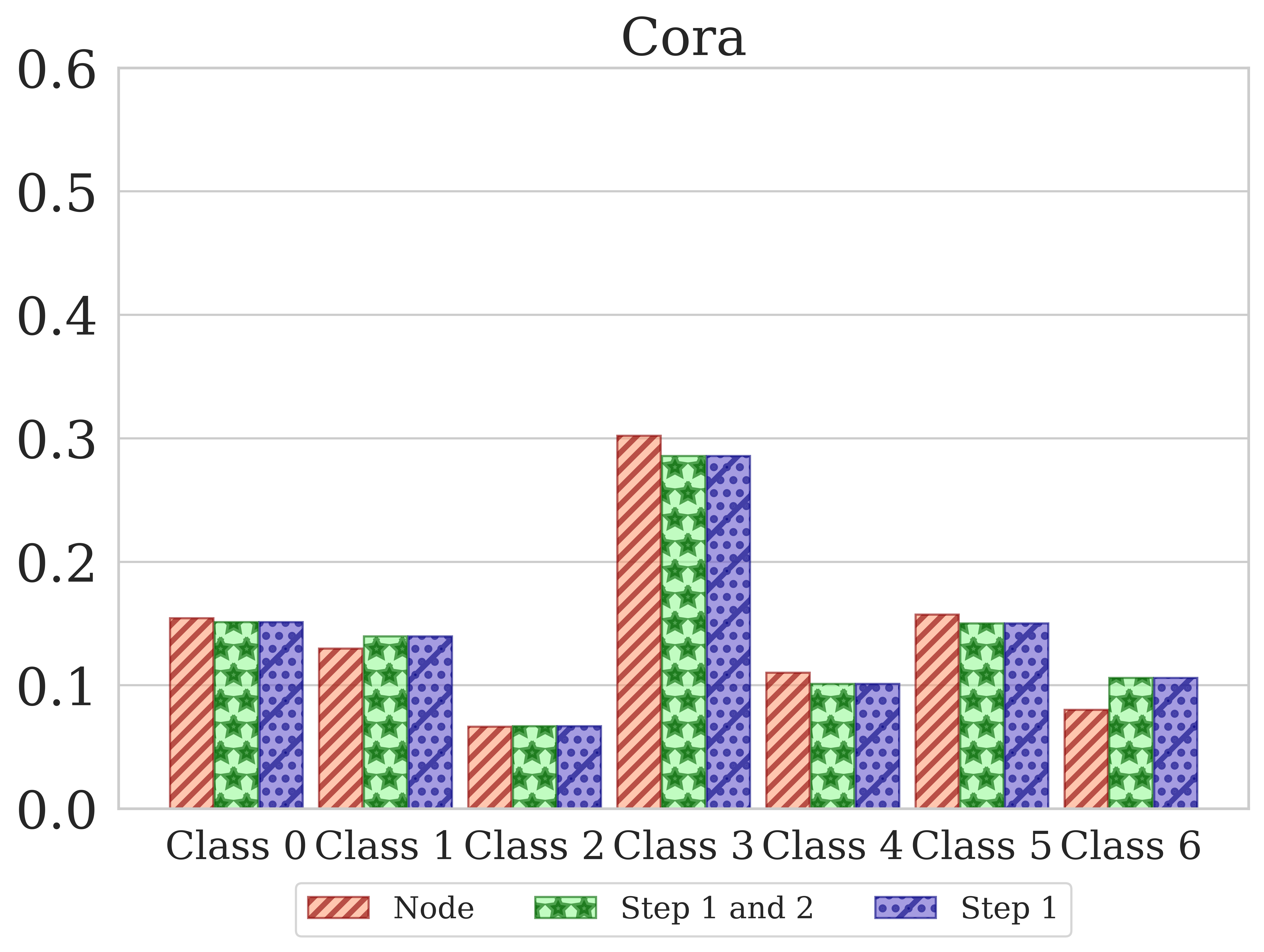
(a) Class distribution for Cora.

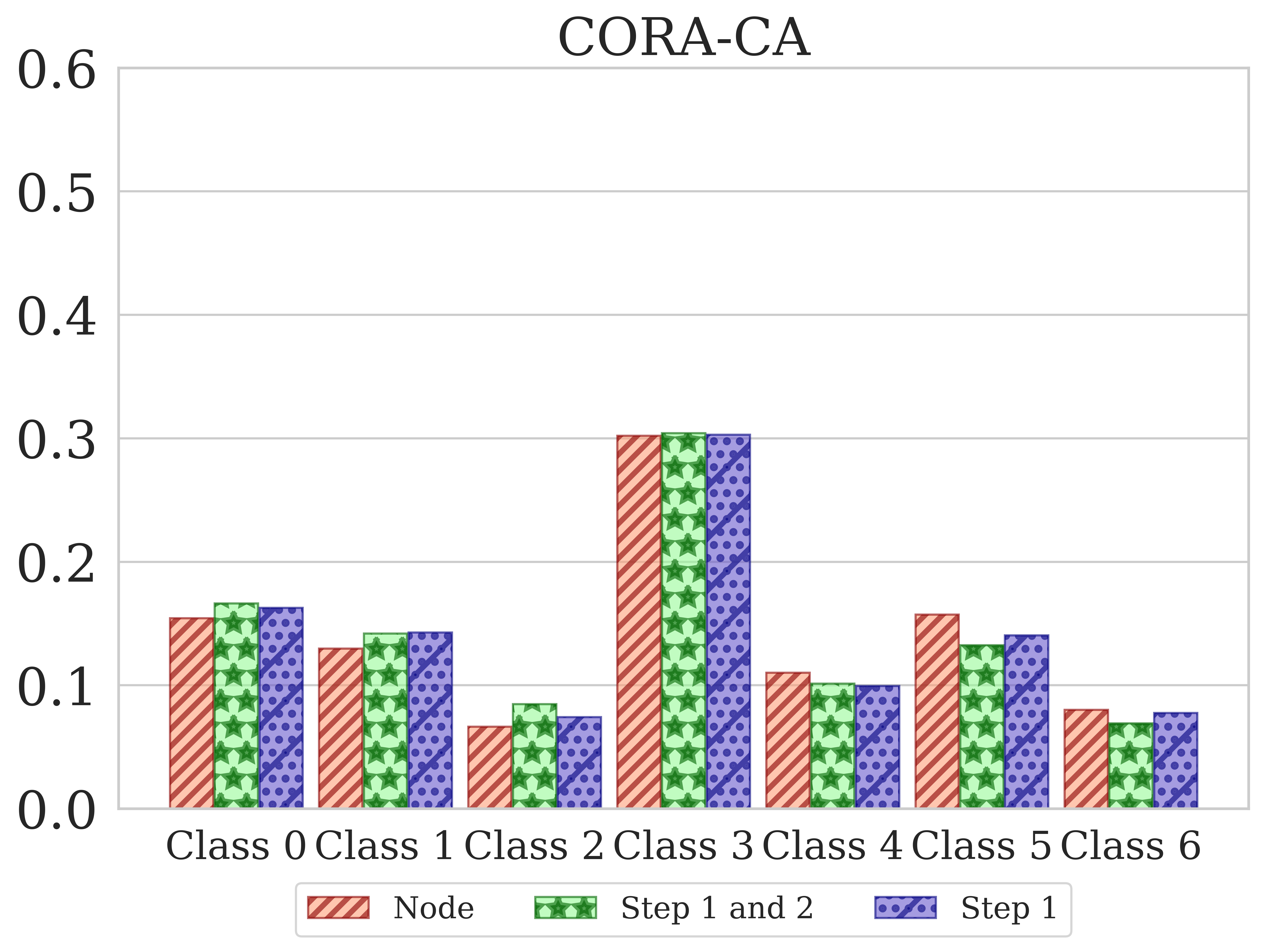
(b) Class distribution for CORA-CA.

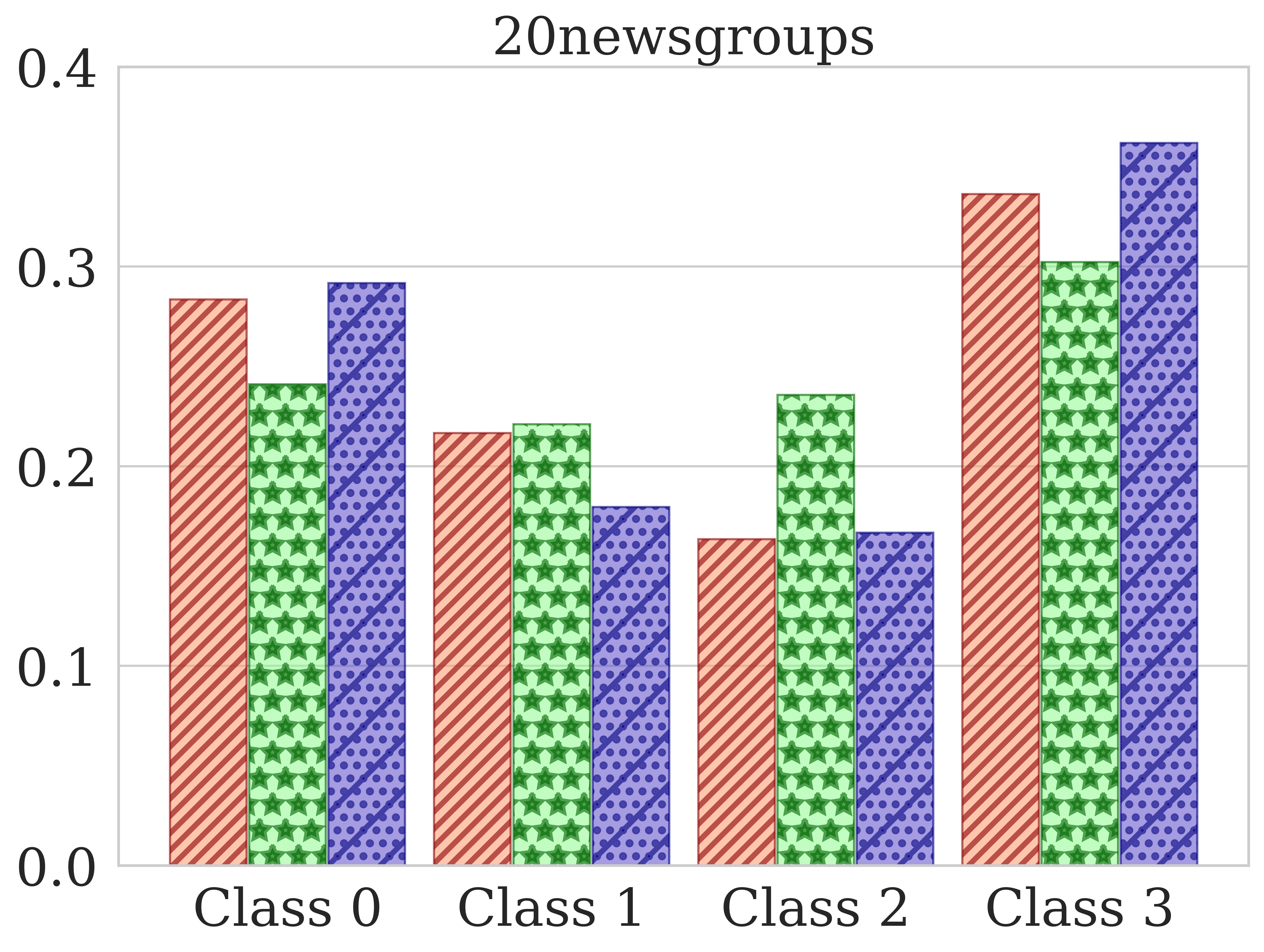
(c) Class distribution for 20Newsgroup.

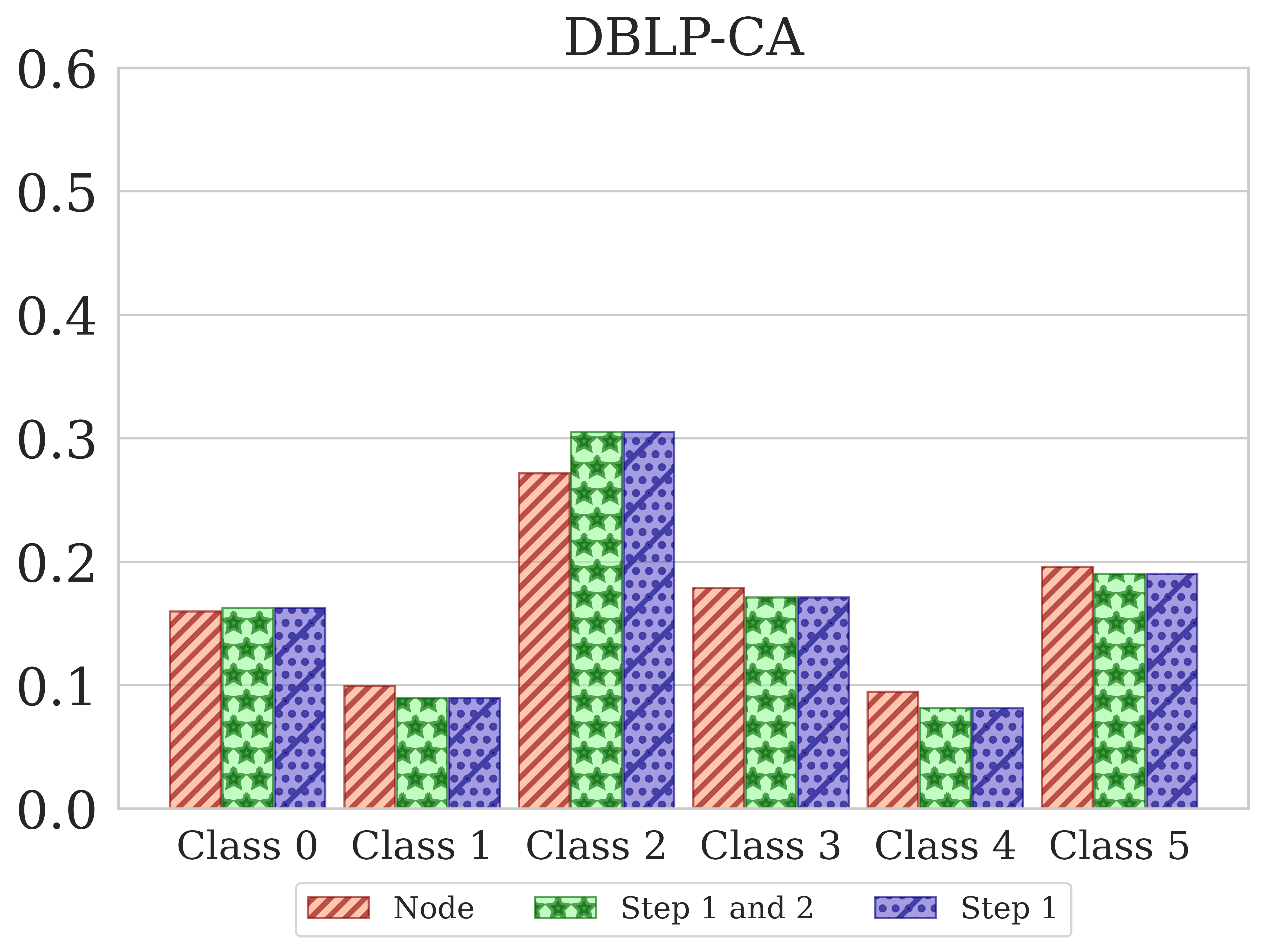
(d) Class distribution for DBLP-CA.

(e) Class distribution for Mushroom.

(f) Class distribution for 20NewsW100.

Figure 16: Class distribution shifts.

References

- Agarwal et al. (2006) Agarwal, S., Branson, K., and Belongie, S. Higher order learning with graphs. In Proceedings of the 23rd international conference on Machine learning, pp. 17–24, 2006.
- Aponte et al. (2022) Aponte, R., Rossi, R. A., Guo, S., Hoffswell, J., Lipka, N., Xiao, C., Chan, G., Koh, E., and Ahmed, N. A hypergraph neural network framework for learning hyperedge-dependent node embeddings. arXiv preprint arXiv:2212.14077, 2022.
- Arya et al. (2020) Arya, D., Gupta, D. K., Rudinac, S., and Worring, M. Hypersage: Generalizing inductive representation learning on hypergraphs. arXiv preprint arXiv:2010.04558, 2020.
- Ba et al. (2016) Ba, J. L., Kiros, J. R., and Hinton, G. E. Layer normalization. arXiv preprint arXiv:1607.06450, 2016.
- Bai et al. (2021) Bai, S., Zhang, F., and Torr, P. H. Hypergraph convolution and hypergraph attention. Pattern Recognition, 110:107637, 2021.
- Balcilar et al. (2021) Balcilar, M., Héroux, P., Gauzere, B., Vasseur, P., Adam, S., and Honeine, P. Breaking the limits of message passing graph neural networks. In International Conference on Machine Learning, pp. 599–608. PMLR, 2021.
- Chen et al. (2003) Chen, D.-Y., Tian, X.-P., Shen, Y.-T., and Ouhyoung, M. On visual similarity based 3d model retrieval. In Computer graphics forum, volume 22, pp. 223–232. Wiley Online Library, 2003.
- Chen & Zhang (2022) Chen, G. and Zhang, J. Preventing over-smoothing for hypergraph neural networks. arXiv preprint arXiv:2203.17159, 2022.
- Chen et al. (2020) Chen, M., Wei, Z., Huang, Z., Ding, B., and Li, Y. Simple and deep graph convolutional networks. In International conference on machine learning, pp. 1725–1735. PMLR, 2020.
- Chien et al. (2020) Chien, E., Peng, J., Li, P., and Milenkovic, O. Adaptive universal generalized pagerank graph neural network. arXiv preprint arXiv:2006.07988, 2020.
- Chien et al. (2022) Chien, E., Pan, C., Peng, J., and Milenkovic, O. You are allset: A multiset function framework for hypergraph neural networks. In International Conference on Learning Representations, 2022. URL https://openreview.net/forum?id=hpBTIv2uy_E.
- Choe et al. (2023) Choe, M., Kim, S., Yoo, J., and Shin, K. Classification of edge-dependent labels of nodes in hypergraphs. arXiv preprint arXiv:2306.03032, 2023.
- Dong et al. (2020) Dong, Y., Sawin, W., and Bengio, Y. Hnhn: Hypergraph networks with hyperedge neurons. arXiv preprint arXiv:2006.12278, 2020.
- Dua et al. (2017) Dua, D., Graff, C., et al. Uci machine learning repository, 2017. URL http://archive. ics. uci. edu/ml, 7(1), 2017.
- Feng et al. (2019) Feng, Y., You, H., Zhang, Z., Ji, R., and Gao, Y. Hypergraph neural networks. In Proceedings of the AAAI conference on artificial intelligence, volume 33, pp. 3558–3565, 2019.
- Gu et al. (2020) Gu, F., Chang, H., Zhu, W., Sojoudi, S., and El Ghaoui, L. Implicit graph neural networks. Advances in Neural Information Processing Systems, 33:11984–11995, 2020.
- Halcrow et al. (2020) Halcrow, J., Mosoi, A., Ruth, S., and Perozzi, B. Grale: Designing networks for graph learning. In Proceedings of the 26th ACM SIGKDD international conference on knowledge discovery & data mining, pp. 2523–2532, 2020.
- Han et al. (2023) Han, Y., Huang, E. W., Zheng, W., Rao, N., Wang, Z., and Subbian, K. Search behavior prediction: A hypergraph perspective. In Proceedings of the Sixteenth ACM International Conference on Web Search and Data Mining, pp. 697–705, 2023.
- Hein et al. (2013) Hein, M., Setzer, S., Jost, L., and Rangapuram, S. S. The total variation on hypergraphs-learning on hypergraphs revisited. Advances in Neural Information Processing Systems, 26, 2013.
- Huang & Yang (2021) Huang, J. and Yang, J. Unignn: a unified framework for graph and hypergraph neural networks. In Zhou, Z.-H. (ed.), Proceedings of the Thirtieth International Joint Conference on Artificial Intelligence, IJCAI-21, pp. 2563–2569. International Joint Conferences on Artificial Intelligence Organization, 8 2021. doi: 10.24963/ijcai.2021/353. URL https://doi.org/10.24963/ijcai.2021/353. Main Track.
- Kipf & Welling (2017) Kipf, T. N. and Welling, M. Semi-supervised classification with graph convolutional networks. In International Conference on Learning Representations, 2017.
- La Gatta et al. (2022) La Gatta, V., Moscato, V., Pennone, M., Postiglione, M., and Sperlí, G. Music recommendation via hypergraph embedding. IEEE Transactions on Neural Networks and Learning Systems, 2022.
- Lee et al. (2019) Lee, J., Lee, Y., Kim, J., Kosiorek, A., Choi, S., and Teh, Y. W. Set transformer: A framework for attention-based permutation-invariant neural networks. In International conference on machine learning, pp. 3744–3753. PMLR, 2019.
- Li et al. (2022) Li, J., Hua, C., Park, J., Ma, H., Dax, V., and Kochenderfer, M. J. Evolvehypergraph: Group-aware dynamic relational reasoning for trajectory prediction. arXiv preprint arXiv:2208.05470, 2022.
- Li & Milenkovic (2017) Li, P. and Milenkovic, O. Inhomogeneous hypergraph clustering with applications. Advances in neural information processing systems, 30, 2017.
- Pei et al. (2020) Pei, H., Wei, B., Chang, K. C.-C., Lei, Y., and Yang, B. Geom-gcn: Geometric graph convolutional networks. arXiv preprint arXiv:2002.05287, 2020.
- Su et al. (2015) Su, H., Maji, S., Kalogerakis, E., and Learned-Miller, E. Multi-view convolutional neural networks for 3d shape recognition. In Proceedings of the IEEE international conference on computer vision, pp. 945–953, 2015.
- Sun et al. (2023) Sun, X., Cheng, H., Liu, B., Li, J., Chen, H., Xu, G., and Yin, H. Self-supervised hypergraph representation learning for sociological analysis. IEEE Transactions on Knowledge and Data Engineering, 2023.
- Teney et al. (2023) Teney, D., Wang, J., and Abbasnejad, E. Selective mixup helps with distribution shifts, but not (only) because of mixup. arXiv preprint arXiv:2305.16817, 2023.
- Tolstikhin et al. (2021) Tolstikhin, I. O., Houlsby, N., Kolesnikov, A., Beyer, L., Zhai, X., Unterthiner, T., Yung, J., Steiner, A., Keysers, D., Uszkoreit, J., et al. Mlp-mixer: An all-mlp architecture for vision. Advances in neural information processing systems, 34:24261–24272, 2021.
- Vaswani et al. (2017) Vaswani, A., Shazeer, N., Parmar, N., Uszkoreit, J., Jones, L., Gomez, A. N., Kaiser, Ł., and Polosukhin, I. Attention is all you need. Advances in neural information processing systems, 30, 2017.
- Veldt et al. (2023) Veldt, N., Benson, A. R., and Kleinberg, J. Combinatorial characterizations and impossibilities for higher-order homophily. Science Advances, 9(1):eabq3200, 2023.
- Veličković et al. (2017) Veličković, P., Cucurull, G., Casanova, A., Romero, A., Lio, P., and Bengio, Y. Graph attention networks. arXiv preprint arXiv:1710.10903, 2017.
- Wang et al. (2023) Wang, P., Yang, S., Liu, Y., Wang, Z., and Li, P. Equivariant hypergraph diffusion neural operators. In The Eleventh International Conference on Learning Representations, 2023. URL https://openreview.net/forum?id=RiTjKoscnNd.
- Wang et al. (2019) Wang, X., Ji, H., Shi, C., Wang, B., Ye, Y., Cui, P., and Yu, P. S. Heterogeneous graph attention network. In The world wide web conference, pp. 2022–2032, 2019.
- Wei et al. (2021) Wei, J., Wang, Y., Guo, M., Lv, P., Yang, X., and Xu, M. Dynamic hypergraph convolutional networks for skeleton-based action recognition. arXiv preprint arXiv:2112.10570, 2021.
- Wu et al. (2015) Wu, Z., Song, S., Khosla, A., Yu, F., Zhang, L., Tang, X., and Xiao, J. 3d shapenets: A deep representation for volumetric shapes. In Proceedings of the IEEE conference on computer vision and pattern recognition, pp. 1912–1920, 2015.
- Xu et al. (2022) Xu, C., Li, M., Ni, Z., Zhang, Y., and Chen, S. Groupnet: Multiscale hypergraph neural networks for trajectory prediction with relational reasoning. In Proceedings of the IEEE/CVF Conference on Computer Vision and Pattern Recognition, pp. 6498–6507, 2022.
- Yadati et al. (2019) Yadati, N., Nimishakavi, M., Yadav, P., Nitin, V., Louis, A., and Talukdar, P. Hypergcn: A new method for training graph convolutional networks on hypergraphs. Advances in neural information processing systems, 32, 2019.
- Yadati et al. (2020) Yadati, N., Nitin, V., Nimishakavi, M., Yadav, P., Louis, A., and Talukdar, P. Nhp: Neural hypergraph link prediction. In Proceedings of the 29th ACM International Conference on Information & Knowledge Management, CIKM ’20, pp. 1705–1714, New York, NY, USA, 2020. Association for Computing Machinery. ISBN 9781450368599. doi: 10.1145/3340531.3411870. URL https://doi.org/10.1145/3340531.3411870.
- Yang et al. (2020) Yang, C., Wang, R., Yao, S., and Abdelzaher, T. Hypergraph learning with line expansion. arXiv preprint arXiv:2005.04843, 2020.
- Yi & Park (2020) Yi, J. and Park, J. Hypergraph convolutional recurrent neural network. In Proceedings of the 26th ACM SIGKDD international conference on knowledge discovery & data mining, pp. 3366–3376, 2020.
- Yu et al. (2021) Yu, J., Yin, H., Li, J., Wang, Q., Hung, N. Q. V., and Zhang, X. Self-supervised multi-channel hypergraph convolutional network for social recommendation. In Proceedings of the web conference 2021, pp. 413–424, 2021.
- Zaheer et al. (2017) Zaheer, M., Kottur, S., Ravanbakhsh, S., Poczos, B., Salakhutdinov, R. R., and Smola, A. J. Deep sets. Advances in neural information processing systems, 30, 2017.
- Zhang et al. (2018) Zhang, M., Cui, Z., Jiang, S., and Chen, Y. Beyond link prediction: Predicting hyperlinks in adjacency space. In Proceedings of the AAAI Conference on Artificial Intelligence, volume 32, 2018.
- Zhou et al. (2006) Zhou, D., Huang, J., and Schölkopf, B. Learning with hypergraphs: Clustering, classification, and embedding. Advances in neural information processing systems, 19, 2006.
- Zhou et al. (2020) Zhou, J., Cui, G., Hu, S., Zhang, Z., Yang, C., Liu, Z., Wang, L., Li, C., and Sun, M. Graph neural networks: A review of methods and applications. AI open, 1:57–81, 2020.