2 Construction of an exact selector
For each u ∈ 𝒰 k , d 𝑢 subscript 𝒰 𝑘 𝑑
u\in{\cal U}_{k,d} r ε , k > 0 subscript 𝑟 𝜀 𝑘
0 r_{\varepsilon,k}>0
a ε , u 2 ( r ε , k ) = 1 2 ε 4 inf 𝜽 ∈ Θ ̊ 𝐜 , u ( r ε , k ) ∑ ℓ ∈ ℤ ̊ u θ ℓ 4 , subscript superscript 𝑎 2 𝜀 𝑢
subscript 𝑟 𝜀 𝑘
1 2 superscript 𝜀 4 subscript infimum 𝜽 subscript ̊ Θ 𝐜 𝑢
subscript 𝑟 𝜀 𝑘
subscript bold-ℓ subscript ̊ ℤ 𝑢 subscript superscript 𝜃 4 bold-ℓ a^{2}_{\varepsilon,u}(r_{\varepsilon,k})=\frac{1}{2\varepsilon^{4}}\inf_{{\boldsymbol{\theta}}\in\mathring{\Theta}_{{\bf c},u}(r_{\varepsilon,k})}\sum_{{\boldsymbol{\ell}}\in\mathring{\mathbb{Z}}_{u}}\theta^{4}_{\boldsymbol{\ell}}, (18)
which plays a key role in the minimax theory of hypothesis testing.
In particular, the problem of testing H 0 , u ′ : 𝜽 u = 𝟎 : subscript superscript 𝐻 ′ 0 𝑢
subscript 𝜽 𝑢 0 H^{\prime}_{0,u}:{\boldsymbol{\theta}}_{u}=\boldsymbol{0} H 1 , u ′ : 𝜽 u ∈ Θ ̊ 𝐜 , u ( r ε , k ) : subscript superscript 𝐻 ′ 1 𝑢
subscript 𝜽 𝑢 subscript ̊ Θ 𝐜 𝑢
subscript 𝑟 𝜀 𝑘
H^{\prime}_{1,u}:{\boldsymbol{\theta}}_{u}\in\mathring{\Theta}_{{\bf c},u}(r_{\varepsilon,k}) r ε , k / r ε , k ∗ → ∞ → subscript 𝑟 𝜀 𝑘
subscript superscript 𝑟 𝜀 𝑘
r_{\varepsilon,k}/r^{*}_{\varepsilon,k}\to\infty separation rate r ε , k ∗ subscript superscript 𝑟 𝜀 𝑘
r^{*}_{\varepsilon,k} a ε , u ( r ε , k ∗ ) ≍ 1 asymptotically-equals subscript 𝑎 𝜀 𝑢
subscript superscript 𝑟 𝜀 𝑘
1 a_{\varepsilon,u}(r^{*}_{\varepsilon,k})\asymp 1 a ε , u ( r ε , k ) subscript 𝑎 𝜀 𝑢
subscript 𝑟 𝜀 𝑘
a_{\varepsilon,u}(r_{\varepsilon,k}) γ > 0 𝛾 0 \gamma>0 ε ∗ > 0 superscript 𝜀 0 \varepsilon^{*}>0 δ ∗ > 0 superscript 𝛿 0 \delta^{*}>0 [12 ] )
a ε , u ( r ε , k ) ≤ a ε , u ( ( 1 + δ ) r ε , k ) ≤ ( 1 + γ ) a ε , u ( r ε , k ) , ∀ ε ∈ ( 0 , ε ∗ ) , ∀ δ ∈ ( 0 , δ ∗ ) . formulae-sequence subscript 𝑎 𝜀 𝑢
subscript 𝑟 𝜀 𝑘
subscript 𝑎 𝜀 𝑢
1 𝛿 subscript 𝑟 𝜀 𝑘
1 𝛾 subscript 𝑎 𝜀 𝑢
subscript 𝑟 𝜀 𝑘
formulae-sequence for-all 𝜀 0 superscript 𝜀 for-all 𝛿 0 superscript 𝛿 a_{\varepsilon,u}(r_{\varepsilon,k})\leq a_{\varepsilon,u}((1+\delta)r_{\varepsilon,k})\leq(1+\gamma)a_{\varepsilon,u}(r_{\varepsilon,k}),\quad\forall\,\varepsilon\in(0,\varepsilon^{*}),\forall\,\delta\in(0,\delta^{*}). (19)
These and other general facts of the minimax hypothesis testing theory can be found in
a series of review articles [7 ] –[9 ] and monograph [12 ] .
Denote the minimizing sequence in (18 ( θ ℓ ∗ ( r ε , k ) ) ℓ ∈ ℤ ̊ u subscript subscript superscript 𝜃 bold-ℓ subscript 𝑟 𝜀 𝑘
bold-ℓ subscript ̊ ℤ 𝑢 (\theta^{*}_{\boldsymbol{\ell}}(r_{\varepsilon,k}))_{{\boldsymbol{\ell}}\in\mathring{\mathbb{Z}}_{u}}
a ε , u 2 ( r ε , k ) = 1 2 ε 4 ∑ ℓ ∈ ℤ ̊ u [ θ ℓ ∗ ( r ε , k ) ] 4 subscript superscript 𝑎 2 𝜀 𝑢
subscript 𝑟 𝜀 𝑘
1 2 superscript 𝜀 4 subscript bold-ℓ subscript ̊ ℤ 𝑢 superscript delimited-[] subscript superscript 𝜃 bold-ℓ subscript 𝑟 𝜀 𝑘
4 a^{2}_{\varepsilon,u}(r_{\varepsilon,k})=\frac{1}{2\varepsilon^{4}}\sum_{{\boldsymbol{\ell}}\in\mathring{\mathbb{Z}}_{u}}\left[\theta^{*}_{\boldsymbol{\ell}}(r_{\varepsilon,k})\right]^{4} (20)
and let r ε , k ∗ > 0 subscript superscript 𝑟 𝜀 𝑘
0 r^{*}_{\varepsilon,k}>0 [10 ] ,
a ε , u ( r ε , k ∗ ) = ( 1 + 1 − β ) 2 log ( d k ) . subscript 𝑎 𝜀 𝑢
subscript superscript 𝑟 𝜀 𝑘
1 1 𝛽 2 binomial 𝑑 𝑘 a_{\varepsilon,u}(r^{*}_{\varepsilon,k})=(1+\sqrt{1-\beta})\sqrt{2\log{d\choose k}}. (21)
For the purpose of constructing an exact selector 𝜼 ^ ^ 𝜼 \hat{{\boldsymbol{\eta}}} 15 χ 2 superscript 𝜒 2 \chi^{2} [10 ] ,
S u = ∑ ℓ ∈ ℤ ̊ u ω ℓ ( r ε , k ∗ ) [ ( X ℓ / ε ) 2 − 1 ] , u ∈ 𝒰 k , d , formulae-sequence subscript 𝑆 𝑢 subscript bold-ℓ subscript ̊ ℤ 𝑢 subscript 𝜔 bold-ℓ subscript superscript 𝑟 𝜀 𝑘
delimited-[] superscript subscript 𝑋 bold-ℓ 𝜀 2 1 𝑢 subscript 𝒰 𝑘 𝑑
S_{u}=\sum_{{\boldsymbol{\ell}}\in\mathring{\mathbb{Z}}_{u}}\omega_{\boldsymbol{\ell}}(r^{*}_{\varepsilon,k})\left[\left({X_{\boldsymbol{\ell}}}/{\varepsilon}\right)^{2}-1\right],\quad u\in{\cal U}_{k,d}, (22)
where
ω ℓ ( r ε , k ) = 1 2 ε 2 [ θ ℓ ∗ ( r ε , k ) ] 2 a ε , u ( r ε , k ) , ℓ ∈ ℤ ̊ u . formulae-sequence subscript 𝜔 bold-ℓ subscript 𝑟 𝜀 𝑘
1 2 superscript 𝜀 2 superscript delimited-[] subscript superscript 𝜃 bold-ℓ subscript 𝑟 𝜀 𝑘
2 subscript 𝑎 𝜀 𝑢
subscript 𝑟 𝜀 𝑘
bold-ℓ subscript ̊ ℤ 𝑢 \omega_{\boldsymbol{\ell}}(r_{\varepsilon,k})=\frac{1}{2\varepsilon^{2}}\frac{[\theta^{*}_{\boldsymbol{\ell}}(r_{\varepsilon,k})]^{2}}{a_{\varepsilon,u}(r_{\varepsilon,k})},\quad{\boldsymbol{\ell}}\in\mathring{\mathbb{Z}}_{u}. (23)
Due to (20
∑ ℓ ∈ ℤ ̊ u ω ℓ 2 ( r ε , k ) = 1 / 2 for all r ε , k > 0 . formulae-sequence subscript bold-ℓ subscript ̊ ℤ 𝑢 superscript subscript 𝜔 bold-ℓ 2 subscript 𝑟 𝜀 𝑘
1 2 for all subscript 𝑟 𝜀 𝑘
0 \sum_{{\boldsymbol{\ell}}\in\mathring{\mathbb{Z}}_{u}}\omega_{\boldsymbol{\ell}}^{2}(r_{\varepsilon,k})={1}/{2}\quad\mbox{for all}\;\;r_{\varepsilon,k}>0. (24)
It is known (see, for example, Remark 2.1 of [13 ] or Theorem 4 of [11 ] ) that
[ θ ℓ ∗ ( r ε , k ) ] 2 = a 0 2 ( 1 − ( c ℓ / T ) 2 ) + , superscript delimited-[] subscript superscript 𝜃 bold-ℓ subscript 𝑟 𝜀 𝑘
2 superscript subscript 𝑎 0 2 subscript 1 superscript subscript 𝑐 bold-ℓ 𝑇 2 [\theta^{*}_{\boldsymbol{\ell}}(r_{\varepsilon,k})]^{2}=a_{0}^{2}\left(1-(c_{{\boldsymbol{\ell}}}/T)^{2}\right)_{+}, (25)
where the collection ( c ℓ ) ℓ ∈ ℤ ̊ u subscript subscript 𝑐 bold-ℓ bold-ℓ subscript ̊ ℤ 𝑢 (c_{\boldsymbol{\ell}})_{{{\boldsymbol{\ell}}\in\mathring{\mathbb{Z}}_{u}}} 8 a 0 2 = a 0 , ε , k 2 superscript subscript 𝑎 0 2 superscript subscript 𝑎 0 𝜀 𝑘
2 a_{0}^{2}=a_{0,\varepsilon,k}^{2} T = T ε , k 𝑇 subscript 𝑇 𝜀 𝑘
T=T_{\varepsilon,k}
a 0 2 ∑ ℓ ∈ ℤ ̊ u ( 1 − ( c ℓ / T ) 2 ) = r ε , k 2 , a 0 2 ∑ ℓ ∈ ℤ ̊ u c ℓ 2 ( 1 − ( c ℓ / T ) 2 ) = 1 , T ≥ r ε , k − 1 → ∞ . formulae-sequence superscript subscript 𝑎 0 2 subscript bold-ℓ subscript ̊ ℤ 𝑢 1 superscript subscript 𝑐 bold-ℓ 𝑇 2 superscript subscript 𝑟 𝜀 𝑘
2 formulae-sequence superscript subscript 𝑎 0 2 subscript bold-ℓ subscript ̊ ℤ 𝑢 superscript subscript 𝑐 bold-ℓ 2 1 superscript subscript 𝑐 bold-ℓ 𝑇 2 1 𝑇 subscript superscript 𝑟 1 𝜀 𝑘
→ \displaystyle a_{0}^{2}\sum_{{\boldsymbol{\ell}}\in\mathring{\mathbb{Z}}_{u}}\left(1-(c_{{\boldsymbol{\ell}}}/T)^{2}\right)=r_{\varepsilon,k}^{2},\quad a_{0}^{2}\sum_{{\boldsymbol{\ell}}\in\mathring{\mathbb{Z}}_{u}}c_{{\boldsymbol{\ell}}}^{2}\left(1-(c_{{\boldsymbol{\ell}}}/T)^{2}\right)=1,\quad T\geq r^{-1}_{\varepsilon,k}\to\infty.
For fixed k 𝑘 k [11 ] and its proof,
we can easily get the asymptotic expressions for a 0 2 superscript subscript 𝑎 0 2 a_{0}^{2} T 𝑇 T 25 ℓ ∈ ℤ ̊ u bold-ℓ subscript ̊ ℤ 𝑢 {\boldsymbol{\ell}}\in\mathring{\mathbb{Z}}_{u} 8 ε → 0 → 𝜀 0 \varepsilon\to 0
[ θ ℓ ∗ ( r ε , k ) ] 2 ∼ r ε , k 2 + k / σ 2 k π k / 2 ( k + 2 σ ) Γ ( 1 + k / 2 ) 2 σ ( 1 + 4 σ / k ) k / ( 2 σ ) ( 1 − ( ∑ j = 1 d ( 2 π l j ) 2 ) σ r ε , k 2 ( 1 + 4 σ / k ) ) + . similar-to superscript delimited-[] subscript superscript 𝜃 bold-ℓ subscript 𝑟 𝜀 𝑘
2 superscript subscript 𝑟 𝜀 𝑘
2 𝑘 𝜎 superscript 2 𝑘 superscript 𝜋 𝑘 2 𝑘 2 𝜎 Γ 1 𝑘 2 2 𝜎 superscript 1 4 𝜎 𝑘 𝑘 2 𝜎 subscript 1 superscript superscript subscript 𝑗 1 𝑑 superscript 2 𝜋 subscript 𝑙 𝑗 2 𝜎 subscript superscript 𝑟 2 𝜀 𝑘
1 4 𝜎 𝑘 \displaystyle[\theta^{*}_{\boldsymbol{\ell}}(r_{\varepsilon,k})]^{2}\sim\frac{r_{\varepsilon,k}^{2+{k}/{\sigma}}2^{k}\pi^{{k}/{2}}(k+2\sigma)\Gamma\left(1+{k}/{2}\right)}{2\sigma\left(1+4\sigma/k\right)^{{k}/{(2\sigma)}}}\left(1-\left(\sum\nolimits_{j=1}^{d}(2\pi l_{j})^{2}\right)^{\sigma}\frac{r^{2}_{\varepsilon,k}}{(1+4\sigma/k)}\right)_{+}. (26)
Since
# { ℓ ∈ ℤ ̊ u : θ ℓ ∗ ( r ε , k ) ≠ 0 } = # { ℓ ∈ ℤ ̊ u : ( ∑ j = 1 d l j 2 ) 1 / 2 < ( 1 + 4 σ / k ) 1 / ( 2 σ ) / ( 2 π r ε , k 1 / σ ) } # conditional-set bold-ℓ subscript ̊ ℤ 𝑢 subscript superscript 𝜃 bold-ℓ subscript 𝑟 𝜀 𝑘
0 # conditional-set bold-ℓ subscript ̊ ℤ 𝑢 superscript superscript subscript 𝑗 1 𝑑 superscript subscript 𝑙 𝑗 2 1 2 superscript 1 4 𝜎 𝑘 1 2 𝜎 2 𝜋 superscript subscript 𝑟 𝜀 𝑘
1 𝜎 \#\{{\boldsymbol{\ell}}\in\mathring{\mathbb{Z}}_{u}:\theta^{*}_{\boldsymbol{\ell}}(r_{\varepsilon,k})\neq 0\}=\#\left\{{\boldsymbol{\ell}}\in\mathring{\mathbb{Z}}_{u}:\left(\sum_{j=1}^{d}l_{j}^{2}\right)^{1/2}<(1+4\sigma/k)^{1/(2\sigma)}/(2\pi r_{\varepsilon,k}^{1/\sigma})\right\} l 2 subscript 𝑙 2 l_{2} ( 1 + 4 σ / k ) 1 / ( 2 σ ) / ( 2 π r ε , k 1 / σ ) superscript 1 4 𝜎 𝑘 1 2 𝜎 2 𝜋 superscript subscript 𝑟 𝜀 𝑘
1 𝜎 (1+4\sigma/k)^{1/(2\sigma)}/(2\pi r_{\varepsilon,k}^{1/\sigma}) ℝ k superscript ℝ 𝑘 \mathbb{R}^{k} 𝒪 ( r ε , k − k / σ ) 𝒪 superscript subscript 𝑟 𝜀 𝑘
𝑘 𝜎 \mathcal{O}(r_{\varepsilon,k}^{-{k}/{\sigma}})
# { ℓ ∈ ℤ ̊ u : θ ℓ ∗ ( r ε , k ) ≠ 0 } ≍ r ε , k − k / σ , ε → 0 , formulae-sequence asymptotically-equals # conditional-set bold-ℓ subscript ̊ ℤ 𝑢 subscript superscript 𝜃 bold-ℓ subscript 𝑟 𝜀 𝑘
0 superscript subscript 𝑟 𝜀 𝑘
𝑘 𝜎 → 𝜀 0 \displaystyle\#\{{\boldsymbol{\ell}}\in\mathring{\mathbb{Z}}_{u}:\theta^{*}_{\boldsymbol{\ell}}(r_{\varepsilon,k})\neq 0\}\asymp r_{\varepsilon,k}^{-{k}/{\sigma}},\quad\varepsilon\to 0,
when both k 𝑘 k k = k ε → ∞ 𝑘 subscript 𝑘 𝜀 → k=k_{\varepsilon}\to\infty
We can modify the asymptotic expression in (26 k = k ε → ∞ 𝑘 subscript 𝑘 𝜀 → k=k_{\varepsilon}\to\infty Γ ( x + 1 ) ∼ 2 π x x + 1 / 2 e − x similar-to Γ 𝑥 1 2 𝜋 superscript 𝑥 𝑥 1 2 superscript 𝑒 𝑥 \Gamma(x+1)\sim\sqrt{2\pi}x^{x+1/2}e^{-x} ( 1 + 1 / x ) x ∼ e similar-to superscript 1 1 𝑥 𝑥 𝑒 (1+1/x)^{x}\sim e x → ∞ → 𝑥 x\to\infty
[ θ ℓ ∗ ( r ε , k ) ] 2 ∼ r ε , k 2 + k / σ π 1 / 2 ( 2 π k / e ) k / 2 k 3 / 2 2 σ e 2 ( 1 − ( ∑ j = 1 d ( 2 π l j ) 2 ) σ r ε , k 2 ( 1 + 4 σ / k ) ) + , ε → 0 . formulae-sequence similar-to superscript delimited-[] subscript superscript 𝜃 bold-ℓ subscript 𝑟 𝜀 𝑘
2 superscript subscript 𝑟 𝜀 𝑘
2 𝑘 𝜎 superscript 𝜋 1 2 superscript 2 𝜋 𝑘 𝑒 𝑘 2 superscript 𝑘 3 2 2 𝜎 superscript 𝑒 2 subscript 1 superscript superscript subscript 𝑗 1 𝑑 superscript 2 𝜋 subscript 𝑙 𝑗 2 𝜎 subscript superscript 𝑟 2 𝜀 𝑘
1 4 𝜎 𝑘 → 𝜀 0 \displaystyle[\theta^{*}_{\boldsymbol{\ell}}(r_{\varepsilon,k})]^{2}\sim\frac{r_{\varepsilon,k}^{2+{k}/{\sigma}}\pi^{1/2}(2\pi k/e)^{k/2}k^{3/2}}{2\sigma e^{2}}\left(1-\left(\sum\nolimits_{j=1}^{d}(2\pi l_{j})^{2}\right)^{\sigma}\frac{r^{2}_{\varepsilon,k}}{(1+4\sigma/k)}\right)_{+},\quad\varepsilon\to 0. (27)
In both cases, when k 𝑘 k k = k ε → ∞ 𝑘 subscript 𝑘 𝜀 → k=k_{\varepsilon}\to\infty 22 23 S u subscript 𝑆 𝑢 S_{u} u ∈ 𝒰 k , d 𝑢 subscript 𝒰 𝑘 𝑑
u\in{\cal U}_{k,d} 𝒪 ( r ε , k − k / σ ) 𝒪 superscript subscript 𝑟 𝜀 𝑘
𝑘 𝜎 \mathcal{O}(r_{\varepsilon,k}^{-{k}/{\sigma}})
It is also known that for fixed k 𝑘 k a ε , k ( r ε , k ) subscript 𝑎 𝜀 𝑘
subscript 𝑟 𝜀 𝑘
a_{\varepsilon,k}(r_{\varepsilon,k}) ε → 0 → 𝜀 0 \varepsilon\to 0 [11 ] )
a ε , k ( r ε , k ) ∼ C ( σ , k ) r ε , k 2 + k / ( 2 σ ) ε − 2 , C 2 ( σ , k ) = π k ( 1 + 2 σ / k ) Γ ( 1 + k / 2 ) ( 1 + 4 σ / k ) 1 + k / ( 2 σ ) Γ k ( 3 / 2 ) formulae-sequence similar-to subscript 𝑎 𝜀 𝑘
subscript 𝑟 𝜀 𝑘
𝐶 𝜎 𝑘 superscript subscript 𝑟 𝜀 𝑘
2 𝑘 2 𝜎 superscript 𝜀 2 superscript 𝐶 2 𝜎 𝑘 superscript 𝜋 𝑘 1 2 𝜎 𝑘 Γ 1 𝑘 2 superscript 1 4 𝜎 𝑘 1 𝑘 2 𝜎 superscript Γ 𝑘 3 2 \displaystyle a_{\varepsilon,k}(r_{\varepsilon,k})\sim C(\sigma,k)r_{\varepsilon,k}^{2+{k}/{(2\sigma)}}\varepsilon^{-2},\quad C^{2}(\sigma,k)=\frac{\pi^{k}(1+{2\sigma}/{k})\Gamma(1+k/2)}{(1+4\sigma/k)^{1+{k}/{(2\sigma)}}\Gamma^{k}(3/2)} (28)
and, when k = k ε → ∞ 𝑘 subscript 𝑘 𝜀 → k=k_{\varepsilon}\to\infty [11 ] ,
a ε , k ( r ε , k ) ∼ ( 2 π k / e ) k / 4 e − 1 ( π k ) 1 / 4 r ε , k 2 + k / ( 2 σ ) ε − 2 . similar-to subscript 𝑎 𝜀 𝑘
subscript 𝑟 𝜀 𝑘
superscript 2 𝜋 𝑘 𝑒 𝑘 4 superscript 𝑒 1 superscript 𝜋 𝑘 1 4 superscript subscript 𝑟 𝜀 𝑘
2 𝑘 2 𝜎 superscript 𝜀 2 \displaystyle a_{\varepsilon,k}(r_{\varepsilon,k})\sim\left({2\pi k}/{e}\right)^{{k}/{4}}e^{-1}(\pi k)^{1/4}r_{\varepsilon,k}^{2+{k}/{(2\sigma)}}\varepsilon^{-2}. (29)
In case of known β 𝛽 \beta 𝜼 = ( η u ) u ∈ 𝒰 k , d ∈ ℋ k , β d 𝜼 subscript subscript 𝜂 𝑢 𝑢 subscript 𝒰 𝑘 𝑑
subscript superscript ℋ 𝑑 𝑘 𝛽
{\boldsymbol{\eta}}=(\eta_{u})_{u\in{\cal U}_{k,d}}\in{\cal H}^{d}_{k,\beta} 𝜼 ˇ = ( η ˇ u ) u ∈ 𝒰 k , d bold-ˇ 𝜼 subscript subscript ˇ 𝜂 𝑢 𝑢 subscript 𝒰 𝑘 𝑑
\boldsymbol{\check{\eta}}=(\check{\eta}_{u})_{u\in{\cal U}_{k,d}}
η ˇ u = 𝟙 ( S u > ( 2 + ϵ ) log ( d k ) ) , u ∈ 𝒰 k , d , formulae-sequence subscript ˇ 𝜂 𝑢 1 subscript 𝑆 𝑢 2 italic-ϵ binomial 𝑑 𝑘 𝑢 subscript 𝒰 𝑘 𝑑
\check{\eta}_{u}=\mathds{1}\left({S_{u}>\sqrt{(2+\epsilon)\log{d\choose k}}}\right),\quad u\in{\cal U}_{k,d}, (30)
with some ϵ = ϵ ε → 0 italic-ϵ subscript italic-ϵ 𝜀 → 0 \epsilon=\epsilon_{\varepsilon}\to 0 ε → 0 → 𝜀 0 \varepsilon\to 0 β 𝛽 \beta S u subscript 𝑆 𝑢 S_{u} β 𝛽 \beta [10 ] , for a given k 𝑘 k
β k , m = m ρ k , m = 1 , … , M k , formulae-sequence subscript 𝛽 𝑘 𝑚
𝑚 subscript 𝜌 𝑘 𝑚 1 … subscript 𝑀 𝑘
\displaystyle\beta_{k,m}=m\rho_{k},\quad m=1,\ldots,M_{k},
where ρ k > 0 subscript 𝜌 𝑘 0 \rho_{k}>0 ε 𝜀 \varepsilon M k = ⌊ 1 / ρ k ⌋ subscript 𝑀 𝑘 1 subscript 𝜌 𝑘 M_{k}=\lfloor 1/\rho_{k}\rfloor log M k = 𝒪 ( log ( d k ) ) subscript 𝑀 𝑘 𝒪 binomial 𝑑 𝑘 \log M_{k}={{\scriptscriptstyle\mathcal{O}}}\left(\log{d\choose k}\right) ε → 0 → 𝜀 0 \varepsilon\to 0 m = 1 , … , M k 𝑚 1 … subscript 𝑀 𝑘
m=1,\ldots,M_{k} r ε , k , m ∗ > 0 subscript superscript 𝑟 𝜀 𝑘 𝑚
0 r^{*}_{\varepsilon,k,m}>0
a ε , u ( r ε , k , m ∗ ) = ( 1 + 1 − β k , m ) 2 log ( d k ) subscript 𝑎 𝜀 𝑢
subscript superscript 𝑟 𝜀 𝑘 𝑚
1 1 subscript 𝛽 𝑘 𝑚
2 binomial 𝑑 𝑘 a_{\varepsilon,u}(r^{*}_{\varepsilon,k,m})=(1+\sqrt{1-\beta_{k,m}})\sqrt{2\log{d\choose k}} (31)
and for every u ∈ 𝒰 k , d 𝑢 subscript 𝒰 𝑘 𝑑
u\in{\cal U}_{k,d}
S u , m = ∑ ℓ ∈ ℤ ̊ u ω ℓ ( r ε , k , m ∗ ) [ ( X ℓ / ε ) 2 − 1 ] , m = 1 , … , M k . formulae-sequence subscript 𝑆 𝑢 𝑚
subscript bold-ℓ subscript ̊ ℤ 𝑢 subscript 𝜔 bold-ℓ subscript superscript 𝑟 𝜀 𝑘 𝑚
delimited-[] superscript subscript 𝑋 bold-ℓ 𝜀 2 1 𝑚 1 … subscript 𝑀 𝑘
S_{u,m}=\sum_{{\boldsymbol{\ell}}\in\mathring{\mathbb{Z}}_{u}}\omega_{\boldsymbol{\ell}}(r^{*}_{\varepsilon,k,m})\left[\left({X_{\boldsymbol{\ell}}}/{\varepsilon}\right)^{2}-1\right],\quad m=1,\ldots,M_{k}. (32)
Now, we propose a selector 𝜼 ^ = ( η ^ u ) u ∈ 𝒰 k , d bold-^ 𝜼 subscript subscript ^ 𝜂 𝑢 𝑢 subscript 𝒰 𝑘 𝑑
\boldsymbol{\hat{\eta}}=(\hat{\eta}_{u})_{u\in{\cal U}_{k,d}} 30
η ^ u = max 1 ≤ m ≤ M k η ^ u , m , η ^ u , m = 𝟙 ( S u , m > ( 2 + ϵ ) ( log ( d k ) + log M k ) ) , formulae-sequence subscript ^ 𝜂 𝑢 subscript 1 𝑚 subscript 𝑀 𝑘 subscript ^ 𝜂 𝑢 𝑚
subscript ^ 𝜂 𝑢 𝑚
1 subscript 𝑆 𝑢 𝑚
2 italic-ϵ binomial 𝑑 𝑘 subscript 𝑀 𝑘 \hat{\eta}_{u}=\max_{1\leq m\leq M_{k}}\hat{\eta}_{u,m},\quad\hat{\eta}_{u,m}=\mathds{1}\left({S_{u,m}>\sqrt{(2+\epsilon)\left(\log{d\choose k}+\log M_{k}\right)}}\right), (33)
where ϵ > 0 italic-ϵ 0 \epsilon>0 ε 𝜀 \varepsilon
ϵ → 0 and ϵ log ( d k ) → ∞ , as ε → 0 . formulae-sequence → italic-ϵ 0 and
formulae-sequence → italic-ϵ binomial 𝑑 𝑘 → as 𝜀 0 \displaystyle\epsilon\to 0\quad\mbox{and}\quad\epsilon\log{d\choose k}\to\infty,\quad\mbox{as}\;\;\varepsilon\to 0. (34)
In this work, we shall deal with the cases when d = d ε → ∞ 𝑑 subscript 𝑑 𝜀 → d=d_{\varepsilon}\to\infty k 𝑘 k k = k ε → ∞ 𝑘 subscript 𝑘 𝜀 → k=k_{\varepsilon}\to\infty k = 𝒪 ( d ) 𝑘 𝒪 𝑑 k={{\scriptscriptstyle\mathcal{O}}}(d) ε → ∞ → 𝜀 \varepsilon\to\infty
Let us explain the idea behind the selector 𝜼 ^ = ( η ^ u ) u ∈ 𝒰 k , d ^ 𝜼 subscript subscript ^ 𝜂 𝑢 𝑢 subscript 𝒰 𝑘 𝑑
\hat{{\boldsymbol{\eta}}}=(\hat{\eta}_{u})_{u\in{\cal U}_{k,d}} 33 u ∈ 𝒰 k , d 𝑢 subscript 𝒰 𝑘 𝑑
u\in{\cal U}_{k,d} η ^ u subscript ^ 𝜂 𝑢 \hat{\eta}_{u} f u subscript 𝑓 𝑢 f_{u} S u , m subscript 𝑆 𝑢 𝑚
S_{u,m} m = 1 , … , M k 𝑚 1 … subscript 𝑀 𝑘
m=1,\ldots,M_{k} f u subscript 𝑓 𝑢 f_{u} η ^ u subscript ^ 𝜂 𝑢 \hat{\eta}_{u} P η u = 1 ( η ^ u , m 0 = 0 ) subscript 𝑃 subscript 𝜂 𝑢 1 subscript ^ 𝜂 𝑢 subscript 𝑚 0
0 P_{\eta_{u}=1}(\hat{\eta}_{u,m_{0}}=0) β k , m 0 subscript 𝛽 𝑘 subscript 𝑚 0
\beta_{k,m_{0}} β 𝛽 \beta f u subscript 𝑓 𝑢 f_{u} ∑ m = 1 M k P η u = 0 ( η ^ u , m = 1 ) superscript subscript 𝑚 1 subscript 𝑀 𝑘 subscript 𝑃 subscript 𝜂 𝑢 0 subscript ^ 𝜂 𝑢 𝑚
1 \sum_{m=1}^{M_{k}}P_{\eta_{u}=0}(\hat{\eta}_{u,m}=1) 1 𝜼 ^ ^ 𝜼 \hat{{\boldsymbol{\eta}}} σ > 0 𝜎 0 \sigma>0 σ 𝜎 \sigma
4 Simulation study
In this section, we illustrate numerically how the exact selector 𝜼 ^ = ( η ^ u ) u ∈ 𝒰 k , d ^ 𝜼 subscript subscript ^ 𝜂 𝑢 𝑢 subscript 𝒰 𝑘 𝑑
\hat{{\boldsymbol{\eta}}}=(\hat{\eta}_{u})_{u\in{\cal U}_{k,d}} 33 f ∈ ℱ k , σ d ( r ε , k ) 𝑓 superscript subscript ℱ 𝑘 𝜎
𝑑 subscript 𝑟 𝜀 𝑘
f\in{\cal F}_{k,\sigma}^{d}(r_{\varepsilon,k}) f ( 𝐭 ) = ∑ u ∈ 𝒰 k , d η u f u ( 𝐭 u ) 𝑓 𝐭 subscript 𝑢 subscript 𝒰 𝑘 𝑑
subscript 𝜂 𝑢 subscript 𝑓 𝑢 subscript 𝐭 𝑢 f({\bf t})=\sum_{u\in{\cal U}_{k,d}}\eta_{u}f_{u}({\bf t}_{u}) k = 2 𝑘 2 k=2 σ = 1 𝜎 1 \sigma=1 d = 10 , 50 𝑑 10 50
d=10,50 β 𝛽 \beta ( d 2 ) binomial 𝑑 2 {d\choose 2} 𝒰 2 , d subscript 𝒰 2 𝑑
\mathcal{U}_{2,d} d 𝑑 d
The two values of β 𝛽 \beta 3 β = 1 − log ( ∑ u ∈ 𝒰 2 , d η u ) / log ( d k ) 𝛽 1 subscript 𝑢 subscript 𝒰 2 𝑑
subscript 𝜂 𝑢 binomial 𝑑 𝑘 \beta=1-\log\left({\sum\nolimits_{u\in\mathcal{U}_{2,d}}\eta_{u}}\right)/{\log{d\choose k}} 0 < β ≤ 1 / 2 0 𝛽 1 2 0<\beta\leq{1}/{2} 1 / 2 < β < 1 1 2 𝛽 1 {1}/{2}<\beta<1
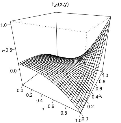
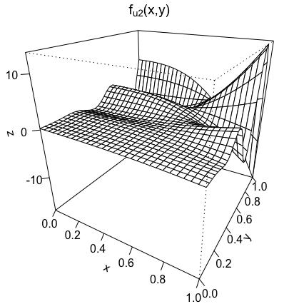
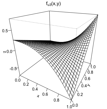
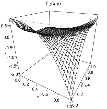
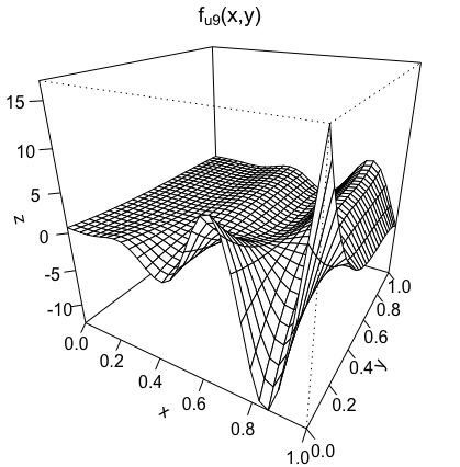
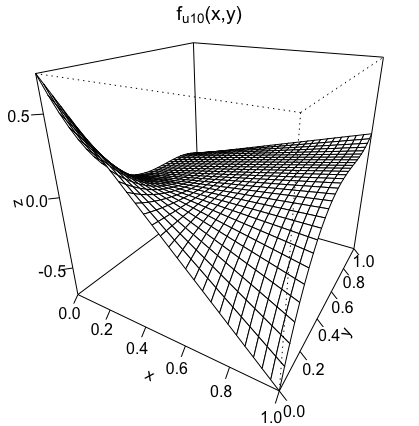
Consider the following five functions defined on [ 0 , 1 ] 0 1 [0,1]
g 1 ( t ) subscript 𝑔 1 𝑡 \displaystyle g_{1}(t) = t 2 ( 2 t − 1 − ( t − 0.5 ) 2 ) exp ( t ) − 0.5424 , absent superscript 𝑡 2 superscript 2 𝑡 1 superscript 𝑡 0.5 2 𝑡 0.5424 \displaystyle=t^{2}(2^{t-1}-(t-0.5)^{2})\exp(t)-0.5424,
g 2 ( t ) subscript 𝑔 2 𝑡 \displaystyle g_{2}(t) = t 2 ( 2 t − 1 − ( t − 1 ) 5 ) − 0.2887 , absent superscript 𝑡 2 superscript 2 𝑡 1 superscript 𝑡 1 5 0.2887 \displaystyle=t^{2}(2^{t-1}-(t-1)^{5})-0.2887,
g 3 ( t ) subscript 𝑔 3 𝑡 \displaystyle g_{3}(t) = 15 t 2 2 t − 1 cos ( 15 t ) − 0.5011 , absent 15 superscript 𝑡 2 superscript 2 𝑡 1 15 𝑡 0.5011 \displaystyle=15t^{2}2^{t-1}\cos(15t)-0.5011,
g 4 ( t ) subscript 𝑔 4 𝑡 \displaystyle g_{4}(t) = t − 1 / 2 , absent 𝑡 1 2 \displaystyle=t-{1}/{2},
g 5 ( t ) subscript 𝑔 5 𝑡 \displaystyle g_{5}(t) = 5 ( t − 0.7 ) 3 + 0.29 , absent 5 superscript 𝑡 0.7 3 0.29 \displaystyle=5(t-0.7)^{3}+0.29,
and let the active components f u subscript 𝑓 𝑢 f_{u} f 𝑓 f [ 0 , 1 ] 2 superscript 0 1 2 [0,1]^{2}
f u 1 ( t 1 , t 2 ) = g 1 ( t 1 ) g 2 ( t 2 ) , f u 2 ( t 1 , t 2 ) = g 1 ( t 1 ) g 3 ( t 2 ) , f u 3 ( t 1 , t 2 ) = g 1 ( t 1 ) g 4 ( t 2 ) , f u 4 ( t 1 , t 2 ) = g 1 ( t 1 ) g 5 ( t 2 ) , f u 5 ( t 1 , t 2 ) = g 2 ( t 1 ) g 3 ( t 2 ) , f u 6 ( t 1 , t 2 ) = g 2 ( t 1 ) g 4 ( t 2 ) , f u 7 ( t 1 , t 2 ) = g 2 ( t 1 ) g 5 ( t 2 ) , f u 8 ( t 1 , t 2 ) = g 3 ( t 1 ) g 4 ( t 2 ) , f u 9 ( t 1 , t 2 ) = g 3 ( t 1 ) g 5 ( t 2 ) , f u 10 ( t 1 , t 2 ) = g 4 ( t 1 ) g 5 ( t 2 ) . \displaystyle\begin{split}f_{u_{1}}(t_{1},t_{2})&=g_{1}(t_{1})g_{2}(t_{2}),\qquad f_{u_{2}}(t_{1},t_{2})=g_{1}(t_{1})g_{3}(t_{2}),\\
f_{u_{3}}(t_{1},t_{2})&=g_{1}(t_{1})g_{4}(t_{2}),\qquad f_{u_{4}}(t_{1},t_{2})=g_{1}(t_{1})g_{5}(t_{2}),\\
f_{u_{5}}(t_{1},t_{2})&=g_{2}(t_{1})g_{3}(t_{2}),\qquad f_{u_{6}}(t_{1},t_{2})=g_{2}(t_{1})g_{4}(t_{2}),\\
f_{u_{7}}(t_{1},t_{2})&=g_{2}(t_{1})g_{5}(t_{2}),\qquad f_{u_{8}}(t_{1},t_{2})=g_{3}(t_{1})g_{4}(t_{2}),\\
f_{u_{9}}(t_{1},t_{2})&=g_{3}(t_{1})g_{5}(t_{2}),\qquad f_{u_{10}}(t_{1},t_{2})=g_{4}(t_{1})g_{5}(t_{2}).\end{split} (37)
For every u ∈ 𝒰 2 , d 𝑢 subscript 𝒰 2 𝑑
u\in\mathcal{U}_{2,d} ∫ 0 1 f u ( 𝐭 u ) 𝑑 t j = 0 superscript subscript 0 1 subscript 𝑓 𝑢 subscript 𝐭 𝑢 differential-d subscript 𝑡 𝑗 0 \int_{0}^{1}f_{u}({\bf t}_{u})dt_{j}=0 j ∈ u , 𝑗 𝑢 j\in u, 37 1 u 1 = { 1 , 2 } subscript 𝑢 1 1 2 u_{1}=\{1,2\} u 2 = { 1 , 3 } subscript 𝑢 2 1 3 u_{2}=\{1,3\} u 3 = { 1 , 4 } subscript 𝑢 3 1 4 u_{3}=\{1,4\} u 4 = { 1 , 5 } subscript 𝑢 4 1 5 u_{4}=\{1,5\} u 5 = { 1 , 6 } subscript 𝑢 5 1 6 u_{5}=\{1,6\} u 6 = { 1 , 7 } subscript 𝑢 6 1 7 u_{6}=\{1,7\} u 7 = { 1 , 8 } subscript 𝑢 7 1 8 u_{7}=\{1,8\} u 8 = { 1 , 9 } subscript 𝑢 8 1 9 u_{8}=\{1,9\} u 9 = { 1 , 10 } subscript 𝑢 9 1 10 u_{9}=\{1,10\} d = 10 , 50 𝑑 10 50
d=10,50 u 10 = { 2 , 1 } subscript 𝑢 10 2 1 u_{10}=\{2,1\} d = 10 𝑑 10 d=10 u 10 = { 1 , 11 } subscript 𝑢 10 1 11 u_{10}=\{1,11\} d = 50 𝑑 50 d=50 u i , i = 11 , … , ( d 2 ) formulae-sequence subscript 𝑢 𝑖 𝑖
11 … binomial 𝑑 2
u_{i},\;i=11,\ldots,{d\choose 2} f u i ( t 1 , t 2 ) = 0 . subscript 𝑓 subscript 𝑢 𝑖 subscript 𝑡 1 subscript 𝑡 2 0 f_{u_{i}}(t_{1},t_{2})=0.
Figure 1 : Selected components f u subscript 𝑓 𝑢 f_{u} f 𝑓 f 37
In order to simulate the observations in model (13 θ ℓ , ℓ ∈ ℤ ̊ u subscript 𝜃 bold-ℓ bold-ℓ
subscript ̊ ℤ 𝑢 \theta_{\boldsymbol{\ell}},{\boldsymbol{\ell}}\in\mathring{\mathbb{Z}}_{u} 7 k = 2 𝑘 2 k=2 u = { j 1 , j 2 } 𝑢 subscript 𝑗 1 subscript 𝑗 2 u=\{j_{1},j_{2}\} 𝐭 u = ( t j 1 , t j 2 ) subscript 𝐭 𝑢 subscript 𝑡 subscript 𝑗 1 subscript 𝑡 subscript 𝑗 2 {\bf t}_{u}=(t_{j_{1}},t_{j_{2}}) ℓ ∈ ℤ ̊ u bold-ℓ subscript ̊ ℤ 𝑢 {\boldsymbol{\ell}}\in\mathring{\mathbb{Z}}_{u} ℓ bold-ℓ {\boldsymbol{\ell}} l j 1 subscript 𝑙 subscript 𝑗 1 l_{j_{1}} l j 2 subscript 𝑙 subscript 𝑗 2 l_{j_{2}}
θ ℓ subscript 𝜃 bold-ℓ \displaystyle\theta_{\boldsymbol{\ell}} = ( f u , ϕ l j 1 ϕ l j 2 ) L 2 2 = ∫ 0 1 ∫ 0 1 g j 1 ( t j 1 ) g j 2 ( t j 2 ) ϕ l j 1 ( t j 1 ) ϕ l j 2 ( t j 2 ) 𝑑 t j 1 𝑑 t j 2 absent subscript subscript 𝑓 𝑢 subscript italic-ϕ subscript 𝑙 subscript 𝑗 1 subscript italic-ϕ subscript 𝑙 subscript 𝑗 2 superscript subscript 𝐿 2 2 superscript subscript 0 1 superscript subscript 0 1 subscript 𝑔 subscript 𝑗 1 subscript 𝑡 subscript 𝑗 1 subscript 𝑔 subscript 𝑗 2 subscript 𝑡 subscript 𝑗 2 subscript italic-ϕ subscript 𝑙 subscript 𝑗 1 subscript 𝑡 subscript 𝑗 1 subscript italic-ϕ subscript 𝑙 subscript 𝑗 2 subscript 𝑡 subscript 𝑗 2 differential-d subscript 𝑡 subscript 𝑗 1 differential-d subscript 𝑡 subscript 𝑗 2 \displaystyle=(f_{u},\phi_{l_{j_{1}}}\phi_{l_{j_{2}}})_{L_{2}^{2}}=\int_{0}^{1}\int_{0}^{1}g_{j_{1}}(t_{j_{1}})g_{j_{2}}(t_{j_{2}})\phi_{l_{j_{1}}}(t_{j_{1}})\phi_{l_{j_{2}}}(t_{j_{2}})dt_{j_{1}}dt_{j_{2}}
= ∫ 0 1 g j 1 ( t j 1 ) ϕ l j 1 ( t j 1 ) 𝑑 t j 1 ∫ 0 1 g j 2 ( t j 2 ) ϕ l j 2 ( t j 2 ) 𝑑 t j 2 = ( g j 1 , ϕ l j 1 ) L 2 1 ( g j 2 , ϕ l j 2 ) L 2 1 . absent superscript subscript 0 1 subscript 𝑔 subscript 𝑗 1 subscript 𝑡 subscript 𝑗 1 subscript italic-ϕ subscript 𝑙 subscript 𝑗 1 subscript 𝑡 subscript 𝑗 1 differential-d subscript 𝑡 subscript 𝑗 1 superscript subscript 0 1 subscript 𝑔 subscript 𝑗 2 subscript 𝑡 subscript 𝑗 2 subscript italic-ϕ subscript 𝑙 subscript 𝑗 2 subscript 𝑡 subscript 𝑗 2 differential-d subscript 𝑡 subscript 𝑗 2 subscript subscript 𝑔 subscript 𝑗 1 subscript italic-ϕ subscript 𝑙 subscript 𝑗 1 subscript superscript 𝐿 1 2 subscript subscript 𝑔 subscript 𝑗 2 subscript italic-ϕ subscript 𝑙 subscript 𝑗 2 subscript superscript 𝐿 1 2 \displaystyle=\int_{0}^{1}g_{j_{1}}(t_{j_{1}})\phi_{l_{j_{1}}}(t_{j_{1}})dt_{j_{1}}\int_{0}^{1}g_{j_{2}}(t_{j_{2}})\phi_{l_{j_{2}}}(t_{j_{2}})dt_{j_{2}}=(g_{j_{1}},\phi_{l_{j_{1}}})_{L^{1}_{2}}(g_{j_{2}},\phi_{l_{j_{2}}})_{L^{1}_{2}}.
For smooth Sobolev functions, the absolute values of their Fourier coefficients decay to zero at a polynomial rate.
Therefore, although in theory ℓ = ( l 1 , … , l d ) ∈ ℤ ̊ u bold-ℓ subscript 𝑙 1 … subscript 𝑙 𝑑 subscript ̊ ℤ 𝑢 {\boldsymbol{\ell}}=(l_{1},\ldots,l_{d})\in\mathring{\mathbb{Z}}_{u} ℓ ∈ ℤ ̊ u s = def ℤ ̊ u ∩ [ − s , s ] d , bold-ℓ subscript subscript ̊ ℤ 𝑢 𝑠 superscript def subscript ̊ ℤ 𝑢 superscript 𝑠 𝑠 𝑑 {\boldsymbol{\ell}}\in{}_{s}\mathring{\mathbb{Z}}_{u}{\,\stackrel{{\scriptstyle\text{def}}}{{=}}\;}\mathring{\mathbb{Z}}_{u}\cap[-s,s]^{d}, s = 3.6 × 10 4 𝑠 3.6 superscript 10 4 s=3.6\times 10^{4} d = 10 𝑑 10 d=10 s = 3 × 10 4 𝑠 3 superscript 10 4 s=3\times 10^{4} d = 50 . 𝑑 50 d=50.
X ℓ = η u θ ℓ + ε ξ ℓ , ℓ ∈ ℤ ̊ u s , formulae-sequence subscript 𝑋 bold-ℓ subscript 𝜂 𝑢 subscript 𝜃 bold-ℓ 𝜀 subscript 𝜉 bold-ℓ bold-ℓ subscript subscript ̊ ℤ 𝑢 𝑠 X_{{\boldsymbol{\ell}}}=\eta_{u}\theta_{\boldsymbol{\ell}}+\varepsilon\xi_{{\boldsymbol{\ell}}},\quad{\boldsymbol{\ell}}\in{}_{s}\mathring{\mathbb{Z}}_{u},
where ε = 10 − 4 𝜀 superscript 10 4 \varepsilon=10^{-4} ( ξ ℓ ) ℓ ∈ ℤ ̊ u s subscript subscript 𝜉 bold-ℓ bold-ℓ subscript subscript ̊ ℤ 𝑢 𝑠 (\xi_{\boldsymbol{\ell}})_{{\boldsymbol{\ell}}\in{}_{s}\mathring{\mathbb{Z}}_{u}} N ( 0 , 1 ) 𝑁 0 1 N(0,1) ξ ℓ subscript 𝜉 bold-ℓ \xi_{{\boldsymbol{\ell}}} η u subscript 𝜂 𝑢 \eta_{u} 𝜼 = ( η u ) u ∈ 𝒰 2 , d ∈ ℋ 2 , β d 𝜼 subscript subscript 𝜂 𝑢 𝑢 subscript 𝒰 2 𝑑
superscript subscript ℋ 2 𝛽
𝑑 {\boldsymbol{\eta}}=(\eta_{u})_{u\in{\cal U}_{2,d}}\in{\cal H}_{2,\beta}^{d} u ∈ { u 1 , u 2 , u 3 , … , u 10 } 𝑢 subscript 𝑢 1 subscript 𝑢 2 subscript 𝑢 3 … subscript 𝑢 10 u\in\left\{u_{1},u_{2},u_{3},\ldots,u_{10}\right\} ε = 10 − 4 𝜀 superscript 10 4 \varepsilon=10^{-4} k = 2 , 𝑘 2 k=2, σ = 1 , 𝜎 1 \sigma=1, d = 10 , 50 , 𝑑 10 50
d=10,50, log ( d k ) < log ( ε − 1 ) binomial 𝑑 𝑘 superscript 𝜀 1 \log{d\choose k}<\log(\varepsilon^{-1}) 1
Recall our definition of the exact selector 𝜼 ^ = ( η ^ u ) u ∈ 𝒰 k , d ^ 𝜼 subscript subscript ^ 𝜂 𝑢 𝑢 subscript 𝒰 𝑘 𝑑
\hat{{\boldsymbol{\eta}}}=(\hat{\eta}_{u})_{u\in{\cal U}_{k,d}} 33 u ∈ 𝒰 k , d 𝑢 subscript 𝒰 𝑘 𝑑
u\in{\cal U}_{k,d}
η ^ u = max 1 ≤ m ≤ M k η ^ u , m , η ^ u , m = 𝟙 ( S u , m > ( 2 + ϵ ) ( log ( d k ) + log M k ) ) , formulae-sequence subscript ^ 𝜂 𝑢 subscript 1 𝑚 subscript 𝑀 𝑘 subscript ^ 𝜂 𝑢 𝑚
subscript ^ 𝜂 𝑢 𝑚
1 subscript 𝑆 𝑢 𝑚
2 italic-ϵ binomial 𝑑 𝑘 subscript 𝑀 𝑘 \hat{\eta}_{u}=\max_{1\leq m\leq M_{k}}\hat{\eta}_{u,m},\quad\hat{\eta}_{u,m}=\mathds{1}\left({S_{u,m}>\sqrt{(2+\epsilon)\left(\log{d\choose k}+\log M_{k}\right)}}\right),
where
S u , m = ∑ ℓ ∈ ℤ ̊ u ω ℓ ( r ε , k , m ∗ ) [ ( X ℓ / ε ) 2 − 1 ] , subscript 𝑆 𝑢 𝑚
subscript bold-ℓ subscript ̊ ℤ 𝑢 subscript 𝜔 bold-ℓ subscript superscript 𝑟 𝜀 𝑘 𝑚
delimited-[] superscript subscript 𝑋 bold-ℓ 𝜀 2 1 S_{u,m}=\sum_{{\boldsymbol{\ell}}\in\mathring{\mathbb{Z}}_{u}}\omega_{\boldsymbol{\ell}}(r^{*}_{\varepsilon,k,m})\left[\left({X_{\boldsymbol{\ell}}}/{\varepsilon}\right)^{2}-1\right], ω ℓ ( r ε , k , m ∗ ) = 1 2 ε 2 [ θ ℓ ∗ ( r ε , k , m ∗ ) ] 2 a ε , u ( r ε , k , m ∗ ) , subscript 𝜔 bold-ℓ subscript superscript 𝑟 𝜀 𝑘 𝑚
1 2 superscript 𝜀 2 superscript delimited-[] subscript superscript 𝜃 bold-ℓ subscript superscript 𝑟 𝜀 𝑘 𝑚
2 subscript 𝑎 𝜀 𝑢
subscript superscript 𝑟 𝜀 𝑘 𝑚
\omega_{\boldsymbol{\ell}}(r^{*}_{\varepsilon,k,m})=\dfrac{1}{2\varepsilon^{2}}\dfrac{[\theta^{*}_{\boldsymbol{\ell}}(r^{*}_{\varepsilon,k,m})]^{2}}{a_{\varepsilon,u}(r^{*}_{\varepsilon,k,m})}, θ ℓ ∗ ( r ε , k ) subscript superscript 𝜃 bold-ℓ subscript 𝑟 𝜀 𝑘
\theta^{*}_{\boldsymbol{\ell}}(r_{\varepsilon,k}) a ε , u ( r ε , k ) subscript 𝑎 𝜀 𝑢
subscript 𝑟 𝜀 𝑘
a_{\varepsilon,u}(r_{\varepsilon,k}) 26 28 ϵ = 0.1 italic-ϵ 0.1 \epsilon=0.1 M k = 20 subscript 𝑀 𝑘 20 M_{k}=20 β k , m subscript 𝛽 𝑘 𝑚
\beta_{k,m} m = 1 , … , M k 𝑚 1 … subscript 𝑀 𝑘
m=1,\ldots,M_{k} ( 0 , 1 ) 0 1 (0,1) m 𝑚 m r ε , k , m ∗ subscript superscript 𝑟 𝜀 𝑘 𝑚
r^{*}_{\varepsilon,k,m} 31 a ε , u ( r ε , k ) subscript 𝑎 𝜀 𝑢
subscript 𝑟 𝜀 𝑘
a_{\varepsilon,u}(r_{\varepsilon,k}) 28
For d = 10 , 50 𝑑 10 50
d=10,50 J = 12 𝐽 12 J=12 E f , 𝜼 ( ∑ u ∈ 𝒰 2 , d | η ^ u − η u | ) subscript E 𝑓 𝜼
subscript 𝑢 subscript 𝒰 2 𝑑
subscript ^ 𝜂 𝑢 subscript 𝜂 𝑢 {\rm E}_{f,{\boldsymbol{\eta}}}\left(\sum_{u\in{\cal U}_{2,d}}|\hat{\eta}_{u}-\eta_{u}|\right)
E r r ( 𝜼 ^ ) = 1 J ∑ j = 1 J ∑ u ∈ 𝒰 2 , d | η ^ u ( j ) − η u | , 𝐸 𝑟 𝑟 ^ 𝜼 1 𝐽 superscript subscript 𝑗 1 𝐽 subscript 𝑢 subscript 𝒰 2 𝑑
superscript subscript ^ 𝜂 𝑢 𝑗 subscript 𝜂 𝑢 {Err}(\hat{{\boldsymbol{\eta}}})=\frac{1}{J}\sum_{j=1}^{J}\sum_{u\in\mathcal{U}_{2,d}}|\hat{\eta}_{u}^{(j)}-\eta_{u}|,
where η ^ u ( j ) superscript subscript ^ 𝜂 𝑢 𝑗 \hat{\eta}_{u}^{(j)} η ^ u subscript ^ 𝜂 𝑢 \hat{\eta}_{u} j 𝑗 j E r r ( 𝜼 ^ ) 𝐸 𝑟 𝑟 ^ 𝜼 {Err}(\hat{{\boldsymbol{\eta}}}) d 𝑑 d 1 α = 1 𝛼 1 \alpha=1
To examine the impact of the signal strength on the Hamming risk of 𝜼 ^ ^ 𝜼 \hat{{\boldsymbol{\eta}}} f u 1 ( t 1 , t 2 ) = g 1 ( t 1 ) g 2 ( t 2 ) subscript 𝑓 subscript 𝑢 1 subscript 𝑡 1 subscript 𝑡 2 subscript 𝑔 1 subscript 𝑡 1 subscript 𝑔 2 subscript 𝑡 2 f_{u_{1}}(t_{1},t_{2})=g_{1}(t_{1})g_{2}(t_{2}) α = 0.01 , 0.5 , 1 , 2 , 5 𝛼 0.01 0.5 1 2 5
\alpha=0.01,0.5,1,2,5 E r r ( 𝜼 ^ ) 𝐸 𝑟 𝑟 ^ 𝜼 {Err}(\hat{{\boldsymbol{\eta}}}) α 𝛼 \alpha 1
Table 1 : Estimated Hamming risk of 𝜼 ^ ^ 𝜼 \hat{{\boldsymbol{\eta}}}
In general, as seen from Table 1 f 𝑓 f f 𝑓 f
5 Proof of Theorems
Proof of Theorem 1 The proof goes partially along the lines of that of Theorem 1 [10 ] .
First, we state one lemma that is crucial for proving Theorem 1 r ε , k , m ∗ > 0 superscript subscript 𝑟 𝜀 𝑘 𝑚
0 r_{\varepsilon,k,m}^{*}>0 m = 1 , … , M k 𝑚 1 … subscript 𝑀 𝑘
m=1,\ldots,M_{k} 31 1 2 [5 ] and therefore is omitted.
Lemma 5 .
For a given k 𝑘 k 1 ≤ k ≤ d 1 𝑘 𝑑 1\leq k\leq d m = 1 , … , M k 𝑚 1 … subscript 𝑀 𝑘
m=1,\ldots,M_{k} r ε , k / r ε , k , m ∗ > 1 subscript 𝑟 𝜀 𝑘
superscript subscript 𝑟 𝜀 𝑘 𝑚
1 r_{\varepsilon,k}/r_{\varepsilon,k,m}^{*}>1 ε 𝜀 \varepsilon r ε , k , m ∗ > 0 superscript subscript 𝑟 𝜀 𝑘 𝑚
0 r_{\varepsilon,k,m}^{*}>0 (31 .
Assume that for T = T ε , k → ∞ 𝑇 subscript 𝑇 𝜀 𝑘
→ T=T_{\varepsilon,k}\rightarrow\infty ε → 0 → 𝜀 0 \varepsilon\to 0 Θ ̊ 𝐜 , k ′ ( r ε , k ) ⊆ Θ ̊ 𝐜 , k ( r ε , k ) subscript superscript ̊ Θ ′ 𝐜 𝑘
subscript 𝑟 𝜀 𝑘
subscript ̊ Θ 𝐜 𝑘
subscript 𝑟 𝜀 𝑘
\mathring{\Theta}^{\prime}_{{\bf c},k}(r_{\varepsilon,k})\subseteq\mathring{\Theta}_{{\bf c},k}(r_{\varepsilon,k})
T max ℓ ∈ ℤ ̊ k ω ℓ ( r ε , k , m ∗ ) 𝑇 subscript bold-ℓ superscript ̊ ℤ 𝑘 subscript 𝜔 bold-ℓ subscript superscript 𝑟 𝜀 𝑘 𝑚
\displaystyle T\max_{{\boldsymbol{\ell}}\in\mathring{\mathbb{Z}}^{k}}\omega_{\boldsymbol{\ell}}(r^{*}_{\varepsilon,k,m}) = \displaystyle= 𝒪 ( 1 ) , 𝒪 1 \displaystyle{{\scriptscriptstyle\mathcal{O}}}(1), (38)
E 𝜽 k ( S k , m ) max ℓ ∈ ℤ ̊ k ω ℓ ( r ε , k , m ∗ ) subscript E subscript 𝜽 𝑘 subscript 𝑆 𝑘 𝑚
subscript bold-ℓ superscript ̊ ℤ 𝑘 subscript 𝜔 bold-ℓ subscript superscript 𝑟 𝜀 𝑘 𝑚
\displaystyle\operatorname{E}_{{\boldsymbol{\theta}}_{k}}(S_{k,m})\max_{{\boldsymbol{\ell}}\in\mathring{\mathbb{Z}}^{k}}\omega_{\boldsymbol{\ell}}(r^{*}_{\varepsilon,k,m}) = \displaystyle= 𝒪 ( 1 ) , 𝒪 1 \displaystyle{{\scriptscriptstyle\mathcal{O}}}(1), (39)
uniformly in 𝛉 k = ( θ ℓ ) ℓ ∈ ℤ ̊ k ∈ Θ ̊ 𝐜 , k ′ ( r ε , k ) subscript 𝛉 𝑘 subscript subscript 𝜃 bold-ℓ bold-ℓ superscript ̊ ℤ 𝑘 subscript superscript ̊ Θ ′ 𝐜 𝑘
subscript 𝑟 𝜀 𝑘
{\boldsymbol{\theta}}_{k}=(\theta_{{\boldsymbol{\ell}}})_{{\boldsymbol{\ell}}\in\mathring{\mathbb{Z}}^{k}}\in\mathring{\Theta}^{\prime}_{{\bf c},k}(r_{\varepsilon,k}) m = 1 , … , M k , 𝑚 1 … subscript 𝑀 𝑘
m=1,\ldots,M_{k}, ε → 0 → 𝜀 0 \varepsilon\to 0
P 𝟎 ( S k , m > T ) ≤ exp ( − T 2 2 ( 1 + 𝒪 ( 1 ) ) ) subscript P 0 subscript 𝑆 𝑘 𝑚
𝑇 superscript 𝑇 2 2 1 𝒪 1 \displaystyle\operatorname{P}_{\boldsymbol{0}}\left(S_{k,m}>T\right)\leq\exp\left(-\dfrac{T^{2}}{2}(1+{{\scriptscriptstyle\mathcal{O}}}(1))\right) (40)
and
P 𝜽 k ( S k , m − E 𝜽 k ( S k , m ) ≤ − T ) ≤ exp ( − T 2 2 ( 1 + 𝒪 ( 1 ) ) ) , subscript P subscript 𝜽 𝑘 subscript 𝑆 𝑘 𝑚
subscript E subscript 𝜽 𝑘 subscript 𝑆 𝑘 𝑚
𝑇 superscript 𝑇 2 2 1 𝒪 1 \displaystyle\operatorname{P}_{{\boldsymbol{\theta}}_{k}}\left(S_{k,m}-\operatorname{E}_{{\boldsymbol{\theta}}_{k}}(S_{k,m})\leq-T\right)\leq\exp\left(-\frac{T^{2}}{2}(1+{{\scriptscriptstyle\mathcal{O}}}(1))\right), (41)
uniformly in 𝛉 k ∈ Θ ̊ 𝐜 , k ′ ( r ε , k ) subscript 𝛉 𝑘 subscript superscript ̊ Θ ′ 𝐜 𝑘
subscript 𝑟 𝜀 𝑘
{\boldsymbol{\theta}}_{k}\in\mathring{\Theta}^{\prime}_{{\bf c},k}(r_{\varepsilon,k})
Consider the weights ω ℓ ( r ε , k ) subscript 𝜔 bold-ℓ subscript 𝑟 𝜀 𝑘
\omega_{\boldsymbol{\ell}}(r_{\varepsilon,k}) ℓ ∈ ℤ ̊ k bold-ℓ superscript ̊ ℤ 𝑘 {\boldsymbol{\ell}}\in\mathring{\mathbb{Z}}^{k} χ 2 superscript 𝜒 2 \chi^{2} S k , m subscript 𝑆 𝑘 𝑚
S_{k,m} m = 1 , … , M k 𝑚 1 … subscript 𝑀 𝑘
m=1,\ldots,M_{k} 23
ω ℓ ( r ε , k ) = 1 2 ε 2 [ θ ℓ ∗ ( r ε , k ) ] 2 a ε , k ( r ε , k ) . subscript 𝜔 bold-ℓ subscript 𝑟 𝜀 𝑘
1 2 superscript 𝜀 2 superscript delimited-[] subscript superscript 𝜃 bold-ℓ subscript 𝑟 𝜀 𝑘
2 subscript 𝑎 𝜀 𝑘
subscript 𝑟 𝜀 𝑘
\omega_{\boldsymbol{\ell}}(r_{\varepsilon,k})=\frac{1}{2\varepsilon^{2}}\frac{[\theta^{*}_{{\boldsymbol{\ell}}}(r_{\varepsilon,k})]^{2}}{a_{\varepsilon,k}(r_{\varepsilon,k})}.
It now follows immediately from (26 28 ℓ ∈ ℤ ̊ k bold-ℓ superscript ̊ ℤ 𝑘 {\boldsymbol{\ell}}\in\mathring{\mathbb{Z}}^{k} ω ℓ ( r ε , k ) subscript 𝜔 bold-ℓ subscript 𝑟 𝜀 𝑘
\omega_{{\boldsymbol{\ell}}}(r_{\varepsilon,k})
ω ℓ ( r ε , k ) ≍ r ε , k k / ( 2 σ ) , ε → 0 . formulae-sequence asymptotically-equals subscript 𝜔 bold-ℓ subscript 𝑟 𝜀 𝑘
superscript subscript 𝑟 𝜀 𝑘
𝑘 2 𝜎 → 𝜀 0 \displaystyle\omega_{{\boldsymbol{\ell}}}(r_{\varepsilon,k})\asymp r_{\varepsilon,k}^{k/(2\sigma)},\quad\varepsilon\to 0. (42)
Next, the hypotheses H 0 , u ′ : 𝜽 u = 𝟎 : subscript superscript 𝐻 ′ 0 𝑢
subscript 𝜽 𝑢 0 H^{\prime}_{0,u}:{\boldsymbol{\theta}}_{u}=\boldsymbol{0} H 1 , u ′ : 𝜽 u ∈ Θ ̊ 𝐜 , u ( r ε , k ) : subscript superscript 𝐻 ′ 1 𝑢
subscript 𝜽 𝑢 subscript ̊ Θ 𝐜 𝑢
subscript 𝑟 𝜀 𝑘
H^{\prime}_{1,u}:{\boldsymbol{\theta}}_{u}\in\mathring{\Theta}_{{\bf c},u}(r_{\varepsilon,k}) r ε , k / r ε , k ∗ → ∞ → subscript 𝑟 𝜀 𝑘
subscript superscript 𝑟 𝜀 𝑘
r_{\varepsilon,k}/r^{*}_{\varepsilon,k}\to\infty 21 a ε , u ( r ε , k ∗ ) ≍ log ( d k ) asymptotically-equals subscript 𝑎 𝜀 𝑢
subscript superscript 𝑟 𝜀 𝑘
binomial 𝑑 𝑘 a_{\varepsilon,u}(r^{*}_{\varepsilon,k})\asymp\sqrt{\log{d\choose k}} 28 a ε , u ( r ε , k ∗ ) ≍ ( r ε , k ∗ ) 2 + k / ( 2 σ ) ε − 2 asymptotically-equals subscript 𝑎 𝜀 𝑢
subscript superscript 𝑟 𝜀 𝑘
superscript subscript superscript 𝑟 𝜀 𝑘
2 𝑘 2 𝜎 superscript 𝜀 2 a_{\varepsilon,u}(r^{*}_{\varepsilon,k})\asymp\left(r^{*}_{\varepsilon,k}\right)^{2+k/(2\sigma)}\varepsilon^{-2} a ε , u ( r ε , k ) subscript 𝑎 𝜀 𝑢
subscript 𝑟 𝜀 𝑘
a_{\varepsilon,u}(r_{\varepsilon,k}) 19 k 𝑘 k 1 ≤ k ≤ d 1 𝑘 𝑑 1\leq k\leq d m = 1 , … , M k 𝑚 1 … subscript 𝑀 𝑘
m=1,\ldots,M_{k} ε → 0 → 𝜀 0 \varepsilon\to 0
r ε , k ∗ ≍ r ε , k , m ∗ ≍ ( ε [ log ( d k ) ] 1 / 4 ) 4 σ / ( 4 σ + k ) , asymptotically-equals subscript superscript 𝑟 𝜀 𝑘
subscript superscript 𝑟 𝜀 𝑘 𝑚
asymptotically-equals superscript 𝜀 superscript delimited-[] binomial 𝑑 𝑘 1 4 4 𝜎 4 𝜎 𝑘 \displaystyle r^{*}_{\varepsilon,k}\asymp r^{*}_{\varepsilon,k,m}\asymp\left(\varepsilon\left[\log{d\choose k}\right]^{1/4}\right)^{{4\sigma}/{(4\sigma+k)}}, (43)
and hence, by using (42
max ℓ ∈ ℤ ̊ k ω ℓ ( r ε , k , m ∗ ) ≍ ( ε [ log ( d k ) ] 1 / 4 ) 2 k / ( 4 σ + k ) . asymptotically-equals subscript bold-ℓ superscript ̊ ℤ 𝑘 subscript 𝜔 bold-ℓ superscript subscript 𝑟 𝜀 𝑘 𝑚
superscript 𝜀 superscript delimited-[] binomial 𝑑 𝑘 1 4 2 𝑘 4 𝜎 𝑘 \max_{{\boldsymbol{\ell}}\in\mathring{\mathbb{Z}}^{k}}\omega_{\boldsymbol{\ell}}(r_{\varepsilon,k,m}^{*})\asymp\left(\varepsilon\left[\log{d\choose k}\right]^{{1}/{4}}\right)^{{2k}/{(4\sigma+k)}}. (44)
Below, we shall apply Lemma 5 T ≍ log ( d k ) . asymptotically-equals 𝑇 binomial 𝑑 𝑘 T\asymp\sqrt{\log{d\choose k}}.
Now, consider the maximum risk of the selector 𝜼 ^ = ( η ^ u ) u ∈ 𝒰 k , d bold-^ 𝜼 subscript subscript ^ 𝜂 𝑢 𝑢 subscript 𝒰 𝑘 𝑑
\boldsymbol{\hat{\eta}}=(\hat{\eta}_{u})_{u\in{\cal U}_{k,d}}
R ε , k ( 𝜼 ^ ) subscript 𝑅 𝜀 𝑘
bold-^ 𝜼 \displaystyle R_{\varepsilon,k}(\boldsymbol{\hat{\eta}}) := sup 𝜼 ∈ ℋ k , β d sup 𝜽 ∈ Θ k , σ d ( r ε , k ) E 𝜽 , 𝜼 | 𝜼 − 𝜼 ^ | = sup 𝜼 ∈ ℋ k , β d sup 𝜽 ∈ Θ k , σ d ( r ε , k ) E 𝜽 , 𝜼 ∑ u ∈ 𝒰 k , d | η u − η ^ u | assign absent subscript supremum 𝜼 subscript superscript ℋ 𝑑 𝑘 𝛽
subscript supremum 𝜽 superscript subscript Θ 𝑘 𝜎
𝑑 subscript 𝑟 𝜀 𝑘
subscript E 𝜽 𝜼
𝜼 bold-^ 𝜼 subscript supremum 𝜼 subscript superscript ℋ 𝑑 𝑘 𝛽
subscript supremum 𝜽 superscript subscript Θ 𝑘 𝜎
𝑑 subscript 𝑟 𝜀 𝑘
subscript E 𝜽 𝜼
subscript 𝑢 subscript 𝒰 𝑘 𝑑
subscript 𝜂 𝑢 subscript ^ 𝜂 𝑢 \displaystyle:=\sup_{\boldsymbol{\eta}\in\mathcal{H}^{d}_{k,\beta}}\sup_{{\boldsymbol{\theta}}\in\Theta_{k,\sigma}^{d}(r_{\varepsilon,k})}\operatorname{E}_{{\boldsymbol{\theta}},{\boldsymbol{\eta}}}|\boldsymbol{\eta}-\boldsymbol{\hat{\eta}}|=\sup_{\boldsymbol{\eta}\in\mathcal{H}^{d}_{k,\beta}}\sup_{{\boldsymbol{\theta}}\in\Theta_{k,\sigma}^{d}(r_{\varepsilon,k})}\operatorname{E}_{{\boldsymbol{\theta}},{\boldsymbol{\eta}}}\sum_{u\in{\cal U}_{k,d}}|\eta_{u}-\hat{\eta}_{u}|
= sup 𝜼 ∈ ℋ k , β d sup 𝜽 ∈ Θ k , σ d ( r ε , k ) E 𝜽 , 𝜼 ( ∑ u : η u = 0 η ^ u + ∑ u : η u = 1 ( 1 − η ^ u ) ) , absent subscript supremum 𝜼 subscript superscript ℋ 𝑑 𝑘 𝛽
subscript supremum 𝜽 superscript subscript Θ 𝑘 𝜎
𝑑 subscript 𝑟 𝜀 𝑘
subscript E 𝜽 𝜼
subscript : 𝑢 subscript 𝜂 𝑢 0
subscript ^ 𝜂 𝑢 subscript : 𝑢 subscript 𝜂 𝑢 1
1 subscript ^ 𝜂 𝑢 \displaystyle=\sup_{\boldsymbol{\eta}\in\mathcal{H}^{d}_{k,\beta}}\sup_{{\boldsymbol{\theta}}\in\Theta_{k,\sigma}^{d}(r_{\varepsilon,k})}\operatorname{E}_{{\boldsymbol{\theta}},{\boldsymbol{\eta}}}\left(\sum_{\begin{subarray}{c}u\,:\,\eta_{u}=0\end{subarray}}\hat{\eta}_{u}+\sum_{\begin{subarray}{c}u\,:\,\eta_{u}=1\end{subarray}}(1-\hat{\eta}_{u})\right),
which can be estimated from above as follows
R ε , k ( 𝜼 ^ ) subscript 𝑅 𝜀 𝑘
bold-^ 𝜼 \displaystyle R_{\varepsilon,k}(\boldsymbol{\hat{\eta}}) ≤ sup 𝜼 ∈ ℋ k , β d ( ∑ u : η u = 0 E 𝟎 , η u ( η ^ u ) + ∑ u : η u = 1 sup 𝜽 u ∈ Θ ̊ 𝐜 , u ( r ε , k ) E 𝜽 u , η u ( 1 − η ^ u ) ) absent subscript supremum 𝜼 subscript superscript ℋ 𝑑 𝑘 𝛽
subscript : 𝑢 subscript 𝜂 𝑢 0
subscript E 0 subscript 𝜂 𝑢
subscript ^ 𝜂 𝑢 subscript : 𝑢 subscript 𝜂 𝑢 1
subscript supremum subscript 𝜽 𝑢 subscript ̊ Θ 𝐜 𝑢
subscript 𝑟 𝜀 𝑘
subscript E subscript 𝜽 𝑢 subscript 𝜂 𝑢
1 subscript ^ 𝜂 𝑢 \displaystyle\leq\sup_{\boldsymbol{\eta}\in\mathcal{H}^{d}_{k,\beta}}\left(\sum_{\begin{subarray}{c}u\,:\,\eta_{u}=0\end{subarray}}\operatorname{E}_{{\bf 0},\eta_{u}}(\hat{\eta}_{u})+\sum_{\begin{subarray}{c}u\,:\,\eta_{u}=1\end{subarray}}\sup_{{\boldsymbol{\theta}}_{u}\in\mathring{\Theta}_{{\bf c},u}(r_{\varepsilon,k})}\operatorname{E}_{{\boldsymbol{\theta}}_{u},\eta_{u}}(1-\hat{\eta}_{u})\right)
= sup 𝜼 ∈ ℋ k , β d ( ∑ u : η u = 0 E 𝟎 , η u { max 1 ≤ m ≤ M k 𝟙 ( S u , m > ( 2 + ϵ ) ( log ( d k ) + log M k ) ) } + \displaystyle=\sup_{\boldsymbol{\eta}\in\mathcal{H}^{d}_{k,\beta}}\left(\sum_{\begin{subarray}{c}u\,:\,\eta_{u}=0\end{subarray}}\operatorname{E}_{{\bf 0},\eta_{u}}\left\{\max_{1\leq m\leq M_{k}}\mathds{1}\left({S_{u,m}>\sqrt{(2+\epsilon)\left(\log{d\choose k}+\log M_{k}\right)}}\right)\right\}+\right.
+ ∑ u : η u = 1 sup 𝜽 u ∈ Θ ̊ 𝐜 , u ( r ε , k ) E 𝜽 u , η u { 1 − max 1 ≤ m ≤ M k 𝟙 ( S u , m > ( 2 + ϵ ) ( log ( d k ) + log M k ) ) } ) , \displaystyle\quad\left.+\sum_{\begin{subarray}{c}u\,:\,\eta_{u}=1\end{subarray}}\sup_{{\boldsymbol{\theta}}_{u}\in\mathring{\Theta}_{{\bf c},u}(r_{\varepsilon,k})}\operatorname{E}_{{\boldsymbol{\theta}}_{u},\eta_{u}}\left\{1-\max_{1\leq m\leq M_{k}}\mathds{1}\left({S_{u,m}>\sqrt{(2+\epsilon)\left(\log{d\choose k}+\log M_{k}\right)}}\right)\right\}\right),
where, recalling that ( X ℓ / ε ) 2 ∼ χ 1 2 ( ( θ ℓ / ε ) 2 ) similar-to superscript subscript 𝑋 bold-ℓ 𝜀 2 subscript superscript 𝜒 2 1 superscript subscript 𝜃 bold-ℓ 𝜀 2 \left({X_{\boldsymbol{\ell}}}/{\varepsilon}\right)^{2}\sim\chi^{2}_{1}(({\theta_{\boldsymbol{\ell}}}/{\varepsilon})^{2}) 𝜽 u = ( θ ℓ ) ℓ ∈ ℤ ̊ u ∈ Θ ̊ 𝐜 , u ( r ε , k ) subscript 𝜽 𝑢 subscript subscript 𝜃 bold-ℓ bold-ℓ subscript ̊ ℤ 𝑢 subscript ̊ Θ 𝐜 𝑢
subscript 𝑟 𝜀 𝑘
{\boldsymbol{\theta}}_{u}=(\theta_{\boldsymbol{\ell}})_{{\boldsymbol{\ell}}\in\mathring{\mathbb{Z}}_{u}}\in\mathring{\Theta}_{{\bf c},u}(r_{\varepsilon,k})
E 𝜽 u , η u ( S u , m ) = ∑ ℓ ∈ ℤ ̊ u ω ℓ ( r ε , k , m ∗ ) [ E 𝜽 u , η u ( X ℓ / ε ) 2 − 1 ] = η u ∑ ℓ ∈ ℤ ̊ u ω ℓ ( r ε , k , m ∗ ) ( θ ℓ / ε ) 2 . \operatorname{E}_{{\boldsymbol{\theta}}_{u},\eta_{u}}(S_{u,m})=\sum_{{\boldsymbol{\ell}}\in\mathring{\mathbb{Z}}_{u}}\omega_{\boldsymbol{\ell}}(r^{*}_{\varepsilon,k,m})\left[\operatorname{E}_{{\boldsymbol{\theta}}_{u},\eta_{u}}\left({X_{\boldsymbol{\ell}}}/{\varepsilon}\right)^{2}-1\right]=\eta_{u}\sum_{{\boldsymbol{\ell}}\in\mathring{\mathbb{Z}}_{u}}\omega_{\boldsymbol{\ell}}(r^{*}_{\varepsilon,k,m})({\theta_{\boldsymbol{\ell}}}/{\varepsilon})^{2}. (45)
Here and below, we use the fact that if
χ ν 2 ( λ ) superscript subscript 𝜒 𝜈 2 𝜆 \chi_{\nu}^{2}(\lambda) ν 𝜈 \nu λ 𝜆 \lambda E ( χ ν 2 ( λ ) ) = ν + λ E superscript subscript 𝜒 𝜈 2 𝜆 𝜈 𝜆 \operatorname{E}(\chi_{\nu}^{2}(\lambda))=\nu+\lambda var ( χ ν 2 ( λ ) ) = 2 ( ν + 2 λ ) . var superscript subscript 𝜒 𝜈 2 𝜆 2 𝜈 2 𝜆 {\rm var}(\chi_{\nu}^{2}(\lambda))=2(\nu+2\lambda).
From this, noting that # { u ∈ 𝒰 k , d : η u = 1 } ∼ ( d k ) 1 − β similar-to # conditional-set 𝑢 subscript 𝒰 𝑘 𝑑
subscript 𝜂 𝑢 1 superscript binomial 𝑑 𝑘 1 𝛽 \#\{u\in{\cal U}_{k,d}:\eta_{u}=1\}\sim{d\choose k}^{1-\beta} ε → 0 → 𝜀 0 \varepsilon\to 0 S u , m subscript 𝑆 𝑢 𝑚
S_{u,m} S k , m subscript 𝑆 𝑘 𝑚
S_{k,m} ε 𝜀 \varepsilon
R ε , k ( 𝜼 ^ ) subscript 𝑅 𝜀 𝑘
bold-^ 𝜼 \displaystyle R_{\varepsilon,k}(\boldsymbol{\hat{\eta}}) ≤ ( d k ) E 𝟎 [ max 1 ≤ m ≤ M k 𝟙 ( S k , m > ( 2 + ϵ ) ( log ( d k ) + log M k ) ) ] + absent limit-from binomial 𝑑 𝑘 subscript E 0 subscript 1 𝑚 subscript 𝑀 𝑘 1 subscript 𝑆 𝑘 𝑚
2 italic-ϵ binomial 𝑑 𝑘 subscript 𝑀 𝑘 \displaystyle\leq{d\choose k}\operatorname{E}_{{\bf 0}}\left[\max_{1\leq m\leq M_{k}}\mathds{1}\left({S_{k,m}>\sqrt{(2+\epsilon)\left(\log{d\choose k}+\log M_{k}\right)}}\right)\right]+
+ 2 ( d k ) 1 − β sup 𝜽 k ∈ Θ ̊ 𝐜 , k ( r ε , k ) E 𝜽 k { 1 − max 1 ≤ m ≤ M k 𝟙 ( S k , m > ( 2 + ϵ ) ( log ( d k ) + log M k ) ) } 2 superscript binomial 𝑑 𝑘 1 𝛽 subscript supremum subscript 𝜽 𝑘 subscript ̊ Θ 𝐜 𝑘
subscript 𝑟 𝜀 𝑘
subscript E subscript 𝜽 𝑘 1 subscript 1 𝑚 subscript 𝑀 𝑘 1 subscript 𝑆 𝑘 𝑚
2 italic-ϵ binomial 𝑑 𝑘 subscript 𝑀 𝑘 \displaystyle+2{d\choose k}^{1-\beta}\sup_{{\boldsymbol{\theta}}_{k}\in\mathring{\Theta}_{{\bf c},k}(r_{\varepsilon,k})}\operatorname{E}_{{\boldsymbol{\theta}}_{k}}\left\{1-\max_{1\leq m\leq M_{k}}\mathds{1}\left({S_{k,m}>\sqrt{(2+\epsilon)\left(\log{d\choose k}+\log M_{k}\right)}}\right)\right\}
= : J ε , k ( 1 ) + J ε , k ( 2 ) , \displaystyle=:J_{\varepsilon,k}^{(1)}+J_{\varepsilon,k}^{(2)}, (46)
since ∑ u : η u = 1 η u = ( d k ) 1 − β ( 1 + 𝒪 ( 1 ) ) ≤ 2 ( d k ) 1 − β . subscript : 𝑢 subscript 𝜂 𝑢 1
subscript 𝜂 𝑢 superscript binomial 𝑑 𝑘 1 𝛽 1 𝒪 1 2 superscript binomial 𝑑 𝑘 1 𝛽 \sum_{\begin{subarray}{c}u\,:\,\eta_{u}=1\end{subarray}}\eta_{u}={d\choose k}^{1-\beta}(1+{{\scriptscriptstyle\mathcal{O}}}(1))\leq 2{d\choose k}^{1-\beta}. J ε , k ( 1 ) superscript subscript 𝐽 𝜀 𝑘
1 J_{\varepsilon,k}^{(1)} 34 40 log M k = 𝒪 ( log ( d k ) ) subscript 𝑀 𝑘 𝒪 binomial 𝑑 𝑘 \log M_{k}={{\scriptscriptstyle\mathcal{O}}}(\log{d\choose k}) ε → 0 → 𝜀 0 \varepsilon\to 0
J ε , k ( 1 ) superscript subscript 𝐽 𝜀 𝑘
1 \displaystyle J_{\varepsilon,k}^{(1)} ≤ \displaystyle\leq ( d k ) ∑ m = 1 M k E 𝟎 { 𝟙 ( S k , m > ( 2 + ϵ ) ( log ( d k ) + log M k ) ) } binomial 𝑑 𝑘 superscript subscript 𝑚 1 subscript 𝑀 𝑘 subscript E 0 1 subscript 𝑆 𝑘 𝑚
2 italic-ϵ binomial 𝑑 𝑘 subscript 𝑀 𝑘 \displaystyle{d\choose k}\sum_{m=1}^{M_{k}}\operatorname{E}_{{\bf 0}}\left\{\mathds{1}\left({S_{k,m}>\sqrt{(2+\epsilon)\left(\log{d\choose k}+\log M_{k}\right)}}\right)\right\} (47)
≤ \displaystyle\leq M k ( d k ) max 1 ≤ m ≤ M k P 𝟎 ( S k , m > ( 2 + ϵ ) ( log ( d k ) + log M k ) ) subscript 𝑀 𝑘 binomial 𝑑 𝑘 subscript 1 𝑚 subscript 𝑀 𝑘 subscript P 0 subscript 𝑆 𝑘 𝑚
2 italic-ϵ binomial 𝑑 𝑘 subscript 𝑀 𝑘 \displaystyle M_{k}{d\choose k}\max_{1\leq m\leq M_{k}}\operatorname{P}_{{\bf 0}}\left({S_{k,m}>\sqrt{(2+\epsilon)\left(\log{d\choose k}+\log M_{k}\right)}}\right)
≤ \displaystyle\leq M k ( d k ) exp ( − 2 + ϵ 2 ( log ( d k ) + log M k ) ) ≍ ( M k ( d k ) ) − ϵ 2 = 𝒪 ( 1 ) . asymptotically-equals subscript 𝑀 𝑘 binomial 𝑑 𝑘 2 italic-ϵ 2 binomial 𝑑 𝑘 subscript 𝑀 𝑘 superscript subscript 𝑀 𝑘 binomial 𝑑 𝑘 italic-ϵ 2 𝒪 1 \displaystyle M_{k}{d\choose k}\exp\left(-\frac{2+\epsilon}{2}\left(\log{d\choose k}+\log M_{k}\right)\right)\asymp\left(M_{k}{d\choose k}\right)^{-\frac{\epsilon}{2}}={{\scriptscriptstyle\mathcal{O}}}(1).
For the term J ε , k ( 2 ) superscript subscript 𝐽 𝜀 𝑘
2 J_{\varepsilon,k}^{(2)} 46
J ε , k ( 2 ) = 2 ( d k ) 1 − β sup 𝜽 k ∈ Θ ̊ 𝐜 , k ( r ε , k ) E 𝜽 k [ 𝟙 ( ⋂ 1 ≤ m ≤ M k { S k , m ≤ ( 2 + ϵ ) ( log ( d k ) + log M k ) } ) ] superscript subscript 𝐽 𝜀 𝑘
2 2 superscript binomial 𝑑 𝑘 1 𝛽 subscript supremum subscript 𝜽 𝑘 subscript ̊ Θ 𝐜 𝑘
subscript 𝑟 𝜀 𝑘
subscript E subscript 𝜽 𝑘 1 subscript 1 𝑚 subscript 𝑀 𝑘 subscript 𝑆 𝑘 𝑚
2 italic-ϵ binomial 𝑑 𝑘 subscript 𝑀 𝑘 \displaystyle J_{\varepsilon,k}^{(2)}=2{d\choose k}^{1-\beta}\sup_{{\boldsymbol{\theta}}_{k}\in\mathring{\Theta}_{{\bf c},k}(r_{\varepsilon,k})}\operatorname{E}_{{\boldsymbol{\theta}}_{k}}\left[\mathds{1}\left({\bigcap\limits_{1\leq m\leq M_{k}}\left\{S_{k,m}\leq\sqrt{(2+\epsilon)\left(\log{d\choose k}+\log M_{k}\right)}\right\}}\right)\right]
= 2 ( d k ) 1 − β sup 𝜽 k ∈ Θ ̊ 𝐜 , k ( r ε , k ) P 𝜽 k ( ⋂ 1 ≤ m ≤ M k { S k , m ≤ ( 2 + ϵ ) ( log ( d k ) + log M k ) } ) absent 2 superscript binomial 𝑑 𝑘 1 𝛽 subscript supremum subscript 𝜽 𝑘 subscript ̊ Θ 𝐜 𝑘
subscript 𝑟 𝜀 𝑘
subscript P subscript 𝜽 𝑘 subscript 1 𝑚 subscript 𝑀 𝑘 subscript 𝑆 𝑘 𝑚
2 italic-ϵ binomial 𝑑 𝑘 subscript 𝑀 𝑘 \displaystyle=2{d\choose k}^{1-\beta}\sup_{{\boldsymbol{\theta}}_{k}\in\mathring{\Theta}_{{\bf c},k}(r_{\varepsilon,k})}\operatorname{P}_{{\boldsymbol{\theta}}_{k}}\left(\bigcap\limits_{1\leq m\leq M_{k}}\left\{S_{k,m}\leq\sqrt{(2+\epsilon)\left(\log{d\choose k}+\log M_{k}\right)}\right\}\right)
≤ 2 ( d k ) 1 − β sup 𝜽 k ∈ Θ ̊ 𝐜 , k ( r ε , k ) min 1 ≤ m ≤ M k P 𝜽 k ( S k , m ≤ ( 2 + ϵ ) ( log ( d k ) + log M k ) ) . absent 2 superscript binomial 𝑑 𝑘 1 𝛽 subscript supremum subscript 𝜽 𝑘 subscript ̊ Θ 𝐜 𝑘
subscript 𝑟 𝜀 𝑘
subscript 1 𝑚 subscript 𝑀 𝑘 subscript P subscript 𝜽 𝑘 subscript 𝑆 𝑘 𝑚
2 italic-ϵ binomial 𝑑 𝑘 subscript 𝑀 𝑘 \displaystyle\leq 2{d\choose k}^{1-\beta}\sup_{{\boldsymbol{\theta}}_{k}\in\mathring{\Theta}_{{\bf c},k}(r_{\varepsilon,k})}\min_{1\leq m\leq M_{k}}\operatorname{P}_{{\boldsymbol{\theta}}_{k}}\left(S_{k,m}\leq\sqrt{(2+\epsilon)\left(\log{d\choose k}+\log M_{k}\right)}\right). (48)
The next result is similar to that of Proposition 4.1 in [5 ] :
for B ≥ 1 , ε > 0 formulae-sequence 𝐵 1 𝜀 0 B\geq 1,\varepsilon>0 r ε , k > 0 subscript 𝑟 𝜀 𝑘
0 r_{\varepsilon,k}>0 1 ≤ k ≤ d 1 𝑘 𝑑 1\leq k\leq d
1 ε 2 inf 𝜽 k ∈ Θ ̊ 𝐜 , k ( B r ε , k ) ∑ ℓ ∈ ℤ ̊ k ω ℓ ( r ε , k ) θ ℓ 2 ≥ B 2 a ε , k ( r ε , k ) . 1 superscript 𝜀 2 subscript infimum subscript 𝜽 𝑘 subscript ̊ Θ 𝐜 𝑘
𝐵 subscript 𝑟 𝜀 𝑘
subscript bold-ℓ superscript ̊ ℤ 𝑘 subscript 𝜔 bold-ℓ subscript 𝑟 𝜀 𝑘
superscript subscript 𝜃 bold-ℓ 2 superscript 𝐵 2 subscript 𝑎 𝜀 𝑘
subscript 𝑟 𝜀 𝑘
\frac{1}{\varepsilon^{2}}\inf_{{\boldsymbol{\theta}}_{k}\in\mathring{\Theta}_{{\bf c},k}(Br_{\varepsilon,k})}\sum_{{\boldsymbol{\ell}}\in\mathring{\mathbb{Z}}^{k}}\omega_{\boldsymbol{\ell}}(r_{\varepsilon,k})\theta_{\boldsymbol{\ell}}^{2}\geq B^{2}a_{\varepsilon,k}(r_{\varepsilon,k}). (49)
Now, recall the equidistant grid points β k , m = m ρ k subscript 𝛽 𝑘 𝑚
𝑚 subscript 𝜌 𝑘 \beta_{k,m}=m\rho_{k} m = 1 , … , M k 𝑚 1 … subscript 𝑀 𝑘
m=1,\ldots,M_{k} ( 0 , 1 ) 0 1 (0,1) m 0 subscript 𝑚 0 m_{0} β ∈ ( β k , m 0 , β k , m 0 + 1 ] 𝛽 subscript 𝛽 𝑘 subscript 𝑚 0
subscript 𝛽 𝑘 subscript 𝑚 0 1
\beta\in(\beta_{k,m_{0}},\beta_{k,m_{0}+1}] 35 ε 𝜀 \varepsilon Δ 0 > 0 subscript Δ 0 0 \Delta_{0}>0 Δ 0 → 0 → subscript Δ 0 0 \Delta_{0}\to 0 ε → 0 → 𝜀 0 \varepsilon\to 0
a ε , k ( r ε , k ) ≥ 2 ( 1 + 1 − β ) log ( d k ) ( 1 + Δ 0 ) . subscript 𝑎 𝜀 𝑘
subscript 𝑟 𝜀 𝑘
2 1 1 𝛽 binomial 𝑑 𝑘 1 subscript Δ 0 \displaystyle a_{\varepsilon,k}(r_{\varepsilon,k})\geq\sqrt{2}(1+\sqrt{1-\beta})\sqrt{\log{d\choose k}}(1+\Delta_{0}).
Next, by (31 m 0 subscript 𝑚 0 m_{0} ε 𝜀 \varepsilon Δ 1 > 0 subscript Δ 1 0 \Delta_{1}>0 Δ 1 subscript Δ 1 \Delta_{1} Δ 1 < Δ 0 / 3 subscript Δ 1 subscript Δ 0 3 \Delta_{1}<\Delta_{0}/3
a ε , k ( r ε , k , m 0 ∗ ) = 2 ( 1 + 1 − β ) log ( d k ) ( 1 + Δ 1 ) . subscript 𝑎 𝜀 𝑘
subscript superscript 𝑟 𝜀 𝑘 subscript 𝑚 0
2 1 1 𝛽 binomial 𝑑 𝑘 1 subscript Δ 1 \displaystyle a_{\varepsilon,k}(r^{*}_{\varepsilon,k,m_{0}})=\sqrt{2}(1+\sqrt{1-\beta})\sqrt{\log{d\choose k}}(1+\Delta_{1}).
From this, by the “continuity” property of a ε , k subscript 𝑎 𝜀 𝑘
a_{\varepsilon,k} 19 ε 𝜀 \varepsilon Δ 2 , Δ 3 > 0 subscript Δ 2 subscript Δ 3
0 \Delta_{2},\Delta_{3}>0 Δ 3 < Δ 0 / 3 subscript Δ 3 subscript Δ 0 3 \Delta_{3}<\Delta_{0}/3
a ε , k ( ( 1 + Δ 2 ) r ε , k , m 0 ∗ ) subscript 𝑎 𝜀 𝑘
1 subscript Δ 2 subscript superscript 𝑟 𝜀 𝑘 subscript 𝑚 0
\displaystyle a_{\varepsilon,k}((1+\Delta_{2})r^{*}_{\varepsilon,k,m_{0}}) ≤ \displaystyle\leq ( 1 + Δ 3 ) a ε , k ( r ε , k , m 0 ∗ ) = 2 ( 1 + 1 − β ) log ( d k ) ( 1 + Δ 1 ) ( 1 + Δ 3 ) 1 subscript Δ 3 subscript 𝑎 𝜀 𝑘
subscript superscript 𝑟 𝜀 𝑘 subscript 𝑚 0
2 1 1 𝛽 binomial 𝑑 𝑘 1 subscript Δ 1 1 subscript Δ 3 \displaystyle(1+\Delta_{3})a_{\varepsilon,k}(r^{*}_{\varepsilon,k,m_{0}})=\sqrt{2}(1+\sqrt{1-\beta})\sqrt{\log{d\choose k}}(1+\Delta_{1})(1+\Delta_{3})
≤ \displaystyle\leq 2 ( 1 + 1 − β ) log ( d k ) ( 1 + Δ 0 ) ≤ a ε , k ( r ε , k ) , 2 1 1 𝛽 binomial 𝑑 𝑘 1 subscript Δ 0 subscript 𝑎 𝜀 𝑘
subscript 𝑟 𝜀 𝑘
\displaystyle\sqrt{2}(1+\sqrt{1-\beta})\sqrt{\log{d\choose k}}(1+\Delta_{0})\leq a_{\varepsilon,k}(r_{\varepsilon,k}),
and hence, by the monotonicity of a ε , k ( r ε , k ) subscript 𝑎 𝜀 𝑘
subscript 𝑟 𝜀 𝑘
a_{\varepsilon,k}(r_{\varepsilon,k})
r ε , k ≥ ( 1 + Δ 2 ) r ε , k , m 0 ∗ = : B r ε , k , m 0 ∗ , B > 1 . \displaystyle r_{\varepsilon,k}\geq(1+\Delta_{2})r^{*}_{\varepsilon,k,m_{0}}=:Br^{*}_{\varepsilon,k,m_{0}},\quad B>1.
Using
(49 Δ 4 > 0 subscript Δ 4 0 \Delta_{4}>0 B 2 ( 1 + Δ 1 ) > 1 + Δ 4 superscript 𝐵 2 1 subscript Δ 1 1 subscript Δ 4 B^{2}(1+\Delta_{1})>1+\Delta_{4} ε 𝜀 \varepsilon
inf 𝜽 k ∈ Θ ̊ 𝐜 , k ( r ε , k ) E 𝜽 k ( S k , m 0 ) subscript infimum subscript 𝜽 𝑘 subscript ̊ Θ 𝐜 𝑘
subscript 𝑟 𝜀 𝑘
subscript E subscript 𝜽 𝑘 subscript 𝑆 𝑘 subscript 𝑚 0
\displaystyle\inf_{{\boldsymbol{\theta}}_{k}\in\mathring{\Theta}_{{\bf c},k}(r_{\varepsilon,k})}\operatorname{E}_{{\boldsymbol{\theta}}_{k}}(S_{k,m_{0}}) ≥ \displaystyle\geq ε − 2 inf 𝜽 k ∈ Θ ̊ 𝐜 , k ( B r ε , k , m 0 ∗ ) ∑ ℓ ∈ ℤ ̊ k ω ℓ ( r ε , k , m 0 ∗ ) θ ℓ 2 ≥ B 2 a ε , k ( r ε , k , m 0 ∗ ) superscript 𝜀 2 subscript infimum subscript 𝜽 𝑘 subscript ̊ Θ 𝐜 𝑘
𝐵 superscript subscript 𝑟 𝜀 𝑘 subscript 𝑚 0
subscript bold-ℓ superscript ̊ ℤ 𝑘 subscript 𝜔 bold-ℓ superscript subscript 𝑟 𝜀 𝑘 subscript 𝑚 0
superscript subscript 𝜃 bold-ℓ 2 superscript 𝐵 2 subscript 𝑎 𝜀 𝑘
superscript subscript 𝑟 𝜀 𝑘 subscript 𝑚 0
\displaystyle\varepsilon^{-2}\inf_{{\boldsymbol{\theta}}_{k}\in\mathring{\Theta}_{{\bf c},k}(Br_{\varepsilon,k,m_{0}}^{*})}\sum_{{\boldsymbol{\ell}}\in\mathring{\mathbb{Z}}^{k}}\omega_{\boldsymbol{\ell}}(r_{\varepsilon,k,m_{0}}^{*})\theta_{\boldsymbol{\ell}}^{2}\geq B^{2}a_{\varepsilon,k}(r_{\varepsilon,k,m_{0}}^{*}) (50)
= \displaystyle= B 2 2 ( 1 + 1 − β ) log ( d k ) ( 1 + Δ 1 ) superscript 𝐵 2 2 1 1 𝛽 binomial 𝑑 𝑘 1 subscript Δ 1 \displaystyle B^{2}\sqrt{2}(1+\sqrt{1-\beta})\sqrt{\log{d\choose k}}(1+\Delta_{1})
> \displaystyle> 2 ( 1 + 1 − β ) log ( d k ) ( 1 + Δ 4 ) . 2 1 1 𝛽 binomial 𝑑 𝑘 1 subscript Δ 4 \displaystyle\sqrt{2}(1+\sqrt{1-\beta})\sqrt{\log{d\choose k}}(1+\Delta_{4}).
We may choose Δ 4 = 𝒪 ( 1 ) subscript Δ 4 𝒪 1 \Delta_{4}={{\scriptscriptstyle\mathcal{O}}}(1) Δ 4 log ( d k ) → ∞ → subscript Δ 4 binomial 𝑑 𝑘 \Delta_{4}\log{d\choose k}\to\infty ϵ = 𝒪 ( Δ 4 ) italic-ϵ 𝒪 subscript Δ 4 \epsilon={{\scriptscriptstyle\mathcal{O}}}(\Delta_{4}) ε → 0 . → 𝜀 0 \varepsilon\to 0. log M k = 𝒪 ( log ( d k ) ) subscript 𝑀 𝑘 𝒪 binomial 𝑑 𝑘 \log M_{k}={{\scriptscriptstyle\mathcal{O}}}\left(\log{d\choose k}\right) ε → 0 → 𝜀 0 \varepsilon\to 0 50 ε 𝜀 \varepsilon
( 2 + ϵ ) ( log ( d k ) + log M k ) − inf 𝜽 k ∈ Θ ̊ 𝐜 , k ( r ε , k ) E 𝜽 k ( S k , m 0 ) ≤ ≤ ( 2 + ϵ − 2 ( 1 + 1 − β ) ( 1 + Δ 4 ) ) log ( d k ) ( 1 + 𝒪 ( 1 ) ) = : − 𝕋 , \sqrt{(2+\epsilon)\left(\log{d\choose k}+\log M_{k}\right)}-\inf_{{\boldsymbol{\theta}}_{k}\in\mathring{\Theta}_{{\bf c},k}(r_{\varepsilon,k})}\operatorname{E}_{{\boldsymbol{\theta}}_{k}}(S_{k,{m_{0}}})\leq\\
\leq\left(\sqrt{2+\epsilon}-\sqrt{2}(1+\sqrt{1-\beta})(1+\Delta_{4})\right)\sqrt{\log{d\choose k}}(1+{{\scriptscriptstyle\mathcal{O}}}(1))=:-\mathbb{T},
where 𝕋 = 𝕋 ε , k → ∞ 𝕋 subscript 𝕋 𝜀 𝑘
→ \mathbb{T}=\mathbb{T}_{\varepsilon,k}\to\infty ε → 0 . → 𝜀 0 \varepsilon\to 0.
Next, let index m 0 subscript 𝑚 0 m_{0} 44 Θ ̊ 𝐜 , k , m 0 ( i ) ( r ε , k ) subscript superscript ̊ Θ 𝑖 𝐜 𝑘 subscript 𝑚 0
subscript 𝑟 𝜀 𝑘
\mathring{\Theta}^{(i)}_{{\bf c},k,m_{0}}(r_{\varepsilon,k}) i = 1 , 2 , 3 𝑖 1 2 3
i=1,2,3 Θ ̊ 𝐜 , k ( r ε , k ) subscript ̊ Θ 𝐜 𝑘
subscript 𝑟 𝜀 𝑘
\mathring{\Theta}_{{\bf c},k}(r_{\varepsilon,k})
Θ ̊ 𝐜 , k , m 0 ( 1 ) ( r ε , k ) subscript superscript ̊ Θ 1 𝐜 𝑘 subscript 𝑚 0
subscript 𝑟 𝜀 𝑘
\displaystyle\mathring{\Theta}^{(1)}_{{\bf c},k,m_{0}}(r_{\varepsilon,k})\!\!\! = \displaystyle= { 𝜽 k ∈ Θ ̊ 𝐜 , k ( r ε , k ) : lim sup ε → 0 E 𝜽 k ( S k , m 0 ) max ℓ ∈ ℤ ̊ k ω ℓ ( r ε , k , m 0 ∗ ) = 0 } , conditional-set subscript 𝜽 𝑘 subscript ̊ Θ 𝐜 𝑘
subscript 𝑟 𝜀 𝑘
subscript limit-supremum → 𝜀 0 subscript E subscript 𝜽 𝑘 subscript 𝑆 𝑘 subscript 𝑚 0
subscript bold-ℓ superscript ̊ ℤ 𝑘 subscript 𝜔 bold-ℓ subscript superscript 𝑟 𝜀 𝑘 subscript 𝑚 0
0 \displaystyle\!\!\!\left\{{\boldsymbol{\theta}}_{k}\in\mathring{\Theta}_{{\bf c},k}(r_{\varepsilon,k}):\limsup_{\varepsilon\to 0}\operatorname{E}_{{\boldsymbol{\theta}}_{k}}(S_{k,m_{0}})\max_{{\boldsymbol{\ell}}\in\mathring{\mathbb{Z}}^{k}}\omega_{\boldsymbol{\ell}}(r^{*}_{\varepsilon,k,m_{0}})=0\right\},
Θ ̊ 𝐜 , k , m 0 ( 2 ) ( r ε , k ) subscript superscript ̊ Θ 2 𝐜 𝑘 subscript 𝑚 0
subscript 𝑟 𝜀 𝑘
\displaystyle\mathring{\Theta}^{(2)}_{{\bf c},k,m_{0}}(r_{\varepsilon,k})\!\!\! = \displaystyle= { 𝜽 k ∈ Θ ̊ 𝐜 , k ( r ε , k ) : c ≤ lim inf ε → 0 E 𝜽 k ( S k , m 0 ) max ℓ ∈ ℤ ̊ k ω ℓ ( r ε , k , m 0 ∗ ) ≤ \displaystyle\!\!\!\left\{{\boldsymbol{\theta}}_{k}\in\mathring{\Theta}_{{\bf c},k}(r_{\varepsilon,k}):c\leq\liminf_{\varepsilon\to 0}\operatorname{E}_{{\boldsymbol{\theta}}_{k}}(S_{k,m_{0}})\max_{{\boldsymbol{\ell}}\in\mathring{\mathbb{Z}}^{k}}\omega_{\boldsymbol{\ell}}(r^{*}_{\varepsilon,k,m_{0}})\leq\right.
≤ lim sup ε → 0 E 𝜽 k ( S k , m 0 ) max ℓ ∈ ℤ ̊ k ω ℓ ( r ε , k , m 0 ∗ ) ≤ C for some 0 < c ≤ C < ∞ } , \displaystyle\quad\quad\leq\left.\limsup_{\varepsilon\to 0}\operatorname{E}_{{\boldsymbol{\theta}}_{k}}(S_{k,m_{0}})\max_{{\boldsymbol{\ell}}\in\mathring{\mathbb{Z}}^{k}}\omega_{\boldsymbol{\ell}}(r^{*}_{\varepsilon,k,m_{0}})\leq C\;\mbox{for some}\;0<c\leq C<\infty\right\},
Θ ̊ 𝐜 , k , m 0 ( 3 ) ( r ε , k ) subscript superscript ̊ Θ 3 𝐜 𝑘 subscript 𝑚 0
subscript 𝑟 𝜀 𝑘
\displaystyle\mathring{\Theta}^{(3)}_{{\bf c},k,m_{0}}(r_{\varepsilon,k})\!\!\! = \displaystyle= { 𝜽 k ∈ Θ ̊ 𝐜 , k ( r ε , k ) : lim inf ε → 0 E 𝜽 k ( S k , m 0 ) max ℓ ∈ ℤ ̊ k ω ℓ ( r ε , k , m 0 ∗ ) = ∞ } , conditional-set subscript 𝜽 𝑘 subscript ̊ Θ 𝐜 𝑘
subscript 𝑟 𝜀 𝑘
subscript limit-infimum → 𝜀 0 subscript E subscript 𝜽 𝑘 subscript 𝑆 𝑘 subscript 𝑚 0
subscript bold-ℓ superscript ̊ ℤ 𝑘 subscript 𝜔 bold-ℓ subscript superscript 𝑟 𝜀 𝑘 subscript 𝑚 0
\displaystyle\!\!\!\left\{{\boldsymbol{\theta}}_{k}\in\mathring{\Theta}_{{\bf c},k}(r_{\varepsilon,k}):\liminf_{\varepsilon\to 0}\operatorname{E}_{{\boldsymbol{\theta}}_{k}}(S_{k,m_{0}})\max_{{\boldsymbol{\ell}}\in\mathring{\mathbb{Z}}^{k}}\omega_{\boldsymbol{\ell}}(r^{*}_{\varepsilon,k,m_{0}})=\infty\right\},
Clearly, Θ ̊ 𝐜 , k , m 0 ( i ) ( r ε , k ) subscript superscript ̊ Θ 𝑖 𝐜 𝑘 subscript 𝑚 0
subscript 𝑟 𝜀 𝑘
\mathring{\Theta}^{(i)}_{{\bf c},k,m_{0}}(r_{\varepsilon,k}) i = 1 , 2 , 3 𝑖 1 2 3
i=1,2,3 Θ ̊ 𝐜 , k ( r ε , k ) subscript ̊ Θ 𝐜 𝑘
subscript 𝑟 𝜀 𝑘
\mathring{\Theta}_{{\bf c},k}(r_{\varepsilon,k}) 48
J ε , k ( 2 ) ≤ 2 ( d k ) 1 − β ∑ i = 1 3 sup 𝜽 k ∈ Θ ̊ 𝐜 , k , m 0 ( i ) ( r ε , k ) P 𝜽 k ( S k , m 0 ≤ ( 2 + ϵ ) ( log ( d k ) + log M k ) ) superscript subscript 𝐽 𝜀 𝑘
2 2 superscript binomial 𝑑 𝑘 1 𝛽 superscript subscript 𝑖 1 3 subscript supremum subscript 𝜽 𝑘 subscript superscript ̊ Θ 𝑖 𝐜 𝑘 subscript 𝑚 0
subscript 𝑟 𝜀 𝑘
subscript P subscript 𝜽 𝑘 subscript 𝑆 𝑘 subscript 𝑚 0
2 italic-ϵ binomial 𝑑 𝑘 subscript 𝑀 𝑘 \displaystyle J_{\varepsilon,k}^{(2)}\leq 2{d\choose k}^{1-\beta}\sum_{i=1}^{3}\sup_{{\boldsymbol{\theta}}_{k}\in\mathring{\Theta}^{(i)}_{{\bf c},k,m_{0}}(r_{\varepsilon,k})}\operatorname{P}_{{\boldsymbol{\theta}}_{k}}\Bigg{(}S_{k,m_{0}}\leq\sqrt{(2+\epsilon)\left(\log{d\choose k}+\log M_{k}\right)}\Bigg{)}
≤ 2 ( d k ) 1 − β sup 𝜽 k ∈ Θ ̊ 𝐜 , k , m 0 ( 1 ) ( r ε , k ) P 𝜽 k ( S k , m 0 − E 𝜽 k ( S k , m 0 ) ≤ − 𝕋 ) + 2 ( d k ) 1 − β × \displaystyle\leq 2{d\choose k}^{1-\beta}\sup_{{\boldsymbol{\theta}}_{k}\in\mathring{\Theta}^{(1)}_{{\bf c},k,m_{0}}(r_{\varepsilon,k})}\operatorname{P}_{{\boldsymbol{\theta}}_{k}}\Bigg{(}S_{k,m_{0}}-\operatorname{E}_{{\boldsymbol{\theta}}_{k}}(S_{k,m_{0}})\leq-\mathbb{T}\Bigg{)}+2{d\choose k}^{1-\beta}\times
× ∑ i = 2 3 sup 𝜽 k ∈ Θ ̊ 𝐜 , k , m 0 ( i ) ( r ε , k ) P 𝜽 k ( S k , m 0 − E 𝜽 k ( S k , m 0 ) ≤ ( 2 + ϵ ) ( log ( d k ) + log M k ) − E 𝜽 k ( S k , m 0 ) ) \displaystyle\times\sum_{i=2}^{3}\sup_{{\boldsymbol{\theta}}_{k}\in\mathring{\Theta}^{(i)}_{{\bf c},k,m_{0}}(r_{\varepsilon,k})}\operatorname{P}_{{\boldsymbol{\theta}}_{k}}\Bigg{(}S_{k,m_{0}}-\operatorname{E}_{{\boldsymbol{\theta}}_{k}}(S_{k,m_{0}})\leq\sqrt{(2+\epsilon)\left(\log{d\choose k}+\log M_{k}\right)}-\operatorname{E}_{{\boldsymbol{\theta}}_{k}}(S_{k,m_{0}})\Bigg{)}
= : K ε , k , m 0 ( 1 ) + K ε , k , m 0 ( 2 ) + K ε , k , m 0 ( 3 ) . \displaystyle=:K_{\varepsilon,k,m_{0}}^{(1)}+K_{\varepsilon,k,m_{0}}^{(2)}+K_{\varepsilon,k,m_{0}}^{(3)}. (51)
Before proceeding, observe that the random variables
( X ℓ / ε ) 2 superscript subscript 𝑋 bold-ℓ 𝜀 2 (X_{\boldsymbol{\ell}}/\varepsilon)^{2} ℓ ∈ ℤ ̊ k bold-ℓ superscript ̊ ℤ 𝑘 {\boldsymbol{\ell}}\in\mathring{\mathbb{Z}}^{k} ( X ℓ / ε ) 2 ∼ χ 1 2 ( ( θ ℓ / ε ) 2 ) similar-to superscript subscript 𝑋 bold-ℓ 𝜀 2 superscript subscript 𝜒 1 2 superscript subscript 𝜃 bold-ℓ 𝜀 2 (X_{\boldsymbol{\ell}}/\varepsilon)^{2}\sim\chi_{1}^{2}((\theta_{\boldsymbol{\ell}}/\varepsilon)^{2}) 𝜽 k = ( θ ℓ ) ℓ ∈ ℤ ̊ k ∈ Θ ̊ 𝐜 , k ( r ε , k ) subscript 𝜽 𝑘 subscript subscript 𝜃 bold-ℓ bold-ℓ superscript ̊ ℤ 𝑘 subscript ̊ Θ 𝐜 𝑘
subscript 𝑟 𝜀 𝑘
{\boldsymbol{\theta}}_{k}=(\theta_{\boldsymbol{\ell}})_{{\boldsymbol{\ell}}\in\mathring{\mathbb{Z}}^{k}}\in\mathring{\Theta}_{{\bf c},k}(r_{\varepsilon,k}) 24 45
E 𝜽 k ( S k , m 0 ) subscript E subscript 𝜽 𝑘 subscript 𝑆 𝑘 subscript 𝑚 0
\displaystyle\operatorname{E}_{{\boldsymbol{\theta}}_{k}}(S_{k,m_{0}}) = \displaystyle= ∑ ℓ ∈ ℤ ̊ k ω ℓ ( r ε , k , m 0 ∗ ) ( θ ℓ / ε ) 2 , subscript bold-ℓ superscript ̊ ℤ 𝑘 subscript 𝜔 bold-ℓ subscript superscript 𝑟 𝜀 𝑘 subscript 𝑚 0
superscript subscript 𝜃 bold-ℓ 𝜀 2 \displaystyle\sum_{{\boldsymbol{\ell}}\in\mathring{\mathbb{Z}}^{k}}\omega_{\boldsymbol{\ell}}(r^{*}_{\varepsilon,k,m_{0}})(\theta_{\boldsymbol{\ell}}/\varepsilon)^{2},
var 𝜽 k ( S k , m 0 ) subscript var subscript 𝜽 𝑘 subscript 𝑆 𝑘 subscript 𝑚 0
\displaystyle{\rm var}_{{\boldsymbol{\theta}}_{k}}(S_{k,m_{0}}) = \displaystyle= ∑ ℓ ∈ ℤ ̊ k var 𝜽 k ( ω ℓ ( r ε , k , m 0 ∗ ) ( X ℓ / ε ) 2 ) = ∑ ℓ ∈ ℤ ̊ k ω ℓ 2 ( r ε , k , m 0 ∗ ) ( 2 + 4 ( θ ℓ / ε ) 2 ) subscript bold-ℓ superscript ̊ ℤ 𝑘 subscript var subscript 𝜽 𝑘 subscript 𝜔 bold-ℓ superscript subscript 𝑟 𝜀 𝑘 subscript 𝑚 0
superscript subscript 𝑋 bold-ℓ 𝜀 2 subscript bold-ℓ superscript ̊ ℤ 𝑘 subscript superscript 𝜔 2 bold-ℓ superscript subscript 𝑟 𝜀 𝑘 subscript 𝑚 0
2 4 superscript subscript 𝜃 bold-ℓ 𝜀 2 \displaystyle\sum_{{\boldsymbol{\ell}}\in\mathring{\mathbb{Z}}^{k}}{\rm var}_{{\boldsymbol{\theta}}_{k}}\left(\omega_{\boldsymbol{\ell}}(r_{\varepsilon,k,m_{0}}^{*})(X_{\boldsymbol{\ell}}/\varepsilon)^{2}\right)=\sum_{{\boldsymbol{\ell}}\in\mathring{\mathbb{Z}}^{k}}\omega^{2}_{\boldsymbol{\ell}}(r_{\varepsilon,k,m_{0}}^{*})\left(2+4(\theta_{\boldsymbol{\ell}}/\varepsilon)^{2}\right) (52)
≤ \displaystyle\leq 1 + 4 max ℓ ∈ ℤ ̊ k ω ℓ ( r ε , k , m 0 ∗ ) ∑ ℓ ∈ ℤ ̊ k ω ℓ ( r ε , k , m 0 ∗ ) ( θ ℓ / ε ) 2 1 4 subscript bold-ℓ superscript ̊ ℤ 𝑘 subscript 𝜔 bold-ℓ superscript subscript 𝑟 𝜀 𝑘 subscript 𝑚 0
subscript bold-ℓ superscript ̊ ℤ 𝑘 subscript 𝜔 bold-ℓ superscript subscript 𝑟 𝜀 𝑘 subscript 𝑚 0
superscript subscript 𝜃 bold-ℓ 𝜀 2 \displaystyle 1+4\max_{{\boldsymbol{\ell}}\in\mathring{\mathbb{Z}}^{k}}\omega_{\boldsymbol{\ell}}(r_{\varepsilon,k,m_{0}}^{*})\sum_{{\boldsymbol{\ell}}\in\mathring{\mathbb{Z}}^{k}}\omega_{\boldsymbol{\ell}}(r_{\varepsilon,k,m_{0}}^{*})(\theta_{\boldsymbol{\ell}}/\varepsilon)^{2}
= \displaystyle= 1 + 𝒪 ( max ℓ ∈ ℤ ̊ k ω ℓ ( r ε , k , m 0 ∗ ) E 𝜽 k ( S k , m 0 ) ) , ε → 0 . → 1 𝒪 subscript bold-ℓ superscript ̊ ℤ 𝑘 subscript 𝜔 bold-ℓ superscript subscript 𝑟 𝜀 𝑘 subscript 𝑚 0
subscript E subscript 𝜽 𝑘 subscript 𝑆 𝑘 subscript 𝑚 0
𝜀
0 \displaystyle 1+\mathcal{O}\left(\max_{{\boldsymbol{\ell}}\in\mathring{\mathbb{Z}}^{k}}\omega_{\boldsymbol{\ell}}(r_{\varepsilon,k,m_{0}}^{*})\operatorname{E}_{{\boldsymbol{\theta}}_{k}}(S_{k,{m_{0}}})\right),\quad\varepsilon\to 0.
Return to (51 K ε , k , m 0 ( 1 ) superscript subscript 𝐾 𝜀 𝑘 subscript 𝑚 0
1 K_{\varepsilon,k,m_{0}}^{(1)} 5 T = 𝕋 𝑇 𝕋 T=\mathbb{T} 𝕋 → ∞ → 𝕋 \mathbb{T}\to\infty ε → 0 → 𝜀 0 \varepsilon\to 0 44 log ( d k ) = 𝒪 ( log ε − 1 ) binomial 𝑑 𝑘 𝒪 superscript 𝜀 1 \log{d\choose k}={{\scriptscriptstyle\mathcal{O}}}\left(\log\varepsilon^{-1}\right) ε → 0 → 𝜀 0 \varepsilon\to 0
𝕋 max ℓ ∈ ℤ ̊ k ω ℓ ( r ε , k , m 0 ∗ ) ≍ log ( d k ) ( ε [ log ( d k ) ] 1 / 4 ) 2 k / ( 4 σ + k ) = 𝒪 ( 1 ) , asymptotically-equals 𝕋 subscript bold-ℓ superscript ̊ ℤ 𝑘 subscript 𝜔 bold-ℓ subscript superscript 𝑟 𝜀 𝑘 subscript 𝑚 0
binomial 𝑑 𝑘 superscript 𝜀 superscript delimited-[] binomial 𝑑 𝑘 1 4 2 𝑘 4 𝜎 𝑘 𝒪 1 \displaystyle\mathbb{T}\max_{{\boldsymbol{\ell}}\in\mathring{\mathbb{Z}}^{k}}\omega_{\boldsymbol{\ell}}(r^{*}_{\varepsilon,k,m_{0}})\asymp\sqrt{\log{d\choose k}}\left(\varepsilon\left[\log{d\choose k}\right]^{{1}/{4}}\right)^{{2k}/{(4\sigma+k)}}={{\scriptscriptstyle\mathcal{O}}}(1),
and thus (38 Θ ̊ 𝐜 , k , m 0 ( 1 ) ( r ε , k ) subscript superscript ̊ Θ 1 𝐜 𝑘 subscript 𝑚 0
subscript 𝑟 𝜀 𝑘
\mathring{\Theta}^{(1)}_{{\bf c},k,m_{0}}(r_{\varepsilon,k}) r ε , k subscript 𝑟 𝜀 𝑘
r_{\varepsilon,k} 35
sup 𝜽 k ∈ Θ ̊ 𝐜 , k , m 0 ( 1 ) ( r ε , k ) E 𝜽 k ( S k , m 0 ) max ℓ ∈ ℤ ̊ k ω ℓ ( r ε , k , m 0 ∗ ) = 𝒪 ( 1 ) , ε → 0 , formulae-sequence subscript supremum subscript 𝜽 𝑘 subscript superscript ̊ Θ 1 𝐜 𝑘 subscript 𝑚 0
subscript 𝑟 𝜀 𝑘
subscript E subscript 𝜽 𝑘 subscript 𝑆 𝑘 subscript 𝑚 0
subscript bold-ℓ superscript ̊ ℤ 𝑘 subscript 𝜔 bold-ℓ subscript superscript 𝑟 𝜀 𝑘 subscript 𝑚 0
𝒪 1 → 𝜀 0 \displaystyle\sup_{{\boldsymbol{\theta}}_{k}\in\mathring{\Theta}^{(1)}_{{\bf c},k,m_{0}}(r_{\varepsilon,k})}\operatorname{E}_{{\boldsymbol{\theta}}_{k}}(S_{k,m_{0}})\max_{{\boldsymbol{\ell}}\in\mathring{\mathbb{Z}}^{k}}\omega_{\boldsymbol{\ell}}(r^{*}_{\varepsilon,k,m_{0}})={{\scriptscriptstyle\mathcal{O}}}(1),\quad\varepsilon\to 0,
and condition (39 34 41 T = 𝕋 𝑇 𝕋 T=\mathbb{T} ε → 0 → 𝜀 0 \varepsilon\to 0
K ε , k , m 0 ( 1 ) superscript subscript 𝐾 𝜀 𝑘 subscript 𝑚 0
1 \displaystyle K_{\varepsilon,k,m_{0}}^{(1)} ≤ \displaystyle\leq 2 ( d k ) 1 − β exp ( − 𝕋 2 2 ( 1 + 𝒪 ( 1 ) ) ) 2 superscript binomial 𝑑 𝑘 1 𝛽 superscript 𝕋 2 2 1 𝒪 1 \displaystyle 2{d\choose k}^{1-\beta}\exp\left(-\frac{\mathbb{T}^{2}}{2}(1+{{\scriptscriptstyle\mathcal{O}}}(1))\right) (53)
= \displaystyle= 2 ( d k ) 1 − β exp ( − ( 2 + ϵ − 2 ( 1 + 1 − β ) ( 1 + Δ 4 ) ) 2 2 log ( d k ) ( 1 + 𝒪 ( 1 ) ) ) 2 superscript binomial 𝑑 𝑘 1 𝛽 superscript 2 italic-ϵ 2 1 1 𝛽 1 subscript Δ 4 2 2 binomial 𝑑 𝑘 1 𝒪 1 \displaystyle 2{d\choose k}^{1-\beta}\exp\left(-\frac{(\sqrt{2+\epsilon}-\sqrt{2}(1+\sqrt{1-\beta})(1+\Delta_{4}))^{2}}{2}\log{d\choose k}(1+{{\scriptscriptstyle\mathcal{O}}}(1))\right)
≍ asymptotically-equals \displaystyle\asymp ( d k ) − β − ϵ 2 − ( 1 + 1 − β ) 2 ( 1 + Δ 4 ) 2 + 2 ( 2 + ϵ ) ( 1 + 1 − β ) ( 1 + Δ 4 ) superscript binomial 𝑑 𝑘 𝛽 italic-ϵ 2 superscript 1 1 𝛽 2 superscript 1 subscript Δ 4 2 2 2 italic-ϵ 1 1 𝛽 1 subscript Δ 4 \displaystyle{d\choose k}^{-\beta-\frac{\epsilon}{2}-(1+\sqrt{1-\beta})^{2}(1+\Delta_{4})^{2}+\sqrt{2(2+\epsilon)}(1+\sqrt{1-\beta})(1+\Delta_{4})}
≍ asymptotically-equals \displaystyle\asymp ( d k ) − ( 2 Δ 4 ( 1 + 1 − β ) − ϵ / 2 ) ) 1 − β = 𝒪 ( 1 ) , \displaystyle{d\choose k}^{-\left(2\Delta_{4}(1+\sqrt{1-\beta})-\epsilon/2)\right)\sqrt{1-\beta}}={{\scriptscriptstyle\mathcal{O}}}(1),
where we used ( 1 + Δ 4 ) 2 ∼ 1 + 2 Δ 4 similar-to superscript 1 subscript Δ 4 2 1 2 subscript Δ 4 (1+\Delta_{4})^{2}\sim 1+2\Delta_{4} 1 + ϵ / 2 ∼ 1 + ϵ / 4 similar-to 1 italic-ϵ 2 1 italic-ϵ 4 \sqrt{1+{\epsilon}/{2}}\sim 1+{\epsilon}/{4}
When 𝜽 k subscript 𝜽 𝑘 {\boldsymbol{\theta}}_{k} Θ ̊ 𝐜 , k , m 0 ( 2 ) ( r ε , k ) subscript superscript ̊ Θ 2 𝐜 𝑘 subscript 𝑚 0
subscript 𝑟 𝜀 𝑘
\mathring{\Theta}^{(2)}_{{\bf c},k,m_{0}}(r_{\varepsilon,k}) Θ ̊ 𝐜 , k , m 0 ( 3 ) ( r ε , k ) subscript superscript ̊ Θ 3 𝐜 𝑘 subscript 𝑚 0
subscript 𝑟 𝜀 𝑘
\mathring{\Theta}^{(3)}_{{\bf c},k,m_{0}}(r_{\varepsilon,k}) 39 5 41 K ε , k , m 0 ( 2 ) superscript subscript 𝐾 𝜀 𝑘 subscript 𝑚 0
2 K_{\varepsilon,k,m_{0}}^{(2)} K ε , k , m 0 ( 3 ) superscript subscript 𝐾 𝜀 𝑘 subscript 𝑚 0
3 K_{\varepsilon,k,m_{0}}^{(3)} 51 44 52 log ( d k ) = 𝒪 ( log ε − 1 ) binomial 𝑑 𝑘 𝒪 superscript 𝜀 1 \log{d\choose k}={{\scriptscriptstyle\mathcal{O}}}(\log\varepsilon^{-1}) ε → 0 → 𝜀 0 \varepsilon\to 0
K ε , k , m 0 ( 2 ) superscript subscript 𝐾 𝜀 𝑘 subscript 𝑚 0
2 \displaystyle K_{\varepsilon,k,m_{0}}^{(2)} ≤ \displaystyle\leq 2 ( d k ) 1 − β sup 𝜽 k ∈ Θ ̊ 𝐜 , k , m 0 ( 2 ) ( r ε , k ) var 𝜽 k ( S k , m 0 ) E 𝜽 k 2 ( S k , m 0 ) ( 1 + 𝒪 ( 1 ) ) 2 superscript binomial 𝑑 𝑘 1 𝛽 subscript supremum subscript 𝜽 𝑘 subscript superscript ̊ Θ 2 𝐜 𝑘 subscript 𝑚 0
subscript 𝑟 𝜀 𝑘
subscript var subscript 𝜽 𝑘 subscript 𝑆 𝑘 subscript 𝑚 0
superscript subscript E subscript 𝜽 𝑘 2 subscript 𝑆 𝑘 subscript 𝑚 0
1 𝒪 1 \displaystyle 2{d\choose k}^{1-\beta}\sup_{{\boldsymbol{\theta}}_{k}\in\mathring{\Theta}^{(2)}_{{\bf c},k,m_{0}}(r_{\varepsilon,k})}\frac{{\rm var}_{{\boldsymbol{\theta}}_{k}}(S_{k,m_{0}})}{\operatorname{E}_{{\boldsymbol{\theta}}_{k}}^{2}(S_{k,m_{0}})(1+{{\scriptscriptstyle\mathcal{O}}}(1))} (54)
≤ \displaystyle\leq 2 ( d k ) 1 − β sup 𝜽 k ∈ Θ ̊ 𝐜 , k , m 0 ( 2 ) ( r ε , k ) 1 + 𝒪 ( max ℓ ∈ ℤ ̊ k ω ℓ ( r ε , k , m 0 ∗ ) E 𝜽 k ( S k , m 0 ) ) E 𝜽 k 2 ( S k , m 0 ) ( 1 + 𝒪 ( 1 ) ) 2 superscript binomial 𝑑 𝑘 1 𝛽 subscript supremum subscript 𝜽 𝑘 subscript superscript ̊ Θ 2 𝐜 𝑘 subscript 𝑚 0
subscript 𝑟 𝜀 𝑘
1 𝒪 subscript bold-ℓ superscript ̊ ℤ 𝑘 subscript 𝜔 bold-ℓ superscript subscript 𝑟 𝜀 𝑘 subscript 𝑚 0
subscript E subscript 𝜽 𝑘 subscript 𝑆 𝑘 subscript 𝑚 0
superscript subscript E subscript 𝜽 𝑘 2 subscript 𝑆 𝑘 subscript 𝑚 0
1 𝒪 1 \displaystyle 2{d\choose k}^{1-\beta}\sup_{{\boldsymbol{\theta}}_{k}\in\mathring{\Theta}^{(2)}_{{\bf c},k,m_{0}}(r_{\varepsilon,k})}\frac{1+\mathcal{O}\left(\max_{{\boldsymbol{\ell}}\in\mathring{\mathbb{Z}}^{k}}\omega_{\boldsymbol{\ell}}(r_{\varepsilon,k,m_{0}}^{*})\operatorname{E}_{{\boldsymbol{\theta}}_{k}}(S_{k,{m_{0}}})\right)}{\operatorname{E}_{{\boldsymbol{\theta}}_{k}}^{2}(S_{k,m_{0}})(1+{{\scriptscriptstyle\mathcal{O}}}(1))}
= \displaystyle= 𝒪 ( ( d k ) 1 − β ( ε [ log ( d k ) ] 1 / 4 ) 4 k / ( 4 σ + k ) ) = 𝒪 ( 1 ) . 𝒪 superscript binomial 𝑑 𝑘 1 𝛽 superscript 𝜀 superscript delimited-[] binomial 𝑑 𝑘 1 4 4 𝑘 4 𝜎 𝑘 𝒪 1 \displaystyle\mathcal{O}\left({d\choose k}^{1-\beta}\left(\varepsilon\left[\log{d\choose k}\right]^{{1}/{4}}\right)^{{4k}/{(4\sigma+k)}}\right)={{\scriptscriptstyle\mathcal{O}}}(1).
Similarly, by Chebyshev’s inequality, relations (44 50 52 log ( d k ) = 𝒪 ( log ε − 1 ) binomial 𝑑 𝑘 𝒪 superscript 𝜀 1 \log{d\choose k}={{\scriptscriptstyle\mathcal{O}}}(\log\varepsilon^{-1}) ε → 0 → 𝜀 0 \varepsilon\to 0
K ε , k , m 0 ( 3 ) superscript subscript 𝐾 𝜀 𝑘 subscript 𝑚 0
3 \displaystyle K_{\varepsilon,k,m_{0}}^{(3)} ≤ \displaystyle\leq 2 ( d k ) 1 − β sup 𝜽 k ∈ Θ ̊ 𝐜 , k , m 0 ( 3 ) ( r ε , k ) var 𝜽 k ( S k , m 0 ) E 𝜽 k 2 ( S k , m 0 ) ( 1 + 𝒪 ( 1 ) ) ≤ ( d k ) 1 − β 𝒪 ( max ℓ ∈ ℤ ̊ k ω ℓ ( r ε , k , m 0 ∗ ) ) inf 𝜽 k ∈ Θ ̊ 𝐜 , k , m 0 ( 3 ) ( r ε , k ) E 𝜽 k ( S k , m 0 ) 2 superscript binomial 𝑑 𝑘 1 𝛽 subscript supremum subscript 𝜽 𝑘 subscript superscript ̊ Θ 3 𝐜 𝑘 subscript 𝑚 0
subscript 𝑟 𝜀 𝑘
subscript var subscript 𝜽 𝑘 subscript 𝑆 𝑘 subscript 𝑚 0
superscript subscript E subscript 𝜽 𝑘 2 subscript 𝑆 𝑘 subscript 𝑚 0
1 𝒪 1 superscript binomial 𝑑 𝑘 1 𝛽 𝒪 subscript bold-ℓ superscript ̊ ℤ 𝑘 subscript 𝜔 bold-ℓ superscript subscript 𝑟 𝜀 𝑘 subscript 𝑚 0
subscript infimum subscript 𝜽 𝑘 subscript superscript ̊ Θ 3 𝐜 𝑘 subscript 𝑚 0
subscript 𝑟 𝜀 𝑘
subscript E subscript 𝜽 𝑘 subscript 𝑆 𝑘 subscript 𝑚 0
\displaystyle 2{d\choose k}^{1-\beta}\sup_{{\boldsymbol{\theta}}_{k}\in\mathring{\Theta}^{(3)}_{{\bf c},k,m_{0}}(r_{\varepsilon,k})}\frac{{\rm var}_{{\boldsymbol{\theta}}_{k}}(S_{k,m_{0}})}{\operatorname{E}_{{\boldsymbol{\theta}}_{k}}^{2}(S_{k,m_{0}})(1+{{\scriptscriptstyle\mathcal{O}}}(1))}\leq\frac{{d\choose k}^{1-\beta}\mathcal{O}\left(\max_{{\boldsymbol{\ell}}\in\mathring{\mathbb{Z}}^{k}}\omega_{\boldsymbol{\ell}}(r_{\varepsilon,k,m_{0}}^{*})\right)}{\inf_{{\boldsymbol{\theta}}_{k}\in\mathring{\Theta}^{(3)}_{{\bf c},k,m_{0}}(r_{\varepsilon,k})}\operatorname{E}_{{\boldsymbol{\theta}}_{k}}(S_{k,m_{0}})} (55)
= \displaystyle= 𝒪 ( ( d k ) 1 − β [ log ( d k ) ] − 1 / 2 ( ε [ log ( d k ) ] 1 / 4 ) 2 k / ( 4 σ + k ) ) = 𝒪 ( 1 ) . 𝒪 superscript binomial 𝑑 𝑘 1 𝛽 superscript delimited-[] binomial 𝑑 𝑘 1 2 superscript 𝜀 superscript delimited-[] binomial 𝑑 𝑘 1 4 2 𝑘 4 𝜎 𝑘 𝒪 1 \displaystyle\mathcal{O}\left({d\choose k}^{1-\beta}\left[\log{d\choose k}\right]^{-1/2}\left(\varepsilon\left[\log{d\choose k}\right]^{{1}/{4}}\right)^{{2k}/{(4\sigma+k)}}\right)={{\scriptscriptstyle\mathcal{O}}}(1).
Finally, combining (46 47 51 53 55 β ∈ ( 0 , 1 ) 𝛽 0 1 \beta\in(0,1) σ > 0 𝜎 0 \sigma>0
R ε , k ( 𝜼 ^ ) ≤ J ε , k ( 1 ) + J ε , k ( 2 ) = 𝒪 ( 1 ) , ε → ∞ . formulae-sequence subscript 𝑅 𝜀 𝑘
bold-^ 𝜼 subscript superscript 𝐽 1 𝜀 𝑘
subscript superscript 𝐽 2 𝜀 𝑘
𝒪 1 → 𝜀 R_{\varepsilon,k}(\boldsymbol{\hat{\eta}})\leq J^{(1)}_{\varepsilon,k}+J^{(2)}_{\varepsilon,k}={{\scriptscriptstyle\mathcal{O}}}(1),\quad\varepsilon\to\infty.
The proof is complete. ∎
Proof of Theorem 2
Since
sup 𝜽 ∈ Θ k , σ d ( r ε , k ′ ) E 𝜽 , 𝜼 | 𝜼 − 𝜼 ~ | ≥ sup 𝜽 ∈ Θ k , σ d ( r ε , k ′′ ) E 𝜽 , 𝜼 | 𝜼 − 𝜼 ~ | subscript supremum 𝜽 superscript subscript Θ 𝑘 𝜎
𝑑 subscript superscript 𝑟 ′ 𝜀 𝑘
subscript E 𝜽 𝜼
𝜼 bold-~ 𝜼 subscript supremum 𝜽 superscript subscript Θ 𝑘 𝜎
𝑑 subscript superscript 𝑟 ′′ 𝜀 𝑘
subscript E 𝜽 𝜼
𝜼 bold-~ 𝜼 \sup_{{\boldsymbol{\theta}}\in\Theta_{k,\sigma}^{d}(r^{\prime}_{\varepsilon,k})}\operatorname{E}_{{\boldsymbol{\theta}},{\boldsymbol{\eta}}}|\boldsymbol{\eta}-\boldsymbol{\tilde{\eta}}|\geq\sup_{{\boldsymbol{\theta}}\in\Theta_{k,\sigma}^{d}(r^{\prime\prime}_{\varepsilon,k})}\operatorname{E}_{{\boldsymbol{\theta}},{\boldsymbol{\eta}}}|\boldsymbol{\eta}-\boldsymbol{\tilde{\eta}}|
whenever 0 < r ε , k ′ < r ε , k ′′ 0 subscript superscript 𝑟 ′ 𝜀 𝑘
subscript superscript 𝑟 ′′ 𝜀 𝑘
0<r^{\prime}_{\varepsilon,k}<r^{\prime\prime}_{\varepsilon,k} a ε , k subscript 𝑎 𝜀 𝑘
a_{\varepsilon,k}
lim inf ε → 0 a ε , k ( r ε , k ) log ( d k ) > 0 , subscript limit-infimum → 𝜀 0 subscript 𝑎 𝜀 𝑘
subscript 𝑟 𝜀 𝑘
binomial 𝑑 𝑘 0 \displaystyle\liminf_{\varepsilon\to 0}\frac{a_{\varepsilon,k}(r_{\varepsilon,k})}{\sqrt{\log{d\choose k}}}>0, (56)
which, together with (36 a ε , k ( r ε , k ) ≍ log ( d k ) asymptotically-equals subscript 𝑎 𝜀 𝑘
subscript 𝑟 𝜀 𝑘
binomial 𝑑 𝑘 a_{\varepsilon,k}(r_{\varepsilon,k})\asymp\sqrt{\log{d\choose k}} ε → 0 . → 𝜀 0 \varepsilon\to 0.
For a given k 𝑘 k k 𝑘 k p = ( d k ) − β 𝑝 superscript binomial 𝑑 𝑘 𝛽 p={d\choose k}^{-\beta} 𝜼 = ( η u ) u ∈ 𝒰 k , d , 𝜼 subscript subscript 𝜂 𝑢 𝑢 subscript 𝒰 𝑘 𝑑
{\boldsymbol{\eta}}=(\eta_{u})_{u\in\mathcal{U}_{k,d}}, 𝜼 𝜼 {\boldsymbol{\eta}}
π 𝜼 = ∏ u ∈ 𝒰 k , d π η u , π η u = ( 1 − p ) δ 0 + p δ 1 , formulae-sequence subscript 𝜋 𝜼 subscript product 𝑢 subscript 𝒰 𝑘 𝑑
subscript 𝜋 subscript 𝜂 𝑢 subscript 𝜋 subscript 𝜂 𝑢 1 𝑝 subscript 𝛿 0 𝑝 subscript 𝛿 1 \pi_{{\boldsymbol{\eta}}}=\prod_{u\in\mathcal{U}_{k,d}}\pi_{\eta_{u}},\quad\pi_{\eta_{u}}=(1-p)\delta_{0}+p\delta_{1},
where δ x subscript 𝛿 𝑥 \delta_{x} δ 𝛿 \delta x 𝑥 x η u subscript 𝜂 𝑢 \eta_{u} u ∈ 𝒰 k , d 𝑢 subscript 𝒰 𝑘 𝑑
u\in{\cal U}_{k,d} p 𝑝 p ( θ ℓ ∗ ( r ε , k ) ) ℓ ∈ ℤ ̊ u subscript subscript superscript 𝜃 bold-ℓ subscript 𝑟 𝜀 𝑘
bold-ℓ subscript ̊ ℤ 𝑢 (\theta^{*}_{\boldsymbol{\ell}}(r_{\varepsilon,k}))_{{\boldsymbol{\ell}}\in\mathring{\mathbb{Z}}_{u}} 20 θ ℓ ∗ = θ ℓ ∗ ( r k , ε ) superscript subscript 𝜃 bold-ℓ subscript superscript 𝜃 bold-ℓ subscript 𝑟 𝑘 𝜀
\theta_{\boldsymbol{\ell}}^{*}=\theta^{*}_{{\boldsymbol{\ell}}}(r_{k,\varepsilon}) 𝜽 = ( 𝜽 u ) u ∈ 𝒰 k , d 𝜽 subscript subscript 𝜽 𝑢 𝑢 subscript 𝒰 𝑘 𝑑
{\boldsymbol{\theta}}=({\boldsymbol{\theta}}_{u})_{u\in\mathcal{U}_{k,d}}
π 𝜽 = ∏ u ∈ 𝒰 k , d π 𝜽 u , π 𝜽 u = ∏ ℓ ∈ ℤ ̊ u δ θ ℓ ∗ + δ − θ ℓ ∗ 2 . formulae-sequence subscript 𝜋 𝜽 subscript product 𝑢 subscript 𝒰 𝑘 𝑑
subscript 𝜋 subscript 𝜽 𝑢 subscript 𝜋 subscript 𝜽 𝑢 subscript product bold-ℓ subscript ̊ ℤ 𝑢 subscript 𝛿 superscript subscript 𝜃 bold-ℓ subscript 𝛿 superscript subscript 𝜃 bold-ℓ 2 \pi_{{\boldsymbol{\theta}}}=\prod_{u\in\mathcal{U}_{k,d}}\pi_{{\boldsymbol{\theta}}_{u}},\quad\pi_{{\boldsymbol{\theta}}_{u}}=\prod_{{\boldsymbol{\ell}}\in\mathring{\mathbb{Z}}_{u}}\frac{\delta_{\theta_{\boldsymbol{\ell}}^{*}}+\delta_{-\theta_{\boldsymbol{\ell}}^{*}}}{2}.
The random variables θ ℓ subscript 𝜃 bold-ℓ \theta_{{\boldsymbol{\ell}}} ℓ ∈ ℤ ̊ u bold-ℓ subscript ̊ ℤ 𝑢 {\boldsymbol{\ell}}\in\mathring{\mathbb{Z}}_{u} u ∈ 𝒰 k , d 𝑢 subscript 𝒰 𝑘 𝑑
u\in{\cal U}_{k,d} θ ℓ subscript 𝜃 bold-ℓ \theta_{\boldsymbol{\ell}} θ ℓ ∗ superscript subscript 𝜃 bold-ℓ \theta_{\boldsymbol{\ell}}^{*} − θ ℓ ∗ superscript subscript 𝜃 bold-ℓ -\theta_{\boldsymbol{\ell}}^{*}
R ε , k := inf 𝜼 ~ sup 𝜼 ∈ ℋ k , β d sup 𝜽 ∈ Θ k , σ d ( r ε , k ) E 𝜽 , 𝜼 | 𝜼 − 𝜼 ~ | , assign subscript 𝑅 𝜀 𝑘
subscript infimum ~ 𝜼 subscript supremum 𝜼 subscript superscript ℋ 𝑑 𝑘 𝛽
subscript supremum 𝜽 superscript subscript Θ 𝑘 𝜎
𝑑 subscript 𝑟 𝜀 𝑘
subscript E 𝜽 𝜼
𝜼 bold-~ 𝜼 R_{\varepsilon,k}:=\inf_{\tilde{{\boldsymbol{\eta}}}}\sup_{\boldsymbol{\eta}\in\mathcal{H}^{d}_{k,\beta}}\sup_{{\boldsymbol{\theta}}\in\Theta_{k,\sigma}^{d}(r_{\varepsilon,k})}\operatorname{E}_{{\boldsymbol{\theta}},{\boldsymbol{\eta}}}|\boldsymbol{\eta}-\boldsymbol{\tilde{\eta}}|,
we can estimate the minimax risk R ε , k subscript 𝑅 𝜀 𝑘
R_{\varepsilon,k}
R ε , k subscript 𝑅 𝜀 𝑘
\displaystyle R_{\varepsilon,k} ≥ inf 𝜼 ~ E π 𝜼 E π 𝜽 E 𝜼 , 𝜽 | 𝜼 − 𝜼 ~ | = inf 𝜼 ~ E π 𝜼 E π 𝜽 E 𝜼 , 𝜽 ( ∑ u ∈ 𝒰 k , d | η u − η ~ u | ) absent subscript infimum ~ 𝜼 subscript E subscript 𝜋 𝜼 subscript E subscript 𝜋 𝜽 subscript E 𝜼 𝜽
𝜼 ~ 𝜼 subscript infimum ~ 𝜼 subscript E subscript 𝜋 𝜼 subscript E subscript 𝜋 𝜽 subscript E 𝜼 𝜽
subscript 𝑢 subscript 𝒰 𝑘 𝑑
subscript 𝜂 𝑢 subscript ~ 𝜂 𝑢 \displaystyle\geq\inf_{\tilde{{\boldsymbol{\eta}}}}\operatorname{E}_{\pi_{{\boldsymbol{\eta}}}}\operatorname{E}_{\pi_{{\boldsymbol{\theta}}}}\operatorname{E}_{{\boldsymbol{\eta}},{\boldsymbol{\theta}}}|{\boldsymbol{\eta}}-\tilde{{\boldsymbol{\eta}}}|=\inf_{\tilde{{\boldsymbol{\eta}}}}\operatorname{E}_{\pi_{{\boldsymbol{\eta}}}}\operatorname{E}_{\pi_{{\boldsymbol{\theta}}}}\operatorname{E}_{{\boldsymbol{\eta}},{\boldsymbol{\theta}}}\left(\sum_{u\in\mathcal{U}_{k,d}}|\eta_{u}-\tilde{\eta}_{u}|\right)
= inf 𝜼 ~ ∑ u ∈ 𝒰 k , d E π η u E π 𝜽 u E η u , 𝜽 u | η u − η ~ u | . absent subscript infimum ~ 𝜼 subscript 𝑢 subscript 𝒰 𝑘 𝑑
subscript E subscript 𝜋 subscript 𝜂 𝑢 subscript E subscript 𝜋 subscript 𝜽 𝑢 subscript E subscript 𝜂 𝑢 subscript 𝜽 𝑢
subscript 𝜂 𝑢 subscript ~ 𝜂 𝑢 \displaystyle=\inf_{\tilde{{\boldsymbol{\eta}}}}\sum_{u\in\mathcal{U}_{k,d}}\operatorname{E}_{\pi_{\eta_{u}}}\operatorname{E}_{\pi_{{\boldsymbol{\theta}}_{u}}}\operatorname{E}_{\eta_{u},{\boldsymbol{\theta}}_{u}}|\eta_{u}-\tilde{\eta}_{u}|. (57)
Consider 𝑿 u = ( X ℓ ) ℓ ∈ ℤ ̊ u subscript 𝑿 𝑢 subscript subscript 𝑋 ℓ ℓ subscript ̊ ℤ 𝑢 {\boldsymbol{X}}_{\!u}=(X_{\ell})_{\ell\in\mathring{\mathbb{Z}}_{u}} u ∈ 𝒰 k , d 𝑢 subscript 𝒰 𝑘 𝑑
u\in{\cal U}_{k,d} X ℓ ∼ N ( η u θ ℓ , ε 2 ) similar-to subscript 𝑋 bold-ℓ 𝑁 subscript 𝜂 𝑢 subscript 𝜃 bold-ℓ superscript 𝜀 2 X_{\boldsymbol{\ell}}\sim N(\eta_{u}\theta_{\boldsymbol{\ell}},\varepsilon^{2})
P π , η u ( d 𝑿 u ) = E π 𝜽 u P η u , 𝜽 u ( d X ℓ ) , u ∈ 𝒰 k , d , formulae-sequence subscript P 𝜋 subscript 𝜂 𝑢
𝑑 subscript 𝑿 𝑢 subscript E subscript 𝜋 subscript 𝜽 𝑢 subscript P subscript 𝜂 𝑢 subscript 𝜽 𝑢
𝑑 subscript 𝑋 ℓ 𝑢 subscript 𝒰 𝑘 𝑑
\operatorname{P}_{\pi,\eta_{u}}(d{\boldsymbol{X}}_{\!u})=\operatorname{E}_{\pi_{{\boldsymbol{\theta}}_{u}}}\operatorname{P}_{\eta_{u},{\boldsymbol{\theta}}_{u}}(dX_{\ell}),\quad u\in{\cal U}_{k,d},
that is,
E π 𝜽 u E η u , 𝜽 u | η u − η ~ u | = E π 𝜽 u ∫ | η u − η ~ u | d P η u , 𝜽 u = ∫ | η u − η ~ u | d P π , η u . subscript E subscript 𝜋 subscript 𝜽 𝑢 subscript E subscript 𝜂 𝑢 subscript 𝜽 𝑢
subscript 𝜂 𝑢 subscript ~ 𝜂 𝑢 subscript E subscript 𝜋 subscript 𝜽 𝑢 subscript 𝜂 𝑢 subscript ~ 𝜂 𝑢 𝑑 subscript P subscript 𝜂 𝑢 subscript 𝜽 𝑢
subscript 𝜂 𝑢 subscript ~ 𝜂 𝑢 𝑑 subscript P 𝜋 subscript 𝜂 𝑢
\operatorname{E}_{\pi_{{\boldsymbol{\theta}}_{u}}}\operatorname{E}_{\eta_{u},{\boldsymbol{\theta}}_{u}}|\eta_{u}-\tilde{\eta}_{u}|=\operatorname{E}_{\pi_{{\boldsymbol{\theta}}_{u}}}\int|\eta_{u}-\tilde{\eta}_{u}|d\operatorname{P}_{\eta_{u},{\boldsymbol{\theta}}_{u}}=\int|\eta_{u}-\tilde{\eta}_{u}|d\operatorname{P}_{\pi,\eta_{u}}.
This mixture of distributions may be alternatively expressed as
P π , η u = ∏ ℓ ∈ ℤ ̊ u [ N ( η u θ ℓ ∗ , ε 2 ) + N ( − η u θ ℓ ∗ , ε 2 ) 2 ] , u ∈ 𝒰 k , d . formulae-sequence subscript P 𝜋 subscript 𝜂 𝑢
subscript product bold-ℓ subscript ̊ ℤ 𝑢 delimited-[] 𝑁 subscript 𝜂 𝑢 superscript subscript 𝜃 bold-ℓ superscript 𝜀 2 𝑁 subscript 𝜂 𝑢 superscript subscript 𝜃 bold-ℓ superscript 𝜀 2 2 𝑢 subscript 𝒰 𝑘 𝑑
\operatorname{P}_{\pi,\eta_{u}}=\prod_{{\boldsymbol{\ell}}\in\mathring{\mathbb{Z}}_{u}}\left[\frac{N(\eta_{u}\theta_{\boldsymbol{\ell}}^{*},\varepsilon^{2})+N(-\eta_{u}\theta_{\boldsymbol{\ell}}^{*},\varepsilon^{2})}{2}\right],\quad u\in\mathcal{U}_{k,d}.
Setting
ν ℓ ∗ := θ ℓ ∗ / ε , assign superscript subscript 𝜈 bold-ℓ superscript subscript 𝜃 bold-ℓ 𝜀 \nu_{{\boldsymbol{\ell}}}^{*}:={\theta_{\boldsymbol{\ell}}^{*}}/{\varepsilon},
define the independent random variables
Y ℓ := X ℓ ε = η u ν ℓ ∗ + ξ ℓ ∼ N ( η u ν ℓ ∗ , 1 ) , ℓ ∈ ℤ ̊ u , u ∈ 𝒰 k , d . formulae-sequence assign subscript 𝑌 bold-ℓ subscript 𝑋 bold-ℓ 𝜀 subscript 𝜂 𝑢 superscript subscript 𝜈 bold-ℓ subscript 𝜉 bold-ℓ similar-to 𝑁 subscript 𝜂 𝑢 superscript subscript 𝜈 bold-ℓ 1 formulae-sequence bold-ℓ subscript ̊ ℤ 𝑢 𝑢 subscript 𝒰 𝑘 𝑑
Y_{\boldsymbol{\ell}}:=\frac{X_{\boldsymbol{\ell}}}{\varepsilon}=\eta_{u}\nu_{\boldsymbol{\ell}}^{*}+\xi_{{\boldsymbol{\ell}}}\sim N(\eta_{u}\nu_{\boldsymbol{\ell}}^{*},1),\quad{\boldsymbol{\ell}}\in\mathring{\mathbb{Z}}_{u},\quad u\in\mathcal{U}_{k,d}.
Then, denoting 𝒀 u = ( Y ℓ ) ℓ ∈ ℤ ̊ u subscript 𝒀 𝑢 subscript subscript 𝑌 bold-ℓ bold-ℓ subscript ̊ ℤ 𝑢 {{\boldsymbol{Y}}}_{\!\!u}=(Y_{\boldsymbol{\ell}})_{{\boldsymbol{\ell}}\in\mathring{\mathbb{Z}}_{u}}
Λ π , u := d P π , 1 d P π , 0 ( 𝒀 u ) = ∏ ℓ ∈ ℤ ̊ u exp ( − ( ν ℓ ∗ ) 2 2 ) cosh ( ( ν ℓ ∗ ) 2 Y ℓ ) , assign subscript Λ 𝜋 𝑢
𝑑 subscript P 𝜋 1
𝑑 subscript P 𝜋 0
subscript 𝒀 𝑢 subscript product bold-ℓ subscript ̊ ℤ 𝑢 superscript superscript subscript 𝜈 bold-ℓ 2 2 superscript superscript subscript 𝜈 bold-ℓ 2 subscript 𝑌 bold-ℓ \Lambda_{\pi,u}:=\frac{d\operatorname{P}_{\pi,1}}{d\operatorname{P}_{\pi,0}}({\boldsymbol{Y}}_{\!\!u})=\prod_{{\boldsymbol{\ell}}\in\mathring{\mathbb{Z}}_{u}}\exp\left(-\frac{(\nu_{{\boldsymbol{\ell}}}^{*})^{2}}{2}\right)\cosh\left((\nu_{{\boldsymbol{\ell}}}^{*})^{2}Y_{\boldsymbol{\ell}}\right), (58)
where ν ℓ ∗ superscript subscript 𝜈 bold-ℓ \nu_{{\boldsymbol{\ell}}}^{*} ℓ ∈ ℤ ̊ u bold-ℓ subscript ̊ ℤ 𝑢 {\boldsymbol{\ell}}\in\mathring{\mathbb{Z}}_{u} ε → 0 → 𝜀 0 \varepsilon\to 0
ν ℓ ∗ = 𝒪 ( 1 ) . superscript subscript 𝜈 bold-ℓ 𝒪 1 \displaystyle\nu_{{\boldsymbol{\ell}}}^{*}={{\scriptscriptstyle\mathcal{O}}}(1). (59)
Indeed, recall the quantity r ε , k ∗ > 0 subscript superscript 𝑟 𝜀 𝑘
0 r^{*}_{\varepsilon,k}>0 21 36 a ε , u subscript 𝑎 𝜀 𝑢
a_{\varepsilon,u} r ε , k / r ε , k ∗ < 1 subscript 𝑟 𝜀 𝑘
subscript superscript 𝑟 𝜀 𝑘
1 r_{\varepsilon,k}/r^{*}_{\varepsilon,k}<1 ε 𝜀 \varepsilon 26 43 ε → 0 → 𝜀 0 \varepsilon\to 0
( ν ℓ ∗ ) 2 ≍ ε − 2 r ε , k 2 + k / σ and r ε , k ∗ ≍ ( ε [ log ( d k ) ] 1 / 4 ) 4 σ / ( 4 σ + k ) . formulae-sequence asymptotically-equals superscript superscript subscript 𝜈 bold-ℓ 2 superscript 𝜀 2 superscript subscript 𝑟 𝜀 𝑘
2 𝑘 𝜎 and
asymptotically-equals subscript superscript 𝑟 𝜀 𝑘
superscript 𝜀 superscript delimited-[] binomial 𝑑 𝑘 1 4 4 𝜎 4 𝜎 𝑘 \displaystyle(\nu_{{\boldsymbol{\ell}}}^{*})^{2}\asymp\varepsilon^{-2}r_{\varepsilon,k}^{2+k/\sigma}\quad\mbox{and}\quad r^{*}_{\varepsilon,k}\asymp\left(\varepsilon\left[\log{d\choose k}\right]^{1/4}\right)^{{4\sigma}/{(4\sigma+k)}}.
Therefore, under the assumption
log ( d k ) = 𝒪 ( log ( ε − 1 ) ) binomial 𝑑 𝑘 𝒪 superscript 𝜀 1 \log{d\choose k}={{\scriptscriptstyle\mathcal{O}}}\left(\log(\varepsilon^{-1})\right) ε → 0 → 𝜀 0 \varepsilon\to 0
( ν ℓ ∗ ) 2 ≍ ε − 2 r ε , k 2 + k / σ ≤ ε − 2 ( r ε , k ∗ ) 2 + k / σ ≍ ε 2 k / ( 4 σ + k ) [ log ( d k ) ] ( 2 σ + k ) / ( 4 σ + k ) = 𝒪 ( 1 ) . asymptotically-equals superscript superscript subscript 𝜈 bold-ℓ 2 superscript 𝜀 2 superscript subscript 𝑟 𝜀 𝑘
2 𝑘 𝜎 superscript 𝜀 2 superscript superscript subscript 𝑟 𝜀 𝑘
2 𝑘 𝜎 asymptotically-equals superscript 𝜀 2 𝑘 4 𝜎 𝑘 superscript delimited-[] binomial 𝑑 𝑘 2 𝜎 𝑘 4 𝜎 𝑘 𝒪 1 (\nu_{{\boldsymbol{\ell}}}^{*})^{2}\asymp\varepsilon^{-2}r_{\varepsilon,k}^{2+k/\sigma}\leq\varepsilon^{-2}(r_{\varepsilon,k}^{*})^{2+k/\sigma}\asymp\varepsilon^{{2k}/{(4\sigma+k)}}\left[\log{d\choose k}\right]^{(2\sigma+k)/{(4\sigma+k)}}={{\scriptscriptstyle\mathcal{O}}}(1).
Returning to (57
R ε , k ≥ ∑ u ∈ 𝒰 k , d inf 𝜼 ~ E π η u E π , η u | η u − η ~ u | = ∑ u ∈ 𝒰 k , d inf 𝜼 ~ ( ( 1 − p ) E π , 0 ( η ~ u ) + p E π , 1 ( 1 − η ~ u ) ) , subscript 𝑅 𝜀 𝑘
subscript 𝑢 subscript 𝒰 𝑘 𝑑
subscript infimum ~ 𝜼 subscript E subscript 𝜋 subscript 𝜂 𝑢 subscript E 𝜋 subscript 𝜂 𝑢
subscript 𝜂 𝑢 subscript ~ 𝜂 𝑢 subscript 𝑢 subscript 𝒰 𝑘 𝑑
subscript infimum ~ 𝜼 1 𝑝 subscript E 𝜋 0
subscript ~ 𝜂 𝑢 𝑝 subscript E 𝜋 1
1 subscript ~ 𝜂 𝑢 \displaystyle R_{\varepsilon,k}\geq\sum_{u\in\mathcal{U}_{k,d}}\inf_{\tilde{{\boldsymbol{\eta}}}}\operatorname{E}_{\pi_{\eta_{u}}}\operatorname{E}_{\pi,\eta_{u}}|\eta_{u}-\tilde{\eta}_{u}|=\sum_{u\in\mathcal{U}_{k,d}}\inf_{\tilde{{\boldsymbol{\eta}}}}\left((1-p)\operatorname{E}_{\pi,0}(\tilde{\eta}_{u})+p\operatorname{E}_{\pi,1}(1-\tilde{\eta}_{u})\right), (60)
where η ~ u subscript ~ 𝜂 𝑢 \tilde{\eta}_{u}
inf 𝜼 ~ ( ( 1 − p ) E π , 0 ( η ~ u ) + p E π , 1 ( 1 − η ~ u ) ) subscript infimum ~ 𝜼 1 𝑝 subscript E 𝜋 0
subscript ~ 𝜂 𝑢 𝑝 subscript E 𝜋 1
1 subscript ~ 𝜂 𝑢 \inf_{\tilde{{\boldsymbol{\eta}}}}\left((1-p)\operatorname{E}_{\pi,0}(\tilde{\eta}_{u})+p\operatorname{E}_{\pi,1}(1-\tilde{\eta}_{u})\right)
coincides with the Bayes risk in the problem of testing H 0 : P = P π , 0 : subscript 𝐻 0 P subscript P 𝜋 0
H_{0}:\operatorname{P}=\operatorname{P}_{\pi,0} H 1 : P = P π , 1 : subscript 𝐻 1 P subscript P 𝜋 1
H_{1}:\operatorname{P}=\operatorname{P}_{\pi,1} η ~ u subscript ~ 𝜂 𝑢 \tilde{\eta}_{u} η B subscript 𝜂 𝐵 \eta_{B} [4 ] )
η B ( 𝒀 u ) = 𝟙 ( Λ π , u ≥ 1 − p p ) , subscript 𝜂 𝐵 subscript 𝒀 𝑢 1 subscript Λ 𝜋 𝑢
1 𝑝 𝑝 \eta_{B}({\boldsymbol{Y}}_{\!\!u})=\mathds{1}\left({\Lambda_{\pi,u}\geq\frac{1-p}{p}}\right), (61)
where Λ π , u subscript Λ 𝜋 𝑢
\Lambda_{\pi,u} 58 60 61 u ∈ 𝒰 k , d 𝑢 subscript 𝒰 𝑘 𝑑
u\in{\cal U}_{k,d} u 𝑢 u
R ε , k subscript 𝑅 𝜀 𝑘
\displaystyle R_{\varepsilon,k} ≥ ( d k ) [ ( 1 − p ) E π , 0 ( η B ( 𝒀 u ) ) + p E π , 1 ( η B ( 𝒀 u ) ) ] absent binomial 𝑑 𝑘 delimited-[] 1 𝑝 subscript E 𝜋 0
subscript 𝜂 𝐵 subscript 𝒀 𝑢 𝑝 subscript E 𝜋 1
subscript 𝜂 𝐵 subscript 𝒀 𝑢 \displaystyle\geq{d\choose k}\left[(1-p)\operatorname{E}_{\pi,0}\left(\eta_{B}({\boldsymbol{Y}}_{\!\!u})\right)+p\operatorname{E}_{\pi,1}\left(\eta_{B}({\boldsymbol{Y}}_{\!\!u})\right)\right]
= ( d k ) ( 1 − p ) P π , 0 ( Λ π , u ≥ 1 − p p ) + ( d k ) p P π , 1 ( Λ π , u < 1 − p p ) = : I ε , k ( 1 ) + I ε , k ( 2 ) , \displaystyle={d\choose k}(1-p)\operatorname{P}_{\pi,0}\left(\Lambda_{\pi,u}\geq\frac{1-p}{p}\right)+{d\choose k}p\operatorname{P}_{\pi,1}\left(\Lambda_{\pi,u}<\frac{1-p}{p}\right)=:I_{\varepsilon,k}^{(1)}+I_{\varepsilon,k}^{(2)}, (62)
where both terms I ε , k ( 1 ) superscript subscript 𝐼 𝜀 𝑘
1 I_{\varepsilon,k}^{(1)} I ε , k ( 2 ) superscript subscript 𝐼 𝜀 𝑘
2 I_{\varepsilon,k}^{(2)} ε 𝜀 \varepsilon 36 56
Case 1: Let r ε , k > 0 subscript 𝑟 𝜀 𝑘
0 r_{\varepsilon,k}>0
0 < lim inf ε → 0 a ε , k ( r ε , k ) log ( d k ) ≤ lim sup ε → 0 a ε , k ( r ε , k ) log ( d k ) < 2 β . 0 subscript limit-infimum → 𝜀 0 subscript 𝑎 𝜀 𝑘
subscript 𝑟 𝜀 𝑘
binomial 𝑑 𝑘 subscript limit-supremum → 𝜀 0 subscript 𝑎 𝜀 𝑘
subscript 𝑟 𝜀 𝑘
binomial 𝑑 𝑘 2 𝛽 0<\liminf_{\varepsilon\to 0}\frac{a_{\varepsilon,k}(r_{\varepsilon,k})}{\sqrt{\log{d\choose k}}}\leq\limsup_{\varepsilon\to 0}\frac{a_{\varepsilon,k}(r_{\varepsilon,k})}{\sqrt{\log{d\choose k}}}<\sqrt{2\beta}. (63)
In this case, I ε , k ( 2 ) > 0 superscript subscript 𝐼 𝜀 𝑘
2 0 I_{\varepsilon,k}^{(2)}>0 ε 𝜀 \varepsilon
λ π = λ π ( 𝒀 u ) = log Λ π , u = ∑ ℓ ∈ ℤ ̊ u λ π , ℓ ( Y ℓ ) , subscript 𝜆 𝜋 subscript 𝜆 𝜋 subscript 𝒀 𝑢 subscript Λ 𝜋 𝑢
subscript bold-ℓ subscript ̊ ℤ 𝑢 subscript 𝜆 𝜋 bold-ℓ
subscript 𝑌 bold-ℓ \displaystyle\lambda_{\pi}=\lambda_{\pi}({\boldsymbol{Y}}_{\!\!u})=\log\Lambda_{\pi,u}=\sum_{{\boldsymbol{\ell}}\in\mathring{\mathbb{Z}}_{u}}\lambda_{\pi,{\boldsymbol{\ell}}}(Y_{\boldsymbol{\ell}}),
where
λ π , ℓ = λ π , ℓ ( Y ℓ ) = − ( ν ℓ ∗ ) 2 2 + log cosh ( ν ℓ ∗ Y ℓ ) , ℓ ∈ ℤ ̊ u , formulae-sequence subscript 𝜆 𝜋 bold-ℓ
subscript 𝜆 𝜋 bold-ℓ
subscript 𝑌 bold-ℓ superscript superscript subscript 𝜈 bold-ℓ 2 2 superscript subscript 𝜈 bold-ℓ subscript 𝑌 bold-ℓ bold-ℓ subscript ̊ ℤ 𝑢 \lambda_{\pi,{\boldsymbol{\ell}}}=\lambda_{\pi,{\boldsymbol{\ell}}}(Y_{\boldsymbol{\ell}})=-\frac{(\nu_{\boldsymbol{\ell}}^{*})^{2}}{2}+\log\cosh(\nu_{\boldsymbol{\ell}}^{*}Y_{\boldsymbol{\ell}}),\quad{\boldsymbol{\ell}}\in\mathring{\mathbb{Z}}_{u},
with ν ℓ ∗ = θ ℓ ∗ / ε superscript subscript 𝜈 bold-ℓ superscript subscript 𝜃 bold-ℓ 𝜀 \nu_{\boldsymbol{\ell}}^{*}=\theta_{{\boldsymbol{\ell}}}^{*}/\varepsilon 59
H = log 1 − p p = log [ ( d k ) β − 1 ] . 𝐻 1 𝑝 𝑝 superscript binomial 𝑑 𝑘 𝛽 1 H=\log\frac{1-p}{p}=\log\left[{d\choose k}^{\beta}-1\right]. (64)
(We write λ π subscript 𝜆 𝜋 \lambda_{\pi} λ π , u subscript 𝜆 𝜋 𝑢
\lambda_{\pi,u} u 𝑢 u
P π , 1 ( Λ π , u < 1 − p p ) subscript P 𝜋 1
subscript Λ 𝜋 𝑢
1 𝑝 𝑝 \displaystyle\operatorname{P}_{\pi,1}\left(\Lambda_{\pi,u}<\frac{1-p}{p}\right) = \displaystyle= P π , 1 ( λ π < H ) = E π , 1 𝟙 ( λ π < H ) = E π , 0 ( e λ π 𝟙 ( λ π < H ) ) subscript P 𝜋 1
subscript 𝜆 𝜋 𝐻 subscript E 𝜋 1
1 subscript 𝜆 𝜋 𝐻 subscript E 𝜋 0
superscript 𝑒 subscript 𝜆 𝜋 1 subscript 𝜆 𝜋 𝐻 \displaystyle\operatorname{P}_{\pi,1}\left(\lambda_{\pi}<H\right)=\operatorname{E}_{\pi,1}\mathds{1}\left({\lambda_{\pi}<H}\right)=\operatorname{E}_{\pi,0}\left(e^{\lambda_{\pi}}\mathds{1}\left({\lambda_{\pi}<H}\right)\right) (65)
= \displaystyle= E π , 0 ( e h λ π e λ π ( 1 − h ) 𝟙 ( λ π < H ) ) . subscript E 𝜋 0
superscript 𝑒 ℎ subscript 𝜆 𝜋 superscript 𝑒 subscript 𝜆 𝜋 1 ℎ 1 subscript 𝜆 𝜋 𝐻 \displaystyle\operatorname{E}_{\pi,0}\left(e^{h\lambda_{\pi}}e^{\lambda_{\pi}(1-h)}\mathds{1}\left({\lambda_{\pi}<H}\right)\right).
Next, consider
the probability measures P h , ℓ , ℓ ∈ ℤ ̊ u , subscript P ℎ bold-ℓ
bold-ℓ
subscript ̊ ℤ 𝑢 \operatorname{P}_{h,{\boldsymbol{\ell}}},\;{\boldsymbol{\ell}}\in\mathring{\mathbb{Z}}_{u},
d P h d P π , 0 ( 𝒀 u ) = e h ∑ ℓ ∈ ℤ ̊ u λ π , ℓ E π , 0 e h ∑ ℓ ∈ ℤ ̊ u λ π , ℓ = ∏ ℓ ∈ ℤ ̊ u e h λ π , ℓ E π , 0 e h λ π , ℓ = : ∏ ℓ ∈ ℤ ̊ u d P h , ℓ d P π , 0 ( Y ℓ ) . \frac{d\operatorname{P}_{h}}{d\operatorname{P}_{\pi,0}}({\boldsymbol{Y}}_{\!\!u})=\frac{e^{h\sum_{{\boldsymbol{\ell}}\in\mathring{\mathbb{Z}}_{u}}\lambda_{\pi,{\boldsymbol{\ell}}}}}{\operatorname{E}_{\pi,0}e^{h\sum_{{\boldsymbol{\ell}}\in\mathring{\mathbb{Z}}_{u}}\lambda_{\pi,{\boldsymbol{\ell}}}}}=\prod_{{\boldsymbol{\ell}}\in\mathring{\mathbb{Z}}_{u}}\frac{e^{h\lambda_{\pi,{\boldsymbol{\ell}}}}}{\operatorname{E}_{\pi,0}e^{h\lambda_{\pi,{\boldsymbol{\ell}}}}}=:\prod_{{\boldsymbol{\ell}}\in\mathring{\mathbb{Z}}_{u}}\frac{d\operatorname{P}_{h,{\boldsymbol{\ell}}}}{d\operatorname{P}_{\pi,0}}(Y_{\boldsymbol{\ell}}). (66)
The following result holds true.
Lemma 6 .
Let h > 0 ℎ 0 h>0
E P h ( λ π ) = H . subscript E subscript P ℎ subscript 𝜆 𝜋 𝐻 \operatorname{E}_{\operatorname{P}_{h}}(\lambda_{\pi})=H. (67)
Then, as ε → 0 → 𝜀 0 \varepsilon\to 0
E P h , ℓ ( λ π , ℓ ) subscript E subscript P ℎ bold-ℓ
subscript 𝜆 𝜋 bold-ℓ
\displaystyle\operatorname{E}_{\operatorname{P}_{h,{\boldsymbol{\ell}}}}(\lambda_{\pi,{\boldsymbol{\ell}}}) = ( ν ℓ ∗ ) 4 2 ( h − 1 2 ) + 𝒪 ( ( ν ℓ ∗ ) 4 ) , absent superscript subscript superscript 𝜈 bold-ℓ 4 2 ℎ 1 2 𝒪 superscript subscript superscript 𝜈 bold-ℓ 4 \displaystyle=\frac{(\nu^{*}_{\boldsymbol{\ell}})^{4}}{2}\left(h-\frac{1}{2}\right)+{{\scriptscriptstyle\mathcal{O}}}((\nu^{*}_{\boldsymbol{\ell}})^{4}),
var P h , ℓ ( λ π , ℓ ) subscript var subscript P ℎ bold-ℓ
subscript 𝜆 𝜋 bold-ℓ
\displaystyle\operatorname{var}_{\operatorname{P}_{h,{\boldsymbol{\ell}}}}(\lambda_{\pi,{\boldsymbol{\ell}}}) = ( ν ℓ ∗ ) 4 2 + 𝒪 ( ( ν ℓ ∗ ) 4 ) , absent superscript subscript superscript 𝜈 bold-ℓ 4 2 𝒪 superscript subscript superscript 𝜈 bold-ℓ 4 \displaystyle=\frac{(\nu^{*}_{\boldsymbol{\ell}})^{4}}{2}+{{\scriptscriptstyle\mathcal{O}}}((\nu^{*}_{\boldsymbol{\ell}})^{4}),
and hence
E P h ( λ π ) subscript E subscript P ℎ subscript 𝜆 𝜋 \displaystyle\operatorname{E}_{\operatorname{P}_{h}}(\lambda_{\pi}) = a ε , u 2 ( r ε , k ) ( h − 1 2 ) ( 1 + 𝒪 ( 1 ) ) , absent subscript superscript 𝑎 2 𝜀 𝑢
subscript 𝑟 𝜀 𝑘
ℎ 1 2 1 𝒪 1 \displaystyle=a^{2}_{\varepsilon,u}(r_{\varepsilon,k})\left(h-\frac{1}{2}\right)(1+{{\scriptscriptstyle\mathcal{O}}}(1)), (68)
σ h 2 := var P h ( λ π ) assign superscript subscript 𝜎 ℎ 2 subscript var subscript P ℎ subscript 𝜆 𝜋 \displaystyle\sigma_{h}^{2}:=\operatorname{var}_{\operatorname{P}_{h}}(\lambda_{\pi}) = a ε , u 2 ( r ε , k ) ( 1 + 𝒪 ( 1 ) ) . absent subscript superscript 𝑎 2 𝜀 𝑢
subscript 𝑟 𝜀 𝑘
1 𝒪 1 \displaystyle=a^{2}_{\varepsilon,u}(r_{\varepsilon,k})(1+{{\scriptscriptstyle\mathcal{O}}}(1)). (69)
In addition, we have the following result.
Lemma 7 .
The Lyapunov condition for ( λ π , ℓ ) ℓ ∈ ℤ ̊ u subscript subscript 𝜆 𝜋 bold-ℓ
bold-ℓ subscript ̊ ℤ 𝑢 (\lambda_{\pi,{\boldsymbol{\ell}}})_{{\boldsymbol{\ell}}\in\mathring{\mathbb{Z}}_{u}} u ∈ 𝒰 k , d 𝑢 subscript 𝒰 𝑘 𝑑
u\in{\cal U}_{k,d}
L h ( 4 ) := ∑ ℓ ∈ ℤ ̊ u E P h , ℓ ( λ π , ℓ − E P h , ℓ ( λ π , ℓ ) ) 4 ( ∑ ℓ ∈ ℤ ̊ u var P h , ℓ ( λ π , ℓ ) ) 2 → 0 , ε → 0 , L_{h}^{(4)}:=\frac{\sum_{{\boldsymbol{\ell}}\in\mathring{\mathbb{Z}}_{u}}\operatorname{E}_{\operatorname{P}_{h,{\boldsymbol{\ell}}}}(\lambda_{\pi,{\boldsymbol{\ell}}}-\operatorname{E}_{\operatorname{P}_{h,{\boldsymbol{\ell}}}}(\lambda_{\pi,{\boldsymbol{\ell}}}))^{4}}{\left(\sum_{{\boldsymbol{\ell}}\in\mathring{\mathbb{Z}}_{u}}\operatorname{var}_{\operatorname{P}_{h,{\boldsymbol{\ell}}}}(\lambda_{\pi,{\boldsymbol{\ell}}})\right)^{2}}\to 0,\quad\varepsilon\to 0,
and hence, with respect to P h subscript P ℎ \operatorname{P}_{h} ( λ π − H ) / σ h subscript 𝜆 𝜋 𝐻 subscript 𝜎 ℎ ({\lambda_{\pi}-H})/{\sigma_{h}}
The proofs of these lemmas are similar to those of Lemmas 2 and 3 in [10 ] , and therefore are omitted.
We shall apply Lemma 6 65 h ℎ h 67 64 68 ε → 0 → 𝜀 0 \varepsilon\to 0
( h − 1 2 ) a ε , u 2 ( r ε , k ) ( 1 + 𝒪 ( 1 ) ) = H ∼ β log ( d k ) , ℎ 1 2 superscript subscript 𝑎 𝜀 𝑢
2 subscript 𝑟 𝜀 𝑘
1 𝒪 1 𝐻 similar-to 𝛽 binomial 𝑑 𝑘 \left(h-\frac{1}{2}\right)a_{\varepsilon,u}^{2}(r_{\varepsilon,k})(1+{{\scriptscriptstyle\mathcal{O}}}(1))=H\sim\beta\log{d\choose k}, (70)
which leads to
h ∼ 1 2 + β log ( d k ) a ε , u 2 ( r ε , k ) . similar-to ℎ 1 2 𝛽 binomial 𝑑 𝑘 superscript subscript 𝑎 𝜀 𝑢
2 subscript 𝑟 𝜀 𝑘
h\sim\frac{1}{2}+\frac{\beta\log{d\choose k}}{a_{\varepsilon,u}^{2}(r_{\varepsilon,k})}. (71)
In view of (63 a ε , u 2 ( r ε , k ) ≍ log ( d k ) asymptotically-equals superscript subscript 𝑎 𝜀 𝑢
2 subscript 𝑟 𝜀 𝑘
binomial 𝑑 𝑘 a_{\varepsilon,u}^{2}(r_{\varepsilon,k})\asymp\log{d\choose k} ε → 0 → 𝜀 0 \varepsilon\to 0 71
h = 𝒪 ( 1 ) , ε → 0 . formulae-sequence ℎ 𝒪 1 → 𝜀 0 h=\mathcal{O}(1),\quad\varepsilon\to 0. (72)
Denote Ψ ( h ) := E π , 0 e h λ π assign Ψ ℎ subscript E 𝜋 0
superscript 𝑒 ℎ subscript 𝜆 𝜋 \Psi(h):=\operatorname{E}_{\pi,0}e^{h\lambda_{\pi}} Ψ ( h ) = ∏ ℓ ∈ ℤ ̊ u E π , 0 e h λ π , ℓ = : ∏ ℓ ∈ ℤ ̊ u Ψ ℓ ( h ) \Psi(h)=\prod_{{\boldsymbol{\ell}}\in\mathring{\mathbb{Z}}_{u}}\operatorname{E}_{\pi,0}e^{h\lambda_{\pi,{\boldsymbol{\ell}}}}=:\prod_{{\boldsymbol{\ell}}\in\mathring{\mathbb{Z}}_{u}}\Psi_{\boldsymbol{\ell}}(h) 66 65
P π , 1 ( Λ π , u < 1 − p p ) subscript P 𝜋 1
subscript Λ 𝜋 𝑢
1 𝑝 𝑝 \displaystyle\operatorname{P}_{\pi,1}\left(\Lambda_{\pi,u}<\frac{1-p}{p}\right) = E P h ( d P π , 0 d P h ( 𝒀 u ) e h λ π e ( 1 − h ) λ π 𝟙 ( λ π < H ) ) absent subscript E subscript P ℎ 𝑑 subscript P 𝜋 0
𝑑 subscript P ℎ subscript 𝒀 𝑢 superscript 𝑒 ℎ subscript 𝜆 𝜋 superscript 𝑒 1 ℎ subscript 𝜆 𝜋 1 subscript 𝜆 𝜋 𝐻 \displaystyle=\operatorname{E}_{\operatorname{P}_{h}}\left(\frac{d\operatorname{P}_{\pi,0}}{d\operatorname{P}_{h}}({\boldsymbol{Y}}_{\!\!u})e^{h\lambda_{\pi}}e^{(1-h)\lambda_{\pi}}\mathds{1}\left({\lambda_{\pi}<H}\right)\right)
= Ψ ( h ) E P h ( e ( 1 − h ) λ π 𝟙 ( λ π < H ) ) . absent Ψ ℎ subscript E subscript P ℎ superscript 𝑒 1 ℎ subscript 𝜆 𝜋 1 subscript 𝜆 𝜋 𝐻 \displaystyle=\Psi(h)\operatorname{E}_{\operatorname{P}_{h}}\left(e^{(1-h)\lambda_{\pi}}\mathds{1}\left({\lambda_{\pi}<H}\right)\right). (73)
Define the functions
p ( v , y ) = − v 2 2 + log cosh ( v y ) , p ~ ( v , y ) = p ( v , y ) + v 4 4 , formulae-sequence 𝑝 𝑣 𝑦 superscript 𝑣 2 2 𝑣 𝑦 ~ 𝑝 𝑣 𝑦 𝑝 𝑣 𝑦 superscript 𝑣 4 4 \displaystyle p(v,y)=-\frac{v^{2}}{2}+\log\cosh(vy),\quad\tilde{p}(v,y)=p(v,y)+\frac{v^{4}}{4},
and note that
λ π , ℓ = p ( ν ℓ ∗ , Y ℓ ) , ℓ ∈ ℤ ̊ u . formulae-sequence subscript 𝜆 𝜋 bold-ℓ
𝑝 subscript superscript 𝜈 bold-ℓ subscript 𝑌 bold-ℓ bold-ℓ subscript ̊ ℤ 𝑢 \lambda_{\pi,{\boldsymbol{\ell}}}=p(\nu^{*}_{\boldsymbol{\ell}},Y_{\boldsymbol{\ell}}),\quad{\boldsymbol{\ell}}\in\mathring{\mathbb{Z}}_{u}.
It follows from relation (6.6) of [1 ]
that for a positive value h = 𝒪 ( 1 ) ℎ 𝒪 1 h=\mathcal{O}(1) 72 v → 0 → 𝑣 0 v\to 0
E P π , 0 e h p ~ ( v , Y ℓ ) = exp ( h 2 v 4 4 + 𝒪 ( v 4 ) ) . subscript E subscript P 𝜋 0
superscript 𝑒 ℎ ~ 𝑝 𝑣 subscript 𝑌 bold-ℓ superscript ℎ 2 superscript 𝑣 4 4 𝒪 superscript 𝑣 4 \operatorname{E}_{\operatorname{P}_{\pi,0}}e^{h\tilde{p}(v,Y_{\boldsymbol{\ell}})}=\exp\left(\frac{h^{2}v^{4}}{4}+{{\scriptscriptstyle\mathcal{O}}}(v^{4})\right).
Therefore, as ε → 0 → 𝜀 0 \varepsilon\to 0
Ψ ℓ ( h ) subscript Ψ bold-ℓ ℎ \displaystyle\Psi_{\boldsymbol{\ell}}(h) = E P π , 0 e h λ π , ℓ = E P π , 0 e h p ( ν ℓ ∗ , Y ℓ ) = E P π , 0 e h p ~ ( ν ℓ ∗ , Y ℓ ) − h ( ν ℓ ∗ ) 4 / 4 absent subscript E subscript P 𝜋 0
superscript 𝑒 ℎ subscript 𝜆 𝜋 bold-ℓ
subscript E subscript P 𝜋 0
superscript 𝑒 ℎ 𝑝 superscript subscript 𝜈 bold-ℓ subscript 𝑌 bold-ℓ subscript E subscript P 𝜋 0
superscript 𝑒 ℎ ~ 𝑝 superscript subscript 𝜈 bold-ℓ subscript 𝑌 bold-ℓ ℎ superscript superscript subscript 𝜈 bold-ℓ 4 4 \displaystyle=\operatorname{E}_{\operatorname{P}_{\pi,0}}e^{h\lambda_{\pi,{\boldsymbol{\ell}}}}=\operatorname{E}_{\operatorname{P}_{\pi,0}}e^{hp(\nu_{\boldsymbol{\ell}}^{*},Y_{\boldsymbol{\ell}})}=\operatorname{E}_{\operatorname{P}_{\pi,0}}e^{h\tilde{p}(\nu_{\boldsymbol{\ell}}^{*},Y_{\boldsymbol{\ell}})-h(\nu_{\boldsymbol{\ell}}^{*})^{4}/4}
= exp ( h 2 − h 4 ( ν ℓ ∗ ) 4 + 𝒪 ( ( ν ℓ ∗ ) 4 ) ) , absent superscript ℎ 2 ℎ 4 superscript superscript subscript 𝜈 bold-ℓ 4 𝒪 superscript superscript subscript 𝜈 bold-ℓ 4 \displaystyle=\exp\left(\frac{h^{2}-h}{4}(\nu_{\boldsymbol{\ell}}^{*})^{4}+{{\scriptscriptstyle\mathcal{O}}}((\nu_{\boldsymbol{\ell}}^{*})^{4})\right),
and hence, by using (20 ν ℓ ∗ superscript subscript 𝜈 bold-ℓ \nu_{{\boldsymbol{\ell}}}^{*}
Ψ ( h ) = ∏ ℓ ∈ ℤ ̊ u Ψ ℓ ( h ) = exp ( h 2 − h 2 a ε , u 2 ( r ε , k ) ( 1 + 𝒪 ( 1 ) ) ) . Ψ ℎ subscript product bold-ℓ subscript ̊ ℤ 𝑢 subscript Ψ bold-ℓ ℎ superscript ℎ 2 ℎ 2 subscript superscript 𝑎 2 𝜀 𝑢
subscript 𝑟 𝜀 𝑘
1 𝒪 1 \Psi(h)=\prod_{{\boldsymbol{\ell}}\in\mathring{\mathbb{Z}}_{u}}\Psi_{\boldsymbol{\ell}}(h)=\exp\left(\frac{h^{2}-h}{2}a^{2}_{\varepsilon,u}(r_{\varepsilon,k})(1+{{\scriptscriptstyle\mathcal{O}}}(1))\right). (74)
Substituting (74 73 62
I ε , k ( 2 ) = ( d k ) p P π , 1 ( Λ π , u < 1 − p p ) superscript subscript 𝐼 𝜀 𝑘
2 binomial 𝑑 𝑘 𝑝 subscript P 𝜋 1
subscript Λ 𝜋 𝑢
1 𝑝 𝑝 \displaystyle I_{\varepsilon,k}^{(2)}={d\choose k}p\operatorname{P}_{\pi,1}\left(\Lambda_{\pi,u}<\frac{1-p}{p}\right)
= ( d k ) 1 − β exp ( h 2 − h 2 a ε , u 2 ( r ε , k ) ( 1 + 𝒪 ( 1 ) ) ) E P h ( e ( 1 − h ) λ π 𝟙 ( λ π < H ) ) . absent superscript binomial 𝑑 𝑘 1 𝛽 superscript ℎ 2 ℎ 2 subscript superscript 𝑎 2 𝜀 𝑢
subscript 𝑟 𝜀 𝑘
1 𝒪 1 subscript E subscript P ℎ superscript 𝑒 1 ℎ subscript 𝜆 𝜋 1 subscript 𝜆 𝜋 𝐻 \displaystyle={d\choose k}^{1-\beta}\exp\left(\frac{h^{2}-h}{2}a^{2}_{\varepsilon,u}(r_{\varepsilon,k})(1+{{\scriptscriptstyle\mathcal{O}}}(1))\right)\operatorname{E}_{\operatorname{P}_{h}}\left(e^{(1-h)\lambda_{\pi}}\mathds{1}\left({\lambda_{\pi}<H}\right)\right). (75)
Observe now that, under assumption (63 h ℎ h 67 68 71 ε → 0 → 𝜀 0 \varepsilon\to 0
1 − h ∼ 1 − ( 1 2 + H a ε , u 2 ( r ε , k ) ) ∼ 1 2 − β log ( d k ) a ε , u 2 ( r ε , k ) < 0 , similar-to 1 ℎ 1 1 2 𝐻 subscript superscript 𝑎 2 𝜀 𝑢
subscript 𝑟 𝜀 𝑘
similar-to 1 2 𝛽 binomial 𝑑 𝑘 subscript superscript 𝑎 2 𝜀 𝑢
subscript 𝑟 𝜀 𝑘
0 \displaystyle 1-h\sim 1-\left(\frac{1}{2}+\frac{H}{a^{2}_{\varepsilon,u}(r_{\varepsilon,k})}\right)\sim\frac{1}{2}-\frac{\beta\log{d\choose k}}{a^{2}_{\varepsilon,u}(r_{\varepsilon,k})}<0,
that is, for all small enough ε 𝜀 \varepsilon
Having this property of h ℎ h ε ∗ > 0 superscript 𝜀 0 \varepsilon^{*}>0 { ζ ε } ε ∈ ( 0 , ε ∗ ) subscript subscript 𝜁 𝜀 𝜀 0 superscript 𝜀 \{\zeta_{\varepsilon}\}_{\varepsilon\in(0,\varepsilon^{*})} ζ ε := e λ π ( 1 − h ) 𝟙 ( λ π < H ) assign subscript 𝜁 𝜀 superscript 𝑒 subscript 𝜆 𝜋 1 ℎ 1 subscript 𝜆 𝜋 𝐻 \zeta_{\varepsilon}:=e^{\lambda_{\pi}(1-h)}\mathds{1}(\lambda_{\pi}<H)
sup 0 < ε < ε ∗ E P h { | ζ ε | 𝟙 ( | ζ ε | > N ) } → 0 , N → ∞ , formulae-sequence → subscript supremum 0 𝜀 superscript 𝜀 subscript E subscript P ℎ subscript 𝜁 𝜀 1 subscript 𝜁 𝜀 𝑁 0 → 𝑁 \displaystyle\sup_{0<\varepsilon<\varepsilon^{*}}\operatorname{E}_{\operatorname{P}_{h}}\left\{|\zeta_{\varepsilon}|\mathds{1}(|\zeta_{\varepsilon}|>N)\right\}\to 0,\quad N\to\infty, (76)
that is, { ζ ε } ε ∈ ( 0 , ε ∗ ) subscript subscript 𝜁 𝜀 𝜀 0 superscript 𝜀 \{\zeta_{\varepsilon}\}_{\varepsilon\in(0,\varepsilon^{*})}
Indeed, noting that ζ ε ≥ 0 subscript 𝜁 𝜀 0 \zeta_{\varepsilon}\geq 0
sup 0 < ε < ε ∗ E P h { | ζ ε | 𝟙 ( | ζ ε | > N ) } = sup 0 < ε < ε ∗ E P h { e ( 1 − h ) λ π 𝟙 ( λ π < − log N h − 1 ) } , subscript supremum 0 𝜀 superscript 𝜀 subscript E subscript P ℎ subscript 𝜁 𝜀 1 subscript 𝜁 𝜀 𝑁 subscript supremum 0 𝜀 superscript 𝜀 subscript E subscript P ℎ superscript 𝑒 1 ℎ subscript 𝜆 𝜋 1 subscript 𝜆 𝜋 𝑁 ℎ 1 \displaystyle\sup_{0<\varepsilon<\varepsilon^{*}}\operatorname{E}_{\operatorname{P}_{h}}\left\{|\zeta_{\varepsilon}|\mathds{1}(|\zeta_{\varepsilon}|>N)\right\}=\sup_{0<\varepsilon<\varepsilon^{*}}\operatorname{E}_{\operatorname{P}_{h}}\left\{e^{(1-h)\lambda_{\pi}}\mathds{1}\left(\lambda_{\pi}<-\frac{\log N}{h-1}\right)\right\}, (77)
where, in view of Lemma 7
sup 0 < ε < ε ∗ P h ( λ π < − log N h − 1 ) → 0 , N → ∞ . formulae-sequence → subscript supremum 0 𝜀 superscript 𝜀 subscript P ℎ subscript 𝜆 𝜋 𝑁 ℎ 1 0 → 𝑁 \displaystyle\sup_{0<\varepsilon<\varepsilon^{*}}\operatorname{P}_{h}\left(\lambda_{\pi}<-\frac{\log N}{h-1}\right)\to 0,\quad N\to\infty. (78)
Next, by the definition of λ π , ℓ subscript 𝜆 𝜋 bold-ℓ
\lambda_{\pi,{\boldsymbol{\ell}}} E P π , 0 ( e λ π , ℓ ) = 1 subscript E subscript P 𝜋 0
superscript 𝑒 subscript 𝜆 𝜋 bold-ℓ
1 \operatorname{E}_{\operatorname{P}_{\pi,0}}(e^{\lambda_{\pi,{\boldsymbol{\ell}}}})=1 E P h ( e ( 1 − h ) λ π ) = ∏ ℓ ∈ ℤ ̊ k E P π , 0 ( e λ π , ℓ ) Ψ ℓ ( h ) = 1 Ψ ( h ) , subscript E subscript P ℎ superscript 𝑒 1 ℎ subscript 𝜆 𝜋 subscript product bold-ℓ superscript ̊ ℤ 𝑘 subscript E subscript P 𝜋 0
superscript 𝑒 subscript 𝜆 𝜋 bold-ℓ
subscript Ψ bold-ℓ ℎ 1 Ψ ℎ \operatorname{E}_{\operatorname{P}_{h}}\left(e^{(1-h)\lambda_{\pi}}\right)=\prod_{{\boldsymbol{\ell}}\in\mathring{\mathbb{Z}}^{k}}\frac{\operatorname{E}_{\operatorname{P}_{\pi,0}}(e^{\lambda_{\pi,{\boldsymbol{\ell}}}})}{{\Psi_{{\boldsymbol{\ell}}}(h)}}=\frac{1}{\Psi(h)}, 74 Ψ ( h ) → ∞ → Ψ ℎ \Psi(h)\to\infty ε → 0 . → 𝜀 0 \varepsilon\to 0. ε ∈ ( 0 , ε ∗ ) 𝜀 0 superscript 𝜀 \varepsilon\in(0,\varepsilon^{*}) C > 0 𝐶 0 C>0 1 / Ψ ( h ) ≤ C . 1 Ψ ℎ 𝐶 1/\Psi(h)\leq C.
sup 0 < ε < ε ∗ E P h ( e ( 1 − h ) λ π ) < ∞ . subscript supremum 0 𝜀 superscript 𝜀 subscript E subscript P ℎ superscript 𝑒 1 ℎ subscript 𝜆 𝜋 \displaystyle\sup_{0<\varepsilon<\varepsilon^{*}}\operatorname{E}_{\operatorname{P}_{h}}\left(e^{(1-h)\lambda_{\pi}}\right)<\infty. (79)
Combining (77 79 76
Now, by making passage to the limit under the expectation sign and using Lemma 7 ε → 0 → 𝜀 0 \varepsilon\to 0
E P h [ e ( 1 − h ) λ π 𝟙 ( λ π < H ) ] ∼ ∫ − ∞ H exp ( ( 1 − h ) x ) 1 2 π a ε , u ( r ε , k ) exp ( − ( x − H ) 2 2 a ε , u 2 ( r ε , k ) ) 𝑑 x similar-to subscript E subscript P ℎ superscript 𝑒 1 ℎ subscript 𝜆 𝜋 1 subscript 𝜆 𝜋 𝐻 superscript subscript 𝐻 1 ℎ 𝑥 1 2 𝜋 subscript 𝑎 𝜀 𝑢
subscript 𝑟 𝜀 𝑘
superscript 𝑥 𝐻 2 2 subscript superscript 𝑎 2 𝜀 𝑢
subscript 𝑟 𝜀 𝑘
differential-d 𝑥 \displaystyle\operatorname{E}_{\operatorname{P}_{h}}\left[e^{(1-h)\lambda_{\pi}}\mathds{1}\left({\lambda_{\pi}<H}\right)\right]\sim\int_{-\infty}^{H}\exp\left((1-h)x\right)\frac{1}{\sqrt{2\pi}a_{\varepsilon,u}(r_{\varepsilon,k})}\exp\left(-\frac{(x-H)^{2}}{2a^{2}_{\varepsilon,u}(r_{\varepsilon,k})}\right)dx
= 1 2 π a ε , u ( r ε , k ) exp ( ( 1 − h ) H + a ε , u 2 ( r ε , k ) ( 1 − h ) 2 2 ) absent 1 2 𝜋 subscript 𝑎 𝜀 𝑢
subscript 𝑟 𝜀 𝑘
1 ℎ 𝐻 subscript superscript 𝑎 2 𝜀 𝑢
subscript 𝑟 𝜀 𝑘
superscript 1 ℎ 2 2 \displaystyle=\frac{1}{\sqrt{2\pi}a_{\varepsilon,u}(r_{\varepsilon,k})}\exp\left((1-h)H+\frac{a^{2}_{\varepsilon,u}(r_{\varepsilon,k})(1-h)^{2}}{2}\right)
× ∫ − ∞ H exp ( − 1 2 a ε , u 2 ( r ε , k ) [ x − ( H + a ε , u 2 ( r ε , k ) ( 1 − h ) ) ] 2 ) d x \displaystyle\times\int_{-\infty}^{H}\exp\left(-\frac{1}{2a^{2}_{\varepsilon,u}(r_{\varepsilon,k})}\left[x-(H+a^{2}_{\varepsilon,u}(r_{\varepsilon,k})(1-h))\right]^{2}\right)\,dx
≥ exp ( ( 1 − h ) H + a ε , u 2 ( r ε , k ) ( 1 − h ) 2 2 ) 1 2 π a ε , u ( r ε , k ) absent 1 ℎ 𝐻 subscript superscript 𝑎 2 𝜀 𝑢
subscript 𝑟 𝜀 𝑘
superscript 1 ℎ 2 2 1 2 𝜋 subscript 𝑎 𝜀 𝑢
subscript 𝑟 𝜀 𝑘
\displaystyle\geq\exp\left((1-h)H+\frac{a^{2}_{\varepsilon,u}(r_{\varepsilon,k})(1-h)^{2}}{2}\right)\frac{1}{\sqrt{2\pi}a_{\varepsilon,u}(r_{\varepsilon,k})}
× ∫ − ∞ H + ( 1 − h ) a ε , u 2 ( r ε , k ) exp ( − 1 2 a ε , u 2 ( r ε , k ) [ x − ( H + a ε , u 2 ( r ε , k ) ( 1 − h ) ) ] 2 ) d x \displaystyle\times\int_{-\infty}^{H+(1-h)a^{2}_{\varepsilon,u}(r_{\varepsilon,k})}\exp\left(-\frac{1}{2a^{2}_{\varepsilon,u}(r_{\varepsilon,k})}\left[x-(H+a^{2}_{\varepsilon,u}(r_{\varepsilon,k})(1-h))\right]^{2}\right)\,dx
= 1 2 exp ( ( 1 − h ) H + a ε , u 2 ( r ε , k ) ( 1 − h ) 2 2 ) . absent 1 2 1 ℎ 𝐻 subscript superscript 𝑎 2 𝜀 𝑢
subscript 𝑟 𝜀 𝑘
superscript 1 ℎ 2 2 \displaystyle=\frac{1}{2}\exp\left((1-h)H+\frac{a^{2}_{\varepsilon,u}(r_{\varepsilon,k})(1-h)^{2}}{2}\right). (80)
From (75 80 ε 𝜀 \varepsilon
I ε , k ( 2 ) ≥ 1 2 ( d k ) 1 − β exp ( h 2 − h 2 a ε , u 2 ( r ε , k ) ( 1 + 𝒪 ( 1 ) ) + H ( 1 − h ) + a ε , u 2 ( r ε , k ) ( 1 − h ) 2 2 ) , superscript subscript 𝐼 𝜀 𝑘
2 1 2 superscript binomial 𝑑 𝑘 1 𝛽 superscript ℎ 2 ℎ 2 subscript superscript 𝑎 2 𝜀 𝑢
subscript 𝑟 𝜀 𝑘
1 𝒪 1 𝐻 1 ℎ superscript subscript 𝑎 𝜀 𝑢
2 subscript 𝑟 𝜀 𝑘
superscript 1 ℎ 2 2 \displaystyle I_{\varepsilon,k}^{(2)}\geq\frac{1}{2}{d\choose k}^{1-\beta}\exp\left(\frac{h^{2}-h}{2}a^{2}_{\varepsilon,u}(r_{\varepsilon,k})(1+{{\scriptscriptstyle\mathcal{O}}}(1))+H(1-h)+\frac{a_{\varepsilon,u}^{2}(r_{\varepsilon,k})(1-h)^{2}}{2}\right), (81)
where, in view of (70
h 2 − h 2 a ε , u 2 ( r ε , k ) ( 1 + 𝒪 ( 1 ) ) + H ( 1 − h ) + a ε , u 2 ( r ε , k ) ( 1 − h ) 2 2 = 𝒪 ( a ε , u 2 ( r ε , k ) ) = 𝒪 ( log ( d k ) ) . superscript ℎ 2 ℎ 2 subscript superscript 𝑎 2 𝜀 𝑢
subscript 𝑟 𝜀 𝑘
1 𝒪 1 𝐻 1 ℎ superscript subscript 𝑎 𝜀 𝑢
2 subscript 𝑟 𝜀 𝑘
superscript 1 ℎ 2 2 𝒪 subscript superscript 𝑎 2 𝜀 𝑢
subscript 𝑟 𝜀 𝑘
𝒪 binomial 𝑑 𝑘 \displaystyle\frac{h^{2}-h}{2}a^{2}_{\varepsilon,u}(r_{\varepsilon,k})(1+{{\scriptscriptstyle\mathcal{O}}}(1))+H(1-h)+\frac{a_{\varepsilon,u}^{2}(r_{\varepsilon,k})(1-h)^{2}}{2}={{\scriptscriptstyle\mathcal{O}}}\left(a^{2}_{\varepsilon,u}(r_{\varepsilon,k})\right)={{\scriptscriptstyle\mathcal{O}}}\left(\log{d\choose k}\right).
From this and (81 1 − β > 0 1 𝛽 0 1-\beta>0
I ε , k ( 2 ) superscript subscript 𝐼 𝜀 𝑘
2 \displaystyle I_{\varepsilon,k}^{(2)} ≥ 1 2 ( d k ) 1 − β exp ( 𝒪 ( log ( d k ) ) ) = 1 2 exp ( ( 1 − β ) log ( d k ) ( 1 + 𝒪 ( 1 ) ) ) absent 1 2 superscript binomial 𝑑 𝑘 1 𝛽 𝒪 binomial 𝑑 𝑘 1 2 1 𝛽 binomial 𝑑 𝑘 1 𝒪 1 \displaystyle\geq\frac{1}{2}{d\choose k}^{1-\beta}\exp\left({{\scriptscriptstyle\mathcal{O}}}\left(\log{d\choose k}\right)\right)=\frac{1}{2}\exp\left((1-\beta)\log{d\choose k}(1+{{\scriptscriptstyle\mathcal{O}}}(1))\right)
≥ 1 4 ( d k ) 1 − β → ∞ , as ε → 0 . formulae-sequence absent 1 4 superscript binomial 𝑑 𝑘 1 𝛽 → → as 𝜀 0 \displaystyle\geq\frac{1}{4}{d\choose k}^{1-\beta}\to\infty,\quad\text{as }\varepsilon\to 0. (82)
Recalling (62 63 ε 𝜀 \varepsilon R ε , k subscript 𝑅 𝜀 𝑘
R_{\varepsilon,k}
R ε , k ≥ I ε , k ( 2 ) ≥ const > 0 . subscript 𝑅 𝜀 𝑘
superscript subscript 𝐼 𝜀 𝑘
2 const 0 R_{\varepsilon,k}\geq I_{\varepsilon,k}^{(2)}\geq{\rm const}>0.
Case 2: Let r ε , k > 0 subscript 𝑟 𝜀 𝑘
0 r_{\varepsilon,k}>0
2 ( 1 − 1 − β ) < lim inf ε → 0 a ε , k ( r ε , k ) log ( d k ) ≤ lim sup ε → 0 a ε , k ( r ε , k ) log ( d k ) < 2 ( 1 + 1 − β ) . 2 1 1 𝛽 subscript limit-infimum → 𝜀 0 subscript 𝑎 𝜀 𝑘
subscript 𝑟 𝜀 𝑘
binomial 𝑑 𝑘 subscript limit-supremum → 𝜀 0 subscript 𝑎 𝜀 𝑘
subscript 𝑟 𝜀 𝑘
binomial 𝑑 𝑘 2 1 1 𝛽 \sqrt{2}(1-\sqrt{1-\beta})<\liminf_{\varepsilon\to 0}\frac{a_{\varepsilon,k}(r_{\varepsilon,k})}{\sqrt{\log{d\choose k}}}\leq\limsup_{\varepsilon\to 0}\frac{a_{\varepsilon,k}(r_{\varepsilon,k})}{\sqrt{\log{d\choose k}}}<\sqrt{2}(1+\sqrt{1-\beta}). (83)
In this case, in view of (62 u ∈ 𝒰 k , d 𝑢 subscript 𝒰 𝑘 𝑑
u\in{\cal U}_{k,d} ε 𝜀 \varepsilon
I ε , k ( 1 ) = ( d k ) ( 1 − p ) P π , 0 ( Λ π , u ≥ 1 − p p ) > 0 , superscript subscript 𝐼 𝜀 𝑘
1 binomial 𝑑 𝑘 1 𝑝 subscript P 𝜋 0
subscript Λ 𝜋 𝑢
1 𝑝 𝑝 0 I_{\varepsilon,k}^{(1)}={d\choose k}(1-p)\operatorname{P}_{\pi,0}\left(\Lambda_{\pi,u}\geq\frac{1-p}{p}\right)>0, (84)
The proof of inequality (84 [10 ] .
First, using the same notation as in Case 1, we can write
P π , 0 ( Λ π , u ≥ 1 − p p ) subscript P 𝜋 0
subscript Λ 𝜋 𝑢
1 𝑝 𝑝 \displaystyle\operatorname{P}_{\pi,0}\left(\Lambda_{\pi,u}\geq\frac{1-p}{p}\right) = P π , 0 ( λ π ≥ H ) = E π , 0 𝟙 ( λ π ≥ H ) = E π , 0 ( e h λ π e − h λ π 𝟙 ( λ π ≥ H ) ) absent subscript P 𝜋 0
subscript 𝜆 𝜋 𝐻 subscript E 𝜋 0
1 subscript 𝜆 𝜋 𝐻 subscript E 𝜋 0
superscript 𝑒 ℎ subscript 𝜆 𝜋 superscript 𝑒 ℎ subscript 𝜆 𝜋 1 subscript 𝜆 𝜋 𝐻 \displaystyle=\operatorname{P}_{\pi,0}\left(\lambda_{\pi}\geq H\right)=\operatorname{E}_{\pi,0}\mathds{1}\left({\lambda_{\pi}\geq H}\right)=\operatorname{E}_{\pi,0}\left(e^{h\lambda_{\pi}}e^{-h\lambda_{\pi}}\mathds{1}\left({\lambda_{\pi}\geq H}\right)\right)
= E P h ( d P π , 0 d P h ( 𝒀 u ) e h λ π e − h λ π 𝟙 ( λ π ≥ H ) ) = Ψ ( h ) E P h ( e − h λ π 𝟙 ( λ π ≥ H ) ) absent subscript E subscript P ℎ 𝑑 subscript P 𝜋 0
𝑑 subscript P ℎ subscript 𝒀 𝑢 superscript 𝑒 ℎ subscript 𝜆 𝜋 superscript 𝑒 ℎ subscript 𝜆 𝜋 1 subscript 𝜆 𝜋 𝐻 Ψ ℎ subscript E subscript P ℎ superscript 𝑒 ℎ subscript 𝜆 𝜋 1 subscript 𝜆 𝜋 𝐻 \displaystyle=\operatorname{E}_{\operatorname{P}_{h}}\left(\frac{d\operatorname{P}_{\pi,0}}{d\operatorname{P}_{h}}({\boldsymbol{Y}}_{\!\!u})e^{h\lambda_{\pi}}e^{-h\lambda_{\pi}}\mathds{1}\left({\lambda_{\pi}\geq H}\right)\right)=\Psi(h)\operatorname{E}_{\operatorname{P}_{h}}\left(e^{-h\lambda_{\pi}}\mathds{1}\left({\lambda_{\pi}\geq H}\right)\right)
= Ψ ( h ) e − h H E P h ( e − h ( λ π − H ) 𝟙 ( λ π − H ≥ 0 ) ) = : Ψ ( h ) e − h H J ( h ) , \displaystyle=\Psi(h)e^{-hH}\operatorname{E}_{\operatorname{P}_{h}}\left(e^{-h(\lambda_{\pi}-H)}\mathds{1}\left({\lambda_{\pi}-H\geq 0}\right)\right)=:\Psi(h)e^{-hH}J(h),
which gives
log P π , 0 ( Λ π , u ≥ 1 − p p ) = log Ψ ( h ) − h H + log J ( h ) . subscript P 𝜋 0
subscript Λ 𝜋 𝑢
1 𝑝 𝑝 Ψ ℎ ℎ 𝐻 𝐽 ℎ \log\operatorname{P}_{\pi,0}\left(\Lambda_{\pi,u}\geq\frac{1-p}{p}\right)=\log\Psi(h)-hH+\log J(h). (85)
Next, choose again h ℎ h 67 Z h := ( λ π − H ) / σ h , assign subscript 𝑍 ℎ subscript 𝜆 𝜋 𝐻 subscript 𝜎 ℎ Z_{h}:=({\lambda_{\pi}-H})/{\sigma_{h}}, σ h 2 = var P h ( λ π ) , superscript subscript 𝜎 ℎ 2 subscript var subscript P ℎ subscript 𝜆 𝜋 \sigma_{h}^{2}=\operatorname{var}_{\operatorname{P}_{h}}(\lambda_{\pi}), E P h ( Z h ) = 0 subscript E subscript P ℎ subscript 𝑍 ℎ 0 \operatorname{E}_{\operatorname{P}_{h}}(Z_{h})=0 var P h ( Z h ) = 1 subscript var subscript P ℎ subscript 𝑍 ℎ 1 \operatorname{var}_{\operatorname{P}_{h}}(Z_{h})=1 J ( h ) 𝐽 ℎ J(h) τ = τ ε → 0 𝜏 subscript 𝜏 𝜀 → 0 \tau=\tau_{\varepsilon}\to 0
J ( h ) 𝐽 ℎ \displaystyle J(h) = E P h ( e − h ( λ π − H ) 𝟙 ( λ π − H ≥ 0 ) ) = E P h ( e − h Z h σ h 𝟙 ( Z h σ h ≥ 0 ) ) absent subscript E subscript P ℎ superscript 𝑒 ℎ subscript 𝜆 𝜋 𝐻 1 subscript 𝜆 𝜋 𝐻 0 subscript E subscript P ℎ superscript 𝑒 ℎ subscript 𝑍 ℎ subscript 𝜎 ℎ 1 subscript 𝑍 ℎ subscript 𝜎 ℎ 0 \displaystyle=\operatorname{E}_{\operatorname{P}_{h}}\left(e^{-h(\lambda_{\pi}-H)}\mathds{1}\left({\lambda_{\pi}-H\geq 0}\right)\right)=\operatorname{E}_{\operatorname{P}_{h}}\left(e^{-hZ_{h}\sigma_{h}}\mathds{1}\left({Z_{h}\sigma_{h}\geq 0}\right)\right)
≥ E P h ( e − h Z h σ h 𝟙 ( Z h ∈ [ 0 , τ ] ) ) ≥ e − h τ σ h P h ( Z h ∈ [ 0 , τ ] ) . absent subscript E subscript P ℎ superscript 𝑒 ℎ subscript 𝑍 ℎ subscript 𝜎 ℎ 1 subscript 𝑍 ℎ 0 𝜏 superscript 𝑒 ℎ 𝜏 subscript 𝜎 ℎ subscript P ℎ subscript 𝑍 ℎ 0 𝜏 \displaystyle\geq\operatorname{E}_{\operatorname{P}_{h}}\left(e^{-hZ_{h}\sigma_{h}}\mathds{1}\left({Z_{h}\in[0,\tau]}\right)\right)\geq e^{-h\tau\sigma_{h}}\operatorname{P}_{h}\left(Z_{h}\in[0,\tau]\right).
From this, for all small enough ε 𝜀 \varepsilon
e − h τ σ h P h ( Z h ∈ [ 0 , τ ] ) ≤ J ( h ) ≤ 1 , superscript 𝑒 ℎ 𝜏 subscript 𝜎 ℎ subscript P ℎ subscript 𝑍 ℎ 0 𝜏 𝐽 ℎ 1 e^{-h\tau\sigma_{h}}\operatorname{P}_{h}\left(Z_{h}\in[0,\tau]\right)\leq J(h)\leq 1, (86)
where, by Lemma 7
P h ( Z h ∈ [ 0 , τ ] ) ∼ ∫ 0 τ 1 2 π e − t 2 / 2 𝑑 t ∼ τ 2 π > 0 , similar-to subscript P ℎ subscript 𝑍 ℎ 0 𝜏 superscript subscript 0 𝜏 1 2 𝜋 superscript 𝑒 superscript 𝑡 2 2 differential-d 𝑡 similar-to 𝜏 2 𝜋 0 \operatorname{P}_{h}\left(Z_{h}\in[0,\tau]\right)\sim\int_{0}^{\tau}\frac{1}{\sqrt{2\pi}}e^{-t^{2}/2}dt\sim\frac{\tau}{\sqrt{2\pi}}>0,
and hence (86
− τ h σ h + log τ − 1 2 log ( 2 π ) ≤ log J ( h ) ≤ 0 . 𝜏 ℎ subscript 𝜎 ℎ 𝜏 1 2 2 𝜋 𝐽 ℎ 0 -\tau h\sigma_{h}+\log\tau-\frac{1}{2}\log(2\pi)\leq\log J(h)\leq 0. (87)
Next, in view of relations (64 68 69 72 ε → 0 → 𝜀 0 \varepsilon\to 0
h σ h ≍ a ε , u ( r ε , k ) ≍ H ≍ log ( d k ) . asymptotically-equals ℎ subscript 𝜎 ℎ subscript 𝑎 𝜀 𝑢
subscript 𝑟 𝜀 𝑘
asymptotically-equals 𝐻 asymptotically-equals binomial 𝑑 𝑘 h\sigma_{h}\asymp a_{\varepsilon,u}(r_{\varepsilon,k})\asymp\sqrt{H}\asymp\sqrt{\log{d\choose k}}. (88)
which gives
h σ h → ∞ . → ℎ subscript 𝜎 ℎ h\sigma_{h}\to\infty.
If, in addition, we choose τ = τ ε → 0 𝜏 subscript 𝜏 𝜀 → 0 \tau=\tau_{\varepsilon}\to 0 τ − 1 log ( τ − 1 ) = 𝒪 ( h σ h ) superscript 𝜏 1 superscript 𝜏 1 𝒪 ℎ subscript 𝜎 ℎ \tau^{-1}\log(\tau^{-1})={{\scriptscriptstyle\mathcal{O}}}(h\sigma_{h}) ε → 0 , → 𝜀 0 \varepsilon\to 0, 87 88
log J ( h ) = 𝒪 ( h σ h ) = 𝒪 ( H ) , ε → 0 , formulae-sequence 𝐽 ℎ 𝒪 ℎ subscript 𝜎 ℎ 𝒪 𝐻 → 𝜀 0 \log J(h)={{\scriptscriptstyle\mathcal{O}}}(h\sigma_{h})={{\scriptscriptstyle\mathcal{O}}}(\sqrt{H}),\quad\varepsilon\to 0,
and hence, recalling (72 74 85
log P π , 0 ( Λ π , u ≥ 1 − p p ) subscript P 𝜋 0
subscript Λ 𝜋 𝑢
1 𝑝 𝑝 \displaystyle\log\operatorname{P}_{\pi,0}\left(\Lambda_{\pi,u}\geq\frac{1-p}{p}\right) = \displaystyle= log Ψ ( h ) − h H + 𝒪 ( H ) Ψ ℎ ℎ 𝐻 𝒪 𝐻 \displaystyle\log\Psi(h)-hH+{{\scriptscriptstyle\mathcal{O}}}(\sqrt{H})
= \displaystyle= h 2 − h 2 a ε , u 2 ( r ε , k ) + 𝒪 ( H ) − h H + 𝒪 ( H ) . superscript ℎ 2 ℎ 2 superscript subscript 𝑎 𝜀 𝑢
2 subscript 𝑟 𝜀 𝑘
𝒪 𝐻 ℎ 𝐻 𝒪 𝐻 \displaystyle\frac{h^{2}-h}{2}a_{\varepsilon,u}^{2}(r_{\varepsilon,k})+{{\scriptscriptstyle\mathcal{O}}}(H)-hH+{{\scriptscriptstyle\mathcal{O}}}(\sqrt{H}).
Now, expressing h ℎ h 70 h = 1 / 2 + H / a ε , u 2 ( r ε , k ) ( 1 + 𝒪 ( 1 ) ) , ℎ 1 2 𝐻 superscript subscript 𝑎 𝜀 𝑢
2 subscript 𝑟 𝜀 𝑘
1 𝒪 1 h={1}/{2}+{H}/{a_{\varepsilon,u}^{2}(r_{\varepsilon,k})}(1+{{\scriptscriptstyle\mathcal{O}}}(1)),
log P π , 0 ( Λ π , u ≥ 1 − p p ) = − 1 2 a ε , u 2 ( r ε , k ) ( H + a ε , u 2 ( r ε , k ) 2 ) 2 ( 1 + 𝒪 ( 1 ) ) . subscript P 𝜋 0
subscript Λ 𝜋 𝑢
1 𝑝 𝑝 1 2 superscript subscript 𝑎 𝜀 𝑢
2 subscript 𝑟 𝜀 𝑘
superscript 𝐻 superscript subscript 𝑎 𝜀 𝑢
2 subscript 𝑟 𝜀 𝑘
2 2 1 𝒪 1 \displaystyle\log\operatorname{P}_{\pi,0}\left(\Lambda_{\pi,u}\geq\frac{1-p}{p}\right)=-\frac{1}{2a_{\varepsilon,u}^{2}(r_{\varepsilon,k})}\left(H+\frac{a_{\varepsilon,u}^{2}(r_{\varepsilon,k})}{2}\right)^{2}(1+{{\scriptscriptstyle\mathcal{O}}}(1)). (89)
Exponentiating both sides of (89 ε → 0 → 𝜀 0 \varepsilon\to 0
P π , 0 ( Λ π , u ≥ 1 − p p ) subscript P 𝜋 0
subscript Λ 𝜋 𝑢
1 𝑝 𝑝 \displaystyle\operatorname{P}_{\pi,0}\left(\Lambda_{\pi,u}\geq\frac{1-p}{p}\right) = exp { − 1 2 a ε , u 2 ( r ε , k ) ( H + a ε , u 2 ( r ε , k ) 2 ) 2 ( 1 + 𝒪 ( 1 ) ) } absent 1 2 superscript subscript 𝑎 𝜀 𝑢
2 subscript 𝑟 𝜀 𝑘
superscript 𝐻 superscript subscript 𝑎 𝜀 𝑢
2 subscript 𝑟 𝜀 𝑘
2 2 1 𝒪 1 \displaystyle=\exp\left\{-\frac{1}{2a_{\varepsilon,u}^{2}(r_{\varepsilon,k})}\left(H+\frac{a_{\varepsilon,u}^{2}(r_{\varepsilon,k})}{2}\right)^{2}(1+{{\scriptscriptstyle\mathcal{O}}}(1))\right\}
and hence, in view of (84
I ε , k ( 1 ) = exp { ( log ( d k ) − 1 2 a ε , u 2 ( r ε , k ) ( H + a ε , u 2 ( r ε , k ) 2 ) 2 ) ( 1 + 𝒪 ( 1 ) ) } . superscript subscript 𝐼 𝜀 𝑘
1 binomial 𝑑 𝑘 1 2 superscript subscript 𝑎 𝜀 𝑢
2 subscript 𝑟 𝜀 𝑘
superscript 𝐻 superscript subscript 𝑎 𝜀 𝑢
2 subscript 𝑟 𝜀 𝑘
2 2 1 𝒪 1 I_{\varepsilon,k}^{(1)}=\exp\left\{\left(\log{d\choose k}-\frac{1}{2a_{\varepsilon,u}^{2}(r_{\varepsilon,k})}\left(H+\frac{a_{\varepsilon,u}^{2}(r_{\varepsilon,k})}{2}\right)^{2}\right)(1+{{\scriptscriptstyle\mathcal{O}}}(1))\right\}.
It remains to show that for all sufficiently small ε 𝜀 \varepsilon
log ( d k ) − ( H + a ε , u 2 ( r ε , k ) / 2 ) 2 2 a ε , u 2 ( r ε , k ) > 0 . binomial 𝑑 𝑘 superscript 𝐻 superscript subscript 𝑎 𝜀 𝑢
2 subscript 𝑟 𝜀 𝑘
2 2 2 superscript subscript 𝑎 𝜀 𝑢
2 subscript 𝑟 𝜀 𝑘
0 \log{d\choose k}-\frac{\left(H+{a_{\varepsilon,u}^{2}(r_{\varepsilon,k})}/{2}\right)^{2}}{2a_{\varepsilon,u}^{2}(r_{\varepsilon,k})}>0. (90)
The latter inequality (90 ε 𝜀 \varepsilon 2 log ( d k ) ( 1 − 1 − β ) < a ε , u 2 ( r ε , k ) < 2 log ( d k ) ( 1 + 1 − β ) 2 binomial 𝑑 𝑘 1 1 𝛽 superscript subscript 𝑎 𝜀 𝑢
2 subscript 𝑟 𝜀 𝑘
2 binomial 𝑑 𝑘 1 1 𝛽 \sqrt{2\log{d\choose k}}\left(1-\sqrt{1-\beta}\right)<a_{\varepsilon,u}^{2}(r_{\varepsilon,k})<\sqrt{2\log{d\choose k}}\left(1+\sqrt{1-\beta}\right) 64 83 84 62 ε 𝜀 \varepsilon
R ε , k ≥ I ε , k ( 1 ) ≥ const > 0 . subscript 𝑅 𝜀 𝑘
superscript subscript 𝐼 𝜀 𝑘
1 const 0 R_{\varepsilon,k}\geq I_{\varepsilon,k}^{(1)}\geq{\rm const}>0.
Combining Cases 1 and 2 and noting that 1 − 1 − β < β 1 1 𝛽 𝛽 1-\sqrt{1-\beta}<\sqrt{\beta} β ∈ ( 0 , 1 ) 𝛽 0 1 \beta\in(0,1) 2
Proof of Theorem 3 When d = d ε → ∞ 𝑑 subscript 𝑑 𝜀 → d=d_{\varepsilon}\to\infty k = k ε → ∞ 𝑘 subscript 𝑘 𝜀 → k=k_{\varepsilon}\to\infty k = 𝒪 ( d ) 𝑘 𝒪 𝑑 k={{\scriptscriptstyle\mathcal{O}}}(d) ε → 0 → 𝜀 0 \varepsilon\to 0
( d k ) ∼ d k / k ! and log ( d k ) ∼ k log ( d / k ) . formulae-sequence similar-to binomial 𝑑 𝑘 superscript 𝑑 𝑘 𝑘 and
similar-to binomial 𝑑 𝑘 𝑘 𝑑 𝑘 \displaystyle{d\choose k}\sim{d^{k}}/{k!}\quad\mbox{and}\quad\log{d\choose k}\sim k\log\left({d}/{k}\right). (91)
In particular, it is still true that ( d k ) → ∞ → binomial 𝑑 𝑘 {d\choose k}\to\infty ε → 0 → 𝜀 0 \varepsilon\to 0 1
Due to (91 log ( d k ) = 𝒪 ( log ε − 1 ) binomial 𝑑 𝑘 𝒪 superscript 𝜀 1 \log{d\choose k}={{\scriptscriptstyle\mathcal{O}}}(\log\varepsilon^{-1}) k = 𝒪 ( log ε − 1 ) 𝑘 𝒪 superscript 𝜀 1 k={{\scriptscriptstyle\mathcal{O}}}(\log\varepsilon^{-1}) log log d = 𝒪 ( k ) 𝑑 𝒪 𝑘 \log\log d={{\scriptscriptstyle\mathcal{O}}}(k)
k = 𝒪 ( log ( ε [ log ( d k ) ] 1 / 4 ) − 1 ) . \displaystyle k={{\scriptscriptstyle\mathcal{O}}}\left(\log\left(\varepsilon\left[\log{d\choose k}\right]^{1/4}\right)^{-1}\right). (92)
With the restriction on k 𝑘 k 92 21 29 31 ε → 0 → 𝜀 0 \varepsilon\to 0 43
r ε , k ∗ ≍ r ε , k , m ∗ ≍ ( ε [ log ( d k ) ] 1 / 4 ) 4 σ / ( 4 σ + k ) k − σ / 2 , m = 1 , … , M k . formulae-sequence asymptotically-equals superscript subscript 𝑟 𝜀 𝑘
superscript subscript 𝑟 𝜀 𝑘 𝑚
asymptotically-equals superscript 𝜀 superscript delimited-[] binomial 𝑑 𝑘 1 4 4 𝜎 4 𝜎 𝑘 superscript 𝑘 𝜎 2 𝑚 1 … subscript 𝑀 𝑘
\displaystyle r_{\varepsilon,k}^{*}\asymp r_{\varepsilon,k,m}^{*}\asymp\left(\varepsilon\left[\log{d\choose k}\right]^{1/4}\right)^{{4\sigma}/{(4\sigma+k)}}k^{-{\sigma}/{2}},\quad m=1,\ldots,M_{k}. (93)
(For more details on the derivation of (93 92 [13 ] .)
In particular, r ε , k ∗ = 𝒪 ( k − σ / 2 ) superscript subscript 𝑟 𝜀 𝑘
𝒪 superscript 𝑘 𝜎 2 r_{\varepsilon,k}^{*}={{\scriptscriptstyle\mathcal{O}}}(k^{-{\sigma}/{2}}) ε → 0 → 𝜀 0 \varepsilon\to 0 H 0 , u ′ : 𝜽 u = 𝟎 : subscript superscript 𝐻 ′ 0 𝑢
subscript 𝜽 𝑢 0 H^{\prime}_{0,u}:{\boldsymbol{\theta}}_{u}=\boldsymbol{0} H 1 , u ′ : 𝜽 u ∈ Θ ̊ 𝐜 , u ( r ε , k ) : subscript superscript 𝐻 ′ 1 𝑢
subscript 𝜽 𝑢 subscript ̊ Θ 𝐜 𝑢
subscript 𝑟 𝜀 𝑘
H^{\prime}_{1,u}:{\boldsymbol{\theta}}_{u}\in\mathring{\Theta}_{{\bf c},u}(r_{\varepsilon,k}) r ε , k / r ε , k ∗ → ∞ → subscript 𝑟 𝜀 𝑘
subscript superscript 𝑟 𝜀 𝑘
r_{\varepsilon,k}/r^{*}_{\varepsilon,k}\to\infty r ε , k subscript 𝑟 𝜀 𝑘
r_{\varepsilon,k} r ε , k ∈ ( 0 , ( 2 π ) − σ k − σ / 2 ) subscript 𝑟 𝜀 𝑘
0 superscript 2 𝜋 𝜎 superscript 𝑘 𝜎 2 r_{\varepsilon,k}\in(0,(2\pi)^{-\sigma}k^{-{\sigma}/{2}}) 1.2
Next, for all multi-indices ℓ ∈ ℤ ̊ k bold-ℓ superscript ̊ ℤ 𝑘 {\boldsymbol{\ell}}\in\mathring{\mathbb{Z}}^{k} θ ℓ ∗ ( r ε , k ) ≠ 0 subscript superscript 𝜃 bold-ℓ subscript 𝑟 𝜀 𝑘
0 \theta^{*}_{\boldsymbol{\ell}}(r_{\varepsilon,k})\neq 0 23 27 29 ε → 0 → 𝜀 0 \varepsilon\to 0
ω ℓ ( r ε , k ) = [ θ ℓ ∗ ( r ε , k ) ] 2 2 ε 2 a ε , k ( r ε , k ) ≍ r ε , k k / ( 2 σ ) ( 2 π k / e ) k / 4 k 5 / 4 . subscript 𝜔 bold-ℓ subscript 𝑟 𝜀 𝑘
superscript delimited-[] subscript superscript 𝜃 bold-ℓ subscript 𝑟 𝜀 𝑘
2 2 superscript 𝜀 2 subscript 𝑎 𝜀 𝑘
subscript 𝑟 𝜀 𝑘
asymptotically-equals superscript subscript 𝑟 𝜀 𝑘
𝑘 2 𝜎 superscript 2 𝜋 𝑘 𝑒 𝑘 4 superscript 𝑘 5 4 \displaystyle\omega_{\boldsymbol{\ell}}(r_{\varepsilon,k})=\frac{[\theta^{*}_{\boldsymbol{\ell}}(r_{\varepsilon,k})]^{2}}{2\varepsilon^{2}a_{\varepsilon,k}(r_{\varepsilon,k})}\asymp r_{\varepsilon,k}^{{k}/{(2\sigma)}}\left({2\pi k}/{e}\right)^{{k}/{4}}k^{5/4}. (94)
Combining relations (93 94 m = 1 , … , M k 𝑚 1 … subscript 𝑀 𝑘
m=1,\ldots,M_{k} ε → 0 → 𝜀 0 \varepsilon\to 0 44
max ℓ ∈ ℤ ̊ k ω ℓ ( r ε , k , m ∗ ) ≍ ( ε [ log ( d k ) ] 1 / 4 ) 2 k / ( 4 σ + k ) ( 2 π / e ) k / 4 k 5 / 4 . asymptotically-equals subscript bold-ℓ superscript ̊ ℤ 𝑘 subscript 𝜔 bold-ℓ subscript superscript 𝑟 𝜀 𝑘 𝑚
superscript 𝜀 superscript delimited-[] binomial 𝑑 𝑘 1 4 2 𝑘 4 𝜎 𝑘 superscript 2 𝜋 𝑒 𝑘 4 superscript 𝑘 5 4 \displaystyle\max_{{\boldsymbol{\ell}}\in\mathring{\mathbb{Z}}^{k}}\omega_{\boldsymbol{\ell}}(r^{*}_{\varepsilon,k,m})\asymp\left(\varepsilon\left[\log{d\choose k}\right]^{1/4}\right)^{{2k}/{(4\sigma+k)}}\left({2\pi}/{e}\right)^{{k}/{4}}k^{5/4}. (95)
The asymptotic expression in (95 44 d 𝑑 d k 𝑘 k 1
Proof of Theorem 4
Under the assumed conditions on d 𝑑 d k 𝑘 k ( d k ) → ∞ → binomial 𝑑 𝑘 {d\choose k}\to\infty ε → 0 → 𝜀 0 \varepsilon\to 0 2 u ∈ 𝒰 k , d 𝑢 subscript 𝒰 𝑘 𝑑
u\in{\cal U}_{k,d} r ε , k > 0 subscript 𝑟 𝜀 𝑘
0 r_{\varepsilon,k}>0 lim sup ε → 0 r ε , k / r ε , k ∗ < 1 subscript limit-supremum → 𝜀 0 subscript 𝑟 𝜀 𝑘
subscript superscript 𝑟 𝜀 𝑘
1 \limsup_{\varepsilon\to 0}r_{\varepsilon,k}/r^{*}_{\varepsilon,k}<1 r ε , k ∗ subscript superscript 𝑟 𝜀 𝑘
r^{*}_{\varepsilon,k} 93 ν ℓ ∗ = θ ℓ ∗ ( r ε , k ) / ε superscript subscript 𝜈 bold-ℓ subscript superscript 𝜃 bold-ℓ subscript 𝑟 𝜀 𝑘
𝜀 \nu_{{\boldsymbol{\ell}}}^{*}=\theta^{*}_{{\boldsymbol{\ell}}}(r_{\varepsilon,k})/\varepsilon ℓ ∈ ℤ ̊ u bold-ℓ subscript ̊ ℤ 𝑢 {\boldsymbol{\ell}}\in\mathring{\mathbb{Z}}_{u} 59
ν ℓ ∗ = 𝒪 ( 1 ) , ε → 0 . formulae-sequence superscript subscript 𝜈 bold-ℓ 𝒪 1 → 𝜀 0 \displaystyle\nu_{{\boldsymbol{\ell}}}^{*}={{\scriptscriptstyle\mathcal{O}}}(1),\quad\varepsilon\to 0.
For this, we first note that as ε → 0 → 𝜀 0 \varepsilon\to 0
log ( d k ) = 𝒪 ( log ε − 1 ) and k = 𝒪 ( log ε − 1 ) , formulae-sequence binomial 𝑑 𝑘 𝒪 superscript 𝜀 1 and
𝑘 𝒪 superscript 𝜀 1 \displaystyle\log{d\choose k}={{\scriptscriptstyle\mathcal{O}}}(\log\varepsilon^{-1})\quad\mbox{and}\quad k={{\scriptscriptstyle\mathcal{O}}}(\log\varepsilon^{-1}),
Then, using (27 93 ℓ ∈ ℤ ̊ u bold-ℓ subscript ̊ ℤ 𝑢 {\boldsymbol{\ell}}\in\mathring{\mathbb{Z}}_{u} θ ℓ ∗ ( r ε , k ) ≠ 0 subscript superscript 𝜃 bold-ℓ subscript 𝑟 𝜀 𝑘
0 \theta^{*}_{\boldsymbol{\ell}}(r_{\varepsilon,k})\neq 0 ε → 0 → 𝜀 0 \varepsilon\to 0
[ ν ℓ ∗ ] 2 superscript delimited-[] superscript subscript 𝜈 bold-ℓ 2 \displaystyle\left[\nu_{{\boldsymbol{\ell}}}^{*}\right]^{2} = \displaystyle= ε − 2 [ θ ℓ ∗ ( r ε , k ) ] 2 ≍ ε − 2 r ε , k 2 + k / σ ( 2 π k / e ) k / 2 k 3 / 2 asymptotically-equals superscript 𝜀 2 superscript delimited-[] subscript superscript 𝜃 bold-ℓ subscript 𝑟 𝜀 𝑘
2 superscript 𝜀 2 superscript subscript 𝑟 𝜀 𝑘
2 𝑘 𝜎 superscript 2 𝜋 𝑘 𝑒 𝑘 2 superscript 𝑘 3 2 \displaystyle\varepsilon^{-2}\left[\theta^{*}_{{\boldsymbol{\ell}}}(r_{\varepsilon,k})\right]^{2}\asymp\varepsilon^{-2}r_{\varepsilon,k}^{2+k/\sigma}\left({2\pi k}/{e}\right)^{{k}/2}k^{3/2}
≤ \displaystyle\leq ε − 2 ( r ε , k ∗ ) 2 + k / σ ( 2 π k / e ) k / 2 k 3 / 2 superscript 𝜀 2 superscript subscript superscript 𝑟 𝜀 𝑘
2 𝑘 𝜎 superscript 2 𝜋 𝑘 𝑒 𝑘 2 superscript 𝑘 3 2 \displaystyle\varepsilon^{-2}(r^{*}_{\varepsilon,k})^{2+k/\sigma}\left({2\pi k}/{e}\right)^{{k}/2}k^{3/2}
= \displaystyle= ε 2 k / ( 4 σ + k ) [ log ( d k ) ] ( 2 σ + k ) / ( 4 σ + k ) ( 2 π / e ) k / 2 k − σ + 3 / 2 = 𝒪 ( 1 ) . superscript 𝜀 2 𝑘 4 𝜎 𝑘 superscript delimited-[] binomial 𝑑 𝑘 2 𝜎 𝑘 4 𝜎 𝑘 superscript 2 𝜋 𝑒 𝑘 2 superscript 𝑘 𝜎 3 2 𝒪 1 \displaystyle\varepsilon^{2k/(4\sigma+k)}\left[\log{d\choose k}\right]^{(2\sigma+k)/(4\sigma+k)}\left({2\pi}/{e}\right)^{{k}/2}k^{-\sigma+3/2}={{\scriptscriptstyle\mathcal{O}}}(1).