Abstract

Shapley values are among the most popular tools for explaining predictions of black-box machine learning models. However, their high computational cost motivates the use of sampling approximations, inducing a considerable degree of uncertainty. To stabilize these model explanations, we propose ControlSHAP, an approach based on the Monte Carlo technique of control variates. Our methodology is applicable to any machine learning model and requires virtually no extra computation or modeling effort. On several high-dimensional datasets, we find it can produce dramatic reductions in the Monte Carlo variability of Shapley estimates.

1 Introduction

Machine learning models have become widely deployed in high-stakes domains such as healthcare, finance, and criminal justice (Ferdous et al., 2020; Dubey and Chandani, 2022; Mandalapu et al., 2023; Berk, 2019). Use of algorithmic decision-making in these areas has profound human consequences, but the predictive models themselves may be opaque. This motivates the development of methods to understand the reasoning behind the predictions of a black-box model (Belle and Papantonis, 2021).

To that end, feature importance methods attribute a value to each feature passed into the model, indicating its predictive importance (Verma et al., 2020; Lundberg and Lee, 2017; Covert et al., 2020; Ribeiro et al., 2016; Breiman, 2001). In this paper, we focus on Shapley values, a seminal concept in game theory which have emerged as one of the most popular tools for model interpretability (Shapley, 1952; Lundberg and Lee, 2017). In layman’s terms, Shapley values quantify how much information is gained from being told the value of each feature.

Shapley values are rarely computed exactly, as the computational cost is exponential in the number of input features. Rather, they are typically estimated using the Shapley Sampling or KernelSHAP algorithm (Lundberg and Lee, 2017; Strumbelj and Kononenko, 2010, 2014). These algorithms, however, are subject to sampling variability; as a result, running the same procedure twice may yield different estimated Shapley values, including different estimated orderings of features. This instability raises questions about the trustworthiness of insights gleaned from Shapley values.

We seek to mitigate this issue by employing Monte Carlo variance reduction techniques. In particular, we use control variates, a method that adjusts one random estimator based on the known error of another. Here, the related estimator approximates the Shapley values of a first or second order Taylor expansion to the original model, depending on whether the value function assumes correlated or independent features. In the independent case, these estimates entail essentially no additional computation; in the dependent case we must put some effort into pre-computing terms which can then be used for any query point for which we need to calculate Shapley values. While variations on our methods are possible, from tuning parameters to more complex Monte Carlo schemes (e.g. Oates et al., 2017), our goal is to provide a default scheme that requires minimal computational or intellectual effort.

Estimates of Shapley values are significantly more stable with control variates. In some cases, variance reductions reach as high as 90% for dozens of features, along with noticeably more consistent rankings of Shapley values among features.

2 Shapley Values in Machine Learning

2.1 Shapley Values

In the context of machine learning, the Shapley values for an input sample $x\in\mathbb{R}^{d}$ present the change in prediction - i.e. the information gained - from learning the value of each feature. They do so by averaging the marginal contribution of a feature to every subset, or “coalition,” of other features.

Formally, let $f:\mathcal{X}\rightarrow\mathbb{R}$ be a machine learning model trained on $X\in\mathbb{R}^{n\times d}$. Further, let $S\subseteq[d]:=\{1,\ldots,d\}$ denote a subset of the $d$ features. Following SHAP (Lundberg and Lee, 2017), the value function for input $x$ maps a subset $S$ to the mean prediction conditioned on the known features $x_{S}$:

$$v_{x}(S):=\mathbb{E}[f(x_{S},X_{[d]\backslash S})]=\mathbb{E}[f(X)|X_{S}=x_{S}].$$ (1)

The j^th Shapley value for input $x$, which we denote $\phi_{j}(x)$, averages the change in value function across all subsets of $[d]$, with and without the $j$^th feature.

$$\phi_{j}(x)=\frac{1}{d}\sum_{S\subseteq[d]\backslash\{j\}}{d-1\choose|S|}^{-1}\big{(}v_{x}(S\cup\{j\})-v_{x}(S)\big{)}.$$ (2)

Each Shapley value is a function of $\mathcal{O}(2^{d})$ subsets. Since this is computationally prohibitive in high dimensions, we consider sampling approximations.

2.2 Shapley Estimation

Shapley sampling (Strumbelj and Kononenko, 2010) is the most straightforward algorithm to approximate Shapley Values. For each iteration $m\in\{1,\ldots,M\}$, randomly permute the $d$ features, and select the subset $S^{m}\subseteq[d]\backslash\{j\}$ that appears before $j$. Shapley sampling averages the change in value function from adding feature $j$ to each subset.

$$\hat{\phi}_{j}(x)=\frac{1}{M}\sum_{m=1}^{M}v_{x}(S^{m}\cup\{j\})-v_{x}(S^{m}).$$ (3)

In contrast, the KernelSHAP method (Lundberg and Lee, 2017) estimates all $d$ features at once. Again, in each iteration $m$ we select a coalition $S^{m}$ and compute its value function $v_{x}(S^{m})$. Rather than sampling coalitions via permutations, however, $S^{m}$ is sampled from the distribution

$$p(S)\propto\frac{d-1}{{d\choose|S|}(|S|)(d-|S|)}.$$ (4)

Each coalition $S$ can be equivalently expressed as a binary vector $z\in\{0,1\}^{d}$ by defining $z_{i}=\mathbbm{1}\{i\in S\}$ for all $i\in[d]$. Accordingly, $z$ vectors $\mathbf{0}$ and $\mathbf{1}$ correspond to $S=\emptyset$ and $[d]$, respectively.

Abusing notation, let $v_{x}(z):=v_{x}(S)$, where $z$ is the binary representation of $S$. Consequently, we can express $v_{x}(\mathbf{0})=\mathbb{E}[f(X)]$ and $v_{x}(\mathbf{1})=f(x)$. The KernelSHAP estimator is defined as

$$\hat{\phi}(x) =\mathop{\mbox{{\rm argmin}}}\limits_{\phi\in\mathbb{R}^{d}}\frac{1}{M}\sum_{m=1}^{M}\big{(}\phi^{T}z^{m}-(v_{x}(z^{m})-v_{x}(\mathbf{0}))\big{)}^{2}$$

$$\qquad\text{s.t. \quad}\mathbf{1}^{T}\phi=v_{x}(\mathbf{1})-v_{x}(\mathbf{0})$$ (5)

$$=(Z^{T}Z)^{-1}\left(I-\frac{\mathbf{1}\mathbf{1}^{T}(Z^{T}Z)^{-1}}{\mathbf{1}^{T}(Z^{T}Z)^{-1}\mathbf{1}}\right)Z^{T}(V-v_{x}(\mathbf{0}))$$

$$\qquad\qquad\qquad\qquad+\left(\frac{v_{x}(\mathbf{1})-v_{x}(\mathbf{0})}{\mathbf{1}^{T}(Z^{T}Z)^{-1}\mathbf{1}}\right)(Z^{T}Z)^{-1}\mathbf{1},$$

where $Z\in\mathbb{R}^{M\times d}$ and $V\in\mathbb{R}^{M}$ contain the coalitions $z^{m}$ and values $v_{x}(z^{m})$.

Drawing from (Charnes et al., 1988), Lundberg and Lee (2017) proved that the weighting kernel in 4 produces linear regression coefficients that are equal to the Shapley values.

2.3 Related Work

A number of works seek to reduce the sample variability of Shapley values. Mitchell et al. propose several Monte Carlo techniques for choosing subsets (Mitchell et al., 2022); independently, Covert and Lee advocate antithetic sampling for KernelSHAP (Covert and Lee, 2020). Song et al. accelerate computation by storing pre-computed subsets (Song et al., 2016). Our method can be applied on top of these methods, leveraging their contributions for added benefit.

Alternatives to sampling-based methods have also been proposed. Chen et al. derive expressions for Shapley values in settings for which the features contribute to predictions with a well-understood graphical structure (Chen et al., 2018). FastSHAP directly predicts Shapley values using a neural network (Jethani et al., 2022); it generalizes well when the neural network is trained on a large, diverse dataset. Other works more efficiently approximate Shapley values given specific predictive models, e.g. Tree SHAP and Deep SHAP (Lundberg et al., 2020; Lundberg and Lee, 2017). While these methods can quickly estimate Shapley values, they cannot be reliably employed in many data and model settings.

3 Control Variates for Shapley Values

3.1 Control Variates

The method of control variates is a variance reduction technique for Monte Carlo sampling problems. To reduce the error of an estimator, it leverages information about the known error of another.

Suppose $\hat{A}$ and $\hat{B}$ are unbiased estimators of $A^{*}$ and $B^{*}$, where only $B^{*}$ is known. Define the control variates estimator as

$$\tilde{A}:=\hat{A}-c(\hat{B}-B^{*}).$$ (6)

For any constant $c$, $\tilde{A}$ is an unbiased estimator of $A^{*}$. We select the optimal $c$ with the following lemma.

Lemma 1.

Suppose $\hat{A},\hat{B}$ are unbiased estimators and $\rho_{\hat{A},\hat{B}}>0$, where $\rho$ is Pearson’s correlation coefficient. Then the control variates estimator (6) has minimal variance $\text{Var}(\tilde{A})=(1-\rho^{2}_{\hat{A},\hat{B}})\text{Var}(\hat{A})$ when $c^{*}=\frac{\text{Cov}(\hat{A},\hat{B})}{\text{Var}(\hat{B})}$.

Note that because $\tilde{A}$ is unbiased, its mean squared error (MSE) is equivalent to its variance.

3.2 ControlSHAP

Our method, ControlSHAP, applies the method of control variates to the Shapley values for input $x$. The estimands $A^{*}$ and $B^{*}$ in 3.1 are represented by $\phi_{j}^{\text{model}}(x)$ and $\phi_{j}^{\text{approx}}(x)$; these are the j^th Shapley values of $f$ and its Taylor approximation.

We can use either Shapley sampling or KernelSHAP to compute $\hat{\phi}_{j}^{\text{model}}(x)$ and $\hat{\phi}_{j}^{\text{approx}}(x)$. Trivially, Shapley sampling (Eq. 3) is unbiased, and Covert and Lee (2020) showed that KernelSHAP has negligible bias (Eq. 2.2). Whichever method we choose, we must use the same subsets $S$ in computing $\hat{\phi}_{j}^{\text{model}}(x)$ and $\hat{\phi}_{j}^{\text{approx}}(x)$ to ensure they are correlated.

Following Eq. 6 and Lemma 1, our ControlSHAP estimator is

$$\hat{\phi}_{j}^{\text{CV}}(x) =\hat{\phi}_{j}^{\text{model}}(x)-\hat{\alpha}\big{(}\hat{\phi}_{j}^{\text{approx}}(x)-\phi_{j}^{\text{approx}}(x)\big{)}$$ (7)

$$\text{where }\hat{\alpha} =\frac{\widehat{\text{Cov}}(\hat{\phi}_{j}^{\text{model}}(x),\hat{\phi}_{j}^{\text{approx}}(x))}{\widehat{\text{Var}}(\hat{\phi}_{j}^{\text{approx}}(x))}.$$

If $\alpha$ is obtained using the oracle covariance and variance, then the control variate estimate for $\phi_{j}(x)$ reduces variance and MSE by a factor of $\rho^{2}(\hat{\phi}_{j}(x)^{\text{model}},\hat{\phi}_{j}(x)^{\text{approx}})$.

In the following subsections, we will elaborate on the approximate model and its true Shapley values $\phi^{\text{approx}}(x)$.

3.3 Independent Features

To compute Shapley values at $x$, we must estimate the conditional mean $\mathbb{E}[f(X)|X_{S}=x_{S}]$ for each sampled subset. To do so, we generate a number of samples from $X|X_{S}$, compute $f(X)$ on each, and take a sample mean. The conditional distribution $X|X_{S}$ may be difficult or impossible to characterize. Because of this, a standard approach is to assume that features are independent; this enables sampling the features in $S^{C}$ from their marginal distributions (Strumbelj and Kononenko, 2010).

Consider the second-order Taylor approximation of $f$ around $x$. If the value function is computed assuming independent features, then the Shapley values $\phi^{\text{approx}}(x)$ of this approximate model can be computed exactly. The following theorem holds regardless of whether the features are actually independent.

Theorem 1.

Define $\mu:=\mathbb{E}[X]$ and $\Sigma_{jk}:=Cov(X_{j},X_{k})$. Assume features are sampled independently in the value function. The j^th Shapley value of the second-order Taylor approximation of $f$ around $x$ is

$$\phi_{j}^{\text{approx}}(x) =\frac{\partial f}{\partial x_{j}}(x_{j}-\mu_{j})$$

$$\qquad-\frac{1}{2}\Bigg{[}\sum_{k=1}^{d}(x_{k}-\mu_{k})\frac{\partial^{2}f}{\partial x_{j}x_{k}}\Bigg{]}(x_{j}-\mu_{j})$$

$$\qquad-\frac{1}{2}\sum_{k=1}^{d}\Sigma_{jk}\frac{\partial^{2}f}{\partial x_{j}x_{k}}.$$

Proof of Theorem 1 is in the section 1.1 of the appendix.

3.4 Dependent Features

Input features are often correlated with one another. When this is the case, it is imprudent to falsely assume independence for the sake of computational convenience. This may produce Shapley values that misrepresent the relationship between inputs and predictions and rely on the values that a machine learning function makes in areas where it has very little data (Hooker et al., 2021).

Unfortunately, respecting feature correlations requires that we characterize $X|X_{S}$ for all sampled subsets $S$. Nonparametric density estimation in high dimensions is challenging due to the curse of dimensionality, and alternative approaches can also require considerable modeling effort. An intermediate solution is to assume the data is drawn from a multivariate normal distribution (Chen et al., 2020; Aas et al., 2021). This enables us to compute the true Shapley value of a first-order Taylor expansion of $f$.

Theorem 2.

Assume $X\sim\mathcal{N}(\mu,\Sigma)$. Let $S^{m}\subseteq[d]\backslash\{j\}$ be the subset of features appearing before $j$ in the $m$^th permutation of $[d]$, and let $Q_{S}$ and $R_{S}$ be matrices defined in Section 1.2 of the supplementary material that do not depend on $x$. Define

$$D_{j}:=\frac{1}{d!}\sum_{m=1}^{d!}([Q_{S_{j}^{m}\cup j}+R_{S_{j}^{m}\cup j}]-[Q_{S_{j}^{m}}+R_{S_{j}^{m}}]).$$

The j^th Shapley value of the first-order Taylor approximation of $f$ around $x$ is

$$\phi_{j}^{\text{approx}}(x)=\nabla f(x)^{T}D_{j}(x-\mu).$$

Evaluating $\phi_{j}^{\text{approx}}(x)$ still requires computing an exponential number of terms for $D_{j}$. However, because $D_{j}$ does not depend on $x$, we can reuse it for other inputs $x$. That is, we can front-load computational work into accurately estimating $D_{j}$; then, we can instantly obtain close approximations to $\phi_{j}^{\text{approx}}(x)$ for as many inputs $x$ as we want. This is valuable if we want to estimate Shapley values at many inputs, either for future data or to provide a global notion of feature importance.

The normality assumption in Therorem 2 can be relaxed somewhat. It is needed insofar as it produces conditional means of the form

$$E[X_{1}|X_{2}=x_{2}]=\mu_{1}+\Sigma_{12}\Sigma_{22}^{-1}(x_{2}-\mu_{2}),$$

which occur whenever the variance of the conditional distribution is independent of the values of the conditioning set. This property holds for all elliptically-symmetric distributions, including the multivariate $t$-, Laplace, and logistic distributions (Fang et al., 1990).

Moreover, we can include binary data under this categorization by simulating Gaussian random variables and thresholding accordingly (Leisch et al., 1970). Doing this requires choices about how to model covariances for data that will be transformed, and we have not pursued this here.

3.5 Non-Differentiable Models

The discussion so far assumes that we have access to first and sometimes second derivatives of $f$. This excludes models based on trees that result in piecewise constant functions, as well as neural networks with ReLU activation functions, which have first but not second derivatives. While there are specific Shapley methods for trees (Campbell et al., 2022), these only apply to models with axis-oriented splits (counter to e.g. (Tomita et al., 2020)).

For our purposes, we use a Taylor series only to provide linear and quadratic approximations to $f$. Thus, we can replace $\partial f/\partial x_{i}$ and $\partial^{2}f/\partial x_{i}\partial x_{j}$ with finite-difference approximations based on large step sizes, so as to approximate model behavior across substantial changes in the features.

In our experiments below, we used finite differencing on random forest predictors. We chose the step size of each numeric feature to be its marginal standard deviation; for categorical features, we swapped the observed values. Alternative choices would include basing step sizes on conditional distributions, or tuning them for agreement with $f$. Our goal has been to examine a straightforward control variate method with minimal costs both computationally and in human effort, so we have not pursued these variations here. We speculate that additional tuning would provide further improvements, which may be worthwhile in particular applications.

4 Variance Estimation

To use the method of control variates, we need to estimate the variance and covariance of our two estimators, as in Eq. 7. This section outlines strategies for doing so.

4.1 Shapley Sampling

Let $G_{S}:=v_{x}(S\cup j)-v_{x}(S)$ for subset $S$. Shapley sampling selects $M$ subsets $S$ via independent permutations, then takes a sample mean of their $G_{S}$ values. Therefore the variance of Shapley sampling values is

$$\text{Var}(\hat{\phi}_{j})=\frac{1}{M}\text{Var}(G_{S}).$$

We estimate $\text{Var}(G_{S})$ empirically across the $M$ observations of $G_{S}$. Estimating the covariance between the Shapley estimates is similarly straightfoward:

$$\text{Cov}(\hat{\phi}_{j}^{\text{model}},\hat{\phi}_{j}^{\text{approx}})=\frac{1}{M}\text{Cov}(G_{S}^{\text{model}},G_{S}^{\text{approx}}),$$

which again we estimate empirically.

4.2 KernelSHAP

We present three approaches to estimate the KernelSHAP variance and covariance.

1. Bootstrapping. For many iterations, take $M$ samples with replacement from the observed subsets $S$. Compute the KernelSHAP estimates $\hat{\phi}_{\text{boot}}^{\text{model}}$ and $\hat{\phi}_{\text{boot}}^{\text{approx}}$ on the pairs $\{(S_{\text{boot}},v_{\text{boot}}^{\text{model}}(S))\}_{i=1}^{M}$ and $\{(S_{\text{boot}},v_{\text{boot}}^{\text{approx}}(S))\}_{i=1}^{M}$. Repeat this process to produce many bootstrapped estimates of $\hat{\phi}_{\text{boot}}^{\text{model}}$ and $\hat{\phi}_{\text{boot}}^{\text{approx}}$, with which we compute empirical variance and covariance.

2. Least Squares. KernelSHAP learns $\hat{\phi}$ by fitting a constrained least squares (Eq. 2.2). Writing $A(Z)=(Z^{T}Z)^{-1}\left[I-(\mathbf{1}\mathbf{1}^{T}(Z^{T}Z)^{-1})/(\mathbf{1}^{T}(Z^{T}Z)^{-1}\mathbf{1})\right]Z^{T}$ we make the approximation

   $$\widehat{\text{Var}}(\hat{\phi})=A(Z)\text{Var}(v_{x}(S))A(Z)^{T}.$$

   The diagonals of $Var(v_{x}(S))$ are computed via sample variance, provided more than one sample is used to estimate each $v_{x}(S)$. Analogously,

   $$\widehat{\text{Cov}}(\hat{\phi}^{\text{model}},\hat{\phi}^{\text{approx}})=A(Z)\widetilde{\Sigma}A(Z)^{T}\\$$

   where $\widetilde{\Sigma}=\text{Cov}(v_{x}(S)^{\text{model}},v_{x}(S)^{\text{approx}})$.

   Here we note that this formula ostensibly accounts only for the sampling variability in $v_{x}(S)$ rather than the Monte Carlo choice of coalitions $Z$. However, by the total covariance formula writing $\hat{\phi}=B(Z,V)$ we have that

   $$\text{Cov}( \hat{\phi}^{\text{model}},\hat{\phi}^{\text{approx}})$$

   $$=\mathbb{E}_{Z}\text{Cov}(B(Z,V^{\text{model}}),B(Z,V^{\text{approx}})|Z)$$

   $$\;\;\;\;+\text{Cov}_{Z}(\mathbb{E}_{V}B(Z,V^{\text{model}}),\mathbb{E}_{V}B(Z,V^{\text{approx}}))$$

   (Covert and Lee, 2020) demonstrated that kernelSHAP has small bias, making the second term small, and this calculation provides a consistent estimate of the first term. $\text{Var}(\hat{\phi}^{\text{model}})$ is estimated with an equivalent calculation.

3. Grouped. Covert and Lee (2020) introduced a method based on their finding that the variance evolves at a $O(\frac{1}{M})$ rate. First, split the $\{(S,v_{x}(S))\}_{i=1}^{M}$ pairs into disjoint groups, and fit $\hat{\phi}^{(k)}$ in each. Then, take the empirical variance and covariance of these $\hat{\phi}^{(k)}$ values, and scale linearly.

Empirically, we observed that the bootstrapped and least squares methods yield roughly the same variances and covariances. Section 4 of the appendix shows that ControlSHAP with these two methods has nearly identical performance, across multiple datasets and machine learning models. Our experimental results all use the least squares method, since bootstrapping has a moderately higher computational cost.

In our experiments, we were not able to get the grouped method to reliably work. We observed that it occasionally produced highly erroneous estimates of variance and covariance. While this may be remedied by fitting a larger number of groups, the group size must be large enough to avoid singularity issues in fitting $\hat{\phi}^{(k)}$. More details are in Section 4 of the appendix.

5 Experiments

We demonstrated the efficacy of our ControlSHAP methodology on five datasets. A simulated dataset contained ten normally distributed features with block covariance structure; each feature had a correlation of 0.5 with one feature and 0.25 with another, and the response given by a logistic regression. We also used four public datasets from the UCI ML repository: Portuguese bank (Moro et al., 2014), German credit (Hofmann, 1994), census income (Adult; Kohavi, 1996), and breast cancer subtyping (BRCA; Berger et al., 2018).

These real-world datasets are higher-dimensional, containing roughly 20 features on average. Many features are categorical with more than two levels, e.g. Month. We represent each of these features as a set of one-hot encodings; their Shapley values are the sum across the individual levels (Lundberg and Lee, 2017).

For each data set, and each model, we sampled 40 data points from the test set at random and estimated Shapley values 50 times for each, with and without control variantes and using both dependent and independent sampling. For each estimate, we sampled 1000 coalitions. For KernelSHAP, we generated 10 points per coalition to estimate pointwise variances. We ran 200 bootstrap samples and 20 groups to estimate variances and covariances for control variates for bootstrap and grouped estimators. For Shapley sampling, which re-runs the Monte Carlo calculation for each feature, we used 1 sample per coalition. Computations were run on an internal cluster.

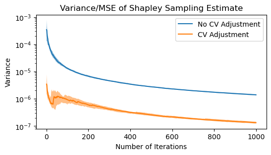
Figure 1: Variance (or MSE) of Shapley estimates. Assuming independent features, computed Shapley sampling estimates on “Prev Days” feature, using logistic regression model on Portuguese Bank dataset. Bands show inner quartiles across 50 iterations.

As Figure 1 demonstrates, ControlSHAP significantly improves the variability of Shapley estimates, regardless of the number of samples drawn. For this feature - chosen because it has the highest Shapley value - adjusting the Shapley estimate consistently reduces its variance by at least 90%.

Next, we consider the improvements in variance - equivalently, in MSE - across all 5 datasets, using a variety of machine learning predictors. We calculated the variance reduction of our ControlSHAP methods by taking the sample variance of each feature’s Shapley value across 50 iterations.

$$\text{VarReduc}_{j}(x)=\frac{\Big{[}\widehat{\text{Var}}(\hat{\phi}_{j}^{\text{model}}(x))-\widehat{\text{Var}}(\hat{\phi}_{j}^{\text{CV}}(x))\Big{]}}{\widehat{\text{Var}}(\hat{\phi}_{j}^{\text{model}}(x))}.$$ (8)

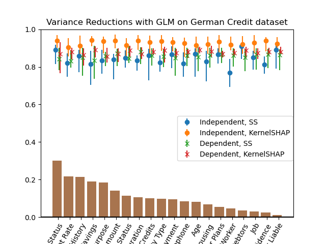
Figure 2: Variance reductions of ControlSHAP methods. Sorted features by absolute Shapley values (unscaled in plot). Confidence bands denote lower and upper quartiles of Eq. 8 across 40 held-out values of $x$.

Figure 2 displays results for all features of the German Credit dataset, using logistic regression as a predictor. Our four ControlSHAP methods produce large variance reductions on all features, whose Shapley values span several orders of magnitude. On average, our final Shapley estimates have roughly 80-95% lower variability than the original estimates.

A second stability metric we used was the number of ranking changes. This metric is motivated by the fact that often practitioners care more about identifying features with high Shapley values than the values themselves Ghorbani and Zou (2020); Narayanam and Narahari (2008); Goli and Mohammadi (2022). Formally, let $\hat{r}_{j}(x)$ be the ranking of feature $j$ within a set of $d$ Shapley estimates. For each method, we compute the average number of pairwise ranking changes across 50 resamplings.

$$\text{RankChgs}(x)={50\choose 2}^{-1}\sum_{a\neq b}\Big{[}\sum_{j=1}^{d}|\hat{r}_{j}^{a}(x)-\hat{r}_{j}^{b}(x)|\Big{]}.$$ (9)

Figure 3 shows the average number of ranking changes for 40 sample inputs. We observe that the rankings are significantly more stable with the control variate. ControlSHAP averages around 20 rank changes, compared to 60 for the original estimates. Note that this statistic highly depends on the stability of Shapley sampling prior to using control variates: if the original estimates exhibit no ranking changes between simulations, this statistic will not show an improvement even if they variance of the estimates is reduced. We believe our simulations to be representative of current practice where a noticeable reduction is evident.

Figure 3: Histogram of Ranking Changes (Eq. 9). Shapley values estimated via KernelSHAP with dependent features.

Table 1: ControlSHAP Percent Reductions in Variance (left) and Ranking Changes (right). Shapley Sampling (SS) and KernelSHAP, with and without independence assumption. Averaging variance and rank-change reductions over 40 sample inputs. Taking median variance reduction of features with 5 highest Shapley values.

Logistic Regression	SIM	BANK	BRCA	CENSUS	CREDIT
Independent Features, SS	10% $|$ 6%	76% $|$ 57%	75% $|$ 57%	33% $|$ 13%	83% $|$ 60%
Independent Features, KernelSHAP	24% $|$ 17%	84% $|$ 43%	87% $|$ 54%	3%   $|$ 2%	94% $|$ 67%
Dependent Features, SS	59% $|$ 32%	67% $|$ 42%	92% $|$ 68%	71% $|$ 58%	85% $|$ 64%
Dependent Features, KernelSHAP	51% $|$ 27%	69% $|$ 29%	94% $|$ 71%	59% $|$ 30%	87% $|$ 59%

Neural Network	SIM	BANK	BRCA	CENSUS	CREDIT
Independent Features, SS	9%   $|$ 6%	8%   $|$ 2%	76% $|$ 52%	4%   $|$ 3%	55% $|$ 36%
Independent Features, KernelSHAP	22% $|$ 15%	25% $|$ 8%	86% $|$ 55%	-1%  $|$ 1%	80% $|$ 45%
Dependent Features, SS	58% $|$ 31%	58% $|$ 37%	92% $|$ 65%	61% $|$ 42%	84% $|$ 61%
Dependent Features, KernelSHAP	51% $|$ 28%	40% $|$ 13%	92% $|$ 68%	51% $|$ 24%	87% $|$ 60%

Random Forests	SIM	BANK	BRCA	CENSUS	CREDIT
Independent Features, SS	31% $|$ 15	18% $|$ 3%	19% $|$ 7%	4%  $|$ 2%	15% $|$ 6%
Independent Features, KernelSHAP	37% $|$ 19%	4%   $|$ 3%	14% $|$ 6%	7%  $|$ 4%	14% $|$ 6%
Dependent Features, SS	56% $|$ 31%	6%   $|$ 5%	22% $|$ 11%	2%  $|$ 5%	24% $|$ 17%
Dependent Features, KernelSHAP	54% $|$ 31%	1%   $|$ -2%	17% $|$ 9%	3%  $|$ -1%	22% $|$ 10%

Table 1 contains results across all 5 datasets with logistic regression, neural network, and random forest predictors. In addition to reductions in variance, we also present reductions in the number of rank changes, averaged over 40 sample inputs. Full sets of visualizations for variance reductions and rank changes can be found in Section 2 of the appendix.

In every setting, ControlSHAP reduces the variability of Shapley estimates, often by a wide margin. For both logistic regression and neural networks, at least one ControlSHAP method produces over a 50% reduction in variance and 30% reduction in number of rank changes on all five datasets. On the BRCA and German credit datasets, these figures rise to 85% and 55% for most ControlSHAP methods. Every ControlSHAP method reduces variance by over 67% on three of the four real-world datasets with logistic regression.

While ControlSHAP is generally strong for neural networks, it tends to work better when in the dependent features case. On the simulated, bank, and census datasets, variance reductions are typically below 25% assuming independence and above 50% otherwise. Presumably, this owes to the fact that neural networks are less smooth. The quadratic model from the independent features case (Thm. 1) is more prone to neural networks’ steep gradients and hessians, and may poorly approximate model behavior as a result.

When the machine learning model is not differentiable, gradients and hessians can be taken via finite differencing. These coarse estimates use a smooth approximation to step-wise constant model behavior, which also results in a lower correlation between our target and control variate.

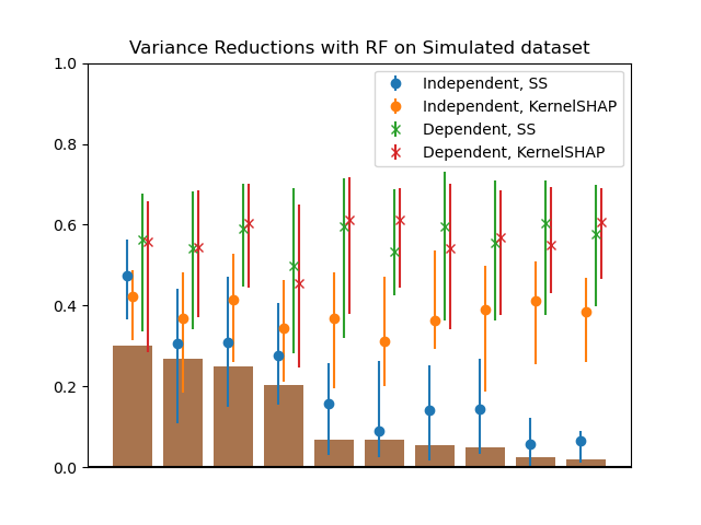
Figure 4: Variance Reductions of Random Forest on simulated dataset. Computed gradients via finite differencing.

Nevertheless, ControlSHAP increases stability on random forests, again particularly in the dependent features case. Figure 4 showcases its solid performance on the simulated dataset, reducing variability by over 50% with dependent features. Table 1 shows its reductions in variance and rank changes on all datasets and ControlSHAP methods.

6 Discussion

While Shapley values are capable of providing useful model explanations, they fall short in one critical way: stability. Stability is necessary to instill trust in our interpretations of black-box machine learning algorithms. Practitioners cannot use such a system with confidence if rerunning the same procedure yields different explanations.

This work proposes a method, ControlSHAP, to address this. ControlSHAP can be applied in conjunction with other attempts to mitigate sampling variability. Further, while designed for differentiable models, it can help explain other predictive models via finite differencing. Specifically, it adjusts Shapley estimates using the method of control variates, which track the extent to which the random samples over- or underestimate on a correlated estimator.

ControlSHAP stabilizes Shapley estimates across a wide range of datasets and algorithms, in some cases reducing variability by as high as 90%. Moreover, we can easily obtain accurate estimates of the added benefit from performing ControlSHAP adjustments. Recall that ControlSHAP reduces variance by approximately $\rho^{2}(\hat{\phi}_{j}(x)^{\text{model}},\hat{\phi}_{j}(x)^{\text{approx}})$ (Eq. 7). We can estimate this correlation using the variance and covariance used to compute $\widehat{\alpha}$; this enables us to estimate the variance reduction. As section 3 in the appendix demonstrates, these anticipated reductions closely mirror the empirical quantities.

Alternatively, ControlSHAP can be used to accelerate convergence. Covert and Lee (2020), for example, suggest terminating when the variability falls below a certain threshold. Using the control variate here could lead to a dramatic speed-up. Note in Figure 1 that the ControlSHAP estimates have comparable variability after 100 iterations as the original values after 1000.

ControlSHAP can be employed as a relatively “off-the-shelf” tool, in the sense that it stabilizes Shapley estimates with close to no extra computational or modeling work. The only model insight required is the gradient, as well as the hessian in the independent features case. Computationally, the single substantial cost is in the dependent features case, which requires accurate estimation of pre-compute matrices. Otherwise, ControlSHAP only necessitates passing each $X|X_{S}$ through the Taylor approximation, and computing the Shapley values’ covariance - both of which are extremely quick tasks.

It is worth noting that other explanation algorithms also suffer from various forms of instability. Zhou et al. (2021) and Zhou et al. (2018) found that the explanations from LIME and distillation trees are sensitive to the synthetic data used to generate them. In addition, counterfactual explanations for adjacent points may be subject to vary widely (Laugel et al., 2019).

These drawbacks motivate future work stabilizing model explanations. Shapley computations may benefit from tuning finite differences, more sophisticated Monte Carlo schemes, or alternative control variates. In some contexts it may be preferable to use inherently interpretable models like decision trees or the LASSO (Rudin, 2019; Tibshirani, 1996). We intend ControlSHAP to complement these models, enabling more trustworthy use of black-box methods.

 

Appendix

 

1 Exact Shapley Values

1.1 Shapley Value, Assuming Feature Independence

Proof.

Assume features are sampled independently in the value function. Consider a second-order Taylor approximation to $f$ at $x$:

$$g(x^{\prime}):=f(x)+(x^{\prime}-x)^{T}\nabla f(x)+\frac{1}{2}(x^{\prime}-x)^{T}\nabla^{2}f(x)(x^{\prime}-x).$$

Let $J=\nabla f(x)$, $H=\nabla^{2}f(x)$, $\Sigma=\text{Cov}(X)$, and $\sigma^{2}_{k\ell}=\text{Cov}(X_{k},X_{\ell})$. The Shapley value function is

$$v_{x}(S) =E[g(X^{\prime})|X^{\prime}_{S}=x_{S}]$$

$$=f(x)+E[(x^{\prime}-x)|X^{\prime}_{S}=x_{S}]^{T}\nabla f(x)$$

$$\qquad\qquad+\frac{1}{2}E\Big{[}(x^{\prime}-x)^{T}\nabla^{2}f(x)(x^{\prime}-x)|X^{\prime}_{S}=x_{S}\Big{]}$$

$$=f(x)+(\mu_{S^{C}}-x_{S^{C}})^{T}J_{S^{C}}$$

$$\qquad\qquad+\frac{1}{2}E\Big{[}(x_{S^{C}}^{\prime}-x_{S^{C}})^{T}\nabla^{2}f(x)_{{S^{C}}{S^{C}}}(x_{S^{C}}^{\prime}-x_{S^{C}})\Big{]},$$

where the quadratic term is equal to

$$tr(H_{{S^{C}}{S^{C}}}\Sigma_{{S^{C}}{S^{C}}})+(\mu_{S^{C}}-x_{S^{C}})^{T}H_{{S^{C}}{S^{C}}}(\mu_{S^{C}}-x_{S^{C}})$$

$$= \sum_{k\in{S^{C}}}\sum_{\ell\in{S^{C}}}H_{k\ell}\Big{(}\sigma^{2}_{k\ell}+(\mu_{k}-x_{k})(\mu_{\ell}-x_{\ell})\Big{)}$$

$$= H_{jj}(\sigma^{2}_{jj}+(\mu_{j}-x_{j})^{2}).$$

Recall $\displaystyle\phi_{j}(x):=\frac{1}{d}\sum_{S\subseteq[d]\backslash\{j\}}{d-1\choose|S|}^{-1}\big{(}v_{x}(S\cup\{j\})-v_{x}(S)\big{)}$. The difference in value functions is

$$v_{x}(S\cup j)-v_{x}(S) =\underbrace{(x_{j}-\mu_{j})J_{j}-\frac{1}{2}H_{j}j\Big{(}\sigma^{2}_{j}+(\mu_{j}-x_{j})^{2}\Big{)}}_{\leavevmode\hbox to5.02pt{\vbox to5.02pt{\text{[drawing]}}}}$$

$$\qquad\qquad-\underbrace{\sum_{k\in(S\cup j)^{C}}\underbrace{H_{jk}\Big{[}\sigma^{2}_{jk}+(\mu_{j}-x_{j})(\mu_{k}-x_{k}))\Big{]}}_{\leavevmode\hbox to4.73pt{\vbox to4.73pt{\text{[drawing]}}}}}_{\leavevmode\hbox to6.62pt{\vbox to6.62pt{\text{[drawing]}}}}.$$

Define the Shapley weight $w_{S}=\frac{1}{d}{d-1\choose|S|}^{-1}$.

$$\begin{split}\phi_{j}(x)&=\sum_{S\subseteq[d]\backslash\{j\}}w_{S}(\leavevmode\hbox to7pt{\vbox to7pt{\text{[drawing]}}}-\leavevmode\hbox to9.29pt{\vbox to9.29pt{\text{[drawing]}}})\\ &=\leavevmode\hbox to7pt{\vbox to7pt{\text{[drawing]}}}\sum_{S\subseteq[d]\backslash\{j\}}w_{S}-\sum_{S\subseteq[d]\backslash\{j\}}w_{S}\leavevmode\hbox to9.29pt{\vbox to9.29pt{\text{[drawing]}}}\\ \sum_{S\subseteq[d]\backslash\{j\}}w_{S}\leavevmode\hbox to9.29pt{\vbox to9.29pt{\text{[drawing]}}}&=\sum_{S\subseteq[d]\backslash\{j\}}w_{S}\sum_{k\in\{S\cup j\}^{C}}\leavevmode\hbox to6.58pt{\vbox to6.58pt{\text{[drawing]}}}\\ &=\sum_{S\subseteq[d]\backslash\{j\}}\sum_{k\in\{S\cup j\}^{C}}w_{S}\leavevmode\hbox to6.58pt{\vbox to6.58pt{\text{[drawing]}}}\\ &=\sum_{k\neq j}\sum_{S\subseteq[d]\backslash\{j,k\}}w_{S}\leavevmode\hbox to6.58pt{\vbox to6.58pt{\text{[drawing]}}}\\ &=\sum_{k\neq j}\leavevmode\hbox to6.58pt{\vbox to6.58pt{\text{[drawing]}}}\sum_{S\subseteq[d]\backslash\{j,k\}}w_{S}.\end{split}$$ (10)

Noting subsets of equal size have the same Shapley weight, we can easily show $\displaystyle\sum_{S\subseteq[d]\backslash\{j\}}w_{S}=1$.

$$\begin{split}\sum_{S\subseteq[d]\backslash\{j\}}w_{S}&=\sum_{S\subseteq[d]\backslash\{j\}}\frac{1}{d}{d-1\choose|S|}^{-1}\\ &=\sum_{a=0}^{d-1}{d-1\choose a}\frac{1}{d}{d-1\choose a}^{-1}=\sum_{a=0}^{d-1}\frac{1}{d}=1\end{split}$$ (11)

With a bit more arithmetic, we can show $\displaystyle\sum_{S\subseteq[d]\backslash\{j,k\}}w_{S}=\frac{1}{2}$.

$$\begin{split}\sum_{S\subseteq[d]\backslash\{j,k\}}w_{S}&=\sum_{a=0}^{d-2}{d-2\choose a}\frac{1}{d}{d-1\choose a}^{-1}\\ &=\sum_{a=0}^{d-2}\frac{(d-2)!}{a!(d-a-2)!}\frac{a!(d-a-1)!}{d!}\\ &=\sum_{a=0}^{d-2}\frac{d-a-1}{d(d-1)}\\ &=\frac{1}{d(d-1)}\Big{[}d(d-1)-\sum_{a=0}^{d-2}(a+1)\Big{]}\\ &=\frac{1}{d(d-1)}\Big{[}d(d-1)-\frac{d(d-1)}{2}\Big{]}=\frac{1}{2}.\end{split}$$ (12)

Plugging the results of 11 and 12 into 10 yields the final expression for the Shapley value:

$$\phi_{j}(x) =\leavevmode\hbox to7pt{\vbox to7pt{\text{[drawing]}}}\sum_{S\subseteq[d]\backslash\{j\}}w_{S}-\sum_{S\subseteq[d]\backslash\{j\}}w_{S}\leavevmode\hbox to9.29pt{\vbox to9.29pt{\text{[drawing]}}}$$

$$=\leavevmode\hbox to7pt{\vbox to7pt{\text{[drawing]}}}-\frac{1}{2}\sum_{k\neq j}\leavevmode\hbox to6.58pt{\vbox to6.58pt{\text{[drawing]}}}$$

$$=(x_{j}-\mu_{j})J_{j}-\frac{1}{2}H_{j}j\Big{(}\sigma^{2}_{j}+(\mu_{j}-x_{j})\Big{)}$$

$$\qquad\qquad-\frac{1}{2}\sum_{k\neq j}H_{jk}\Big{[}\sigma^{2}_{jk}+(\mu_{j}-x_{j})(\mu_{k}-x_{k}))\Big{]}$$

$$=(x_{j}-\mu_{j})J_{j}-\frac{1}{2}\Big{[}\sum_{k=1}^{d}(x_{k}-\mu_{k})H_{jk})\Big{]}(x_{j}-\mu_{j})$$

$$\qquad\qquad-\frac{1}{2}\sum_{k=1}^{d}\sigma^{2}_{jk}H_{jk}.$$

∎

1.2 Shapley Value, Correlated Features

Consider the linear model $g(x^{\prime})=\beta^{T}x^{\prime}+b$, where $x^{\prime}\sim\mathcal{N}(\mu,\Sigma)$. (For our problem, $\beta=\nabla f(x)$ and $b=f(x)$.)

Let $P_{S}$ be the projection matrix selecting set $S$; define $R_{S}=P_{\bar{S}}^{T}P_{\bar{S}}\Sigma P_{S}^{T}(P_{S}\Sigma P_{S}^{T})^{-1}P_{S}$ and $Q_{S}=P_{S}^{T}P_{S}$. We consider the set of permutations of $[d]$, each of which indexes a subset $S$ as the features that appear before $j$. Averaging over all such permutations, the Shapley values of $g(x)$ (Lundberg and Lee, 2017; Chen et al., 2020; Aas et al., 2021) are

$$\phi_{j}(x^{\prime}) =\beta\underbrace{\left[\frac{1}{d!}\sum_{m}([Q_{\{S^{m}\cup j\}^{C}}-R_{S^{m}\cup j}]-[Q_{\{S^{m}\}^{C}}-R_{S^{m}}])\right]}_{C_{j}}\mu$$

$$\qquad\qquad+\beta\underbrace{\left[\frac{1}{d!}\sum_{m}([Q_{S^{m}\cup j}+R_{S^{m}\cup j}]-[Q_{S^{m}}+R_{S^{m}}])\right]}_{D_{j}}x^{\prime}.$$

Lastly, we observe that $C_{j}=-D_{j}$. For each subset $S$, the $R$ terms cancel out; $Q_{S^{C}}+Q_{S}=I_{d}$, so $Q_{\{S\cup j\}^{C}}-Q_{S^{C}}=-(Q_{S\cup j}-Q_{S})$. This yields our expression for the dependent Shapley value:

$$\phi_{j}^{g}(x)=\beta^{T}D_{j}(x-\mu).$$

2 Comprehensive Results

We display results across all 5 datasets and 3 machine learning predictors. All datasets were binary classification problems, so we used the same models to fit them. For logistic regression and random forest, we used the sklearn implementation with default hyperparameters. For the neural network, we fit a two-layer MLP in Pytorch with 50 neurons in the hidden layer and hyperbolic tangent activation functions.

Figure 5 displays the variance reductions of our ControlSHAP methods in the four settings: Independent vs Dependent Features, and Shapley Sampling vs KernelSHAP. The error bars span the 25^th to 75^th percentiles of the variance reductions for 40 held-out samples.

Figure 6 compares the average number of changes in rankings between the original and ControlSHAP Shapley estimates. Specifically, we look the Shapley estimates obtained via KernelSHAP, assuming dependent features.

(a) Logistic Regression

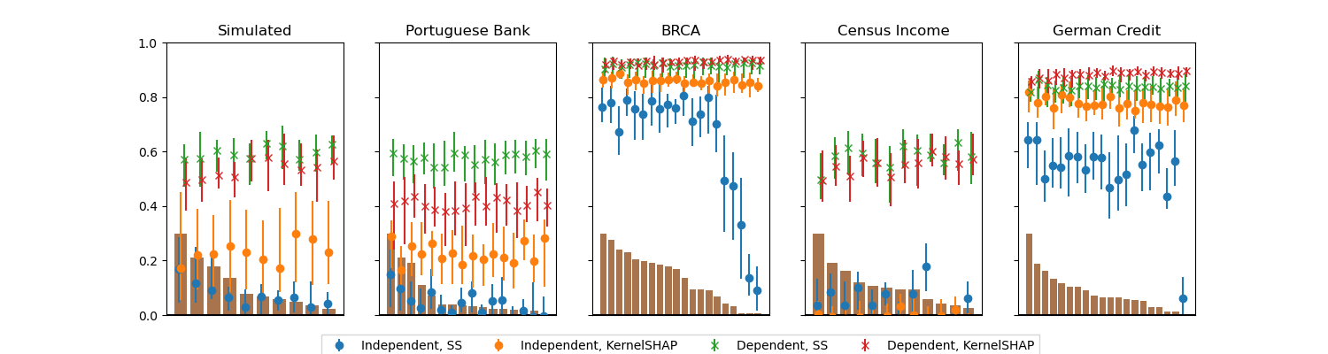
(b) Neural Network

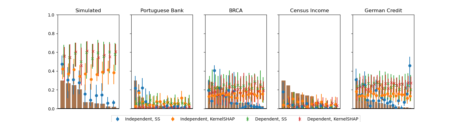
(c) Random Forest

Figure 5: Variance Reductions

(a) Logistic Regression

(b) Neural Network

(c) Random Forest

Figure 6: Average Number of Rank Changes

3 Anticipated Correlation

Figure 7 compares the observed and anticipated variance reductions, across two combinations of dataset and predictor. Recall that the variance reduction of the control variate estimate for $\phi_{j}(x)$ is $\rho^{2}(\hat{\phi}_{j}(x)^{\text{model}},\hat{\phi}_{j}(x)^{\text{approx}})$, where $\rho$ is the Pearson’s correlation coefficient. We compute the sample correlation coefficient of the Shapley values on sample $x$ as follows:

$$\hat{\rho}:=\frac{\widehat{\text{Cov}}(\hat{\phi}_{j}(x)^{\text{model}},\hat{\phi}_{j}(x)^{\text{approx}})}{\sqrt{\widehat{\text{Var}}(\hat{\phi}_{j}(x)^{\text{model}})\widehat{\text{Var}}(\hat{\phi}_{j}(x)^{\text{approx}})}}$$

We average this across the 50 iterations to obtain a single estimate for the correlation $\hat{\rho}$. The plots display the median and error bars for $\hat{\rho}^{2}(\hat{\phi}_{j}(x)^{\text{model}},\hat{\phi}_{j}(x)^{\text{approx}})$ across 40 samples. Once again, the error bars span the 25^th to 75^th percentiles.

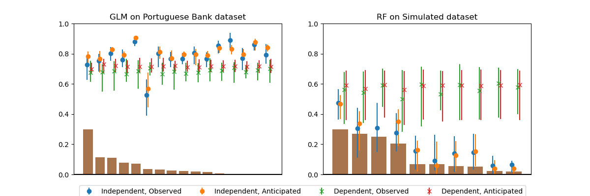
(a) Shapley Sampling

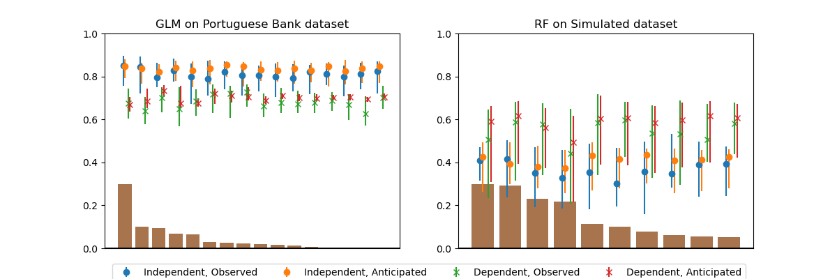
(b) KernelSHAP, Least Squares Variance Estimation

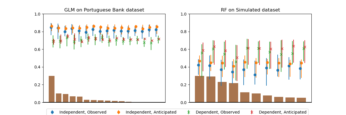
(c) KernelSHAP, Bootstrapped Variance Estimation

Figure 7: Anticipated vs Observed Variance Reduction

4 Comparing KernelSHAP Variance Estimators

Section 4.2 of the paper details methods for computing the variance and covariance between KernelSHAP estimates. Bootstrapping and the least squares covariance produce extremely similar estimates. In turn, these produce ControlSHAP estimates that reduce variance by roughly the same amount, as shown in Figure 8. This indicates that both methods are appropriate choices.

In contrast, we were not able to get the grouped method to reliably work. Its ControlSHAP estimates were often significantly more variable than the original KernelSHAP values themselves. On the bank dataset, for example, we observed several features whose ControlSHAP estimates had 7x higher variance, on average.

We ran the grouped method on 1000 iterations with a group size of 50. Following Covert and Lee (2020), we attempted to fit KernelSHAP on these 20 groups; this failed on some groups, when the problem required inverting a singular matrix. We took the sample variance and covariance of these Shapley estimates, scaling appropriately. The values we obtained ranged widely. This is sensible, as these sample variances are drawn from a heavy-tailed $\chi^{2}(19)$ sampling distribution.

Figure 9 illustrates this instability. We plot 50 random calculations of the sample Pearson correlation coefficient between the Shapley estimates of the model and Taylor approximation. The least squares method produces relatively stable estimates of correlation, and thus of variance and covariance. (Recall the correlation coefficient is the covariance divided by the product of standard deviations.) Meanwhile, the grouped method produces a much wider range of values, indicating its capacity for large errors.

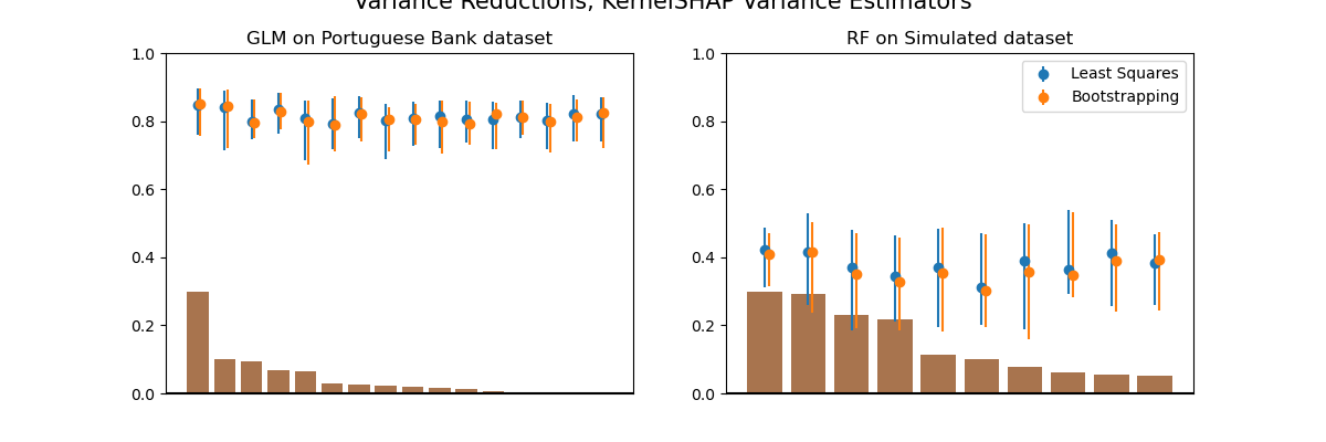
Figure 8: Variance reductions of ControlSHAP across 40 samples with bootstrapped and least-squares estimates of KernelSHAP variance and covariance. Shapley estimates computed assuming independent features.

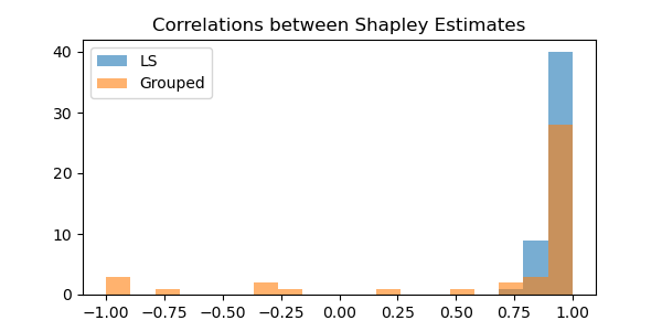
Figure 9: Grouped estimates of correlation between model and Taylor approximation. Same feature across 50 iterations, with logistic regression on the bank dataset.

References

- Aas et al. (2021) K. Aas, M. Jullum, and A. Løland. Explaining individual predictions when features are dependent: More accurate approximations to shapley values. Artif. Intell., 298:103502, 2021.
- Belle and Papantonis (2021) V. Belle and I. Papantonis. Principles and practice of explainable machine learning. Frontiers Big Data, 4:688969, 2021.
- Berger et al. (2018) A. Berger, A. Korkut, R. S. Kanchi, T. P.-G. Group, G. B. Mills, D. A. Levine, and R. Akbani. A comprehensive tcga pan-cancer molecular study of gynecologic and breast cancers. Cancer Cell, 33, 2018.
- Berk (2019) R. Berk. Machine Learning Risk Assessments in Criminal Justice Settings. Springer, 2019.
- Breiman (2001) L. Breiman. Random forests. Mach. Learn., 45(1):5–32, 2001.
- Campbell et al. (2022) T. W. Campbell, H. Roder, R. W. Georgantas III, and J. Roder. Exact shapley values for local and model-true explanations of decision tree ensembles. Machine Learning with Applications, 9:100345, 2022.
- Charnes et al. (1988) A. Charnes, B. Golany, M. Keane, and J. Rousseau. Extremal principle solutions of games in characteristic function form: core, Chebychev and Shapley value generalizations, pages 123–133. Springer, 1988.
- Chen et al. (2020) H. Chen, J. D. Janizek, S. M. Lundberg, and S. Lee. True to the model or true to the data? CoRR, abs/2006.16234, 2020.
- Chen et al. (2018) J. Chen, L. Song, M. J. Wainwright, and M. I. Jordan. L-shapley and c-shapley: Efficient model interpretation for structured data. CoRR, abs/1808.02610, 2018.
- Covert and Lee (2020) I. Covert and S. Lee. Improving kernelshap: Practical shapley value estimation via linear regression. CoRR, abs/2012.01536, 2020.
- Covert et al. (2020) I. Covert, S. M. Lundberg, and S. Lee. Understanding global feature contributions through additive importance measures. CoRR, abs/2004.00668, 2020.
- Dubey and Chandani (2022) R. Dubey and A. Chandani. Application of machine learning in banking and finance: a bibliometric analysis. Int. J. Data Anal. Tech. Strateg., 14(3), 2022.
- Fang et al. (1990) K.-T. Fang, S. Kotz, and K. W. Ng. Symmetric Multivariate and Related Distributions. Chapman and Hall, 1990.
- Ferdous et al. (2020) M. Ferdous, J. Debnath, and N. R. Chakraborty. Machine learning algorithms in healthcare: A literature survey. In 11th International Conference on Computing, Communication and Networking Technologies, ICCCNT 2020, Kharagpur, India, July 1-3, 2020, pages 1–6. IEEE, 2020.
- Ghorbani and Zou (2020) A. Ghorbani and J. Y. Zou. Neuron shapley: Discovering the responsible neurons. In H. Larochelle, M. Ranzato, R. Hadsell, M. Balcan, and H. Lin, editors, Advances in Neural Information Processing Systems 33: Annual Conference on Neural Information Processing Systems 2020, NeurIPS 2020, December 6-12, 2020, virtual, 2020.
- Goli and Mohammadi (2022) A. Goli and H. Mohammadi. Developing a sustainable operational management system using hybrid Shapley value and Multimoora method: case study petrochemical supply chain. Environment, Development and Sustainability: A Multidisciplinary Approach to the Theory and Practice of Sustainable Development, 24(9):10540–10569, September 2022. doi: 10.1007/s10668-021-01844-.
- Hofmann (1994) H. Hofmann. Statlog (german credit data), Nov. 1994.
- Hooker et al. (2021) G. Hooker, L. Mentch, and S. Zhou. Unrestricted permutation forces extrapolation: variable importance requires at least one more model, or there is no free variable importance. Statistics and Computing, 31:1–16, 2021.
- Jethani et al. (2022) N. Jethani, M. Sudarshan, I. C. Covert, S. Lee, and R. Ranganath. Fastshap: Real-time shapley value estimation. In The Tenth International Conference on Learning Representations, ICLR 2022, Virtual Event, April 25-29, 2022. OpenReview.net, 2022.
- Kohavi (1996) R. Kohavi. Census income, Apr. 1996.
- Laugel et al. (2019) T. Laugel, M. Lesot, C. Marsala, and M. Detyniecki. Issues with post-hoc counterfactual explanations: a discussion. CoRR, abs/1906.04774, 2019. URL http://arxiv.org/abs/1906.04774.
- Leisch et al. (1970) F. Leisch, A. Weingessel, and K. Hornik. On the generation of correlated artificial binary data. SFB Adaptive Information Systems and Modelling in Economics and Management Science, 20, 02 1970.
- Lundberg and Lee (2017) S. M. Lundberg and S. Lee. A unified approach to interpreting model predictions. In I. Guyon, U. von Luxburg, S. Bengio, H. M. Wallach, R. Fergus, S. V. N. Vishwanathan, and R. Garnett, editors, Advances in Neural Information Processing Systems 30: Annual Conference on Neural Information Processing Systems 2017, December 4-9, 2017, Long Beach, CA, USA, pages 4765–4774, 2017.
- Lundberg et al. (2020) S. M. Lundberg, G. G. Erion, H. Chen, A. J. DeGrave, J. M. Prutkin, B. Nair, R. Katz, J. Himmelfarb, N. Bansal, and S. Lee. From local explanations to global understanding with explainable AI for trees. Nat. Mach. Intell., 2(1):56–67, 2020. doi: 10.1038/s42256-019-0138-9. URL https://doi.org/10.1038/s42256-019-0138-9.
- Mandalapu et al. (2023) V. Mandalapu, L. Elluri, P. Vyas, and N. Roy. Crime prediction using machine learning and deep learning: A systematic review and future directions. IEEE Access, 11:60153–60170, 2023.
- Mitchell et al. (2022) R. Mitchell, J. Cooper, E. Frank, and G. Holmes. Sampling permutations for shapley value estimation. J. Mach. Learn. Res., 23:43:1–43:46, 2022.
- Moro et al. (2014) S. Moro, P. Cortez, and P. Rita. A data-driven approach to predict the success of bank telemarketing. Decis. Support Syst., 62:22–31, 2014.
- Narayanam and Narahari (2008) R. Narayanam and Y. Narahari. Determining the top-k nodes in social networks using the shapley value. In L. Padgham, D. C. Parkes, J. P. Müller, and S. Parsons, editors, 7th International Joint Conference on Autonomous Agents and Multiagent Systems (AAMAS 2008), Estoril, Portugal, May 12-16, 2008, Volume 3, pages 1509–1512. IFAAMAS, 2008.
- Oates et al. (2017) C. J. Oates, M. Girolami, and N. Chopin. Control functionals for monte carlo integration. Journal of the Royal Statistical Society Series B: Statistical Methodology, 79(3):695–718, 2017.
- Ribeiro et al. (2016) M. T. Ribeiro, S. Singh, and C. Guestrin. ”why should I trust you?”: Explaining the predictions of any classifier. In B. Krishnapuram, M. Shah, A. J. Smola, C. C. Aggarwal, D. Shen, and R. Rastogi, editors, Proceedings of the 22nd ACM SIGKDD International Conference on Knowledge Discovery and Data Mining, San Francisco, CA, USA, August 13-17, 2016, pages 1135–1144. ACM, 2016.
- Rudin (2019) C. Rudin. Stop explaining black box machine learning models for high stakes decisions and use interpretable models instead. Nat. Mach. Intell., 1(5):206–215, 2019. doi: 10.1038/s42256-019-0048-x. URL https://doi.org/10.1038/s42256-019-0048-x.
- Shapley (1952) L. Shapley. A value for n-person games, march 1952.
- Song et al. (2016) E. Song, B. L. Nelson, and J. Staum. Shapley effects for global sensitivity analysis: Theory and computation. SIAM/ASA J. Uncertain. Quantification, 4(1):1060–1083, 2016.
- Strumbelj and Kononenko (2010) E. Strumbelj and I. Kononenko. An efficient explanation of individual classifications using game theory. J. Mach. Learn. Res., 11:1–18, 2010.
- Strumbelj and Kononenko (2014) E. Strumbelj and I. Kononenko. Explaining prediction models and individual predictions with feature contributions. Knowl. Inf. Syst., 41(3):647–665, 2014.
- Tibshirani (1996) R. Tibshirani. Regression shrinkage and selection via the lasso. Journal of the Royal Statistical Society. Series B (Methodological), 58(1):267–288, 1996. ISSN 00359246.
- Tomita et al. (2020) T. M. Tomita, J. Browne, C. Shen, J. Chung, J. L. Patsolic, B. Falk, C. E. Priebe, J. Yim, R. Burns, M. Maggioni, et al. Sparse projection oblique randomer forests. The Journal of Machine Learning Research, 21(1):4193–4231, 2020.
- Verma et al. (2020) S. Verma, J. P. Dickerson, and K. Hines. Counterfactual explanations for machine learning: A review. CoRR, abs/2010.10596, 2020.
- Zhou et al. (2018) Y. Zhou, Z. Zhou, and G. Hooker. Approximation trees: Statistical stability in model distillation. CoRR, abs/1808.07573, 2018. URL http://arxiv.org/abs/1808.07573.
- Zhou et al. (2021) Z. Zhou, G. Hooker, and F. Wang. S-LIME: stabilized-lime for model explanation. In F. Zhu, B. C. Ooi, and C. Miao, editors, KDD ’21: The 27th ACM SIGKDD Conference on Knowledge Discovery and Data Mining, Virtual Event, Singapore, August 14-18, 2021, pages 2429–2438. ACM, 2021. doi: 10.1145/3447548.3467274. URL https://doi.org/10.1145/3447548.3467274.