Polytopal discontinuous Galerkin discretization of brain multiphysics flow dynamics

Abstract

A comprehensive mathematical model of the multiphysics flow of blood and Cerebrospinal Fluid (CSF) in the brain can be expressed as the coupling of a poromechanics system and Stokes’ equations: the first describes fluids filtration through the cerebral tissue and the tissue’s elastic response, while the latter models the flow of the CSF in the brain ventricles. This model describes the functioning of the brain’s waste clearance mechanism, which has been recently discovered to play an essential role in the progress of neurodegenerative diseases. To model the interactions between different scales in the porous medium, we propose a physically consistent coupling between Multi-compartment Poroelasticity (MPE) equations and Stokes’ equations. In this work, we introduce a numerical scheme for the discretization of such coupled MPE-Stokes system, employing a high-order discontinuous Galerkin method on polytopal grids to efficiently account for the geometric complexity of the domain. We analyze the stability and convergence of the space semidiscretized formulation, we prove a-priori error estimates, and we present a temporal discretization based on a combination of Newmark’s $\beta$-method for the elastic wave equation and the $\theta$-method for the other equations of the model. Numerical simulations carried out on test cases with manufactured solutions validate the theoretical error estimates. We also present numerical results on a two-dimensional slice of a patient-specific brain geometry reconstructed from diagnostic images, to test in practice the advantages of the proposed approach.

Keywords – Cerebrospinal fluid, Stokes’ equation, Multiple-Network Poroelasticity Theory, Polygonal/polyhedral mesh, Multiphysics system

1 Introduction

In the brain, multiple fluid components play different roles: the blood supplies nutrients and oxygen and removes carbon dioxide, while the Cerebrospinal Fluid (CSF) and the glymphatic system [61, 51, 22] have the primary function of clearing the waste produced by brain activity. Also, it has been recently shown that waste clearance mechanisms play a major role in the evolution of neurodegenerative diseases [15, 55, 50, 24]. These physical systems are strongly interconnected with one another and with the cerebral matter: for example, a large amount of the CSF is generated in the choroid plexus thanks to the high concentration of blood capillary vessels in it [25]; also, an auxiliary function of the CSF is to protect the brain from impact against the skull and to compensate blood pulsatility in terms of flow rate and pressure inside the braincase. For this reason, the modeling of the fluid dynamics in the brain requires a multiphysics perspective, able to capture these interactions and their mutual interplay.

From the modeling viewpoint, the brain can be described as a porous material (white and gray matter) with fluids both filtrating through it and flowing in hollow regions (brain ventricles). In terms of mathematical modeling, this can be represented as the coupling between a poromechanics system – described, e.g., by Darcy’s or Biot’s equations [74] – and Stokes/Navier-Stokes’ equations for the flow in the ventricles [58, 48]. Numerical methods for such Fluid-Poroelastic Structure Interaction (FPSI) systems can be found in the literature: the most studied is the Biot-Stokes’ system [16, 3, 2, 23], but also more complex models have been investigated, e.g. considering a multilayer structure of the porous medium [21, 28], a non-linear constitutive model for either the structural or fluid part of the system [40], or Multi-compartment Poroelasticity (MPE) models coupled with Stokes’ equations [41, 18]. This latter framework is the best suited to model brain poromechanics and CSF flow, since it can simultaneously represent cerebral tissue deformation, blood vessel networks at different scales, CSF flow, and waste clearance. Moreover, the dynamic formulation of MPE equations can describe the inertial forces associated with blood pressure pulsatility during a heartbeat, which affects vascular and tissue deformations and waste clearance [71, 33, 39, 35].

The analysis of conforming Finite Element methods for FPSI problems has been addressed in several of the abovementioned works, with a discussion on the inf-sup requirements on the different components of the system (poroelastic, fluid, and coupling conditions). However, aiming at an accurate representation of the poromechanics and flow with low dispersion and dissipation errors, high-order discretization methods provide a better choice [66, 49]. Polytopal Discontinuous Galerkin (PolyDG) methods fit in this framework, and they can also naturally account for complex geometries such as vessel networks and brain folds, thanks to their flexibility in terms of local refinement and agglomeration, hanging nodes treatment, and generality of mesh element shapes [19, 31, 11, 30, 65, 29]. In addition, discontinuous Galerkin schemes provide a general framework to embed physically-consistent interface conditions directly in the weak form. So far, these methods have been mostly employed to solve porous media and poroelasticity problems for geophysical applications [59, 12, 10] and for fluid dynamics and fluid-structure interaction problems [34, 42, 72, 7, 73, 75, 14].

In this work, we introduce a high-order PolyDG method to spatially discretize a coupled model encompassing dynamic Multiple-Network Poroelastic (MPE) equations for poromechanics [35] and Stokes’ equations [8, 14], with physically-consistent coupling conditions inspired from the mass and stress balance at the interface between the brain tissue and the CSF. Moreover, we take full advantage of the DG framework to embed, directly in the physically consistent formulation, the coupling conditions at the interface between the poroelastic and fluid regions. We analyze the well-posedness and convergence of the semidiscrete numerical method, and we employ a combination of Newmark’s $\beta$-method and the $\theta$-method for time discretization.

The paper is organized as follows. In Section 2, we introduce the multiphysics problem, both in strong and weak form, and discuss the coupling conditions. Section 3 describes the PolyDG space discretization; stability and convergence properties are analyzed in Section 4. Then, time discretization is introduced Section 5. Verification tests are discussed in Section 6, corroborating the theoretical results of Section 4. Section 7 demonstrates the capabilities of the method on a two-dimensional brain section considering physiological settings.

2 Mathematical model

We introduce the mathematical model consisting of the coupling between a Multiple-Network Poroelasticity system and Stokes’ system: the former, introduced in [35], accounts for the poromechanics of the brain tissue and its interaction with different fluids compartments flowing in its pores, while the latter describes the flow of the CSF in the brain ventricles. To ease the presentation, we consider a simplified configuration whose two-dimensional representation is depicted in Fig. 1. The poroelastic medium occupies a portion $\Omega_{\rm el}\subset\mathbb{R}^{d}$ ($d=2,3$) of the domain, while the CSF flows according to Stokes’ equations in the remaining portion $\Omega_{\rm f}\subset\mathbb{R}^{d}$. The interaction between the two systems occurs at the interface $\Sigma=\overline{\Omega}_{\rm el}\cap\overline{\Omega}_{\rm f}$, which we suppose to be a (piecewise) smooth $(d-1)-$manifold. The source of CSF comes from an exchange of mass with the poroelastic medium and it exits from the domain at $\Gamma_{\text{out}}$, while the rest of the domain boundary is a solid wall $\Gamma_{\rm w}$. We denote by $\Omega$ the interior of $\overline{\Omega}_{\rm el}\cup\overline{\Omega}_{\rm f}$.

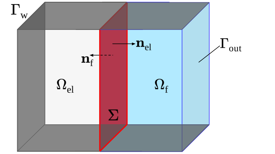
Figure 1: Domain scheme: poroelastic medium in $\Omega_{\rm el}$ (light grey), Stokes’ flow of CSF in $\Omega_{\rm f}$ (blue), interface $\Sigma$ (red), and external boundaries $\Gamma_{\rm w}$ (dark grey) and $\Gamma_{\text{out}}$.

Given a final observation time $T>0$, we introduce the CSF velocity ${\bm{u}}:\Omega_{\rm f}\times[0,T]\to\mathbb{R}^{d}$ and pressure $p:\Omega_{\rm f}\times[0,T]\to\mathbb{R}$, the solid tissue displacement ${\bm{d}}:\Omega_{\rm el}\times[0,T]\to\mathbb{R}^{d}$, and the network pressures $p_{\rm j}:\Omega_{\rm el}\times[0,T]\to\mathbb{R}$, ${\rm j}\in J$, where $J$ is a given set of labels denoting the different fluid network compartments [35]. In particular, for the application at hand, we consider $J=\{\text{A},\text{C},\text{V},{\rm E}\}$, where A, C, V correspond to the arterial, capillary, and venous blood compartments, respectively, while ${\rm E}$ denotes the extracellular CSF permeating the brain tissue.

The coupled problem reads as follows:

$$\rho_{\rm el}\partial_{tt}^{2}{\bm{d}}-\nabla\cdot\sigma_{\rm el}({\bm{d}})+\sum_{{\rm k}\in J}\alpha_{\rm k}\nabla p_{\rm k}={\bm{f}}_{\rm el}, \qquad\text{in }\Omega_{\rm el}\times(0,T],$$ (1a)

$$c_{\rm j}\partial_{t}p_{\rm j}+\nabla\cdot\left(\alpha_{\rm j}\partial_{t}{\bm{d}}-\frac{1}{\mu_{\rm j}}K_{\rm j}\nabla p_{\rm j}\right)$$ (1b)

$$\qquad+\sum_{{\rm k}\in J}\beta_{{\rm j}{\rm k}}(p_{\rm j}-p_{\rm k})+\beta_{\rm j}^{\text{e}}p_{\rm j}=g_{\rm j}, \qquad\text{in }\Omega_{\rm el}\times(0,T],\quad\forall{\rm j}\in J,$$ (1c)

$$\rho_{\rm f}\partial_{t}{\bm{u}}-\nabla\cdot\sigma_{\rm f}({\bm{u}})+\nabla p={\bm{f}}_{\rm f}, \qquad\text{in }\Omega_{\rm f}\times(0,T],$$ (1d)

$$\nabla\cdot{\bm{u}}=0, \qquad\text{in }\Omega_{\rm f}\times(0,T],$$ , (1e)

where the linear elastic and fluid (viscous) stress tensors are defined as $\sigma_{\rm el}({\bm{d}})=2\mu_{\rm el}\varepsilon({\bm{d}})+\lambda(\nabla\cdot{\bm{d}})I$ and $\sigma_{\rm f}({\bm{u}})=2\mu_{\rm f}\varepsilon({\bm{u}})$, respectively, with $\varepsilon({\bm{w}})=\left(\nabla{\bm{w}}+\nabla{\bm{w}}^{T}\right)/2,$. The body forces ${\bm{f}}_{\rm el}:\Omega_{\rm el}\times(0,T]\to\mathbb{R}^{d},g_{\rm j}:\Omega_{\rm el}\times(0,T]\to\mathbb{R},{\bm{f}}_{\rm f}:\Omega_{\rm f}\times(0,T]\to\mathbb{R}^{d}$ are supposed sufficiently regular. The parameters of the models are explained in Table 1, with their typical physiological values extracted from [57, 35, 32]. The initial and boundary conditions of problem (1e) are defined as

$$\Bigl{(}{\bm{d}}(0),\partial_{t}{\bm{d}}(0)\Bigr{)}=\Bigl{(}{\bm{d}}_{0},\dot{{\bm{d}}}_{0}\Bigr{)},\quad p_{\rm j}(0)=p_{{\rm j}0}, \qquad\text{in }\Omega_{\rm el},\quad\forall{\rm j}\in J,$$ (2a)

$${\bm{u}}(0)={\bm{u}}_{0} \qquad\text{in }\Omega_{\rm f},$$ (2b)

$${\bm{d}}={\bm{d}}_{\rm D}={\bm{0}}, \qquad\text{on }\Gamma_{\rm w}\times(0,T],$$ (2c)

$$\frac{1}{\mu_{\rm j}}K_{\rm j}\nabla p_{\rm j}\cdot{\bm{n}}_{\rm el}=0, \qquad\text{on }\Gamma_{\rm w}\times(0,T],\quad\forall{\rm j}\in J,$$ (2d)

$${\bm{u}}={\bm{u}}_{\rm D}={\bm{0}}, \qquad\text{on }\Gamma_{\rm w}\times(0,T],$$ (2e)

$$(\sigma_{\rm f}({\bm{u}})-pI){\bm{n}}_{\rm f}=-\overline{p}^{\text{out}}{\bm{n}}_{\rm f}, \qquad\text{on }\Gamma_{\text{out}}\times(0,T],$$ (2f)

with suitable definition of the data function $\overline{p}^{\text{out}}:\Gamma_{\text{out}}\times(0,T]\to\mathbb{R}$, that represents the external normal stress at the outlet, and of the initial conditions ${\bm{d}}_{0}:\Omega_{\rm el}\to\mathbb{R}^{d},\dot{{\bm{d}}}_{0}:\Omega_{\rm el}\to\mathbb{R}^{d},{\bm{u}}_{0}:\Omega_{\rm f}\to\mathbb{R}^{d},p_{{\rm j}0}:\Omega_{\rm el}\to\mathbb{R},{\rm j}\in J$.

parameter	phys. values	description
$\rho_{\rm el}$	$1000\text{\,}\mathrm{kg}\text{⋅}{\mathrm{m}}^{-3}$	density of the solid tissue
$\rho_{\rm f}$	$1000\text{\,}\mathrm{kg}\text{⋅}{\mathrm{m}}^{-3}$	density of the CSF
$\mu_{\rm el}$	$216\text{\,}\mathrm{Pa}$	first Lamé parameter of the solid
$\lambda$	$505\text{\,}\mathrm{Pa}$	second Lamé parameter of the solid
$\mu_{\rm j}$	$3.5\text{⋅}{10}^{-3}\text{\,}\mathrm{Pa}\text{⋅}\mathrm{s}$	viscosity of the fluid in compartment ${\rm j}\in J$
$\mu_{\rm f}$	$3.5\text{⋅}{10}^{-3}\text{\,}\mathrm{Pa}\text{⋅}\mathrm{s}$	viscosity of CSF
$\alpha_{\rm j}$	$\in[0,1)$	Biot-Willis coefficient of compartment ${\rm j}\in J$
$c_{\rm j}$	$1\text{⋅}{10}^{-6}\text{\,}{\mathrm{m}}^{2}\text{⋅}{\mathrm{N}}^{-1}$	storage coefficient of compartment ${\rm j}\in J$
$k_{\rm j}$	$1\text{⋅}{10}^{-11}\text{\,}{\mathrm{m}}^{2}$	$K_{\rm j}=k_{\rm j}I$ permeability tensor for compartment ${\rm j}\in J$
$\beta_{{\rm j}{\rm k}}$	$1\text{\,}{\mathrm{m}}^{2}\text{⋅}{\mathrm{N}}^{-1}\text{⋅}{\mathrm{s}}^{-1}$	coupling transfer coefficient between compartments
		(from ${\rm k}\in J$ to ${\rm j}\in J$)
$\beta_{{\rm j}}^{\text{e}}$	$1\text{\,}{\mathrm{m}}^{2}\text{⋅}{\mathrm{N}}^{-1}\text{⋅}{\mathrm{s}}^{-1}$	external coupling coefficient for compartment ${\rm j}\in J$

Table 1: Parameters of model (1e) with corresponding physiological values.

On the interface $\Sigma$, we introduce the following coupling conditions, based on physiological considerations:

$$\sigma_{\rm el}({\bm{d}}){\bm{n}}_{\rm el}-\sum_{{\rm k}\in J}\alpha_{\rm k}p_{\rm k}{\bm{n}}_{\rm el}+\sigma_{\rm f}({\bm{u}}){\bm{n}}_{\rm f}-p{\bm{n}}_{\rm f}={\bm{0}}, \quad\text{on }\Sigma\times(0,T],$$ (3a)

$$\frac{1}{\mu_{\rm j}}K_{\rm j}\nabla p_{\rm j}\cdot{\bm{n}}_{\rm el}=0, \quad\text{on }\Sigma\times(0,T],\quad\forall{\rm j}\in J\setminus\{{\rm E}\},$$ (3b)

$${\bm{u}}\cdot{\bm{n}}_{\rm f}+\left(\partial_{t}{\bm{d}}-\frac{1}{\mu_{\rm E}}K_{\rm E}\nabla p_{\rm E}\right)\cdot{\bm{n}}_{\rm el}=0, \quad\text{on }\Sigma\times(0,T],$$ (3c)

$$p_{\rm E}=p-\sigma_{\rm f}({\bm{u}}){\bm{n}}_{\rm f}\cdot{\bm{n}}_{\rm f}, \quad\text{on }\Sigma\times(0,T],$$ (3d)

$$\left(\sigma_{\rm f}({\bm{u}}){\bm{n}}_{\rm f}-p{\bm{n}}_{\rm f}\right)\wedge{\bm{n}}_{\rm f}={\bm{0}}, \quad\text{on }\Sigma\times(0,T].$$ (3e)

Condition (3a) expresses the balance of total normal stress. Due to the blood-brain barrier [1, 38], we assume that mass exchange between the poroelastic domain and the CSF only occurs through compartment ${\rm E}$, as expressed by (3b)-(3c). Consistently, the normal stress of the CSF fluid is balanced by the pressure of compartment ${\rm E}$, as in (3d), while we assume the tangential stress on the fluid to be negligible (cf. (3e)). Similar assumptions were made in [32], although we do not make use of the Beavers-Joseph-Saffman condition [64].

Aiming at solving problem (1e) with the Finite Element method, we introduce its weak formulation. For the sake of generality, let $\Gamma_{\text{D},{\bm{d}}},\Gamma_{\text{D},{\bm{u}}},\Gamma_{\text{D},P_{\rm j}}$, with ${\rm j}\in J$, denote the portions of $\partial\Omega$ where Dirichlet boundary conditions on ${\bm{d}},{\bm{u}},p_{\rm j}$ are imposed, respectively. Then, we introduce the following functional spaces:

$$\begin{gathered}{\bm{W}}=\{{\bm{w}}\in[H^{1}(\Omega_{\rm el})]^{d}\colon{\bm{w}}=0\text{ on }\Gamma_{\text{D},{\bm{d}}}\},\qquad{\bm{V}}=\{{\bm{v}}\in[H^{1}(\Omega_{\rm f})]^{d}\colon{\bm{v}}=0\text{ on }\Gamma_{\text{D},{\bm{u}}}\},\\ Q_{\rm j}=\{q_{\rm j}\in H^{1}(\Omega_{\rm el})\colon q_{\rm j}=0\text{ on }\Gamma_{\text{D},P_{\rm j}}\},\ \forall{\rm j}\in J,\qquad Q=L^{2}(\Omega_{\rm f}),\end{gathered}$$

where $H^{1}(\Omega)$ denotes the classical Sobolev space of order 1 over $L^{2}(\Omega)$. For the problem at hand, all Dirichlet boundary conditions on $\partial\Omega$ are homogenous. We denote by $(\cdot,\cdot)_{\Omega}$ the $L^{2}$-product over $\Omega$ and we define the following forms and functionals over the spaces introduced above:

$$a_{\rm el}:{\bm{W}}\times{\bm{W}}\to\mathbb{R}, \qquad a_{\rm el}({\bm{d}},{\bm{w}})=(\sigma_{\rm el}({\bm{d}}),\varepsilon({\bm{w}}))_{\Omega_{\rm el}},$$

$$a_{\rm j}:Q_{\rm j}\times Q_{\rm j}\to\mathbb{R}, \qquad a_{\rm j}(p_{\rm j},q_{\rm j})=\left(\frac{1}{\mu_{\rm j}}K_{\rm j}\nabla p_{\rm j},\nabla q_{\rm j}\right)_{\Omega_{\rm el}}\qquad\forall{\rm j}\in J,$$

$$C_{\rm j}:\left(\bigtimes_{{\rm k}\in J}Q_{\rm k}\right)\times Q_{\rm j}\to\mathbb{R}, \qquad C_{\rm j}(\{p_{\rm k}\}_{{\rm k}\in J},q_{\rm j})=\sum_{{\rm k}\in J}(\beta_{{\rm k}{\rm j}}(p_{\rm j}-p_{\rm k}),q_{\rm j})_{\Omega_{\rm el}}+(\beta_{{\rm j}}^{\text{e}}p_{\rm j},q_{\rm j})_{\Omega_{\rm el}}\qquad\forall{\rm j}\in J,$$

$$a_{\rm f}:{\bm{V}}\times{\bm{V}}\to\mathbb{R}, \qquad a_{\rm f}({\bm{u}},{\bm{v}})=(\sigma_{\rm f}({\bm{u}}),\varepsilon({\bm{v}}))_{\Omega_{\rm f}},$$

$$b_{\rm j}:Q_{\rm j}\times{\bm{W}}\to\mathbb{R}, \qquad b_{\rm j}(q_{\rm j},{\bm{w}})=-(\alpha_{\rm j}p_{\rm j},{\rm div}{\bm{w}})_{\Omega_{\rm el}}\qquad\forall{\rm j}\in J,$$

$$b_{\rm f}:Q\times{\bm{V}}\to\mathbb{R}, \qquad b_{\rm f}(q,{\bm{v}})=-(q,{\rm div}{\bm{v}})_{\Omega_{\rm f}},$$

$$F_{\rm el}:{\bm{W}}\to\mathbb{R}, \qquad F_{\rm el}({\bm{w}})=({\bm{f}}_{\rm el},{\bm{w}})_{\Omega_{\rm el}},$$

$$F_{\rm j}:Q_{\rm j}\to\mathbb{R}, \qquad F_{\rm j}(q_{\rm j})=(g_{\rm j},q_{\rm j})_{\Omega_{\rm el}}\qquad\forall{\rm j}\in J,$$

$$F_{\rm f}:{\bm{V}}\to\mathbb{R}, \qquad F_{\rm f}({\bm{v}})=({\bm{f}}_{\rm f},{\bm{v}})_{\Omega_{\rm f}},$$

$$\mathfrak{J}:Q_{\rm E}\times{\bm{W}}\times{\bm{V}}\to\mathbb{R}, \qquad\mathfrak{J}(p_{\rm E},{\bm{w}},{\bm{v}})=\int_{\Sigma}p_{\rm E}\left({\bm{w}}\cdot{\bm{n}}_{\rm el}+{\bm{v}}\cdot{\bm{n}}_{\rm f}\right)d\Sigma.$$

Remark 2.1 (Derivation of the interface form $\mathfrak{J}$)

The interface form $\mathfrak{J}:Q^{\rm DG}_{{\rm E},h}\times{\bm{W}}^{\rm DG}_{h}\times{\bm{V}}^{\rm DG}_{h}\to\mathbb{R}$ introduced above naturally arises during the derivation of the weak form of problem (1e). We test (1a)-(1c) against functions ${\bm{w}}\in{\bm{W}}$ and $q_{\rm j}\in Q_{\rm j}$, with ${\rm j}\in J$, over $\Omega_{\rm el}$, and (1d) against ${\bm{v}}\in{\bm{V}}$ over $\Omega_{\rm f}$. Then, integrating by parts and summing all the contributions yield the following boundary terms on the interface:

$$\int_{\Sigma}\left[(pI-\sigma_{\rm f}({\bm{u}}))\colon{\bm{v}}\otimes{\bm{n}}_{\rm f}+\left(\sum_{{\rm k}\in J}\alpha_{\rm k}p_{\rm k}I-\sigma_{\rm el}({\bm{d}})\right)\colon{\bm{w}}\otimes{\bm{n}}_{\rm el}-\sum_{{\rm j}\in J}\frac{1}{\mu_{\rm j}}K_{\rm j}\nabla p_{\rm j}\cdot q_{\rm j}{\bm{n}}_{\rm el}\right]d\Sigma.$$ (4)

Using the interface conditions (3a)-(3b) and then (3c)-(3d)-(3e), we can rewrite (4) as follows:

$$\int_{\Sigma} \left[(pI-\sigma_{\rm f}({\bm{u}}))\colon({\bm{v}}\otimes{\bm{n}}_{\rm f}+{\bm{w}}\otimes{\bm{n}}_{\rm el})-\frac{1}{\mu_{\rm E}}K_{\rm E}\nabla p_{\rm E}\cdot q_{\rm E}{\bm{n}}_{\rm el}\right]d\Sigma$$ (5)

$$=\int_{\Sigma}\left[p_{\rm E}({\bm{v}}\cdot{\bm{n}}_{\rm f}+{\bm{w}}\cdot{\bm{n}}_{\rm el})-q_{\rm E}({\bm{u}}\cdot{\bm{n}}_{\rm f}+\partial_{t}{\bm{d}}\cdot{\bm{n}}_{\rm el})\right]d\Sigma=\mathfrak{J}(p_{\rm E},{\bm{w}},{\bm{v}})-\mathfrak{J}(q_{\rm E},\partial_{t}{\bm{d}},{\bm{u}}),$$

where we also used that ${\bm{a}}\otimes{\bm{b}}\colon I={\bm{a}}\cdot{\bm{b}}$ for any ${\bm{a}},{\bm{b}}\in\mathbb{R}^{d}$.

Denoting by $L^{2}(0,T;H),H^{1}(0,T;H)$ the time-dependent Bochner spaces associated to a Sobolev space $H$, and setting

$$\mathscr{D}=H^{2}(0,T;{\bm{W}}),\ \ \mathscr{P}=\bigtimes_{{\rm j}\in J}H^{1}(0,T;Q_{\rm j}),\ \ \mathscr{V}=H^{1}(0,T;{\bm{V}}),\ \ \mathscr{Q}=L^{2}(0,T;Q),$$

the weak formulation of problem (1e) reads as follows:
Find $({\bm{d}},\{p_{\rm j}\}_{{\rm j}\in J},{\bm{u}},p)\in\mathscr{D}\times\mathscr{P}\times\mathscr{V}\times\mathscr{Q}$ such that, for all $t\in(0,T]$,

$$(\rho_{\rm el}\partial_{tt}^{2}{\bm{d}},{\bm{w}})_{\Omega_{\rm el}}+a_{\rm el}({\bm{d}},{\bm{w}})+\sum_{{\rm j}\in J}b_{\rm j}(p_{\rm j},{\bm{w}})-F_{\rm el}({\bm{w}})$$ (6)

$$\qquad+\sum_{{\rm j}\in J}\Bigl{[}(c_{\rm j}\partial_{t}p_{\rm j},q_{\rm j})_{\Omega_{\rm el}}+a_{\rm j}(p_{\rm j},q_{\rm j})+C_{j}(\{p_{\rm k}\}_{{\rm k}\in J},q_{\rm j})-b_{\rm j}(q_{\rm j},\partial_{t}{\bm{d}})-F_{\rm j}(q_{\rm j})\Bigr{]}$$

$$\qquad+(\rho_{\rm f}\partial_{t}{\bm{u}},{\bm{v}})_{\Omega_{\rm f}}+a_{\rm f}({\bm{u}},{\bm{v}})+b_{\rm f}(p,{\bm{v}})+b_{\rm f}(q,{\bm{u}})-F_{\rm f}({\bm{v}})$$

$$\qquad+\mathfrak{J}(p_{\rm E},{\bm{w}},{\bm{v}})-\mathfrak{J}(q_{\rm E},\partial_{t}{\bm{d}},{\bm{u}})=0$$

for all $({\bm{w}},\{q_{\rm j}\}_{{\rm j}\in J},{\bm{v}},q)\in\mathscr{D}\times\mathscr{P}\times\mathscr{V}\times\mathscr{Q}$, and ${\bm{d}}(0)={\bm{d}}_{0},\partial_{t}{\bm{d}}(0)=\dot{{\bm{d}}}_{0},{\bm{u}}(0)={\bm{u}}_{0},p_{\rm j}(0)=p_{{\rm j}0}$ $\forall{\rm j}\in J$.

3 Semidiscrete formulation based on a polytopal discontinuous Galerkin method

In this section, we introduce a space discretization of problem (6) based on discontinuous Finite Element methods on polytopal grids.

3.1 Notation

Let $\mathscr{T}_{h,{\rm el}},\mathscr{T}_{h,{\rm f}}$ be polytopal meshes discretizing the domains $\Omega_{\rm el},\Omega_{\rm f}$, respectively. We define as faces of an element $K\in\mathscr{T}_{h,{\rm el}}\cup\mathscr{T}_{h,{\rm f}}$ the $(d-1)$-dimensional entities corresponding to the intersection of $\partial K$ with either the boundary of a neighboring element or the domain boundary $\partial\Omega$:

• for $d=2$, the faces are always straight line segments;

• for $d=3$, the faces are generic polygons. We assume that each face can be decomposed into triangles.

With this definition, we denote by $\mathscr{F}_{\rm el},\mathscr{F}_{\rm f}$ the sets of element faces corresponding to each physical domain. We partition them into internal faces $\mathscr{F}_{\rm el}^{\rm I},\mathscr{F}_{\rm el}^{\rm I}$, Dirichlet/Neumann faces $\mathscr{F}_{\rm el}^{\rm D}/\mathscr{F}_{\rm el}^{\rm N}\subset\partial\Omega_{\rm el}\setminus\Sigma,\mathscr{F}_{\rm el}^{{\rm D}_{\rm j}}/F_{\rm el}^{{\rm N}_{\rm j}}\subset\partial\Omega_{\rm el}\setminus\Sigma,\mathscr{F}_{\rm f}^{\rm D}/\mathscr{F}_{\rm f}^{\rm N}\subset\partial\Omega_{\rm f}\setminus\Sigma$ (for the elastic displacement, the pressure of the ${\rm j}$-th compartment, and the fluid velocity, respectively), and interface faces $\mathscr{F}^{\Sigma}\subset\Sigma$. In the latter, we assume that the meshes $\mathscr{T}_{h,{\rm el}},\mathscr{T}_{h,{\rm f}}$ are aligned with $\Sigma$, namely that there is no gap or overlap between them, although hanging nodes are permitted.

We introduce the symmetric outer product ${\bm{v}}\odot{\bm{n}}=\frac{1}{2}({\bm{v}}\otimes{\bm{n}}+{\bm{n}}\otimes{\bm{v}})$ and, for regular enough scalar-, vector- and tensor-valued functions $q,{\bm{v}},\tau$, we define the following average and jump operators:

• On each internal face $F\in\mathscr{F}^{\rm I}=\mathscr{F}_{\rm el}^{\rm I}\cup\mathscr{F}_{\rm f}^{\rm I}$ we set

  $$\{\!\!\{q\}\!\!\} =\frac{1}{2}(q^{+}+q^{-}), \{\!\!\{{\bm{v}}\}\!\!\} =\frac{1}{2}({\bm{v}}^{+}+{\bm{v}}^{-}), \{\!\!\{\tau\}\!\!\} =\frac{1}{2}(\tau^{+}+\tau^{-}),$$

  $$[\![q]\!] =q^{+}{\bm{n}}^{+}+q^{-}{\bm{n}}^{-}, [\![{\bm{v}}]\!] ={\bm{v}}^{+}\odot{\bm{n}}^{+}+{\bm{v}}^{-}\odot{\bm{n}}^{-}, [\![\tau]\!] =\tau^{+}{\bm{n}}^{+}+\tau^{-}{\bm{n}}^{-}.$$

  where ${\bm{n}}^{+},{\bm{n}}^{-}$ are defined as in Fig. 2 - left.

• On a Dirichlet face $F\in\mathscr{F}_{\rm el}^{\rm D}\cup\left(\bigcup_{{\rm j}\in J}\in\mathscr{F}_{\rm el}^{{\rm D}_{\rm j}}\right)\cup\mathscr{F}_{\rm f}^{\rm D}$:

  $$\{\!\!\{q\}\!\!\} =q, \{\!\!\{{\bm{v}}\}\!\!\} ={\bm{v}}, \{\!\!\{\tau\}\!\!\} =\tau,$$

  $$[\![q]\!] =q{\bm{n}}, [\![{\bm{v}}]\!] ={\bm{v}}\odot{\bm{n}}, [\![\tau]\!] =\tau{\bm{n}},$$

  where ${\bm{n}}$ is the unit normal vector pointing outward to the element $K$ to which the face $F$ belongs.

• On a face $F\in\mathscr{F}^{\Sigma}$ shared by two elements $K_{\rm el}\in\mathscr{T}_{h,{\rm el}}$ and $K_{\rm f}\in\mathscr{T}_{h,{\rm f}}$:

  $$\{\!\!\{q\}\!\!\} =q|_{K_{\rm el}},\quad \{\!\!\{\tau\}\!\!\} =\tau|_{K_{\rm el}},\quad [\![{\bm{w}},{\bm{v}}]\!] ={\bm{w}}|_{K_{\rm el}}\odot{\bm{n}}_{\rm el}+{\bm{v}}|_{K_{\rm f}}\odot{\bm{n}}_{\rm f},$$

  where ${\bm{n}}_{\rm el},{\bm{n}}_{\rm f}$ are defined as in Fig. 2 - right.

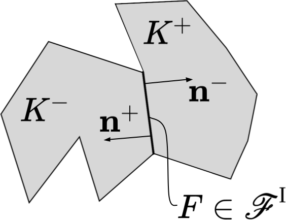
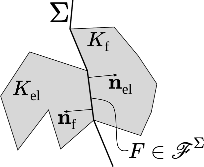
Figure 2: Polygonal elements sharing an internal face (left) or a face on the interface $\Sigma$ (right).

3.2 PolyDG semidiscrete problem

For a given integer $m\geq 1$, we introduce the following piecewise polynomial spaces:

$$X_{h}^{\text{DG}}(\Omega_{\star})=\{\phi\in L^{2}(\Omega_{\star})\colon\phi|_{K}\in\mathbb{P}^{m}(K)\quad\forall K\in\mathscr{T}_{\star}\},\qquad\star={\rm el},{\rm f}$$

$$Q^{\rm DG}_{{\rm j},h}=X_{h}^{\text{DG}}(\Omega_{\rm el}),\quad Q^{\rm DG}_{h}=X_{h}^{\text{DG}}(\Omega_{\rm f}),\quad{\bm{W}}^{\rm DG}_{h}=[X_{h}^{\text{DG}}(\Omega_{\rm el})]^{d},\quad{\bm{V}}^{\rm DG}_{h}=[X_{h}^{\text{DG}}(\Omega_{\rm f})]^{d}.$$

Moreover, we denote by $H^{s}(\mathscr{T}_{\rm el}),H^{s}(\mathscr{T}_{\rm f})$ the broken Sobolev spaces of order $s$ over the mesh of the poroelastic and fluid domains, namely $H^{s}(\mathscr{T}_{\star})=\{q\in L^{2}(\Omega_{\star})\colon q|_{K}\in H^{s}(K)\quad\forall K\in\mathscr{T}_{\star}\}$ for $\star={\rm el},{\rm f}$. We then introduce the following forms, for ${\bm{d}},{\bm{w}}\in[H^{1}(\mathscr{T}_{h,{\rm el}})]^{d},p_{\rm j},q_{\rm j}\in H^{1}(\mathscr{T}_{h,{\rm el}}),\text{ with }{\rm j}\in J,{\bm{u}},{\bm{v}}\in[H^{1}(\mathscr{T}_{h,{\rm f}})]^{d},p,q\in H^{1}(\mathscr{T}_{h,{\rm f}})$:

$$\begin{split}\mathcal{A}_{\rm el}({\bm{d}},{\bm{w}})&=\int_{\Omega_{\rm el}}\sigma_{\rm el}({\bm{d}})\colon\varepsilon_{h}({\bm{w}})\\ &\qquad-\sum_{F\in\mathscr{F}_{\rm el}^{\rm I}\cup\mathscr{F}_{\rm el}^{\rm D}}\int_{F}\left(\{\!\!\{\sigma_{\rm el}({\bm{d}})\}\!\!\}\colon[\![{\bm{w}}]\!]+[\![{\bm{d}}]\!]\colon\{\!\!\{\sigma_{\rm el}({\bm{w}})\}\!\!\}-\eta[\![{\bm{d}}]\!]\colon[\![{\bm{w}}]\!]\right),\end{split}$$ (7a)

$$\mathcal{F}_{\rm el}({\bm{w}}) =\int_{\Omega_{\rm el}}{\bm{f}}_{\rm el}\cdot{\bm{w}},$$ (7b)

$$\mathcal{B}_{\rm j}(p_{\rm j},{\bm{w}}) =-\int_{\Omega_{\rm el}}\alpha_{\rm j}p_{\rm j}\,{\rm div}_{h}\,{\bm{w}}+\sum_{F\in\mathscr{F}_{\rm el}^{\rm I}\cup\mathscr{F}_{\rm el}^{{\rm D}_{\rm j}}}\int_{F}\alpha_{\rm j}\{\!\!\{p_{\rm j}I\}\!\!\}\colon[\![{\bm{w}}]\!],,$$ (7c)

$$\begin{split}\mathcal{A}_{\rm j}(p_{\rm j},q_{\rm j})&=\int_{\Omega_{\rm el}}\mu_{\rm j}^{-1}K_{\rm j}\nabla_{h}p_{\rm j}\cdot\nabla_{h}q_{\rm j}\\ &-\sum_{F\in\mathscr{F}_{\rm el}^{\rm I}\cup\mathscr{F}_{\rm el}^{{\rm D}_{\rm j}}}\int_{F}\left(\{\!\!\{\mu_{\rm j}^{-1}K_{\rm j}\nabla_{h}p_{\rm j}\}\!\!\}\cdot[\![q_{\rm j}]\!]+[\![p_{\rm j}]\!]\cdot\{\!\!\{\mu_{\rm j}^{-1}K_{\rm j}\nabla_{h}q_{\rm j}\}\!\!\}-\zeta_{\rm j}[\![p_{\rm j}]\!]\cdot[\![q_{\rm j}]\!]\right),\end{split}$$ (7d)

$$\mathcal{C}_{\rm j}(\{p_{\rm k}\}_{{\rm k}\in J},q_{\rm j}) =\int_{\Omega_{\rm el}}\sum_{{\rm k}\in J}\beta_{{\rm k}{\rm j}}(p_{\rm j}-p_{\rm k})q_{\rm j}+\int_{\Omega_{\rm el}}\beta_{\rm j}^{\text{e}}p_{\rm j}q_{\rm j},$$ (7e)

$$\mathcal{F}_{\rm j}(q_{\rm j}) =\int_{\Omega_{\rm el}}g_{\rm j}q_{\rm j},$$ (7f)

$$\begin{split}\mathcal{A}_{\rm f}({\bm{u}},{\bm{v}})&=\int_{\Omega_{\rm f}}\sigma_{\rm f}({\bm{u}})\colon\varepsilon_{h}({\bm{v}})\\ &-\sum_{F\in\mathscr{F}_{\rm f}^{\rm I}\cup\mathscr{F}_{\rm f}^{\rm D}}\int_{F}\left(\{\!\!\{\sigma_{\rm f}({\bm{u}})\}\!\!\}\colon[\![{\bm{v}}]\!]+[\![{\bm{u}}]\!]\colon\{\!\!\{\sigma_{\rm f}({\bm{v}})\}\!\!\}-\gamma_{\bm{v}}[\![{\bm{u}}]\!]\colon[\![{\bm{v}}]\!]\right),\end{split}$$ (7g)

$$\mathcal{B}_{\rm f}(p,{\bm{v}}) =-\int_{\Omega_{\rm f}}p\,{\rm div}_{h}\,{\bm{v}}+\sum_{F\in\mathscr{F}_{\rm f}^{\rm I}\cup\mathscr{F}_{\rm f}^{{\rm D}}}\int_{F}\{\!\!\{pI\}\!\!\}\colon[\![{\bm{v}}]\!],$$ (7h)

$$\mathcal{F}_{\rm f}({\bm{v}}) =\int_{\Omega_{\rm f}}{\bm{f}}_{\rm f}\cdot{\bm{v}},$$ (7i)

$$\mathcal{S}(p,q) =\sum_{F\in\mathscr{F}_{\rm f}^{\rm I}}\int_{F}\gamma_{p}[\![p]\!]\cdot[\![q]\!],$$ (7j)

$$\mathcal{J}(p_{\rm E},{\bm{w}},{\bm{v}}) =\sum_{F\in\mathscr{F}^{\Sigma}}\int_{F}\left(\{\!\!\{p_{\rm E}I\}\!\!\}\colon[\![{\bm{w}},{\bm{v}}]\!]\right),$$ (7k)

where $\nabla_{h},\varepsilon_{h},{\rm div}_{h}$ denote the element-wise gradient, symmetric gradient, and divergence operators, respectively, and the stress tensors $\sigma_{\rm el},\sigma_{\rm f}$ are implicitly defined in terms of these piecewise operators. The parameters $\eta,\zeta_{\rm j},\gamma_{\bm{v}},\gamma_{p}$ appearing in these forms are defined as follows [14, 35]:

$$\eta=\overline{\eta}\frac{\overline{\mathbb{C}}_{\rm el}^{K}}{\{h\}_{\text{H}}},\qquad\zeta_{\rm j}=\overline{\zeta}_{\rm j}\frac{\overline{k}_{\rm j}^{K}}{\sqrt{\mu_{\rm j}}\{h\}_{\text{H}}},\qquad\gamma_{\bm{v}}=\overline{\gamma}_{\bm{v}}\frac{\mu}{\{h\}_{\text{H}}},\qquad\gamma_{p}=\overline{\gamma}_{p}\{h\}_{\text{H}},$$ (8)

where $\{h\}_{\text{H}}$ denotes the harmonic average on $K^{\pm}$ (with $\{h\}_{\text{H}}=h_{K}$ on Dirichlet faces) $\overline{\mathbb{C}}_{\rm el}^{K}=\|\mathbb{C}_{\rm el}^{1/2}|_{K}\|_{2}^{2},\overline{k}_{\rm j}^{K}=\|K_{\rm j}^{1/2}|_{K}\|_{2}^{2}$ are the $L^{2}$-norms of the symmetric second-order tensors appearing in the elasticity and Darcy equations, for each $K\in\mathscr{T}_{\rm el}$, and $\overline{\eta},\overline{\zeta_{\rm j}}\ \forall{\rm j}\in J,\overline{\gamma}_{\bm{v}},\overline{\gamma}_{p}$ are penalty constants to be chosen large enough.

The form $J(\cdot,\cdot,\cdot)$ is the piecewise discontinuous version of the interface form $\mathfrak{J}(\cdot,\cdot,\cdot)$ derived in Remark 2.1. Indeed, for any $p_{\rm E}\in H^{1}(\mathscr{T}_{h_{\rm el}}),{\bm{w}}\in[H^{1}(\mathscr{T}_{h,{\rm el}}]^{d},{\bm{v}}\in[H^{1}(\mathscr{T}_{h,{\rm f}})]^{d}$,

$$\mathfrak{J}(q_{\rm E},{\bm{w}},{\bm{v}}) =\sum_{F\in\mathscr{F}^{\Sigma}}\int_{F}\left[p_{\rm E}I\colon({\bm{w}}\odot{\bm{n}}_{\rm el}+{\bm{v}}\odot{\bm{n}}_{\rm f})-q_{\rm E}I\colon(\partial_{t}{\bm{d}}\odot{\bm{n}}_{\rm el}+{\bm{u}}\odot{\bm{n}}_{\rm f})\right]$$ (9)

$$=\sum_{F\in\mathscr{F}^{\Sigma}}\int_{F}\left[\{\!\!\{p_{\rm E}I\}\!\!\}\colon[\![{\bm{w}},{\bm{v}}]\!]-[\![\partial_{t}{\bm{d}},{\bm{u}}]\!]\colon\{\!\!\{q_{\rm E}I\}\!\!\}\right],$$

where we have used the identity ${\bm{a}}\cdot{\bm{b}}={{\bm{a}}\odot{\bm{b}}\ \colon I},\forall{\bm{a}},{\bm{b}}\in\mathbb{R}^{d}$ and then the definition of the average and jump operators introduced in Section 3.1.

Finally, the semidiscrete formulation reads as follows:
For any $t\in(0,T]$, find $({\bm{d}}_{h},\{p_{{\rm j},h}\}_{{\rm j}\in J},{\bm{u}}_{h},p_{h})\in{\bm{W}}^{\rm DG}_{h}\times\left(\bigtimes_{{\rm j}\in J}Q^{\rm DG}_{{\rm j},h}\right)\times{\bm{V}}^{\rm DG}_{h}\times Q^{\rm DG}_{h}$ such that

$$(\rho_{\rm el}\partial_{tt}^{2}{\bm{d}}_{h} ,{\bm{w}}_{h})_{\Omega_{\rm el}}+\mathcal{L}_{\rm el}({\bm{d}}_{h},\{p_{{\rm k},h}\}_{{\rm k}\in J};{\bm{w}}_{h})-\mathcal{F}_{\rm el}({\bm{w}}_{h})$$ (10)

$$+\sum_{{\rm j}\in J}\left[(c_{\rm j}\partial_{t}p_{{\rm j},h},q_{{\rm j},h})_{\Omega_{\rm el}}+\mathcal{L}_{\rm j}(\{p_{{\rm k},h}\}_{{\rm k}\in J},\partial_{t}{\bm{d}}_{h};q_{{\rm j},h})-\mathcal{F}_{\rm j}(q_{{\rm j},h})\right]$$

$$+(\rho_{\rm f}\partial_{t}{\bm{u}}_{h},{\bm{v}}_{h})_{\Omega_{\rm f}}+\mathcal{L}_{\rm f}({\bm{u}}_{h},p_{h};{\bm{v}}_{h},q_{h})-\mathcal{F}_{\rm f}({\bm{v}}_{h})$$

$$+\mathcal{J}(p_{{\rm E},h},{\bm{w}}_{h},{\bm{v}}_{h})-\mathcal{J}(q_{{\rm E},h},\partial_{t}{\bm{d}}_{h},{\bm{u}}_{h})=0$$

$$\forall{\bm{w}}_{h}\in{\bm{W}}^{\rm DG}_{h},{\bm{v}}_{h}\in{\bm{V}}^{\rm DG}_{h},q_{h}\in Q^{\rm DG}_{h},q_{{\rm j},h}\in Q^{\rm DG}_{{\rm j},h}.$$

Problem (10) is supplemented with suitable initial conditions ${\bm{d}}_{h}(0),\dot{{\bm{d}}}_{h}(0),\{p_{{\rm j},h}(0)\}_{{\rm j}\in J},{\bm{u}}_{h}(0)$ that are projections of the initial data introduced in (1e) onto the corresponding DG spaces. The bilinear forms appearing in (10) are defined as

$$\mathcal{L}_{\rm el}({\bm{d}},\{p_{\rm k}\}_{{\rm k}\in J};{\bm{w}}) =\mathcal{A}_{\rm el}({\bm{d}},{\bm{w}})+\sum_{{\rm k}\in J}\mathcal{B}_{\rm k}(p_{\rm k},{\bm{w}}),$$ (11a)

$$\mathcal{L}_{\rm j}(\{p_{\rm k}\}_{{\rm k}\in J},\partial_{t}{\bm{d}};q_{\rm j}) =\mathcal{A}_{\rm j}(p_{\rm j},q_{\rm j})+\mathcal{C}_{\rm j}(\{p_{\rm k}\}_{{\rm k}\in J},q_{\rm j})-\mathcal{B}_{\rm j}(q_{\rm j},\partial_{t}{\bm{d}}),\qquad\forall{\rm j}\in J,$$ (11b)

$$\mathcal{L}_{\rm f}({\bm{u}},p;{\bm{v}},q) =\mathcal{A}_{\rm f}({\bm{u}},{\bm{v}})+\mathcal{B}_{\rm f}(p,{\bm{v}})-\mathcal{B}_{\rm f}(q,{\bm{u}})+\mathcal{S}(p,q).$$ (11c)

3.3 Algebraic formulation

We introduce suitable sets of basis functions such that ${\rm span}\{\bm{\varphi}_{\rm el}^{i}\}_{i=0}^{N_{\rm el}}={\bm{W}}^{\rm DG}_{h}$, ${\rm span}\{\bm{\varphi}_{\rm el}^{i}\}_{i=0}^{N_{\rm f}}={\bm{V}}^{\rm DG}_{h}$, ${\rm span}\{\psi^{i}\}_{i=0}^{N_{p}}=Q^{\rm DG}_{h}$, ${\rm span}\{\psi_{\rm j}^{i}\}_{i=0}^{N_{\rm j}}=Q^{\rm DG}_{{\rm j},h}$ for ${\rm j}\in J$. Denoting by uppercase letters the d.o.f. vectors corresponding to the problem unknowns, the (formal) algebraic form of (10) is the following:
Given ${\bm{D}}_{0},\dot{{\bm{D}}}_{0},{\bm{U}}_{0},{\bm{P}}_{{\rm j}0},{\rm j}\in J$, find ${\bm{D}},{\bm{U}},{\bm{P}},{\bm{P}}_{\rm j},{\rm j}\in J$ such that

$$\begin{bmatrix}M_{\rm el}\partial_{tt}^{2}+A_{\rm el}&B_{\text{A}}^{T}&\cdots&B_{\text{E}}^{T}+J_{{\rm el}}^{T}&0&0\\ -B_{\text{A}}\partial_{t}&M_{\text{A}}\partial_{t}+A_{\text{A}}+C_{\text{A}\text{A}}&\cdots&C_{\text{A}\text{E}}&0&0\\ \vdots&\vdots&\vdots&\vdots&\vdots&\vdots\\ -B_{\rm E}+J_{{\rm el}}\partial_{t}&C_{{\rm E}\text{A}}&\cdots&M_{\rm E}\partial_{t}+A_{\rm E}+C_{{\rm E}{\rm E}}&-J_{{\rm f}}&0\\ 0&0&\cdots&J_{{\rm f}}^{T}&M_{\rm f}\partial_{t}+A_{\rm f}&B_{\rm f}^{T}\\ 0&0&\cdots&0&-B_{\rm f}&S\end{bmatrix}\begin{bmatrix}{\bm{D}}\\ {\bm{P}}_{\text{A}}\\ \vdots\\ {\bm{P}}_{\rm E}\\ {\bm{U}}\\ {\bm{P}}\end{bmatrix}=\begin{bmatrix}{\bm{F}}_{\rm el}\\ {\bm{F}}_{\text{A}}\\ \vdots\\ {\bm{F}}_{\rm E}\\ {\bm{F}}_{\rm f}\\ {\bm{0}}\end{bmatrix}$$ (12)

The matrices and vectors of (12) are defined as follows (where $\star={\rm el},{\rm f}$):

$$[M_{\star}]_{ij} =(\rho_{\star}\bm{\varphi}_{\star}^{j},\bm{\varphi}_{\star}^{i})_{\Omega_{\star}}, [M_{\rm j}]_{ij} =(c_{\rm j}\psi_{\rm j}^{j},\phi_{\rm j}^{i})_{\Omega_{\rm el}}, [S]_{ij} =\mathcal{S}(\psi^{j},\phi^{i})$$

$$[A_{\star}]_{ij} =\mathcal{A}_{\star}(\bm{\varphi}_{\star}^{j},\bm{\varphi}_{\star}^{i}), [A_{\rm j}]_{ij} =\mathcal{A}_{\rm j}(\psi_{\rm j}^{j},\phi_{\rm j}^{i}), [C_{\rm j}]_{ij} =\mathcal{C}_{\rm j}(\{\psi_{\rm k}^{i}\}_{{\rm k}\in J},\psi_{\rm j}^{i}),$$

$$[B_{\rm f}]_{ij} =\mathcal{B}_{\rm f}(\psi^{i},\bm{\varphi}_{\rm f}^{j}), [B_{\rm j}]_{ij} =\mathcal{B}_{\rm j}(\psi_{\rm j}^{i},\varphi_{\rm el}^{i}), [J_{\star}]_{ij} =\sum_{F\in\mathscr{F}^{\Sigma}}\int_{F}\{\!\!\{q_{\text{E}}^{j}I\}\!\!\}\colon\bm{\varphi}_{\star}^{i}\odot{\bm{n}}_{\star},$$

$$[F_{\star}]_{i} =\mathcal{F}_{\star}({\bm{\varphi}}_{\star}^{i}), [F_{\rm j}]_{i} =\mathcal{F}_{\rm j}(\psi_{\rm j}^{i}).$$

4 A priori analysis of the semidiscrete problem

For the analysis contained in this section, we consider a generic set $J$ of $N_{J}\in\mathbb{N}_{0}$ compartments and we assume that all the physical parameters of the model (defined in Table 1) are piecewise constant. For $r\geq 1$, we introduce the following broken norms [35, 14]:

$$|\mkern-1.5mu|{\bm{d}}|\mkern-1.5mu|_{{\rm DG},{\rm D}}^{2} =\|{\mathbb{C}_{\rm el}^{1}{2}}[\varepsilon_{h}({\bm{d}})]\|_{L^{2}(\mathscr{T}_{\rm el})}^{2}+\|\sqrt{\eta}[\![{\bm{d}}]\!]\|_{\mathscr{F}_{{\rm el},h}^{{\rm I}}\cup\mathscr{F}_{{\rm el},h}^{{\rm D}}}^{2} \forall{\bm{d}}\in{\bm{H}}^{r}(\mathscr{T}_{h}),$$ (13a)

$$|\mkern-1.5mu|p|\mkern-1.5mu|_{{\rm DG},{\rm P}_{\rm j}}^{2} =\|\mu_{\rm j}^{-1/2}K_{\rm j}^{1/2}\nabla_{h}p\|_{L^{2}(\mathscr{T}_{\rm el})}^{2}+\|\sqrt{\zeta_{\rm j}}[\![p]\!]\|^{2}_{\mathscr{F}_{{\rm el},h}^{{\rm I}}\cup\mathscr{F}_{{\rm el},h}^{{\rm D}_{\rm j}}} \forall p\in H^{r}(\mathscr{T}_{h}),$$ (13b)

$$|\mkern-1.5mu|{\bm{u}}|\mkern-1.5mu|_{{\rm DG},{\rm U}}^{2} =\|\sqrt{2\mu}\,\varepsilon_{h}({\bm{u}})\|_{L^{2}(\mathscr{T}_{\rm f})}^{2}+\|\sqrt{\gamma_{\bm{v}}}[\![{\bm{u}}]\!]\|^{2}_{\mathscr{F}_{{\rm f},h}^{{\rm I}}} \forall{\bm{u}}\in{\bm{H}}^{r}(\mathscr{T}_{h}),$$ (13c)

$$|\mkern-1.5mu|q|\mkern-1.5mu|_{{\rm DG},{\rm P}_{\rm f}}^{2} =\|q\|_{L^{2}(\Omega_{\rm f})}^{2}+\|\sqrt{\gamma_{p}}[\![q]\!]\|^{2}_{\mathscr{F}_{{\rm f},h}^{{\rm I}}\cup\mathscr{F}_{{\rm f},h}^{{\rm D}}} \forall q\in H^{r}(\mathscr{T}_{h}).$$ (13d)

We introduce the energy norms at time $t\in(0,T]$

$$|\mkern-1.5mu|({\bm{d}},\{p_{\rm j}\}_{{\rm j}\in J})|\mkern-1.5mu|_{{\rm el},t} =\left[\|\sqrt{\rho_{\rm el}}\partial_{t}{\bm{d}}(t)\|_{\Omega_{\rm el}}^{2}+|\mkern-1.5mu|{\bm{d}}(t)|\mkern-1.5mu|_{{\rm DG},{\rm D}}^{2}\phantom{\sum_{{\rm j}\in J}\int_{0}^{t}}\right.$$

$$\qquad\left.+\sum_{{\rm j}\in J}\left(\|\sqrt{c_{\rm j}}p_{\rm j}(t)\|_{\Omega_{\rm el}}^{2}+\int_{0}^{t}\left(|\mkern-1.5mu|p_{\rm j}(s)|\mkern-1.5mu|_{{\rm DG},{\rm P}_{\rm j}}^{2}+\|\sqrt{\beta^{\text{e}}_{\rm j}}p_{\rm j}(s)\|_{\Omega_{\rm el}}^{2}\right)ds\right)\right]^{1/2},$$

$$|\mkern-1.5mu|({\bm{u}},p)|\mkern-1.5mu|_{{\rm f},t} =\left[\|\sqrt{\rho_{\rm f}}{\bm{u}}(t)\|_{\Omega_{\rm f}}^{2}+\int_{0}^{t}\left(|\mkern-1.5mu|{\bm{u}}(s)|\mkern-1.5mu|_{{\rm DG},{\rm U}}^{2}+|\mkern-1.5mu|p(s)|\mkern-1.5mu|_{{\rm DG},{\rm P}_{\rm f}}^{2}\right)ds\right]^{1/2},$$

and set

$$|\mkern-1.5mu|({\bm{d}},\{p_{\rm j}\}_{{\rm j}\in J},{\bm{u}},p)|\mkern-1.5mu|_{{\rm EN},t} =\left[|\mkern-1.5mu|({\bm{d}},\{p_{\rm j}\}_{{\rm j}\in J})|\mkern-1.5mu|_{{\rm el},t}^{2}+|\mkern-1.5mu|({\bm{u}},p)|\mkern-1.5mu|_{{\rm f},t}^{2}\right]^{1/2}.$$ (14)

For the sake of simplicity, in the inequalities appearing in the following analysis, we neglect the dependencies on the model parameters and the polynomial degree $m$, and we use the notation $x\lesssim y$ to indicate that $\exists C>0:x\leq Cy$, where $C$ is independent of the mesh discretization parameters. Moreover, we make the following assumption on the mesh [11, 30]:

Assumption 4.1

For each $h>0$, the two meshes $\mathscr{T}_{h,{\rm el}},\mathscr{T}_{h,{\rm f}}$ are aligned with $\Sigma$, namely there is no gap nor overlap between them (hanging nodes are allowed). Moreover, denoting by $\mathscr{T}_{h}$ the union of $\mathscr{T}_{h,{\rm el}}$ and $\mathscr{T}_{h,{\rm f}}$, we consider a sequence of meshes $\{\mathscr{T}_{h}\}_{h>0}$ satisfying the regularity requirements of [35]:

• $\{\mathscr{T}_{h}\}_{h>0}$ is $h$-uniformly polytopic-regular, namely for each $K\in\mathscr{T}_{h}$ there exists a set $\{S_{K}^{F}\}_{F\subset\partial K}$ of non-overlapping $d$-dimensional simplices contained in $\overline{K}$ such that

  $$\forall F\subset\partial K\colon\overline{F}=\overline{\partial K}\cap\overline{S_{K}^{F}}\text{ it holds that }h_{K}\lesssim d|S_{K}^{F}||F|^{-1},$$

  where $h_{K}$ is the diameter of $K$, and the cardinality of $\{S_{K}^{F}\}_{F\subset\partial K}$ does not depend on $h>0$.

• There exists a shape-regular simplicial covering $\widehat{\mathscr{T}}_{h}$ of $\mathscr{T}_{h}$ such that, for each $K\in\mathscr{T}_{h},\widehat{K}\in\widehat{\mathscr{T}}_{h}$ with $\widehat{K}\subseteq K$,

  $$h_{K}\lesssim h_{\widehat{K}},\max_{K\in\mathscr{T}_{h}}{\rm card}\{K^{\prime}\in\mathscr{T}_{h}\colon\exists\widehat{K}\in\widehat{\mathscr{T}}_{h}\text{ such that }K\subset\widehat{K}\text{ and }K^{\prime}\cap\widehat{K}\neq\emptyset\}\lesssim 1.$$

• The mesh size satisfies a local bounded variation property:

  $$\forall K_{1},K_{2}\in\mathscr{T}_{h}\colon|\partial K_{1}\cap\partial K_{2}|_{d-1}>0\qquad h_{K_{1}}\lesssim h_{K_{2}}\lesssim h_{K_{1}},$$

  with $|\cdot|_{d-1}$ denotes the $(d-1)$-dimensional measure and all the hidden constants independent of $h$ and the number of faces of $K_{1}$ and $K_{2}$.

Under these assumptions, we can prove the following stability result:

Theorem 4.1 (Stability estimate)

Let Assumption 4.1 hold true and let us also assume that the penalty constants defined in (8) are chosen sufficiently large. Then, the semidiscrete solution $({\bm{d}}_{h},\{p_{{\rm j},h}\}_{{\rm j}\in J},{\bm{u}}_{h},p_{h})$ of (10) satisfies the following inequality for each $t\in(0,T]$:

$$|\mkern-1.5mu|({\bm{d}}_{h},\{p_{{\rm j},h}\}_{{\rm j}\in J},{\bm{u}}_{h},p_{h})|\mkern-1.5mu|_{{\rm EN},t}\lesssim |\mkern-1.5mu|({\bm{d}}_{h},\{p_{{\rm j},h}\}_{{\rm j}\in J},{\bm{u}}_{h},0)|\mkern-1.5mu|_{{\rm EN},0}$$ (15)

$$+\int_{0}^{t}\left(\frac{1}{\sqrt{\rho_{\rm el}}}\|{\bm{f}}_{\rm el}\|_{\Omega_{\rm el}}+\sum_{{\rm j}\in J}\frac{1}{\sqrt{c_{\rm j}}}\|g_{\rm j}\|_{\Omega_{\rm el}}+\frac{1}{\sqrt{\rho_{\rm f}}}\|{\bm{f}}_{\rm f}\|_{\Omega_{\rm f}}\right)ds,$$

where, according to the initial conditions of (1e),

$$|\mkern-1.5mu|({\bm{d}}_{h},\{p_{{\rm j},h}\}_{{\rm j}\in J},{\bm{u}}_{h},0)|\mkern-1.5mu|_{{\rm EN},0}=\left[\|\sqrt{\rho_{\rm el}}\dot{{\bm{d}}}_{h}^{0}\|_{\Omega_{\rm el}}^{2}+|\mkern-1.5mu|{\bm{d}}_{h}^{0}|\mkern-1.5mu|_{{\rm DG},{\rm D}}^{2}+\sum_{{\rm j}\in J}\|\sqrt{c_{\rm j}}p_{{\rm j},h}^{0}\|_{\Omega_{\rm el}}^{2}+\|\sqrt{\rho_{\rm f}}{\bm{u}}_{h}^{0}\|_{\Omega_{\rm f}}^{2}\right]^{1/2}.$$

Proof.  Let us fix a time $t\in(0,T]$ and consider the following test functions in (6): ${\bm{w}}=\partial_{t}{\bm{d}}(t),{\bm{v}}={\bm{u}}(t),q=p(t),q_{\rm j}=p_{\rm j}(t)\ \forall{\rm j}\in J$. With this choice of test functions, the terms $\mathcal{J}$ cancel out, as well as the $\mathcal{B}$ forms in the $\mathcal{L}$ terms . Therefore, (6) becomes

$$(\rho_{\rm el}\partial_{tt}^{2} {\bm{d}}(t),\partial_{t}{\bm{d}}(t))_{\Omega_{\rm el}}+\mathcal{A}_{\rm el}({\bm{d}}(t),\partial_{t}{\bm{d}}(t))$$ (16)

$$\quad+\sum_{{\rm j}\in J}\left[(c_{\rm j}\partial_{t}p_{\rm j}(t),p_{\rm j}(t))_{\Omega_{\rm el}}+\mathcal{A}_{\rm j}(p_{\rm j}(t),p_{\rm j}(t))+\mathcal{C}_{\rm j}(\{p_{\rm k}(t)\}_{{\rm k}\in J},p_{\rm j}(t))\right]$$

$$\quad+(\rho_{\rm f}\partial_{t}{\bm{u}}(t),{\bm{u}}(t))_{\Omega_{\rm f}}+\mathcal{L}_{\rm f}({\bm{u}}(t),p(t);{\bm{u}}(t),p(t))$$

$$=\mathcal{F}_{\rm el}(\partial_{t}{\bm{d}}(t))+\sum_{{\rm j}\in J}\mathcal{F}_{\rm j}(p_{\rm j}(t))+\mathcal{F}_{\rm f}({\bm{u}}(t)).$$

Proceeding as in [35], we integrate (16) w.r.t. time and we can employ integration by parts in time in the following terms to obtain

$$\int_{0}^{t}(\rho_{\rm el}\partial_{tt}^{2}{\bm{d}}(s),\partial_{t}{\bm{d}}(s))_{\Omega_{\rm el}}ds =\frac{1}{2}\|\sqrt{\rho_{\rm el}}\partial_{t}{\bm{d}}(t)\|_{\Omega_{\rm el}}^{2}-\frac{1}{2}\|\sqrt{\rho_{\rm el}}\dot{{\bm{d}}}^{0}\|_{\Omega_{\rm el}}^{2},$$

$$\int_{0}^{t}\mathcal{A}_{\rm el}({\bm{d}}(s),\partial_{t}{\bm{d}}(s))ds =\frac{1}{2}\mathcal{A}_{\rm el}({\bm{d}}(t),{\bm{d}}(t))-\frac{1}{2}\mathcal{A}_{\rm el}({\bm{d}}^{0},{\bm{d}}^{0})$$

$$\int_{0}^{t}(c_{\rm j}\partial_{t}p_{\rm j}(s),p_{\rm j}(s))_{\Omega_{\rm el}}ds =\frac{1}{2}\|\sqrt{c_{\rm j}}p_{\rm j}(t)\|_{\Omega_{\rm el}}^{2}-\frac{1}{2}\|\sqrt{c_{\rm j}}p_{\rm j}^{0}\|_{\Omega_{\rm el}}^{2},\qquad\forall{\rm j}\in J,$$

$$\int_{0}^{t}(\rho_{\rm f}\partial_{t}{\bm{u}}(s),{\bm{u}}(s))_{\Omega_{\rm f}}ds =\frac{1}{2}\|\sqrt{\rho_{\rm f}}{\bm{u}}(t)\|_{\Omega_{\rm f}}^{2}-\frac{1}{2}\|\sqrt{\rho_{\rm f}}{\bm{u}}^{0}\|_{\Omega_{\rm f}}^{2}.$$

Using these identities and the definition of the bulk and broken norms introduced above, we can rewrite the left-hand side of (16) (integrated over time) as follows, and use Cauchy-Schwarz’s and Young’s inequalities on the right-hand side:

$$\| \sqrt{\rho_{\rm el}}\partial_{t}{\bm{d}}(t)\|_{\Omega_{\rm el}}^{2}\|\sqrt{\rho_{\rm el}}\dot{{\bm{d}}}^{0}\|_{\Omega_{\rm el}}^{2}+\mathcal{A}_{\rm el}({\bm{d}}(t),{\bm{d}}(t))-\mathcal{A}_{\rm el}({\bm{d}}^{0},{\bm{d}}^{0})$$ (17)

$$\quad+\sum_{{\rm j}\in J}\left[\|\sqrt{c_{\rm j}}p_{\rm j}(t)\|_{\Omega_{\rm el}}^{2}-\|\sqrt{c_{\rm j}}p_{\rm j}^{0}\|_{\Omega_{\rm el}}^{2}+2\int_{0}^{t}\left(\mathcal{A}_{\rm j}(p_{\rm j}(s),p_{\rm j}(s))+\mathcal{C}_{\rm j}(\{p_{\rm k}(s)\}_{{\rm k}\in J},p_{\rm j}(s))\right)ds\right]$$

$$\quad+\|\sqrt{\rho_{\rm f}}{\bm{u}}(t)\|_{\Omega_{\rm f}}^{2}-\|\sqrt{\rho_{\rm f}}{\bm{u}}^{0}\|_{\Omega_{\rm f}}^{2}+2\int_{0}^{t}\mathcal{L}_{\rm f}({\bm{u}}(s),p(s);{\bm{u}}(s),p(s))ds$$

$$\leq\int_{0}^{t}\left(\left\|\frac{1}{\sqrt{\rho_{\rm el}}}{\bm{f}}_{\rm el}(s)\right\|_{\Omega_{\rm el}}^{2}+\|\sqrt{\rho_{\rm el}}\partial_{t}{\bm{d}}(s)\|_{\Omega_{\rm el}}^{2}+\sum_{{\rm j}\in J}\left\|\frac{1}{\sqrt{c_{\rm j}}}g_{\rm j}(s)\right\|_{\Omega_{\rm el}}^{2}\right.$$

$$\left.\qquad\qquad+\sum_{{\rm j}\in J}\|\sqrt{c_{\rm j}}p_{\rm j}(s)\|_{\Omega_{\rm el}}^{2}+\left\|\frac{1}{\sqrt{\rho_{\rm f}}}{\bm{f}}_{\rm f}(s)\right\|_{\Omega_{\rm f}}^{2}+\|\sqrt{\rho_{\rm f}}{\bm{u}}(s)\|_{\Omega_{\rm f}}^{2}\right)ds.$$

We now consider continuity and coercivity results for the bilinear forms appearing in (17) with respect to the broken norms (13). These results, proven in [35, 14], are reported in Appendix A (Lemma A.1) and they include an inf-sup condition for the form $\mathcal{B}_{\rm f}$, with a constant $\beta_{{\rm f},h}$ independent of the mesh elements size. According to [14], if $\gamma_{\bm{v}}$ is large enough, there exists $\alpha>0$ such that $\alpha=\mathcal{O}(\beta_{{\rm f},h}^{-2})$ and

$$\mathcal{L}_{\rm f}({\bm{u}}(s),p(s);{\bm{u}}(s),p(s))\geq\alpha(|\mkern-1.5mu|{\bm{u}}(s)|\mkern-1.5mu|_{{\rm DG},{\rm U}}^{2}+|\mkern-1.5mu|p(s)|\mkern-1.5mu|_{{\rm DG},{\rm P}_{\rm f}}^{2}).$$

Analogously, the coercivity results of the forms $\mathcal{A}_{\rm el},\mathcal{A}_{\rm j},\mathcal{C}_{\rm j}$ and the continuity of $\mathcal{A}_{\rm el}$ yield [35]

$$\mathcal{A}_{\rm el}({\bm{d}}(t), {\bm{d}}(t))-\mathcal{A}_{\rm el}({\bm{d}}^{0},{\bm{d}}^{0})+2\sum_{{\rm j}\in J}\int_{0}^{t}\left(\mathcal{A}_{\rm j}(p_{\rm j}(s),p_{\rm j}(s))+\mathcal{C}_{\rm j}(\{p_{\rm k}(s)\}_{{\rm k}\in J},p_{\rm j}(s))\right)ds$$

$$\gtrsim|\mkern-1.5mu|{\bm{d}}(t)|\mkern-1.5mu|_{{\rm DG},{\rm D}}^{2}-|\mkern-1.5mu|{\bm{d}}^{0}|\mkern-1.5mu|_{{\rm DG},{\rm D}}^{2}+\sum_{{\rm j}\in J}\int_{0}^{t}\left(|\mkern-1.5mu|p_{\rm j}(s)|\mkern-1.5mu|_{{\rm DG},{\rm P}_{\rm j}}^{2}+\|\sqrt{\beta_{\rm j}^{\text{e}}}p_{\rm j}(s)\|_{\Omega_{\rm el}}^{2}\right)ds.$$

We can use these results on the left-hand side of (17) to obtain

$$\|\sqrt{\rho_{\rm el}}\partial_{t}{\bm{d}}(t)\|_{\Omega_{\rm el}}^{2} +|\mkern-1.5mu|{\bm{d}}(t)|\mkern-1.5mu|_{{\rm DG},{\rm D}}^{2}+\sum_{{\rm j}\in J}\left[\|\sqrt{c_{\rm j}}p_{\rm j}(t)\|_{\Omega_{\rm el}}^{2}+\int_{0}^{t}\left(|\mkern-1.5mu|p_{\rm j}(s)|\mkern-1.5mu|_{{\rm DG},{\rm P}_{\rm j}}^{2}+\|\sqrt{\beta^{\text{e}}_{\rm j}}p_{\rm j}(s)\|_{\Omega_{\rm el}}^{2}\right)ds\right]$$

$$\qquad-\|\sqrt{\rho_{\rm el}}\dot{{\bm{d}}}^{0}\|_{\Omega_{\rm el}}^{2}-|\mkern-1.5mu|{\bm{d}}^{0}|\mkern-1.5mu|_{{\rm DG},{\rm D}}^{2}-\sum_{{\rm j}\in J}\|\sqrt{c_{\rm j}}p_{\rm j}^{0}\|_{\Omega_{\rm el}}^{2}$$

$$\qquad+|\mkern-1.5mu|({\bm{u}}(t),p(t))|\mkern-1.5mu|_{{\rm f},t}^{2}-\|\sqrt{\rho_{\rm f}}{\bm{u}}^{0}\|_{\Omega_{\rm f}}^{2}$$

$$\lesssim\int_{0}^{t}\left(\left\|\frac{1}{\sqrt{\rho_{\rm el}}}{\bm{f}}_{\rm el}(s)\right\|_{\Omega_{\rm el}}^{2}+\sum_{{\rm j}\in J}\left\|\frac{1}{\sqrt{c_{\rm j}}}g_{\rm j}(s)\right\|_{\Omega_{\rm el}}^{2}+\left\|\frac{1}{\sqrt{\rho_{\rm f}}}{\bm{f}}_{\rm f}(s)\right\|_{\Omega_{\rm f}}^{2}\right)ds.$$

The definitions of $|\mkern-1.5mu|\cdot|\mkern-1.5mu|_{{\rm EN},t}$ and $|\mkern-1.5mu|\cdot|\mkern-1.5mu|_{{\rm EN},0}$ and the fact that $\rho_{\rm el},c_{\rm j},\rho_{\rm f}$ are constant conclude the proof.

We now proceed to derive an a-priori error estimate for the error introduced by the space discretization of the problem. For any $t\in(0,T]$, let $({\bm{d}},\{p_{\rm j}\}_{{\rm j}\in J},{\bm{u}},p)$ denote the weak solution of problem (6) and let $({\bm{d}}_{h},\{p_{{\rm j},h}\}_{{\rm j}\in J},{\bm{u}}_{h},p_{h})$ denote the semidiscrete solution of problem (10), obtained with sufficiently large stability parameters as defined in (8).

Using the inverse trace inequality [13, 11]

$$\|\phi\|_{\partial K}^{2}\lesssim h_{K}^{-1}\|\phi\|_{K}^{2}\qquad\forall\phi\in\mathbb{P}^{m}(K),K\in\mathscr{T}_{h},$$ (18)

we can state the following continuity result for the interface forms, whose proof is provided in Appendix B:

Lemma 4.1

Under Assumption 4.1, the following inequalities hold:

$$|\mathcal{J}(q,{\bm{w}}_{h},{\bm{v}}_{h})| \lesssim\|\eta^{1/2}q\|_{\mathscr{F}_{h}^{\Sigma}}|\mkern-1.5mu|{\bm{w}}_{h}|\mkern-1.5mu|_{{\rm DG},{\rm D}}+\|\gamma_{p}^{-1/2}q\|_{\mathscr{F}_{h}^{\Sigma}}|\mkern-1.5mu|{\bm{v}}_{h}|\mkern-1.5mu|_{{\rm DG},{\rm U}}$$

$$\qquad\qquad\forall q\in H^{2}(\mathscr{T}_{h,{\rm el}}),{\bm{w}}_{h}\in{\bm{W}}^{\rm DG}_{h},{\bm{v}}_{h}\in{\bm{V}}^{\rm DG}_{h},$$

$$|\mathcal{J}(q_{h},{\bm{w}},{\bm{v}})| \lesssim|\mkern-1.5mu|q_{h}|\mkern-1.5mu|_{{\rm DG},{\rm P}_{\rm f}}\|\eta^{1/2}{\bm{w}}\|_{\mathscr{F}_{h}^{\Sigma}}+|\mkern-1.5mu|q_{h}|\mkern-1.5mu|_{{\rm DG},{\rm P}_{\rm f}}\|\gamma_{\bm{v}}^{1/2}{\bm{v}}\|_{\mathscr{F}_{h}^{\Sigma}}$$

$$\qquad\qquad\forall q_{h}\in Q^{\rm DG}_{{\rm E},h},{\bm{w}}\in[H^{2}(\mathscr{T}_{h,{\rm f}})]^{d},{\bm{v}}\in[H^{2}(\mathscr{T}_{h,{\rm f}})]^{d}.$$

We introduce the following additional norms for non-discrete functions:

$$\begin{aligned} |\mkern-1.5mu|\mkern-1.5mu|{\bm{w}}|\mkern-1.5mu|\mkern-1.5mu|_{{\rm D}}^{2}&=|\mkern-1.5mu|{\bm{w}}|\mkern-1.5mu|_{{\rm DG},{\rm D}}^{2}+\|\eta^{-1/2}\{\!\!\{\sigma_{\rm el}({\bm{w}})\}\!\!\}\|_{\mathscr{F}_{{\rm el},h}^{\text{I}}\cup\mathscr{F}_{{\rm el},h}^{\text{D}}}^{2}&\qquad\forall{\bm{w}}\in[H^{2}(\mathscr{T}_{h,{\rm el}})]^{d},\\ |\mkern-1.5mu|\mkern-1.5mu|q_{\rm j}|\mkern-1.5mu|\mkern-1.5mu|_{{\rm P}_{\rm j}}^{2}&=|\mkern-1.5mu|q_{\rm j}|\mkern-1.5mu|_{{\rm DG},{\rm P}_{\rm j}}^{2}+\|\zeta^{-1/2}\{\!\!\{\frac{1}{\mu_{\rm j}}K_{\rm j}\nabla_{h}q_{\rm j}\}\!\!\}\|_{\mathscr{F}_{{\rm el},h}^{\text{I}}\cup\mathscr{F}_{{\rm el},h}^{\text{D}_{\rm j}}}^{2}&\qquad\forall q_{\rm j}\in H^{2}(\mathscr{T}_{h,{\rm el}}),\qquad\forall{\rm j}\in J,\\ |\mkern-1.5mu|\mkern-1.5mu|{\bm{v}}|\mkern-1.5mu|\mkern-1.5mu|_{{\rm U}}^{2}&=|\mkern-1.5mu|{\bm{v}}|\mkern-1.5mu|_{{\rm DG},{\rm U}}^{2}+\|\gamma_{{\bm{v}}}^{-1/2}\{\!\!\{\sigma_{\rm f}({\bm{v}})\}\!\!\}\|_{\mathscr{F}_{{\rm f},h}^{\text{I}}\cup\mathscr{F}_{{\rm f},h}^{\text{D}}}^{2}&\qquad\forall{\bm{v}}\in[H^{2}(\mathscr{T}_{h,{\rm f}})]^{d},\\ |\mkern-1.5mu|\mkern-1.5mu|q|\mkern-1.5mu|\mkern-1.5mu|_{{\rm P}_{\rm f}}^{2}&=|\mkern-1.5mu|q|\mkern-1.5mu|_{{\rm DG},{\rm P}_{\rm f}}^{2}+\|{\gamma_{p}^{1/2}}\{\!\!\{q\}\!\!\}\|_{\mathscr{F}_{{\rm f},h}^{\text{I}}}^{2}&\qquad\forall q\in H^{1}(\mathscr{T}_{h,{\rm f}}),\end{aligned}$$

$$|\mkern-1.5mu|\mkern-1.5mu|({\bm{w}},\{q_{\rm j}\}_{{\rm j}\in J},{\bm{v}},p)|\mkern-1.5mu|\mkern-1.5mu|^{2}=|\mkern-1.5mu|\mkern-1.5mu|{\bm{w}}|\mkern-1.5mu|\mkern-1.5mu|_{{\rm D}}^{2}+\sum_{{\rm j}\in J}|\mkern-1.5mu|\mkern-1.5mu|q_{\rm j}|\mkern-1.5mu|\mkern-1.5mu|_{{\rm P}_{\rm j}}^{2}+|\mkern-1.5mu|\mkern-1.5mu|{\bm{v}}|\mkern-1.5mu|\mkern-1.5mu|_{{\rm U}}^{2}+|\mkern-1.5mu|\mkern-1.5mu|q|\mkern-1.5mu|\mkern-1.5mu|_{{\rm P}_{\rm f}}^{2}.$$

Denoting by $\mathscr{E}_{K}:H^{s}(\Omega)\to H^{s}(\mathbb{R}^{d})$ the Stein extension operator for a Lipschitz domain $\Omega$ defined in [69], the following interpolation result can be stated (cf. [35, 14, 8, 6]):

Lemma 4.2

Under Assumption 4.1, the following estimates hold:

$$\forall({\bm{w}},\{q_{\rm j}\}_{{\rm j}\in J},{\bm{v}},q)\in[H^{m+1}(\mathscr{T}_{h,{\rm el}})]^{d+N_{J}}\times[H^{m+1}(\mathscr{T}_{h,{\rm f}})]^{d+1}$$

$$\exists({\bm{w}}_{I},\{q_{{\rm j}I}\}_{{\rm j}\in J},{\bm{v}}_{I},q_{I})\in{\bm{W}}^{\rm DG}_{h}\times\bigtimes_{{\rm j}\in J}Q^{\rm DG}_{{\rm j},h}\times{\bm{V}}^{\rm DG}_{h}\times Q^{\rm DG}_{h}\quad\text{such that}$$

$$i)\ |\mkern-1.5mu|\mkern-1.5mu|({\bm{w}}-{\bm{w}}_{I},\{q_{\rm j}-q_{{\rm j}I}\}_{{\rm j}\in J},{\bm{v}}-{\bm{v}}_{I},q-q_{I})|\mkern-1.5mu|\mkern-1.5mu|^{2}$$

$$\qquad\lesssim\sum_{K\in\mathscr{T}_{h,{\rm el}}}h_{K}^{2m}\left(\|\mathcal{E}_{K}{\bm{w}}\|_{[H^{m+1}(\widehat{K})]^{d}}^{2}+\sum_{{\rm j}\in J}\|\mathcal{E}_{\rm j}q_{\rm j}\|_{H^{m+1}(\widehat{K})}^{2}+\|\mathcal{E}_{K}{\bm{d}}\|_{[H^{m+1}(\widehat{K})]^{d}}^{2}+\|\mathcal{E}_{K}p\|_{H^{m+1}(\widehat{K})}^{2}\right),$$

$$ii)\ \|{\bm{w}}\|_{\mathscr{F}^{\Sigma}}^{2}+\sum_{{\rm j}\in J}\|q_{\rm j}\|_{\mathscr{F}^{\Sigma}}^{2}+\|{\bm{v}}\|_{\mathscr{F}^{\Sigma}}^{2}+\|q\|_{\mathscr{F}^{\Sigma}}^{2}$$

$$\qquad\lesssim\sum_{K\in\mathscr{T}_{h,{\rm el}}}h_{K}^{2m+1}\left(\|\mathcal{E}_{K}{\bm{w}}\|_{[H^{m+1}(\widehat{K})]^{d}}^{2}+\sum_{{\rm j}\in J}\|\mathcal{E}_{\rm j}q_{\rm j}\|_{H^{m+1}(\widehat{K})}^{2}+\|\mathcal{E}_{K}{\bm{d}}\|_{[H^{m+1}(\widehat{K})]^{d}}^{2}+\|\mathcal{E}_{K}p\|_{H^{m+1}(\widehat{K})}^{2}\right),$$

where $\widehat{K}\supseteq K$, for each $K\in\mathscr{T}_{h}$, are shape-regular simplexes as in Assumption 4.1.

Combining the results above, we can prove the following optimal convergence result, whose proof is provided in Appendix C.

Theorem 4.2 (A priori error estimate)

Under the same assumptions of Theorem 4.1, if the solution of problem (6) is sufficiently regular, and the initial conditions ${\bm{d}}^{0},\dot{{\bm{d}}}^{0},{\bm{u}}^{0},p_{\rm j}^{0},{\rm j}\in J$ are sufficiently regular, the following estimate holds for each $t\in(0,T]$ and for each $m\geq 1$:

$$|\mkern-1.5mu|({\bm{e}}^{\bm{d}},\{e^{P_{\rm j}}\}_{{\rm j}\in J},{\bm{e}}^{\bm{u}},e^{P_{\rm f}})|\mkern-1.5mu|_{{\rm EN},t}^{2}$$ (19)

$$\qquad\lesssim\sum_{K\in\mathscr{T}_{h,{\rm el}}}{h_{K}^{2m}}\left\{\|\mathcal{E}_{K}{\bm{d}}(t)\|_{[H^{m+1}(\widehat{K})]^{d}}^{2}+\sum_{{\rm k}\in J}\|\mathcal{E}_{K}p_{\rm k}(t)\|_{H^{m+1}(\widehat{K})}^{2}\right.$$

$$\qquad\qquad\qquad\left.+\int_{0}^{t}\left[\|\mathcal{E}_{K}\partial_{t}{\bm{d}}(s)\|_{[H^{m+1}(\widehat{K})]^{d}}^{2}+\|\mathcal{E}_{K}\partial_{tt}^{2}{\bm{d}}(s)\|_{[H^{m+1}(\widehat{K})]^{d}}^{2}\right]ds\right.$$

$$\qquad\qquad\qquad\left.+\int_{0}^{t}\left.\sum_{{\rm k}\in J}\left(\|\mathcal{E}_{K}p_{\rm k}(s)\|_{H^{m+1}(\widehat{K})}^{2}+\|\mathcal{E}_{K}\partial_{t}p_{\rm k}(s)\|_{H^{m+1}(\widehat{K})}^{2}\right)\right.ds\right\}$$

$$\qquad\quad+\sum_{K\in\mathscr{T}_{h,{\rm f}}}{h_{K}^{2m}}\left.\int_{0}^{t}\left[\|\mathcal{E}_{K}{\bm{u}}(s)\|_{[H^{m+1}(\widehat{K})]^{d}}^{2}+\|\mathcal{E}_{K}\partial_{t}{\bm{u}}(s)\|_{[H^{m+1}(\widehat{K})]^{d}}^{2}\right.\right.$$

$$\qquad\qquad\qquad\qquad\qquad\left.\left.\phantom{\|^{2}_{H^{m+1}}}+\|\mathcal{E}_{K}p(s)\|_{H^{m+1}(\widehat{K})}^{2}\right]ds,\right.$$

where ${\bm{e}}^{\bm{d}}={\bm{d}}-{\bm{d}}_{h},e^{P_{\rm j}}=p_{\rm j}-p_{{\rm j},h}\ \forall{\rm j}\in J,{\bm{e}}^{\bm{u}}={\bm{u}}-{\bm{u}}_{h},e^{P_{\rm f}}=p-p_{h}$, and $\widehat{K}\supseteq K$, for each $K\in\mathscr{T}_{h}$, are shape-regular simplexes as in Assumption 4.1.

5 Fully discrete problem

We introduce a uniform partition $\{t_{n}\}_{n=0}^{N}$ of the interval $(0,T]$, with constant timestep $\Delta t=t_{n+1}-t_{n}$, for all $n=0,\ldots N-1$. Starting from the algebraic form $\eqref{eq:formalalg}$ of problem $\eqref{eq:DG}$, we discretize the elastic momentum equation (first row) with Newmark’s $\beta$-method, whereas we employ the $\theta$-method to discretize all the compartment pressure equations and the fluid problem. For Newmark’s discretization, we introduce two auxiliary vector variables ${\bm{Z}}^{n},{\bm{A}}^{n}$ representing the expansion coefficients of the approximate elastic velocity and acceleration at time $t_{n}$ [35]. The resulting algebraic problem has the form

$$A_{1}{\bm{X}}^{n+1}=A_{2}{\bm{X}}^{n}+{\bm{F}}^{n+1},\qquad n=1,\dots,N,$$ (20)

where

$${\bm{X}}^{n} =\begin{bmatrix}{\bm{D}}^{n}\\ {\bm{Z}}^{n}\\ {\bm{A}}^{n}\\ {\bm{P}}_{\text{A}}^{n}\\ \vdots\\ {\bm{P}}_{\rm E}^{n}\\ {\bm{U}}^{n}\\ {\bm{P}}^{n}\end{bmatrix},\qquad\qquad\qquad{\bm{F}}^{n}=\begin{bmatrix}{\bm{F}}_{\rm el}^{n}\\ {\bm{0}}\\ {\bm{0}}\\ \theta{\bm{F}}_{\text{A}}^{n+1}+(1-\theta){\bm{F}}_{\text{A}}^{n}\\ \vdots\\ \theta{\bm{F}}_{\rm E}^{n+1}+(1-\theta){\bm{F}}_{\rm E}^{n}\\ \theta{\bm{F}}_{\rm f}^{n+1}+(1-\theta){\bm{F}}_{\rm f}^{n}\\ {\bm{0}}\end{bmatrix},$$ (21)

and the expression of the matrices $A_{1},A_{2}$ are reported in Appendix D.

6 Verification tests – convergence

In this section, we verify the theoretical error bounds of Theorem 4.2. In all tests, we consider only one pressure compartment, that is ${\rm j}\in J=\{E\}$. The constant coefficients of the penalty parameters defined in (8) are set as $\overline{\eta}=\overline{\zeta}_{\rm E}=\overline{\gamma}_{\bm{v}}=\overline{\gamma}_{p}=10$. Regarding time discretization, all the results were obtained with $\beta=0.25$ and $\gamma=0.5$ for the Newmark scheme and $\theta=0.5$ for the $\theta$-method, both for Stokes’ problem and the pressure compartment of the poro-elastic system.

The tests have been implemented in the 2D version of lymph [9], an open-source MATLAB library for the solution of multiphysics problems with the PolyDG method, developed at MOX, Department of Mathematics, Politecnico di Milano.

6.1 Test case 1: steady solution

In this test, we consider a manufactured steady solution of problem (1e)-(2f)-(3e), so that we can verify the convergence of the semidiscrete formulation without spoiling the results with time discretization error. In particular, we introduce the following exact solution on the 2D domain $\Omega=\Omega_{\rm el}\cup\Omega_{\rm f}=(-1,0)\times(0,1)\cup(0,1)\times(0,1)$, with interface $\Sigma=\{0\}\times(0,1)$ depicted in Fig. 1:

$${\bm{d}}^{\text{steady}} =\pi\mu\frac{K_{\rm E}}{\mu_{\rm E}^{2}}(1-\alpha_{\rm E})(\cos(\pi x)\cos(\pi y)-\sin(\pi x)\sin(\pi y))\begin{bmatrix}-1\\ 1\end{bmatrix},$$ (22)

$$p_{\rm E}^{\text{steady}} =-\pi x\cos(\pi y)-2\pi^{2}\mu\frac{K_{\rm E}}{\mu_{\rm E}}\sin(\pi y),$$

$${\bm{u}}^{\text{steady}} =\pi\frac{K_{\rm E}}{\mu_{\rm E}}(\cos(\pi x)\cos(\pi y)-\sin(\pi x)\sin(\pi y))\begin{bmatrix}1\\ -1\end{bmatrix},$$

$$p^{\text{steady}} =-x\cos(\pi y)-4\pi^{2}\mu\frac{K_{\rm E}}{\mu_{\rm E}}\sin(\pi y).$$

The source terms of $\eqref{eq:NSMPE}$ corresponding to the exact solution above are

$${\bm{f}}_{\rm el} =\begin{bmatrix}-2\pi^{3}\mu\frac{K_{\rm E}}{\mu_{\rm E}}(1-\alpha_{\rm E})(\cos(\pi x)\cos(\pi y)-\sin(\pi x)\sin(\pi y))-\pi\alpha_{\rm E}\cos(\pi y)\\ 2\pi^{3}\mu\frac{K_{\rm E}}{\mu_{\rm E}}[(1-\alpha_{\rm E})(\cos(\pi x)\cos(\pi y)-\sin(\pi x)\sin(\pi y))-\alpha_{\rm E}\cos(\pi y)]+\pi^{2}\alpha_{\rm E}x\sin(\pi y)\end{bmatrix},$$

$$g_{\rm E} =\left(\pi^{2}\frac{K_{\rm E}}{\mu_{\rm E}}+\beta_{\rm E}^{\text{e}}\right)p_{\rm E},$$

$${\bm{f}}_{\rm f} =\begin{bmatrix}2\pi^{3}\mu\frac{K_{\rm E}}{\mu_{\rm E}}(\cos(\pi x)\cos(\pi y)-\sin(\pi x)\sin(\pi y))-\cos(\pi y)\\ -2\pi^{3}\mu\frac{K_{\rm E}}{\mu_{\rm E}}(\cos(\pi x)\cos(\pi y)-\sin(\pi x)\sin(\pi y)+2\cos(\pi y))+pix\sin(\pi y)\end{bmatrix},$$

and the Neumann stress on $\Gamma_{\text{out}}$ is:

$$-\overline{p}^{\text{out}}{\bm{n}}_{\rm f}=\left(\cos(\pi y)+6\pi^{2}\mu\frac{K_{\rm E}}{\mu_{\rm E}}\sin(\pi y)\right){\bm{n}}_{\rm f}.$$

With these data, we performed spatial convergence tests setting $\alpha_{\rm E}=0.5$ and all the physical parameters $\rho_{\rm el},\mu_{\rm el},\lambda_{\rm el},c_{\rm E},\mu_{\rm E},K_{\rm E},\beta_{\rm E}^{\text{e}},\rho_{\rm f},\mu_{\rm f}$ equal to 1. In Fig. 3 we report the computed error. From the results, we can clearly observe that the error decays w.r.t. $h$ with a rate of order $m$, as predicted by our theoretical estimate (19). Moreover, we can observe spectral convergence of the error w.r.t. the polynomial approximation degree $m$.

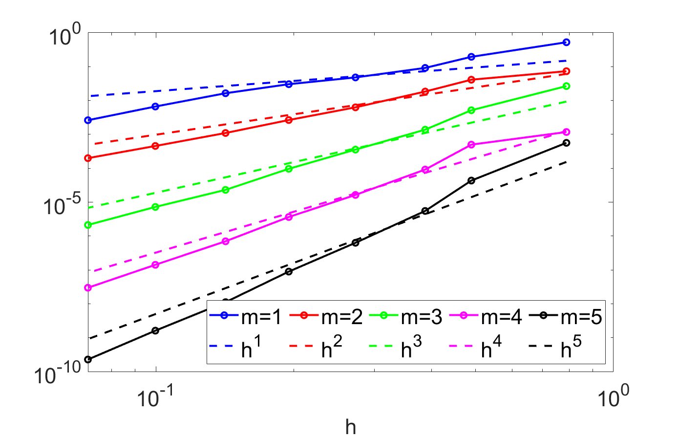
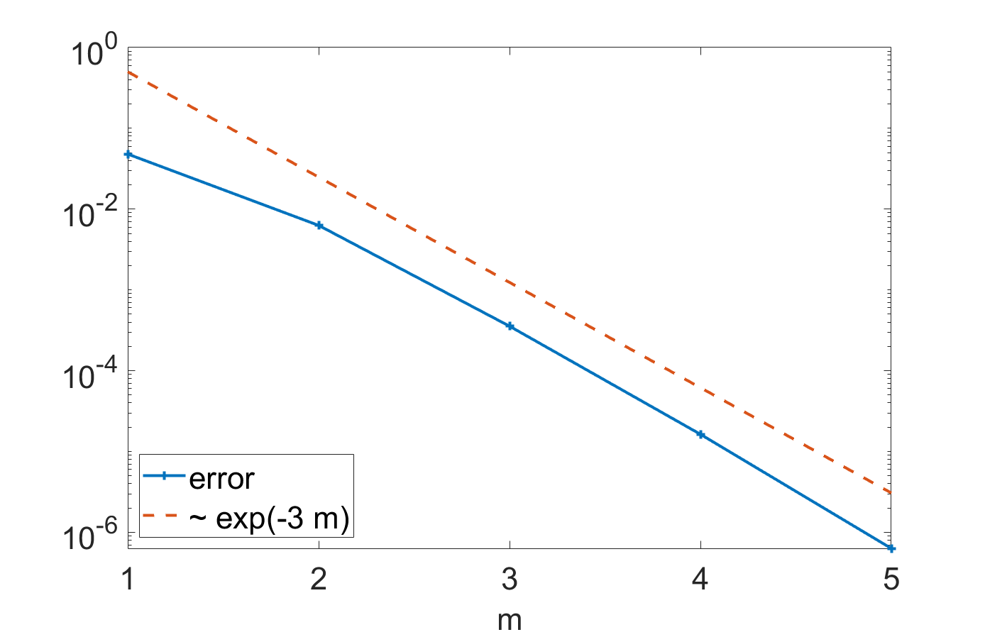
Figure 3: Test case 1. Left: computed errors in the energy norm (14) versus $h$, for different choices of the polynomial degree $m=1,2,3,4,5$. Right: computed errors in the energy norm (14) versus $m$, with $h=0.273$ (corresponding to $N=80$ polygons).

6.2 Test case 2: unsteady solution

We consider the rectangular domain $\Omega=\Omega_{\rm el}\cup\Omega_{\rm f}=(-1,0)\times(0,1)\cup(0,1)\times(0,1)$ of Section 6.1 and we introduce the following functions of time:

$$g_{\rm el}(t) =\cos(\eta t)-\sin(\eta t), \text{where }\eta=\frac{\mu_{\rm el}}{\mu_{\rm f}(1-\alpha_{\rm E})},$$

$$g_{\bm{u}}(t) =g_{\rm el}(t)-\frac{\dot{g}_{\rm el}(t)}{\eta}, g_{p}(t)=\frac{g_{\rm E}(t)+g_{\bm{u}}(t)}{2}.$$

A time-dependent exact solution of problem (1e)-(2f)-(3e) can be manufactured combining these functions with the steady solution introduced in Section 6.1:

$${\bm{d}}(x,y,t) =g_{\rm el}(t){\bm{d}}^{\text{steady}}(x,y), p_{\rm E}(x,y,t) =g_{\rm el}(t)p_{\rm E}^{\text{steady}}(x,y),$$ (23)

$${\bm{u}}(x,y,t) =g_{\bm{u}}(t){\bm{u}}^{\text{steady}}(x,y), p(x,y,t) =g_{p}(t)p^{\text{steady}}(x,y),$$

with suitable definitions of the source terms and boundary data. Again, we performed convergence tests setting $\alpha_{\rm E}=0.5$ andall other physical parameters to 1. We choose a time step $\Delta t=$1\text{⋅}{10}^{-3}\text{\,}\mathrm{s}$$ and a final time $T=5\,\Delta t$. We report the computed errors in Fig. 4 (log-log scale). As predicted by Theorem 4.2, we observe that the error in the energy norm decays at a rate proportional to $h^{m}$, for any $m\geq 1$. Moreover, even though not covered by our theoretical analysis, we observe exponential convergence of the error for fixed $h$ and increasing $m$. Finally, we observe that the value chosen for $\Delta t$ is small enough to prevent error saturation for the sequence of meshes considered in this test.

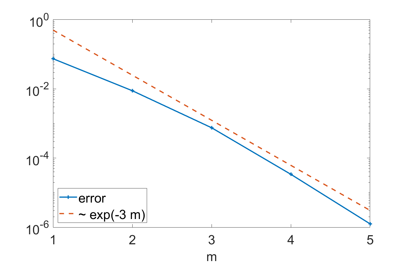
Figure 4: Test case 2. Left: computed errors in the energy norm (14) versus $h$, with different polynomial degrees $m$ (same for all variables). Right: computed errors in the energy norm (14) versus $m$, with $h=0.273$ corresponding to $N=80$ polygons.

7 Numerical results on a 2D slice of the brain

    
    

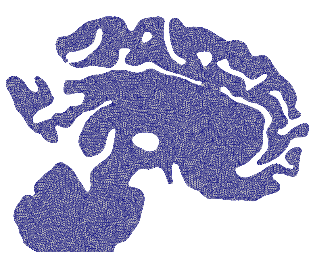
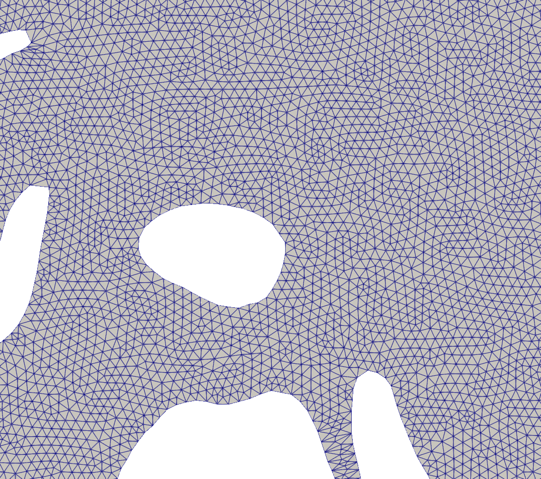
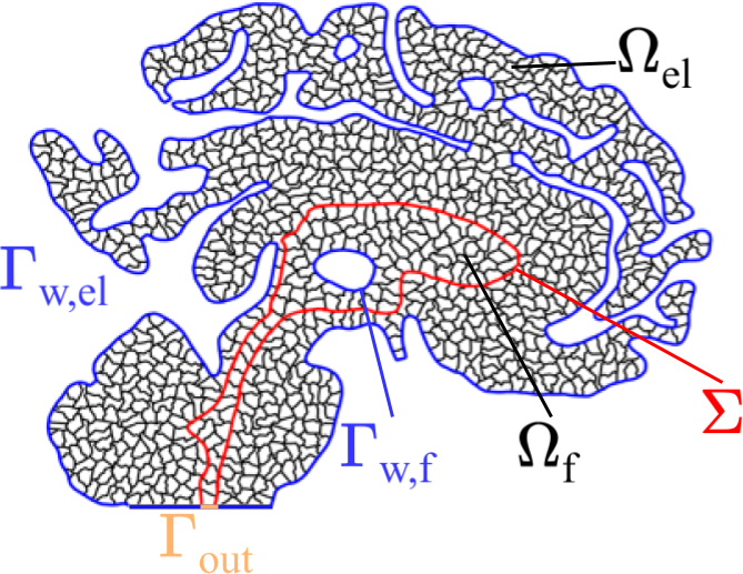
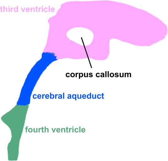
Figure 5: Triangular mesh of the 2D slice reconstructed from MRI (top left; zoom on top right to see the triangular elements), polygonal computational mesh obtained by agglomeration (bottom left), and topographic anatomy of the fluid domain $\Omega_{\rm f}$ (bottom right).

In this section, we demonstrate the capability of the proposed method for the solution of a realistic problem on a 2D slice of the brain and its ventricles, shown in Fig. 5. The geometry of the problem is based on structural Magnetic Resonance Images (MRI) available in the OASIS-3 database (https://oasis-brains.org) [56]. By means of Freesurfer (https://surfer.nmr.mgh.harvard.edu/) [44], a three-dimensional brain geometry was segmented, and then sliced along the sagittal plane by VMTK (vmtk.org) [5]. The resulting triangular 2D meshes of the cerebral tissue and of the brain ventricles surrounded by it are composed of 25847 and 3286 elements, respectively (see Fig. 5). Yet, the flexibility of the PolyDG method allows to employ meshes with elements of generic shape: by agglomeration, we can thus considerably reduce the number of mesh elements while retaining the same geometrical detail of the original triangular grid. We agglomerate the grid by means of ParMETIS (https://github.com/KarypisLab/ParMETIS) [54], obtaining the polygonal mesh shown in Fig. 5, consisting of 910 elements in $\mathscr{T}_{\rm el}$ and 101 in $\mathscr{T}_{\rm f}$. This agglomeration is performed separately for the two physical domains, to preserve geometrical accuracy at the interface $\Sigma$.

Aiming at reproducing conditions in the physiological regime, we set the data and parameters of problem (1e) as follows. We split the Dirichlet boundary $\Gamma_{\text{w}}$ into $\Gamma_{\text{w},{\rm el}}$ representing the dura mater membrane surrounding the brain tissue and the boundary $\Gamma_{\text{w},{\rm f}}$ of the corpus callosum (the whole in the center of Fig. 5). In the poroelastic problem, we consider only the compartment related to the extracellular CSF, namely $J=\{{\rm E}\}$, and we assume no flow ($\nabla p_{\rm E}\cdot{\bm{n}}_{\rm el}=0$) through the dura mater $\Gamma_{\text{w},{\rm el}}$. The source of extracellular CSF is given by $g_{\rm E}=$2\text{⋅}{10}^{-3}\text{\,}$\,\pi\sin(2\pi t)$\text{\,}{\mathrm{s}}^{-1}$,$ representing the variations in the interstitial CSF due to blood pulsation [57, 35, 32], with a period of $1\text{\,}\mathrm{s}$ representing a heartbeat. No additional external forces act on the poroelastic tissue or the ventricle flow, that is ${\bm{f}}_{\rm el}={\bm{f}}_{\rm f}={\bm{0}}$. No slip conditions ${\bm{u}}={\bm{0}}$ are enforced on $\Gamma_{\text{w},{\rm f}}$, while a no-stress condition $\overline{p}^{\text{out}}=0$ is imposed on the obex $\Gamma_{\text{out}}$ of the fourth ventricle, where the CSF would flow into the central canal of the spinal cord. Zero initial conditions are imposed on all variables and the values of the remaining physical parameters of the problem are reported in Table 1, with the slight modifications $\alpha_{\rm E}=0.49,\beta_{\rm E}^{\text{e}}=$0\text{\,}{\mathrm{m}}^{2}\text{⋅}{\mathrm{N}}^{-1}\text{⋅}{\mathrm{s}}^{-1}$$: these values are in the physiological range of the brain function [57, 35, 32]. For the PolyDG method we employ a polynomial degree $m=2$ for all variables, while for the time advancement based on Newmark’s ($\beta=0.25,\gamma=0.5$) and Crank-Nicolson’s ($\theta=0.5$) methods we use a time step $\Delta t=$1\text{⋅}{10}^{-2}\text{\,}\mathrm{s}$$ from $t_{0}=$0\text{\,}\mathrm{s}$$ to $T=$1\text{\,}\mathrm{s}$$.

Selected snapshots of the computed solutions are reported in Figs. 6 and 7. Due to the choice of a zero outlet pressure $\overline{p}^{\text{out}}$, pressures $p_{\rm E},p$ should be interpreted as pressure differences (w.r.t. the fourth ventricle outflow) rather than absolute pressure values. We notice that the amplitude of the brain displacement ${\bm{d}}$ is always below $0.2\text{\,}\mathrm{mm}$, thus justifying the choice of a linear elasticity modeling of the tissue, at least in the current settings. Due to such small displacements, the interstitial pressure $p_{\rm E}$ at the interface and the ventricle CSF pressure $p$ are substantially equal through the whole simulation timespan, in accordance with the interface conditions (3e). The ventricle pressure $p$ undergoes very small variations, which are better observable in Fig. 7. We can see that the CSF circulates in the third ventricle around the corpus callosum, whereas its flow through the cerebral aqueduct is always directed outwards, thus fulfilling its clearance function. This clearance occurs notwithstanding the fact that the source term $g_{\rm E}$ is negative in the second half of the timespan, and consequently the interstitial pressure $p_{\rm E}$ is lower than the outlet pressure $\overline{p}^{\text{out}}=0$: this effect is due to the inertial terms in the problem formulation, thus highlighting their importance in the model.

All the observations above are in general agreement with measurements and computational results in the literature, particularly in the magnitude of the displacement ${\bm{d}}$ and in the pressure difference between the third ventricle and the outflow [25, 32]. Some discrepancies can be observed in the overall range of $p_{\rm E}$ and the magnitude of ${\bm{u}}$, but they do not exceed one order of magnitude. These discrepancies may be due to the fact that the computational domain of the simulation presented here is a 2D slice of the brain, and does not include the lateral ventricles: simulations in three dimensions, capturing the complete geometry of the brain, are envisaged to address this issue.

Figure 6: Brain simulation of Section 7. Discrete tissue displacement ${\bm{d}}_{h}$ and pressures $p_{{\rm E},h},p_{h}$ in the whole domain $\Omega_{\rm el}\cup\Omega_{\rm f}$ at different times during a heartbeat. Same scale for $p_{{\rm E},h},p_{h}$.

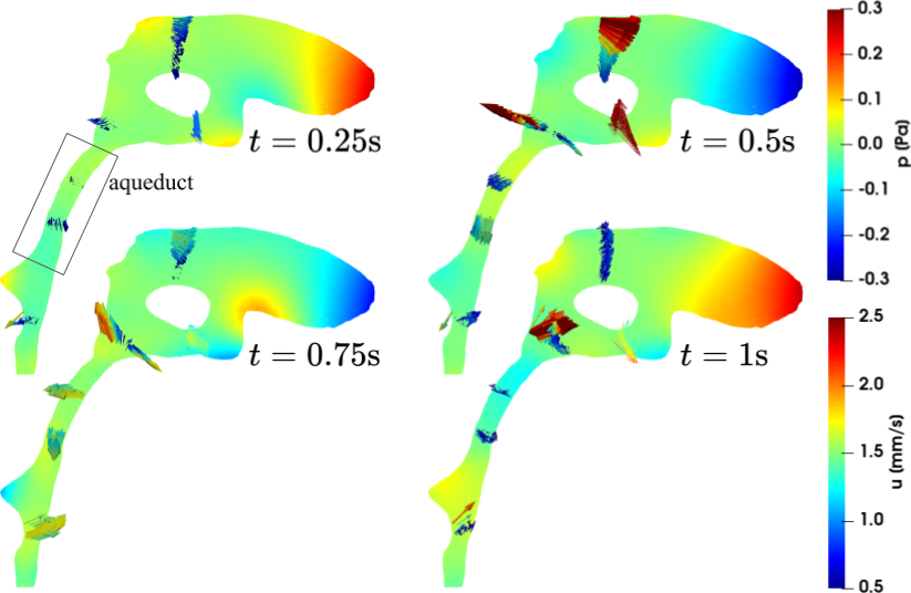
Figure 7: Brain simulation of Section 7. Velocity ${\bm{u}}_{h}$ and pressure $p_{h}$ in the brain ventricles $\Omega_{\rm f}$ at different times during a heartbeat. The cerebral aqueduct is indicated by the box.

8 Conclusions

We introduced a discontinuous Galerkin polytopal method for the discretization of a multiphysics fluid-mechanics model of the brain, encompassing a Multi-compartment Poro-Elastic (MPE) modeling of the tissue, perfused by blood and CSF, and Stokes’ flow of the CSF in the brain cavities. Our numerical method is particularly suitable for capturing the high geometrical complexity of the brain, thanks to the possibility of supporting high-order approximations and agglomerated grids. We proved stability and optimal error bounds for the semidiscrete formulation under standard assumptions in the PolyDG framework. Specific attention was paid to the modeling and numerical treatment of the interface conditions between the MPE and fluid domain. We implemented the method in our PolyDG library lymph [9].

We performed verification tests, validating the optimal order of convergence of our method with respect to the mesh element size and spectral convergence with respect to the polynomial degree. Then, we showed the capability of our computational model to represent the physiological clearance function of the CSF in physiological settings, on a two-dimensional sagittal slice of the brain and of its ventricles.

Several directions for further development of the present work should be addressed. First, in terms of modeling, nonlinear hyperelastic rheology could be considered to account for the extremely soft nature of the brain tissue [63, 27, 4]. This would require more detailed fluid-structure interaction conditions on the tissue-fluid interface, which have not been fully studied in the brain ventricles, but have been widely investigated in other biological systems such as the heart and blood vessels [67, 43, 52, 26, 46]. Second, to thoroughly analyze the effect of the complex brain geometry on waste clearance, the model could be applied to full three-dimensional geometries of different subjects. To this aim, suitable geometry reconstruction techniques based on MRI data should be employed, such as those developed in [68, 62, 70, 45, 47, 20, 17]. Third, to better represent the effect of blood pulsation on CSF flow (here modeled by a homogeneous CSF generation term), the blood compartments of the MPE model should be coupled to models of the main brain arteries [53, 60]. Finally, the coupling of the model proposed here with a suitable description of the generation, aggregation, and transport of misfolded proteins such as amyloid-$\beta$ and tau, would allow the investigation of their clearance in different physiological and pathological conditions [36, 37]. This would entail the development of numerical methods able to account for very different time scales, since the model presented here is defined on the scale of seconds (characteristic of blood pulsation) while prion aggregation and neurodegeneration occur over a timespan of decades.

Appendix A Continuity and coercivity in the discrete spaces

We collect the continuity and coercivity results of [35, 14] in the following Lemma, which is instrumental to the proofs of stability (Theorem 4.1) and convergence (Theorem 4.2) of our numerical method (10).

Lemma A.1

Under Assumption 4.1, the forms of (7) are continuous over the discrete spaces:

$$|\mathcal{A}_{\rm el}({\bm{d}},{\bm{w}})| \lesssim|\mkern-1.5mu|{\bm{d}}|\mkern-1.5mu|_{{\rm DG},{\rm D}}|\mkern-1.5mu|{\bm{w}}|\mkern-1.5mu|_{{\rm DG},{\rm D}} \forall{\bm{d}},{\bm{w}}\in{\bm{W}}^{\rm DG}_{h},$$

$$|\mathcal{A}_{\rm j}(p_{\rm j},q_{\rm j})| \lesssim|\mkern-1.5mu|p_{\rm j}|\mkern-1.5mu|_{{\rm DG},{\rm P}_{\rm j}}|\mkern-1.5mu|q_{\rm j}|\mkern-1.5mu|_{{\rm DG},{\rm P}_{\rm j}} \forall p_{\rm j},q_{\rm j}\in Q^{\rm DG}_{{\rm j},h},\quad{\rm j}\in J,$$

$$\left|\sum_{{\rm j}\in J}\mathcal{C}_{\rm j}(\{p_{\rm k}\}_{{\rm k}\in J},q_{\rm j})\right| \lesssim\sum_{{\rm j},{\rm k}\in J}|\mkern-1.5mu|p_{\rm k}|\mkern-1.5mu|_{{\rm DG},{\rm P}_{\rm k}}|\mkern-1.5mu|q_{\rm j}|\mkern-1.5mu|_{{\rm DG},{\rm P}_{\rm j}} \forall p_{\rm k},\in Q^{\rm DG}_{{\rm k},h},q_{\rm j}\in Q^{\rm DG}_{{\rm j},h},\quad{\rm j},{\rm k}\in J,$$

$$|\mathcal{B}_{\rm j}(q_{\rm j},{\bm{w}})| \lesssim|\mkern-1.5mu|q_{\rm j}|\mkern-1.5mu|_{{\rm DG},{\rm P}_{\rm j}}|\mkern-1.5mu|{\bm{w}}|\mkern-1.5mu|_{{\rm DG},{\rm D}} \forall{\bm{w}}\in{\bm{W}}^{\rm DG}_{h},q_{\rm j}\in Q^{\rm DG}_{{\rm j},h},\quad{\rm j}\in J,$$

$$|\mathcal{A}_{\rm f}({\bm{u}},{\bm{v}})| \lesssim|\mkern-1.5mu|{\bm{u}}|\mkern-1.5mu|_{{\rm DG},{\rm U}}|\mkern-1.5mu|{\bm{v}}|\mkern-1.5mu|_{{\rm DG},{\rm U}} \forall{\bm{u}},{\bm{v}}\in{\bm{V}}^{\rm DG}_{h},$$

$$|\mathcal{B}(q,{\bm{v}})| \lesssim|\mkern-1.5mu|q|\mkern-1.5mu|_{{\rm DG},{\rm P}_{\rm f}}|\mkern-1.5mu|{\bm{v}}|\mkern-1.5mu|_{{\rm DG},{\rm U}} \forall{\bm{v}}\in{\bm{V}}^{\rm DG}_{h},q\in Q^{\rm DG}_{h},$$

Moreover, provided that the penalty constants are chosen sufficiently large, the following coercivity and inf-sup inequalities hold (for any ${\rm j}\in J$):

$$\mathcal{A}_{\rm el}({\bm{w}},{\bm{w}})\gtrsim|\mkern-1.5mu|{\bm{w}}|\mkern-1.5mu|_{{\rm DG},{\rm D}}^{2}\qquad\forall{\bm{w}}\in{\bm{W}}^{\rm DG}_{h},$$

$$\mathcal{A}_{\rm f}({\bm{v}},{\bm{v}})\gtrsim|\mkern-1.5mu|{\bm{v}}|\mkern-1.5mu|_{{\rm DG},{\rm U}}^{2}\qquad\forall{\bm{v}}\in{\bm{V}}^{\rm DG}_{h},$$

$$\sum_{{\rm j}\in J}\mathcal{C}_{\rm j}(\{q_{\rm k}\}_{{\rm k}\in J},q_{\rm j})\gtrsim\sum_{{\rm j}\in J}\|\sqrt{\beta_{\rm j}^{\text{e}}}q_{\rm j}\|_{\text{DG},P_{\rm j}}^{2}\quad\text{and}\quad\mathcal{A}_{\rm j}(q_{\rm j},q_{\rm j})\gtrsim|\mkern-1.5mu|q_{\rm j}|\mkern-1.5mu|_{{\rm DG},{\rm P}_{\rm j}}^{2}\quad\forall q_{\rm j}\in Q^{\rm DG}_{{\rm j},h},\ {\rm j}\in J,$$

$$\sup_{{\bm{v}}\in{\bm{V}}^{\rm DG}_{h}\setminus\{0\}}\frac{\mathcal{B}_{\rm f}(q,{\bm{v}})}{|\mkern-1.5mu|{\bm{v}}|\mkern-1.5mu|_{{\rm DG},{\rm U}}}+\sqrt{\mathcal{S}(q,q)}\geq\beta_{{\rm f},h}\|q\|_{\Omega_{\rm f}}\qquad\forall q\in Q^{\rm DG}_{h},$$

where $\beta_{{\rm f},h}$ is the discrete inf-sup constant [14].

Appendix B Proof of Lemma 4.1

Let $q\in H^{2}(\mathscr{T}_{h,{\rm el}}),{\bm{w}}\in H^{2}(\mathscr{T}_{h,{\rm el}}),{\bm{v}}\in H^{2}(\mathscr{T}_{h,{\rm f}})$, and $q\in Q^{\rm DG}_{{\rm E},h},{\bm{w}}_{h}\in{\bm{W}}^{\rm DG}_{h},{\bm{v}}_{h}\in{\bm{V}}^{\rm DG}_{h}$. For any $F\in\mathscr{F}_{h}^{\Sigma}$, we denote by $K_{\rm el}^{F}$ and $K_{\rm f}^{F}$ the elements of $\mathscr{T}_{h,{\rm el}}$ and $\mathscr{T}_{h,{\rm f}}$, respectively, sharing $F$ in their boundary. Then,

$$|\mathcal{J}(q,{\bm{w}}_{h},{\bm{v}}_{h})| \leq\sum_{F\in\mathscr{F}_{h}^{\Sigma}}\left(\left|\int_{F}q\,{\bm{w}}_{h}\cdot{\bm{n}}_{\rm el}\right|+\left|\int_{F}q\,{\bm{v}}_{h}\cdot{\bm{n}}_{\rm f}\right|\right)$$

$$\lesssim\sum_{F\in\mathscr{F}_{h}^{\Sigma}}\left(\|\eta^{1/2}q\|_{F}\|\eta^{-1/2}{\bm{w}}_{h}\|_{F}+\|\gamma_{p}^{-1/2}q\|_{F}\|\gamma_{p}^{1/2}{\bm{v}}_{h}\|_{F}\right)$$

$$\overset{\framebox{TR}}{\lesssim}\sum_{F\in\mathscr{F}_{h}^{\Sigma}}\left(\|\eta^{1/2}q\|_{F}\cancel{h_{K_{\rm el}^{F}}^{1/2}}\cancel{{h_{K_{\rm el}^{F}}^{-1/2}}}\|{\bm{w}}_{h}\|_{K_{\rm el}^{F}}+\|\gamma_{p}^{-1/2}q\|_{F}\cancel{h_{K_{\rm f}^{F}}^{1/2}}\cancel{{h_{K_{\rm f}^{F}}^{-1/2}}}\|{\bm{v}}_{h}\|_{K_{\rm f}^{F}}\right)$$

$$\leq\|\eta^{1/2}q\|_{\mathscr{F}_{h}^{\Sigma}}|\mkern-1.5mu|{\bm{w}}_{h}|\mkern-1.5mu|_{{\rm DG},{\rm D}}+\|\gamma_{p}^{-1/2}q\|_{\mathscr{F}_{h}^{\Sigma}}|\mkern-1.5mu|{\bm{v}}_{h}|\mkern-1.5mu|_{{\rm DG},{\rm U}},$$

where, in line TR, we have used the inverse trace inequality (18) and the fact that $\eta|_{K}\sim h_{K}^{-1}\ \forall K\in\mathscr{T}_{h,{\rm el}}$ and $\gamma_{p}|_{K}\sim h_{K}\ \forall K\in\mathscr{T}_{h,{\rm f}}$. An analogous argument (using $\gamma_{\bm{v}}^{1/2}$ in place of $\gamma_{p}^{-1/2}$) allows to control $|J(q_{h},{\bm{w}},{\bm{v}})|$, thus concluding the proof.

Appendix C Proof of Theorem 4.2

In this section, we prove the optimal convergence estimate stated in Theorem 4.2. This result is based on the inverse trace inequality (18), on Lemma 4.1 and on the following continuity results (proved in [10, 8, 14]), which extend Lemma A.1 to consider also non-discrete functions:

Lemma C.1

Under the same assumptions of Lemma A.1, the following inequalities hold:

$$|\mathcal{A}_{\rm el}({\bm{d}},{\bm{w}}_{h})| \lesssim|\mkern-1.5mu|\mkern-1.5mu|{\bm{d}}|\mkern-1.5mu|\mkern-1.5mu|_{{\rm D}}|\mkern-1.5mu|{\bm{w}}_{h}|\mkern-1.5mu|_{{\rm DG},{\rm D}} \forall{\bm{d}}\in[H^{2}(\mathscr{T}_{h,{\rm el}})]^{d},{\bm{w}}_{h}\in{\bm{W}}^{\rm DG}_{h},$$

$$|\mathcal{A}_{\rm j}(p_{\rm j},q_{{\rm j},h})| \lesssim|\mkern-1.5mu|\mkern-1.5mu|p_{\rm j}|\mkern-1.5mu|\mkern-1.5mu|_{{\rm P}_{\rm j}}|\mkern-1.5mu|q_{{\rm j},h}|\mkern-1.5mu|_{{\rm DG},{\rm P}_{\rm j}} \forall p_{\rm j}\in H^{2}(\mathscr{T}_{h,{\rm el}}),q_{{\rm j},h}\in Q^{\rm DG}_{{\rm j},h},\quad\forall{\rm j}\in J,$$

$$|\mathcal{B}_{\rm j}(q_{{\rm j},h},{\bm{w}})| \lesssim|\mkern-1.5mu|q_{{\rm j},h}|\mkern-1.5mu|_{{\rm DG},{\rm P}_{\rm j}}|\mkern-1.5mu|\mkern-1.5mu|{\bm{w}}|\mkern-1.5mu|\mkern-1.5mu|_{{\rm D}} \forall{\bm{w}}\in[H^{2}(\mathscr{T}_{h,{\rm el}})]^{d},q_{{\rm j},h}\in Q^{\rm DG}_{{\rm j},h},\quad\forall{\rm j}\in J,$$

$$|\mathcal{B}_{\rm j}(q_{\rm j},{\bm{w}}_{h})| \lesssim|\mkern-1.5mu|\mkern-1.5mu|q_{\rm j}|\mkern-1.5mu|\mkern-1.5mu|_{{\rm P}_{\rm j}}|\mkern-1.5mu|{\bm{w}}_{h}|\mkern-1.5mu|_{{\rm DG},{\rm D}} \forall{\bm{w}}_{h}\in{\bm{W}}^{\rm DG}_{h},q_{\rm j}\in H^{2}(\mathscr{T}_{h,{\rm el}}),\quad\forall{\rm j}\in J,$$

$$|\mathcal{A}_{\rm f}({\bm{u}},{\bm{v}}_{h})| \lesssim|\mkern-1.5mu|\mkern-1.5mu|{\bm{u}}|\mkern-1.5mu|\mkern-1.5mu|_{{\rm U}}|\mkern-1.5mu|{\bm{v}}_{h}|\mkern-1.5mu|_{{\rm DG},{\rm U}} \forall{\bm{u}}\in[H^{2}(\mathscr{T}_{h,{\rm f}})]^{d},{\bm{v}}_{h}\in{\bm{V}}^{\rm DG}_{h},$$

$$|\mathcal{B}_{\rm f}(q_{h},{\bm{v}})| \lesssim|\mkern-1.5mu|q_{h}|\mkern-1.5mu|_{{\rm DG},{\rm P}_{\rm f}}|\mkern-1.5mu|\mkern-1.5mu|{\bm{v}}|\mkern-1.5mu|\mkern-1.5mu|_{{\rm U}} \forall{\bm{v}}\in[H^{2}(\mathscr{T}_{h,{\rm f}})]^{d},q_{h}\in Q^{\rm DG}_{h},$$

$$|\mathcal{B}_{\rm f}(q,{\bm{v}}_{h})| \lesssim|\mkern-1.5mu|\mkern-1.5mu|q|\mkern-1.5mu|\mkern-1.5mu|_{{\rm P}_{\rm f}}|\mkern-1.5mu|{\bm{v}}_{h}|\mkern-1.5mu|_{{\rm DG},{\rm U}} \forall{\bm{v}}_{h}\in{\bm{V}}^{\rm DG}_{h},q\in H^{1}(\mathscr{T}_{h,{\rm f}}).$$

We are now ready to prove our optimal convergence result. Proof.  (Theorem 4.2) Using the interpolators defined in Lemma 4.2, we split the error ${\bm{e}}^{\bm{d}}={\bm{e}}^{\bm{d}}_{I}-{\bm{e}}^{\bm{d}}_{h}$ into an interpolation error ${\bm{e}}^{\bm{d}}_{I}={\bm{d}}-{\bm{d}}_{I}\in[H^{m+1}(\mathscr{T}_{h,{\rm el}})]^{d}$ and an approximation error ${\bm{e}}^{\bm{d}}_{h}={\bm{d}}_{h}-{\bm{d}}_{I}\in{\bm{W}}^{\rm DG}_{h}$. An analogous notation is introduced for the errors $e^{P_{\rm j}}\ \forall{\rm j}\in J,{\bm{e}}^{\bm{u}},e^{P_{\rm f}}$. We fix a time $t\in(0,T]$ and we proceed similarly to [35], namely we subtract equation (10) from (6), tested against $(\partial_{t}{\bm{e}}^{\bm{d}}_{h},\{e^{P_{{\rm j}}}_{h}\}_{{\rm j}\in J},{\bm{e}}^{\bm{u}}_{h},e^{P_{\rm f}}_{h})$, thus obtaining

$$(\rho_{\rm el}\partial_{tt}^{2}{\bm{e}}^{\bm{d}} ,\partial_{t}{\bm{e}}^{\bm{d}}_{h})_{\Omega_{\rm el}}+\mathcal{A}_{\rm el}({\bm{e}}^{\bm{d}},\partial_{t}{\bm{e}}^{\bm{d}}_{h})+\sum_{{\rm k}\in J}\mathcal{B}_{\rm k}(e^{P_{\rm k}},\partial_{t}{\bm{e}}^{\bm{d}}_{h})$$

$$+\sum_{{\rm j}\in J}\left[(c_{\rm j}\partial_{t}e^{P_{\rm j}},e^{P_{\rm j}}_{h})_{\Omega_{\rm el}}+\mathcal{A}_{\rm j}(e^{P_{\rm j}},e^{P_{\rm j}}_{h})+\mathcal{C}_{\rm j}(\{e^{P_{\rm k}}\}_{{\rm k}\in J},e^{P_{\rm j}}_{h})-\mathcal{B}_{\rm j}(e^{P_{\rm j}}_{h},\partial_{t}{\bm{e}}^{\bm{d}})\right]$$

$$+(\rho_{\rm f}\partial_{t}{\bm{e}}^{\bm{u}},{\bm{u}}_{h})_{\Omega_{\rm f}}+\mathcal{A}_{\rm f}({\bm{e}}^{\bm{u}},{\bm{e}}^{\bm{u}}_{h})+\mathcal{B}_{\rm f}(e^{P_{\rm f}},{\bm{e}}^{\bm{u}}_{h})-\mathcal{B}_{\rm f}(e^{P_{\rm f}}_{h},{\bm{e}}^{\bm{u}})+\mathcal{S}(e^{P_{\rm f}},e^{P_{\rm f}}_{h})$$

$$+\mathcal{J}(e^{P_{\rm E}},\partial_{t}{\bm{e}}^{\bm{d}}_{h},{\bm{e}}^{\bm{u}}_{h})-\mathcal{J}(e^{P_{{\rm E}}}_{h},\partial_{t}{\bm{e}}^{\bm{d}},{\bm{e}}^{\bm{u}})=0.$$

According to the splitting introduced above, we separate the terms depending only on the discrete approximation errors from those involving the interpolation errors. Then, integrating in time from $0$ to $t$ and proceeding as in the proof of Theorem 4.1, the coercivity inequalities of Lemma A.1 yield

$$\| \sqrt{\rho_{\rm el}}\partial_{t}{\bm{e}}^{\bm{d}}_{h}\|_{\Omega_{\rm el}}^{2}+|\mkern-1.5mu|{\bm{e}}^{\bm{d}}_{h}|\mkern-1.5mu|_{{\rm DG},{\rm D}}^{2}+\sum_{{\rm k}\in J}\left[\|\sqrt{c_{\rm k}}e^{P_{\rm k}}_{h}\|_{\Omega_{\rm el}}^{2}+\int_{0}^{t}\left(|\mkern-1.5mu|e^{P_{\rm k}}_{h}|\mkern-1.5mu|_{{\rm DG},{\rm P}_{\rm k}}^{2}+\|\sqrt{\beta^{e}_{\rm k}}e^{P_{\rm k}}_{h}\|_{\Omega_{\rm el}}^{2}\right)ds\right]$$ (24)

$$\qquad+\|\sqrt{\rho_{\rm f}}{\bm{e}}^{\bm{u}}_{h}\|_{\Omega_{\rm f}}^{2}+\int_{0}^{t}\alpha\left(|\mkern-1.5mu|{\bm{e}}^{\bm{u}}_{h}|\mkern-1.5mu|_{{\rm DG},{\rm U}}^{2}+|\mkern-1.5mu|e^{P_{\rm f}}_{h}|\mkern-1.5mu|_{{\rm DG},{\rm P}_{\rm f}}^{2}\right)ds$$

$$\qquad+\int_{0}^{t}\left[\cancel{J(e^{P_{\rm E}}_{h},\partial_{t}{\bm{e}}^{\bm{d}}_{h},{\bm{e}}^{\bm{u}}_{h})}-\cancel{J(e^{P_{\rm E}}_{h},\partial_{t}{\bm{e}}^{\bm{d}}_{h},{\bm{e}}^{\bm{u}}_{h})}\right]ds$$

$$\lesssim\int_{0}^{t}(\rho_{\rm el}\partial_{tt}^{2}{\bm{e}}^{\bm{d}}_{I},\partial_{t}{\bm{e}}^{\bm{d}}_{h})_{\Omega_{\rm el}}ds+\mathcal{A}_{\rm el}({\bm{e}}^{\bm{d}}_{I},{\bm{e}}^{\bm{d}}_{h})-\int_{0}^{t}\mathcal{A}_{\rm el}(\partial_{t}{\bm{e}}^{\bm{d}}_{I},{\bm{e}}^{\bm{d}}_{h})ds$$

$$\qquad+\sum_{{\rm k}\in J}\int_{0}^{t}\left[(c_{\rm k}\partial_{t}e^{P_{\rm k}}_{I},e^{P_{\rm k}}_{h})_{\Omega_{\rm el}}+\mathcal{A}_{\rm k}(e^{P_{\rm k}}_{I},e^{P_{\rm k}}_{h})+\mathcal{C}_{\rm k}(\{e^{P_{\rm j}}_{I}\}_{{\rm j}\in J},e^{P_{\rm k}}_{h})\right]ds$$

$$\qquad+\sum_{{\rm k}\in J}\mathcal{B}_{\rm k}(e^{P_{\rm k}}_{I},{\bm{e}}^{\bm{d}}_{h})-\sum_{{\rm k}\in J}\int_{0}^{t}\left[\mathcal{B}_{\rm k}(e^{P_{\rm k}}_{I},\partial_{t}{\bm{e}}^{\bm{d}}_{h})+\mathcal{B}_{\rm k}(e^{P_{\rm k}}_{h},\partial_{t}{\bm{e}}^{\bm{d}}_{I})\right]ds$$

$$\qquad+\int_{0}^{t}\left[(\rho_{\rm f}\partial_{t}{\bm{e}}^{\bm{u}}_{I},{\bm{e}}^{\bm{u}}_{h})_{\Omega_{\rm f}}+\mathcal{A}_{\rm f}({\bm{e}}^{\bm{u}}_{I},{\bm{e}}^{\bm{u}}_{h})+\mathcal{B}_{\rm f}(e^{P_{\rm f}}_{I},{\bm{e}}^{\bm{u}}_{u})-\mathcal{B}_{\rm f}(e^{P_{\rm f}}_{h},{\bm{e}}^{\bm{u}}_{I})+\mathcal{S}(e^{P_{\rm f}}_{I},e^{P_{\rm f}}_{h})\right]ds$$

$$\qquad+\int_{0}^{t}\left[J(e^{P_{\rm E}}_{I},\partial_{t}{\bm{e}}^{\bm{d}}_{h},{\bm{e}}^{\bm{u}}_{h})-J(e^{P_{\rm E}}_{h},\partial_{t}{\bm{e}}^{\bm{d}}_{I},{\bm{e}}^{\bm{u}}_{I})\right]ds,$$

where no contribution arises from the initial conditions, due to the hypotheses. Using Lemmas 4.1 and C.1 and the inequality

$$\sum_{{\rm k}\in J}|C_{\rm k}(\{e_{I}^{P_{\rm j}}\}_{{\rm j}\in J}.e^{P_{\rm k}}_{h})|\lesssim\sum_{{\rm j},{\rm k}\in J}\|c_{\rm j}^{-1/2}e_{I}^{P_{\rm j}}\|_{\Omega_{\rm el}}\|\sqrt{c_{\rm k}}e_{h}^{P_{\rm k}}\|_{\Omega_{\rm el}}\lesssim\sum_{{\rm j},{\rm k}\in J}|\mkern-1.5mu|\mkern-1.5mu|e_{I}^{P_{\rm j}}|\mkern-1.5mu|\mkern-1.5mu|_{{\rm P}_{\rm j}}\|\sqrt{c_{\rm k}}e_{h}^{P_{\rm k}}\|_{\Omega_{\rm el}}$$

on the right-hand side of (24) yields

$$|\mkern-1.5mu|({\bm{e}}^{\bm{d}}_{h},\{e^{P_{\rm j}}_{h}\}_{{\rm j}\in J},{\bm{e}}^{\bm{u}}_{h},e^{P_{\rm f}}_{h})|\mkern-1.5mu|_{{\rm EN},t}^{2}$$ (25)

$$\qquad\lesssim|\mkern-1.5mu|\mkern-1.5mu|{\bm{e}}^{\bm{d}}_{I}(t)|\mkern-1.5mu|\mkern-1.5mu|_{{\rm D}}|\mkern-1.5mu|{\bm{e}}^{\bm{d}}_{h}(t)|\mkern-1.5mu|_{{\rm DG},{\rm D}}+\int_{0}^{t}\left[\|\sqrt{\rho_{\rm el}}\partial_{tt}^{2}{\bm{e}}^{\bm{d}}_{I}(s)\|_{\Omega_{\rm el}}\|\sqrt{\rho_{\rm el}}\partial_{t}{\bm{e}}^{\bm{d}}_{h}(s)\|_{\Omega_{\rm el}}\right.$$

$$\qquad\qquad\qquad\qquad\qquad\qquad\qquad\qquad\qquad\left.+|\mkern-1.5mu|\mkern-1.5mu|\partial_{t}{\bm{e}}^{\bm{d}}_{I}(s)|\mkern-1.5mu|\mkern-1.5mu|_{{\rm D}}|\mkern-1.5mu|{\bm{e}}^{\bm{d}}_{h}(s)|\mkern-1.5mu|_{{\rm DG},{\rm D}}\right]ds$$

$$\qquad\qquad+\sum_{{\rm k}\in J}\left[|\mkern-1.5mu|\mkern-1.5mu|e^{P_{\rm k}}_{I}(t)|\mkern-1.5mu|\mkern-1.5mu|_{{\rm P}_{\rm k}}|\mkern-1.5mu|{\bm{e}}^{\bm{d}}_{h}(t)|\mkern-1.5mu|_{{\rm DG},{\rm D}}+\int_{0}^{t}\|\sqrt{c_{\rm k}}\partial_{t}e^{P_{\rm k}}_{I}(s)\|_{\Omega_{\rm el}}\|\sqrt{c_{\rm k}}e^{P_{\rm k}}_{h}(s)\|_{\Omega_{\rm el}}ds\right]$$

$$\qquad\qquad+\sum_{{\rm k}\in J}\int_{0}^{t}\left[|\mkern-1.5mu|\mkern-1.5mu|e^{P_{\rm k}}_{I}(s)|\mkern-1.5mu|\mkern-1.5mu|_{{\rm P}_{\rm k}}|\mkern-1.5mu|e^{P_{\rm k}}_{h}(s)|\mkern-1.5mu|_{{\rm DG},{\rm P}_{\rm k}}+|\mkern-1.5mu|\mkern-1.5mu|e^{P_{\rm k}}_{I}(s)|\mkern-1.5mu|\mkern-1.5mu|_{{\rm P}_{\rm k}}|\mkern-1.5mu|\partial_{t}{\bm{e}}^{\bm{d}}_{h}(s)|\mkern-1.5mu|_{{\rm DG},{\rm D}}\right]ds$$

$$\qquad\qquad+\sum_{{\rm k}\in J}\int_{0}^{t}\left[|\mkern-1.5mu|e^{P_{\rm k}}_{h}(s)|\mkern-1.5mu|_{{\rm DG},{\rm P}_{\rm k}}|\mkern-1.5mu|\mkern-1.5mu|\partial_{t}{\bm{e}}^{\bm{d}}_{I}(s)|\mkern-1.5mu|\mkern-1.5mu|_{{\rm D}}+\sum_{{\rm j}\in J}|\mkern-1.5mu|\mkern-1.5mu|e^{P_{\rm j}}_{I}(s)|\mkern-1.5mu|\mkern-1.5mu|_{{\rm P}_{\rm j}}\|\sqrt{c_{\rm k}}e^{P_{\rm k}}_{h}(s)\|_{\Omega_{\rm el}}\right]ds$$

$$\qquad\qquad+\int_{0}^{t}[\|\sqrt{\rho_{\rm f}}\partial_{t}{\bm{e}}^{\bm{u}}_{I}(s)\|_{\Omega_{\rm f}}\|{\bm{e}}^{\bm{u}}_{h}(s)\|_{\Omega_{\rm f}}+|\mkern-1.5mu|\mkern-1.5mu|{\bm{e}}^{\bm{u}}_{I}(s)|\mkern-1.5mu|\mkern-1.5mu|_{{\rm U}}|\mkern-1.5mu|{\bm{e}}^{\bm{u}}_{h}(s)|\mkern-1.5mu|_{{\rm DG},{\rm U}}$$

$$\qquad\qquad\qquad\qquad\qquad\qquad\qquad\qquad\qquad+|\mkern-1.5mu|\mkern-1.5mu|e^{P_{\rm f}}_{I}(s)|\mkern-1.5mu|\mkern-1.5mu|_{{\rm P}_{\rm f}}|\mkern-1.5mu|{\bm{e}}^{\bm{u}}_{h}(s)|\mkern-1.5mu|_{{\rm DG},{\rm U}}]ds$$

$$\qquad\qquad+\int_{0}^{t}\left[|\mkern-1.5mu|e^{P_{\rm f}}_{h}(s)|\mkern-1.5mu|_{{\rm DG},{\rm P}_{\rm f}}|\mkern-1.5mu|\mkern-1.5mu|{\bm{e}}^{\bm{u}}_{I}(s)|\mkern-1.5mu|\mkern-1.5mu|_{{\rm U}}+\sqrt{\mathcal{S}(e^{P_{\rm f}}_{I}(s),e^{P_{\rm f}}_{I}(s))}\sqrt{\mathcal{S}(e^{P_{\rm f}}_{h}(s),e^{P_{\rm f}}_{h}(s))}\right]ds$$

$$\qquad\qquad+\int_{0}^{t}\left[\|\eta^{1/2}e^{P_{\rm E}}_{I}\|_{\mathscr{F}_{h}^{\Sigma}}|\mkern-1.5mu|\partial_{t}{\bm{e}}^{\bm{d}}_{h}|\mkern-1.5mu|_{{\rm DG},{\rm D}}+\|\gamma_{p}^{-1/2}e^{P_{\rm E}}_{I}\|_{\mathscr{F}_{h}^{\Sigma}}|\mkern-1.5mu|{\bm{e}}^{\bm{u}}_{h}|\mkern-1.5mu|_{{\rm DG},{\rm U}}\right]ds$$

$$\qquad\qquad+\int_{0}^{t}\left[|\mkern-1.5mu|e^{P_{\rm E}}_{h}|\mkern-1.5mu|_{{\rm DG},{\rm P}_{\rm E}}\left(\|\eta^{1/2}\partial_{t}{\bm{e}}^{\bm{d}}_{I}\|_{\mathscr{F}_{h}^{\Sigma}}+\|\gamma_{\bm{v}}^{1/2}{\bm{e}}^{\bm{u}}_{I}\|_{\mathscr{F}_{h}^{\Sigma}}\right)\right]ds.$$

Regarding the interface terms, we can observe that the choice of $\eta,\gamma_{\bm{v}},\gamma_{p}$ made in (8) implies that $\eta,\gamma_{\bm{v}},\gamma_{p}^{-1}$ scale as $h_{K}$ in each element $K\in\mathscr{T}_{h}$. Thus, thanks to Lemma 4.2, we obtain

$$\|\eta^{1/2}e_{I}^{P_{\rm E}}\|_{\mathscr{F}_{h}^{\Sigma}} \lesssim\sum_{K\in\mathscr{T}_{h,{\rm el}}}\|\eta\|_{L^{\infty}(K)}^{1/2}\|h_{K}^{m+1/2}\|\mathcal{E}_{K}p_{\rm E}\|_{H^{m+1}(\widehat{K})}\lesssim\sum_{K\in\mathscr{T}_{h,{\rm el}}}h_{K}^{m}\|\mathcal{E}_{K}p_{\rm E}\|_{H^{m+1}(\widehat{K})},$$

and similar optimal estimates for the other interpolation errors at the interface appearing in the last two lines of (25).

By Cauchy-Schwarz’s and Young’s inequalities, all the terms involving the discrete errors ${\bm{e}}^{\bm{d}}_{h},e^{P_{\rm j}}_{h},{\bm{e}}^{\bm{u}}_{h},e^{P_{\rm f}}_{h}$ on the right-hand side of (25) can be moved to the left-hand side, whereas the interpolation errors ${\bm{e}}^{\bm{d}}_{I},e^{P_{\rm j}}_{I},{\bm{e}}^{\bm{u}}_{I},e^{P_{\rm f}}_{I}$ can be controlled by the estimates of Lemma 4.2, yielding

$$|\mkern-1.5mu|({\bm{e}}^{\bm{d}}_{h},\{e^{P_{\rm j}}_{h}\}_{{\rm j}\in J},{\bm{e}}^{\bm{u}}_{h},e^{P_{\rm f}}_{h})|\mkern-1.5mu|_{{\rm EN},t}^{2}$$ (26)

$$\qquad\lesssim\sum_{K\in\mathscr{T}_{h,{\rm el}}}\frac{h_{K}^{2m}}{m}\left\{\|\mathcal{E}_{K}{\bm{d}}(t)\|_{[H^{m+1}(\widehat{K})]^{d}}^{2}+\sum_{{\rm k}\in J}\|\mathcal{E}_{K}p_{\rm k}(t)\|_{H^{m+1}(\widehat{K})}^{2}\right.$$

$$\qquad\qquad\quad\left.\qquad\quad+\int_{0}^{t}\left[\|\mathcal{E}_{K}\partial_{t}{\bm{d}}(s)\|_{[H^{m+1}(\widehat{K})]^{d}}^{2}+\|\mathcal{E}_{K}\partial_{tt}^{2}{\bm{d}}(s)\|_{[H^{m+1}(\widehat{K})]^{d}}^{2}\phantom{\sum_{k\in J}}\right.\right.$$

$$\qquad\qquad\qquad\left.\qquad\quad\left.+\sum_{k\in J}\left(\|\mathcal{E}_{K}p_{\rm k}(s)\|_{H^{m+1}(\widehat{K})}^{2}+\|\mathcal{E}_{K}\partial_{t}p_{\rm k}(s)\|_{H^{m+1}(\widehat{K})}^{2}\right)\right]ds\right\}$$

$$\qquad\quad+\sum_{K\in\mathscr{T}_{h,{\rm f}}}\frac{h_{K}^{2m}}{m}\left.\int_{0}^{t}\left[\|\mathcal{E}_{K}{\bm{u}}(s)\|_{[H^{m+1}(\widehat{K})]^{d}}^{2}+\|\mathcal{E}_{K}\partial_{t}{\bm{u}}(s)\|_{[H^{m+1}(\widehat{K})]^{d}}^{2}\right.\right.$$

$$\qquad\qquad\qquad\qquad\qquad\qquad\left.\left.+\|\mathcal{E}_{K}p(s)\|_{H^{m+1}(\widehat{K})}^{2}\right]ds.\right.$$

Observing that an estimate for $|\mkern-1.5mu|({\bm{e}}^{\bm{d}}_{I},\{e^{P_{\rm j}}_{I}\}_{{\rm j}\in J},{\bm{e}}^{\bm{u}}_{I},e^{P_{\rm f}}_{I})|\mkern-1.5mu|_{{\rm EN},t}$ that is completely analogous to (26) can be proven by resorting to Lemma 4.2, the triangle inequality

$$|\mkern-1.5mu|({\bm{e}}^{\bm{d}},\{e^{P_{\rm j}}\}_{{\rm j}\in J},{\bm{e}}^{\bm{u}},e^{P_{\rm f}})|\mkern-1.5mu|_{{\rm EN},t}^{2}\leq|\mkern-1.5mu|({\bm{e}}^{\bm{d}}_{h},\{e^{P_{\rm j}}_{h}\}_{{\rm j}\in J},{\bm{e}}^{\bm{u}}_{h},e^{P_{\rm f}}_{h})|\mkern-1.5mu|_{{\rm EN},t}^{2}+|\mkern-1.5mu|({\bm{e}}^{\bm{d}}_{I},\{e^{P_{\rm j}}_{I}\}_{{\rm j}\in J},{\bm{e}}^{\bm{u}}_{I},e^{P_{\rm f}}_{I})|\mkern-1.5mu|_{{\rm EN},t}^{2}$$

concludes the proof.

Appendix D Algebraic form of the fully discrete problem

The matrices $A_{1},A_{2}$ of (20) have the following form:

$$A_{1} =\begin{bmatrix}A_{\rm el}&0&M_{\rm el}&B_{\text{A}}^{T}&\cdots&B_{\text{E}}^{T}+J_{{\rm el}}^{T}&0&0\\ 0&I&-\gamma\Delta tI&0&\cdots&0&0&0\\ -\frac{1}{\beta\Delta t^{2}}I&0&I&0&\cdots&0&0&0\\ -\frac{\theta\gamma}{\beta\Delta t}B_{\text{A}}&0&0&\theta K_{\text{A}\text{A}}&\cdots&\theta C_{\text{A}\text{E}}&0&0\\ \vdots&\vdots&\vdots&\vdots&\vdots&\vdots&\vdots&\vdots\\ -\frac{\theta\gamma}{\beta\Delta t}(B_{\rm E}+J_{{\rm el}})&&&\theta C_{{\rm E}\text{A}}&\cdots&\theta K_{{\rm E}{\rm E}}&-\theta J_{{\rm f}}&0\\ 0&0&0&0&\cdots&\theta J_{{\rm f}}^{T}&\frac{1}{\Delta t}M_{\rm f}+\theta A_{\rm f}&\theta B_{\rm f}^{T}\\ 0&0&0&0&\cdots&0&-\theta B_{\rm f}&\theta S\end{bmatrix},$$

$$A_{2} =\begin{bmatrix}0&0&0&0&\cdots&0&0&0\\ 0&I&(1-\gamma)\Delta tI&0&\cdots&0&0&0\\ -\frac{1}{\beta\Delta t^{2}}I&-\frac{1}{\beta\Delta t}I&\frac{2\beta-1}{2\beta}I&0&\cdots&0&0&0\\ -\frac{\theta\gamma}{\beta\Delta t}B_{\text{A}}&\left(1-\frac{\theta\gamma}{\beta}\right)B_{\text{A}}&\theta\Delta t\left(1-\frac{\gamma}{2\beta}\right)B_{\text{A}}&\frac{1}{\Delta t}M_{\text{A}}-(1-\theta)K_{\text{A}\text{A}}&\cdots&(1-\theta)C_{\text{A}\text{E}}&0&0\\ \vdots&\vdots&\vdots&\vdots&\vdots&\vdots\\ -\frac{\theta\gamma}{\beta\Delta t}(B_{\rm E}+J_{{\rm el}})&\left(1-\frac{\theta\gamma}{\beta}\right)B_{\rm E}&\theta\Delta t\left(1-\frac{\gamma}{2\beta}\right)B_{\rm E}&(1-\theta)C_{{\rm E}\text{A}}&\cdots&\frac{1}{\Delta t}M_{\rm E}+(1-\theta)K_{{\rm E}{\rm E}}&-(1-\theta)J_{{\rm f}}&0\\ 0&0&0&0&\cdots&(1-\theta)J_{{\rm f}}^{T}&\frac{1}{\Delta t}M_{\rm f}+(1-\theta)A_{\rm f}&(1-\theta)B_{\rm f}^{T}\\ 0&0&0&0&\cdots&0&-(1-\theta)B_{\rm f}&(1-\theta)S\end{bmatrix}$$

where $$\qquad K_{{\rm j}{\rm j}}=A_{\rm j}+C_{{\rm j}{\rm j}}\quad\forall{\rm j}\in J.$$

References

- Abbott et al., [2010] Abbott, N. J., Patabendige, A. A., Dolman, D. E., Yusof, S. R., and Begley, D. J. (2010). Structure and function of the blood–brain barrier. Neurobiology of disease, 37(1):13–25.
- Ager et al., [2019] Ager, C., Schott, B., Winter, M., and Wall, W. A. (2019). A Nitsche-based cut finite element method for the coupling of incompressible fluid flow with poroelasticity. Computer Methods in Applied Mechanics and Engineering, 351:253–280.
- Ambartsumyan et al., [2018] Ambartsumyan, I., Khattatov, E., Yotov, I., and Zunino, P. (2018). A Lagrange multiplier method for a Stokes–Biot fluid–poroelastic structure interaction model. Numerische Mathematik, 140(2):513–553.
- Anssari-Benam et al., [2022] Anssari-Benam, A., Destrade, M., and Saccomandi, G. (2022). Modelling brain tissue elasticity with the Ogden model and an alternative family of constitutive models. Philosophical Transactions of the Royal Society A, 380(2234):20210325.
- Antiga et al., [2008] Antiga, L., Piccinelli, M., Botti, L., Ene-Iordache, B., Remuzzi, A., and Steinman, D. A. (2008). An image-based modeling framework for patient-specific computational hemodynamics. Medical & biological engineering & computing, 46:1097–1112.
- Antonietti and Mazzieri, [2018] Antonietti, P. and Mazzieri, I. (2018). High-order discontinuous Galerkin methods for the elastodynamics equation on polygonal and polyhedral meshes. Computer Methods in Applied Mechanics and Engineering, 342:414–437.
- Antonietti et al., [2019] Antonietti, P., Verani, M., Vergara, C., and Zonca, S. (2019). Numerical solution of fluid-structure interaction problems by means of a high order discontinuous Galerkin method on polygonal grids. Finite Elements in Analysis and Design, 159:1–14.
- [8] Antonietti, P. F., Bonetti, S., and Botti, M. (2023a). Discontinuous Galerkin approximation of the fully coupled thermo-poroelastic problem. SIAM Journal on Scientific Computing, 45(2):A621–A645.
- [9] Antonietti, P. F., Bonetti, S., Botti, M., Corti, M., Fumagalli, I., and Mazzieri, I. (2023b). lymph: an efficient high-order solver for differential problems with polytopal discontinuous Galerkin methods. (2023), in preparation.
- [10] Antonietti, P. F., Botti, M., Mazzieri, I., and Poltri, S. N. (2022a). A high-order discontinuous Galerkin method for the poro-elasto-acoustic problem on polygonal and polyhedral grids. SIAM Journal on Scientific Computing, 44(1):B1–B28.
- Antonietti et al., [2016] Antonietti, P. F., Cangiani, A., Collis, J., Dong, Z., Georgoulis, E. H., Giani, S., and Houston, P. (2016). Review of discontinuous Galerkin finite element methods for partial differential equations on complicated domains. Building bridges: connections and challenges in modern approaches to numerical partial differential equations, pages 281–310.
- Antonietti et al., [2021] Antonietti, P. F., Facciola, C., Houston, P., Mazzieri, I., Pennesi, G., and Verani, M. (2021). High–order discontinuous Galerkin methods on polyhedral grids for geophysical applications: seismic wave propagation and fractured reservoir simulations. Polyhedral Methods in Geosciences, pages 159–225.
- Antonietti et al., [2013] Antonietti, P. F., Giani, S., and Houston, P. (2013). hp-version composite discontinuous galerkin methods for elliptic problems on complicated domains. SIAM Journal on Scientific Computing, 35(3):A1417–A1439.
- [14] Antonietti, P. F., Mascotto, L., Verani, M., and Zonca, S. (2022b). Stability analysis of polytopic discontinuous Galerkin approximations of the Stokes problem with applications to fluid–structure interaction problems. Journal of Scientific Computing, 90:1–31.
- Bacyinski et al., [2017] Bacyinski, A., Xu, M., Wang, W., and Hu, J. (2017). The paravascular pathway for brain waste clearance: current understanding, significance and controversy. Frontiers in neuroanatomy, 11:101.
- Badia et al., [2009] Badia, S., Quaini, A., and Quarteroni, A. (2009). Coupling Biot and Navier–Stokes equations for modelling fluid–poroelastic media interaction. Journal of Computational Physics, 228(21):7986–8014.
- Baenen et al., [2023] Baenen, O., Carreño-Martínez, A. C., Abraham, T. P., and Rugonyi, S. (2023). Energetics of cardiac blood flow in hypertrophic cardiomyopathy through individualized computational modeling. Journal of Cardiovascular Development and Disease, 10(10):411.
- Barnafi Wittwer et al., [2022] Barnafi Wittwer, N. A., Gregorio, S. D., Dede’, L., Zunino, P., Vergara, C., and Quarteroni, A. (2022). A multiscale poromechanics model integrating myocardial perfusion and the epicardial coronary vessels. SIAM Journal on Applied Mathematics, 82(4):1167–1193.
- Bassi et al., [2012] Bassi, F., Botti, L., Colombo, A., Di Pietro, D. A., and Tesini, P. (2012). On the flexibility of agglomeration based physical space discontinuous Galerkin discretizations. Journal of Computational Physics, 231(1):45–65.
- Bennati et al., [2023] Bennati, L., Vergara, C., Giambruno, V., Fumagalli, I., Corno, A. F., Quarteroni, A., Puppini, G., and Luciani, G. B. (2023). An image-based computational fluid dynamics study of mitral regurgitation in presence of prolapse. Cardiovascular Engineering and Technology, pages 1–19.
- Bociu et al., [2021] Bociu, L., Canic, S., Muha, B., and Webster, J. T. (2021). Multilayered poroelasticity interacting with Stokes flow. SIAM Journal on Mathematical Analysis, 53(6):6243–6279.
- Bohr et al., [2022] Bohr, T., Hjorth, P. G., Holst, S. C., Hrabětová, S., Kiviniemi, V., Lilius, T., Lundgaard, I., Mardal, K.-A., Martens, E. A., Mori, Y., et al. (2022). The glymphatic system: Current understanding and modeling. Iscience, 25(9).
- Boon et al., [2022] Boon, W. M., Hornkjøl, M., Kuchta, M., Mardal, K.-A., and Ruiz-Baier, R. (2022). Parameter-robust methods for the Biot–Stokes interfacial coupling without Lagrange multipliers. Journal of Computational Physics, 467:111464.
- Brennan et al., [2023] Brennan, G. S., Thompson, T. B., Oliveri, H., Rognes, M. E., and Goriely, A. (2023). The role of clearance in neurodegenerative diseases. SIAM Journal on Applied Mathematics, pages S172–S198.
- Brinker et al., [2014] Brinker, T., Stopa, E., Morrison, J., and Klinge, P. (2014). A new look at cerebrospinal fluid circulation. Fluids and Barriers of the CNS, 11(1):1–16.
- Bucelli et al., [2023] Bucelli, M., Zingaro, A., Africa, P. C., Fumagalli, I., Dede’, L., and Quarteroni, A. (2023). A mathematical model that integrates cardiac electrophysiology, mechanics, and fluid dynamics: Application to the human left heart. International Journal for Numerical Methods in Biomedical Engineering, 39(3):e3678.
- Budday et al., [2017] Budday, S., Sommer, G., Haybaeck, J., Steinmann, P., Holzapfel, G. A., and Kuhl, E. (2017). Rheological characterization of human brain tissue. Acta biomaterialia, 60:315–329.
- Bukač et al., [2015] Bukač, M., Yotov, I., and Zunino, P. (2015). An operator splitting approach for the interaction between a fluid and a multilayered poroelastic structure. Numerical Methods for Partial Differential Equations, 31(4):1054–1100.
- Cangiani et al., [2022] Cangiani, A., Dong, Z., and Georgoulis, E. (2022). hp-version discontinuous Galerkin methods on essentially arbitrarily-shaped elements. Mathematics of Computation, 91(333):1–35.
- Cangiani et al., [2017] Cangiani, A., Dong, Z., Georgoulis, E. H., and Houston, P. (2017). hp-version discontinuous Galerkin methods on polygonal and polyhedral meshes. Springer.
- Cangiani et al., [2014] Cangiani, A., Georgoulis, E. H., and Houston, P. (2014). hp-version discontinuous Galerkin methods on polygonal and polyhedral meshes. Mathematical Models and Methods in Applied Sciences, 24(10):2009–2041.
- Causemann et al., [2022] Causemann, M., Vinje, V., and Rognes, M. E. (2022). Human intracranial pulsatility during the cardiac cycle: a computational modelling framework. Fluids and Barriers of the CNS, 19(1):1–17.
- Chou et al., [2016] Chou, D., Vardakis, J. C., Guo, L., Tully, B. J., and Ventikos, Y. (2016). A fully dynamic multi-compartmental poroelastic system: Application to aqueductal stenosis. Journal of Biomechanics, 49(11):2306–2312.
- Cockburn et al., [2002] Cockburn, B., Kanschat, G., Schötzau, D., and Schwab, C. (2002). Local discontinuous Galerkin methods for the Stokes system. SIAM Journal on Numerical Analysis, 40(1):319–343.
- [35] Corti, M., Antonietti, P. F., Dede’, L., and Quarteroni, A. M. (2023a). Numerical modelling of the brain poromechanics by high-order discontinuous Galerkin methods. Mathematical Models and Methods in Applied Sciences, 33(8):1577–1609.
- [36] Corti, M., Bonizzoni, F., and Antonietti, P. F. (2023b). Structure preserving polytopal discontinuous Galerkin methods for the numerical modeling of neurodegenerative diseases. arXiv preprint arXiv:2308.00547.
- [37] Corti, M., Bonizzoni, F., Dede’, L., Quarteroni, A. M., and Antonietti, P. F. (2023c). Discontinuous Galerkin methods for Fisher–Kolmogorov equation with application to -synuclein spreading in Parkinson’s disease. Computer Methods in Applied Mechanics and Engineering, 417:116450.
- Daneman and Prat, [2015] Daneman, R. and Prat, A. (2015). The blood–brain barrier. Cold Spring Harbor perspectives in biology, 7(1):a020412.
- Daversin-Catty et al., [2020] Daversin-Catty, C., Vinje, V., Mardal, K.-A., and Rognes, M. E. (2020). The mechanisms behind perivascular fluid flow. Plos one, 15(12):e0244442.
- Dereims et al., [2015] Dereims, A., Drapier, S., Bergheau, J.-M., and De Luca, P. (2015). 3D robust iterative coupling of Stokes, Darcy and solid mechanics for low permeability media undergoing finite strains. Finite Elements in Analysis and Design, 94:1–15.
- Di Gregorio et al., [2021] Di Gregorio, S., Fedele, M., Pontone, G., Corno, A. F., Zunino, P., Vergara, C., and Quarteroni, A. (2021). A computational model applied to myocardial perfusion in the human heart: from large coronaries to microvasculature. Journal of Computational Physics, 424:109836.
- Di Pietro and Ern, [2010] Di Pietro, D. and Ern, A. (2010). Discrete functional analysis tools for discontinuous Galerkin methods with application to the incompressible Navier–Stokes equations. Mathematics of Computation, 79(271):1303–1330.
- Feng et al., [2019] Feng, L., Gao, H., Griffith, B., Niederer, S., and Luo, X. (2019). Analysis of a coupled fluid-structure interaction model of the left atrium and mitral valve. International journal for numerical methods in biomedical engineering, 35(11):e3254.
- Fischl, [2012] Fischl, B. (2012). Freesurfer. Neuroimage, 62(2):774–781.
- Fumagalli et al., [2020] Fumagalli, I., Fedele, M., Vergara, C., Dede’, L., Ippolito, S., Nicolò, F., Antona, C., Scrofani, R., and Quarteroni, A. (2020). An image-based computational hemodynamics study of the systolic anterior motion of the mitral valve. Computers in Biology and Medicine, 123:103922.
- Fumagalli et al., [2023] Fumagalli, I., Polidori, R., Renzi, F., Fusini, L., Quarteroni, A., Pontone, G., and Vergara, C. (2023). Fluid-structure interaction analysis of transcatheter aortic valve implantation. International Journal for Numerical Methods in Biomedical Engineering, 39(6):e3704.
- Fumagalli et al., [2022] Fumagalli, I., Vitullo, P., Vergara, C., Fedele, M., Corno, A. F., Ippolito, S., Scrofani, R., and Quarteroni, A. (2022). Image-based computational hemodynamics analysis of systolic obstruction in hypertrophic cardiomyopathy. Frontiers in Physiology, 12:787082.
- Gholampour et al., [2023] Gholampour, S., Balasundaram, H., Thiyagarajan, P., and Droessler, J. (2023). A mathematical framework for the dynamic interaction of pulsatile blood, brain, and cerebrospinal fluid. Computer Methods and Programs in Biomedicine, 231:107209.
- Godlewski and Raviart, [2013] Godlewski, E. and Raviart, P.-A. (2013). Numerical approximation of hyperbolic systems of conservation laws, volume 118. Springer Science & Business Media.
- Gouveia-Freitas and Bastos-Leite, [2021] Gouveia-Freitas, K. and Bastos-Leite, A. J. (2021). Perivascular spaces and brain waste clearance systems: relevance for neurodegenerative and cerebrovascular pathology. Neuroradiology, 63(10):1581–1597.
- Hablitz and Nedergaard, [2021] Hablitz, L. M. and Nedergaard, M. (2021). The glymphatic system. Current Biology, 31(20):R1371–R1375.
- Hirschhorn et al., [2020] Hirschhorn, M., Tchantchaleishvili, V., Stevens, R., Rossano, J., and Throckmorton, A. (2020). Fluid–structure interaction modeling in cardiovascular medicine–a systematic review 2017–2019. Medical engineering & physics, 78:1–13.
- Jones et al., [2021] Jones, J. D., Castanho, P., Bazira, P., and Sanders, K. (2021). Anatomical variations of the circle of Willis and their prevalence, with a focus on the posterior communicating artery: A literature review and meta-analysis. Clinical Anatomy, 34(7):978–990.
- Karypis et al., [1997] Karypis, G., Schloegel, K., and Kumar, V. (1997). Parmetis: Parallel graph partitioning and sparse matrix ordering library. University of Minnesota, pages TR 97–060.
- Kylkilahti et al., [2021] Kylkilahti, T. M., Berends, E., Ramos, M., Shanbhag, N. C., Töger, J., Markenroth Bloch, K., and Lundgaard, I. (2021). Achieving brain clearance and preventing neurodegenerative diseases—a glymphatic perspective. Journal of Cerebral Blood Flow & Metabolism, 41(9):2137–2149.
- LaMontagne et al., [2019] LaMontagne, P. J., Benzinger, T. L., Morris, J. C., Keefe, S., Hornbeck, R., Xiong, C., Grant, E., Hassenstab, J., Moulder, K., Vlassenko, A. G., Raichle, M. E., Cruchaga, C., and Marcus, D. (2019). OASIS-3: longitudinal neuroimaging, clinical, and cognitive dataset for normal aging and Alzheimer disease. medRxiv, page 2019.12.13.19014902.
- Lee et al., [2019] Lee, J. J., Piersanti, E., Mardal, K.-A., and Rognes, M. E. (2019). A mixed finite element method for nearly incompressible multiple-network poroelasticity. SIAM journal on scientific computing, 41(2):A722–A747.
- Linninger et al., [2016] Linninger, A. A., Tangen, K., Hsu, C.-Y., and Frim, D. (2016). Cerebrospinal fluid mechanics and its coupling to cerebrovascular dynamics. Annual Review of Fluid Mechanics, 48:219–257.
- Lipnikov et al., [2014] Lipnikov, K., Vassilev, D., and Yotov, I. (2014). Discontinuous Galerkin and mimetic finite difference methods for coupled Stokes–Darcy flows on polygonal and polyhedral grids. Numerische Mathematik, 126(2):321–360.
- Liu et al., [2020] Liu, H., Wang, D., Leng, X., Zheng, D., Chen, F., Wong, L. K. S., Shi, L., and Leung, T. W. H. (2020). State-of-the-art computational models of circle of Willis with physiological applications: a review. IEEE Access, 8:156261–156273.
- Louveau et al., [2015] Louveau, A., Smirnov, I., Keyes, T. J., Eccles, J. D., Rouhani, S. J., Peske, J. D., Derecki, N. C., Castle, D., Mandell, J. W., Lee, K. S., et al. (2015). Structural and functional features of central nervous system lymphatic vessels. Nature, 523(7560):337–341.
- Mardal et al., [2022] Mardal, K.-A., Rognes, M. E., Thompson, T. B., and Valnes, L. M. (2022). Mathematical modeling of the human brain: from magnetic resonance images to finite element simulation. Springer Nature.
- Mihai et al., [2017] Mihai, L. A., Budday, S., Holzapfel, G. A., Kuhl, E., and Goriely, A. (2017). A family of hyperelastic models for human brain tissue. Journal of the Mechanics and Physics of Solids, 106:60–79.
- Mikelic and Jäger, [2000] Mikelic, A. and Jäger, W. (2000). On the interface boundary condition of Beavers, Joseph, and Saffman. SIAM Journal on Applied Mathematics, 60(4):1111–1127.
- Pazner and Persson, [2018] Pazner, W. and Persson, P.-O. (2018). On the convergence of iterative solvers for polygonal discontinuous Galerkin discretizations. Communications in Applied Mathematics and Computational Science, 13(1):27–51.
- Quarteroni, [2009] Quarteroni, A. (2009). Numerical models for differential problems, volume 2. Springer.
- Quarteroni et al., [2019] Quarteroni, A., Dede’, L., Manzoni, A., and Vergara, C. (2019). Mathematical modelling of the human cardiovascular system: data, numerical approximation, clinical applications, volume 33. Cambridge University Press.
- Ringstad et al., [2018] Ringstad, G., Valnes, L. M., Dale, A. M., Pripp, A. H., Vatnehol, S.-A. S., Emblem, K. E., Mardal, K.-A., and Eide, P. K. (2018). Brain-wide glymphatic enhancement and clearance in humans assessed with MRI. JCI insight, 3(13).
- Stein, [1970] Stein, E. M. (1970). Singular integrals and differentiability properties of functions. Princeton university press.
- Su et al., [2016] Su, B., San Tan, R., Le Tan, J., Guo, K. W. Q., Zhang, J. M., Leng, S., Zhao, X., Allen, J. C., and Zhong, L. (2016). Cardiac MRI based numerical modeling of left ventricular fluid dynamics with mitral valve incorporated. Journal of biomechanics, 49(7):1199–1205.
- Tully and Ventikos, [2011] Tully, B. and Ventikos, Y. (2011). Cerebral water transport using multiple-network poroelastic theory: application to normal pressure hydrocephalus. Journal of Fluid Mechanics, 667:188–215.
- Wirasaet et al., [2014] Wirasaet, D., Kubatko, E., Michoski, C., Tanaka, S., Westerink, J., and Dawson, C. (2014). Discontinuous Galerkin methods with nodal and hybrid modal/nodal triangular, quadrilateral, and polygonal elements for nonlinear shallow water flow. Computer methods in applied mechanics and engineering, 270:113–149.
- Ye and Zhang, [2021] Ye, X. and Zhang, S. (2021). A conforming discontinuous Galerkin finite element method for the Stokes problem on polytopal meshes. International Journal for Numerical Methods in Fluids, 93(6):1913–1928.
- Zienkiewicz and Shiomi, [1984] Zienkiewicz, O. and Shiomi, T. (1984). Dynamic behaviour of saturated porous media; the generalized Biot formulation and its numerical solution. International journal for numerical and analytical methods in geomechanics, 8(1):71–96.
- Zonca et al., [2021] Zonca, S., Antonietti, P. F., and Vergara, C. (2021). A polygonal discontinuous Galerkin formulation for contact mechanics in fluid-structure interaction problems. Communications in Computational Physics, 30(1):1–33.