FeAmGen.jl: A Julia Program for Feynman Amplitude Generation

Abstract

FeAmGen.jl is a Julia package designed to generate Feynman diagrams and their corresponding amplitudes for various processes in particle physics. Utilizing the models in the Universal Feynman Output (UFO) format and Qgraf for diagram generation, it also employs SymEngine.jl and Form for amplitude generation. Additionally, the package offers functions for constructing Feynman integral topologies. In conclusion, FeAmGen.jl provides usability and versatility for the high precision calculations of the perturbative quantum field theory in the Standard Model or in extensions beyond it.

PROGRAM SUMMARY

Program Title: FeAmGen.jl
CPC Library link to program files: (to be added by Technical Editor)
Developer’s repository link: https://code.ihep.ac.cn/IHEP-Multiloop/FeAmGen.jl
Code Ocean capsule: (to be added by Technical Editor)
Licensing provisions: MIT License
Programming language: The Julia Programming Language
External routines/libraries used:

1. Julia Standard Libraries: Dates [1], Pkg [2], SHA [3];

2. Julia Packages: AbstractAlgebra.jl [4], Combinatorics.jl [5], FORM_jll.jl [6], JLD2.jl [7], nauty_jll.jl [8], OrderedCollections.jl [9], Pipe.jl [10], PyCall.jl [11], SymEngine.jl [12], YAML.jl [13];

3. Non-Julia Programs/Packages: Form [14], nauty [15], Qgraf [16], SymEngine [17].

Nature of problem: The generation of the Feynman diagrams and the corresponding amplitudes in the quantum field theory.
Solution method: We present the Julia package FeAmGen.jl, which allows users to define arbitrary models and couplings conveniently in the Universal Feynman Output (UFO) format and to call Qgraf directly to generate Feynman diagrams and amplitudes for arbitrary processes. Some symbolic simplifications will be applied to the amplitudes automatically by calling Form, the well-known computer algebra system for big expressions. The diagrams are written in the LaTeX files that utilize TikZ-Feynman for creating beautiful and clear figures. Finally, we also provide the algorithm to construct Feynman integral topology.
Additional comments: Thanks to the Julia Yggdrasil Project, this package can run on almost all operating systems except Windows, where WSL2 is recommended. Other restrictions are determined by the CPU time and the available RAM of the computer.
References:

• Dates $\cdot$ The Julia Language. URL: https://docs.julialang.org/en/v1/stdlib/Dates.
• Pkg $\cdot$ The Julia Language. URL: https://docs.julialang.org/en/v1/stdlib/Pkg.
• SHA $\cdot$ The Julia Language. URL: https://docs.julialang.org/en/v1/stdlib/SHA.
• AbstractAlgebra.jl. URL: https://nemocas.github.io/AbstractAlgebra.jl.
• Combinatorics.jl. URL: https://juliamath.github.io/Combinatorics.jl.
• JuliaBinaryWrappers/FORM_jll.jl. URL: https://github.com/JuliaBinaryWrappers/FORM_jll.jl.
• Julia Data Format - JLD2. URL: https://juliaio.github.io/JLD2.jl/stable.
• JuliaBinaryWrappers/nauty_jll.jl. URL: https://github.com/JuliaBinaryWrappers/nauty_jll.jl.
• OrderedCollections.jl. URL: https://juliacollections.github.io/OrderedCollections.jl/latest.
• oxinabox/Pipe.jl: An enhancement to julia piping syntax. URL: https://github.com/oxinabox/Pipe.jl.
• JuliaPy/PyCall.jl: Package to call Python functions from the Julia language. URL: https://github.com/JuliaPy/PyCall.jl.
• SymEngine.jl: Julia wrappers of SymEngine. URL: https://symengine.org/SymEngine.jl.
• JuliaData/YAML.jl: Parse yer YAMLs. URL: https://github.com/JuliaData/YAML.jl.
• The FORM project for symbolic manipulation of very big expressions. URL: https://www.nikhef.nl/~form/.
• nauty and Traces: graph canonical labeling and automorphism group computation. URL: https://pallini.di.uniroma1.it.
• Qgraf — a computer program that generates Feynman diagrams for various types of QFT models. URL: http://cfif.ist.utl.pt/~paulo/qgraf.html.
• SymEngine: a fast symbolic manipulation library written in C++ https://github.com/symengine/symengine

1 Introduction

The quantum field theory for particle physics is very successful because of the stunning agreements between the predictions of theory and the data from experiments[1, 2, 3, 4]. In particular, the discovery of the Higgs boson at the CERN Large Hadron Collider (LHC) in 2012 provided the final puzzle piece to the Standard Model [5, 6]. Since then, particle physics has entered a new era. The High-Luminosity LHC [7] was proposed to increase the integrated luminosity by a factor of 10 beyond the design value of the present LHC project so that the statistical error can be reduced significantly. Furthermore, in order to achieve the most precise investigation on the Higgs boson, several designs of the Higgs factory were proposed, including the International Linear Collider (ILC) [8, 9, 10], the Circular Electron Positron Collider (CEPC) [11, 12], and the Future Circular Collider (FCC-ee) [13, 14, 15], where the experiment error is expected to reach $\mathcal{O}(0.1\%)$. With the steady improvement of experiment accuracies, the particle physics community urgently needs the matching theoretical predictions [16, 17, 18, 19, 20, 21, 3, 4, 22, 23].

The perturbative quantum field theory framework is the most important approach to implementing high-precision theoretical predictions. Furthermore, the core of the perturbative quantum field theory framework is the Feynman diagram technique. In this technique, the theoretical calculation begins with generating the Feynman diagrams and the relevant amplitude expressions [1, 2]. However, the number of corresponding Feynman diagrams could increase exponentially for high-order scattering processes, especially including loop corrections [24, 1, 25, 26, 2, 27, 28, 29]. It is almost impossible to enumerate the complete set of diagrams and amplitudes manually in the calculation of theoretical predictions with high precision. Therefore, many attempts have been made to systematically mechanize this process with computers, e.g., FeynArts [27, 29], FeynCalc [30, 31, 32], Qgraf [25], and etc.

In this paper we present the computer program FeAmGen.jl, written in the Julia programming language, to generate the Feynman diagrams and the corresponding amplitudes for the given process. A user-friendly interface between Qgraf and the Universal Feynman Output format (UFO) [33, 34] is provided. The program Qgraf is widely used to generate the multi-loop Feynman diagrams for the given process automatically. The corresponding amplitudes are then generated and simplified via the computer algebra systems (CAS) of SymEngine.jl and Form. Finally, FeAmGen.jl also uses the LaTeX package TikZ-Feynman [35] to generate the PDF files for visualizing Feynman diagrams.

This paper is organized as follows: In Sec. 2, we briefly introduce the main functions and demonstrate some examples. Sec. 3 gives the instructions for installing FeAmGen.jl in detail. Finally, we make a conclusion in Sec. 4. Appendices contain the details of the algorithms for canonicalizing the Feynman integrals and constructing the complete Feynman integral topologies.

2 Using FeAmGen.jl

FeAmGen.jl works in two basic steps that are sketched in Fig. 1. Users should prepare the UFO model files, which can be generated by the package FeynRules [36, 37], and edit the seed YAML file according to the model and the process. Details of configuring in YAML format can be found at Sec. 2.2. Then users could use the function digest_seed_proc to process the seed YAML file to obtain the process YAML files for the specified processes, where the function digest_seed_proc will check the lepton number violation and the quark generation violation and expand all partons according to the information in the user-defined seed YAML file. Finally, the function generate_amp is called to read the process YAML files generated in the previous step, then the Feynman diagrams and the corresponding amplitudes will be generated. Please refer to Sec. 2.3 for more information about the generation of amplitudes. There are two directories that will be generated for archiving the amplitude files (in the JLD2 file format) and the visual files (in the LaTeX file format with the package TikZ-Feynman [35], respectively. One could refer to Sec. 2.7 for more details of the results.

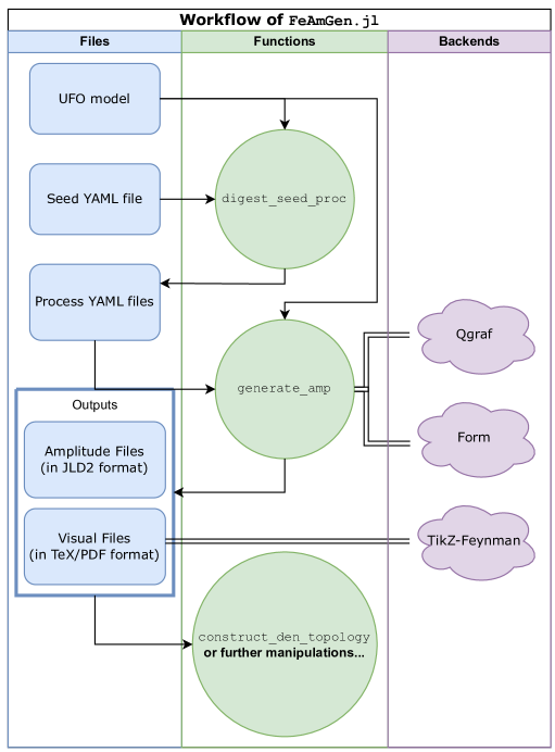
Figure 1: Workflow of FeAmGen.jl

2.1 Main functions

There are three functions exported for users:

1. digest_seed_proc( "/path/to/seed.yaml" ):
   The options defined in the seed YAML file will be checked, e.g., the lepton number violation and the quark generation violation. The partons will be expanded explicitly into several sub-processes, and the corresponding sub-process YAML files will be generated automatically, which contain all the information for generating the Feynman diagrams and the corresponding amplitudes.

2. generate_amp( "/path/to/process.yaml" ):
   This function will read in the process YAML file and the specified UFO model. Then it will generate all amplitudes files in the JLD2 format and their corresponding visual files as LaTeX files (TikZ-Feynman package is required for generating the corresponding PDF files). The human-readable text files (with the suffix out) will also be generated.

3. construct_den_topology( "/path/to/amplitude/directory/" ):
   Based on the amplitudes generated by the function generate_amp, users can utilize this function to construct the topologies that cover all Feynman amplitudes/integrals of the specified process.

In the following section, we will go into more detail about the usages of these functions. In particular, we have provided the sample scripts archived in test/ to demonstrate the usages of these functions as shown in Sec. 2.6. All the following sample codes have the assumption of using the package FeAmGen.jl via

⬇

using FeAmGen

2.2 Configuration files

Users need to prepare the UFO model and provide the information about the process to be generated. This information should be written in the YAML format, a human-friendly data serialization language. The seed YAML file will be detailed in the example gbtw_Test.jl for the process $gb\to tW^{-}$. The users are encouraged to copy it and make modifications as needed.

1 is the content of the seed YAML file for the process $gb\to tW^{-}$, which sets up 18 options in total. This configuration file in YAML format could be read by the functions digest_seed_proc and generate_amp. However, there are three options partons, AllowLeptonNumberViolation and AllowQuarkGenerationViolation that are only recognized by the function digest_seed_proc. Notice that the function generate_amp cannot resolve the "parton" in the incoming/outgoing particle list.

Listing 1: Simple YAML example of the process $gb\to tW^{-}$

⬇

model_name: "sm_CKMdiag_Haa"

unitary_gauge: true

# only for ‘digest_seed_proc‘

partons: ["g", "u", "ubar", "d", "dbar", "b", "bbar"]

AllowLeptonNumberViolation: false

AllowQuarkGenerationViolation: false

# only for ‘digest_seed_proc‘

DropTadpole: true

DropWFcorrection: true

n_loop: 2 # nloop

QCDCT_order: 0

Amp_QCD_order: 5 # 1 + 2 * nloop

Amp_QED_order: 1

Amp_SPC_order: 0

Amp_Min_Ep_Xpt: -4 # -2 * nloop

Amp_Max_Ep_Xpt: 0

incoming: ["b", "g"]

outgoing: ["Wminus", "t"]

momentum_symmetry: []

color_symmetry: []

All options in the YAML file are:

1. model_name: The name of the UFO model to invoke. It is worth mentioning that the function digest_seed_proc will search for the model files from the working directory if the location of the model file is missing.

2. unitary_gauge: (true/false) The option to choose the unitary gauge or not for the internal massive gauge bosons.

3. partons: (for digest_seed_proc only) The set of particles defined by the user can be used to generate the sub-processes. The users could use "parton" in the incoming/outgoing particle list instead of the specific particle name. Then the function digest_seed_proc will check this option and expand the "parton"’s into several sub-processes according to the particle list here.

4. AllowLeptonNumberViolation:(true/false, for digest_seed_proc only) The option for allowing/forbidding the violation of the lepton number.

5. AllowQuarkGenerationViolation: (true/false, for digest_seed_proc only) The option for allowing/forbidding the violation of the quark generation.

6. DropTadpole: (true/false) The option for dropping the diagrams with tadpoles or not (also known as the diagrams amputated or not).

7. DropWFcorrection: (true/false) The option for dropping the diagrams with corrections of wave functions or not.

8. n_loop: Number of loops.

9. QCDCT_order: Order of QCD counter terms. If the users want to generate order-$n_{\text{order}}$ with order-$n_{\text{CT}}$ Feynman diagrams/amplitudes, the entry n_loop should be set to $n_{\text{order}}-n_{\text{CT}}$ and the QCDCT_order should be set to $n_{\text{CT}}$.

10. Amp_QCD_order: Order of the QCD coupling in the amplitudes.

11. Amp_QED_order: Order of the QED coupling in the amplitudes.

12. Amp_SPC_order: Order of the special coupling in the amplitudes.
    The users could mark the special coupling order (SPC order) in the UFO model file for the vertices they are interested in. Then the users could specify the SPC order here for the diagram generation.

13. Amp_Min_Ep_Xpt: The minimal order of $\varepsilon$ in the series expansion of $\varepsilon$ in the amplitudes.

14. Amp_Max_Ep_Xpt: The maximal order of $\varepsilon$ in the series expansion of $\varepsilon$ in the amplitudes.

15. incoming: The set of incoming particles ("parton" is acceptable and it will be expanded by digest_seed_proc).

16. outgoing: The set of outgoing particles ("parton" is acceptable and it will be expanded by digest_seed_proc).

17. momentum_symmetry: Symmetries between external momenta. This option could be needed in the evaluation of cut diagrams. For instance, [K1, K3] means $K_{1}=K_{3}$, i.e., the replace $K_{3}\to K_{1}$ will be applied in the final expressions of the amplitudes.

18. color_symmetry: Symmetries between the colors carried by external particles. This option could be needed in the decay or scattering process of the bound state. For example, [1, 3] means the colors of particle 1 and particle 3 are the same, i.e. $\delta_{c_{1}c_{3}}$ will be inserted into the color factors and then calculated automatically.

With this seed YAML file, users could run the following code in the Julia REPL or script.

⬇

digest_seed_proc( "/path/to/seed.yaml" )

It will generate several process YAML files that archive the information of relevant sub-processes. The options partons, AllowLeptonNumberViolation and
AllowQuarkGenerationViolation will be checked. If the users want to generate diagrams and amplitudes for the process including "parton", e.g. $p+p\to t+\bar{t}$, the function digest_seed_proc will expand the partons and filter the sub-processes according the values of options AllowLeptonNumberViolation and AllowQuarkGenerationViolation. Please refer to the example of ppttbar_Test.jl for expanding partons in detail.

The process YAML file generated by digest_seed_proc with 1 as input will be saved in b_g_TO_Wminus_t_2Loop/b_g_TO_Wminus_t.yaml, where "b_g_TO_Wminus_t_2Loop" represents the process $gb\to tW^{-}$ at 2-loop obviously.

2.3 Generate amplitudes

There are several process YAML files generated by the function digest_seed_proc, which are almost structurally identical to the seed YAML file, except that they do not have the three options that will only be handled by the function digest_seed_proc and the entries "parton" in the incoming/outgoing particle list are expanded into partons explicitly. The users could further call the function generate_amp to generate all Feynman diagrams and the corresponding Feynman amplitudes as

⬇

generate_amp( "b_g_TO_Wminus_t_2Loop/b_g_TO_Wminus_t.yaml" )

Then two directories will be created: b_g_TO_Wminus_t_2Loop_amplitudes storing the amplitude files and b_g_TO_Wminus_t_2Loop_visuals storing the visualization files, respectively. Please refer to Sec. 2.7 for these two directories in detail.

The function generate_amp calls the external program Qgraf for generating the Feynman diagrams. The corresponding amplitudes will be constructed according to the generated diagrams and the information from the UFO model. The canonicalization will be applied to the amplitudes, which is explained in A. Then the amplitudes will be simplified by the computer algebra systems of SymEngine.jl and Form.

2.4 Construct complete topologies

FeAmGen.jl offers the function construct_den_topology for constructing the complete topologies. This function works in two modes:

1. Without momentum shift:

   ⬇

   construct_den_topology(

   "b_g_TO_Wminus_t_3Loop_amplitudes/";

   mom_shift_opt=false

   )

2. With momentum shift:

   • Without reference denominator topologies:

     ⬇

     construct_den_topology(

     "b_g_TO_Wminus_t_3Loop_amplitudes/";

     mom_shift_opt=true

     )

   • With reference denominator topologies:

     ⬇

     construct_den_topology(

     "b_g_TO_Wminus_t_3Loop_amplitudes/";

     mom_shift_opt=true,

     ref_dentop_collect=<base_top_dir>

     )

     where <base_top_dir> is the directory that archives the generated topologies for references. In this approach, the function construct_den_topology will read the topologies from the directory <base_top_dir> and then construct the topologies according to these topologies.

Then the complete set of topologies will be generated and saved in the topology directory (See Sec. 2.7.1 for more details). The algorithm for constructing Feynman integral topology is explained in B.

2.5 Model files

The Universal Feynman Output format [33], also known as Universal FeynRules Output format in its first version [34], is a model file format for several automatic matrix element generation software in high energy physics. The users could use the package FeynRules [36, 37] to generate the UFO models from the Lagrangian. The model files used in FeAmGen.jl are written in the UFO format, since it provides a flexible format archiving all the information about a theoretical model in an abstract form. Users can also specify the directory to search for the model files in the function digest_seed_proc as

⬇

digest_seed_proc( "/path/to/seed.yaml"; model_paths=[

"/path/to/the/first/model/directory",

"/path/to/the/second/model/directory"

] )

and in the function generate_amp as

⬇

generate_amp( "/path/to/seed.yaml"; model_paths=[

"/path/to/the/first/model/directory",

"/path/to/the/second/model/directory"

] )

In the UFO format, the information on the particles, parameters and vertices of the model are stored in a set of Python2 objects. For accessing the model files in FeAmGen.jl, PyCall.jl, the Julia interface to Python, is needed. Please refer to Sec. 3.3.2 for more details.

2.6 Run tests

We provide several tests in the directory FeAmGen.jl/test, which can be simply run by Pkg.jl as

⬇

using Pkg

Pkg.test("FeAmGen")

Details of every test are presented as follows.

2.6.1 Basic tests

The basic test file is basicTest.jl. Some key functions will be tested in this script. And users could report any bugs and make suggestions as Git issues${}^{\text{ or }}$.

2.6.2 Generic process generation

Generating all the Feynman diagrams and the corresponding amplitudes for the specific process is the most important feature of this package, which is covered in detail in the following test scripts.

1. ppttbar_Test.jl for $\text{p + p}\to t+\bar{t}$ at the tree and 1-loop levels;
   The incoming particles in this test are set to be "parton", which will be expanded by the function digest_seed_proc. In subsequent steps of this test, we will only generate the amplitudes and the visuals of the sub-process $gg\to t\bar{t}$ for simplicity.

2. DrellYan_Test.jl for $u\bar{d}\to W^{+}$ at tree, 1-loop and 2-loop level;

3. eeHZ_Test.jl for $e^{+}e^{-}\to HZ$ at tree and 1-loop level;

4. gbtw_Test.jl for $gb\to tW^{-}$ at tree, 1-loop and 2-loop level;

5. tWb_Test.jl for $t\to bW^{-}$ at 3-loop level;

6. tWtW_Test.jl for $tW^{+}\to tW^{+}$ at 3-loop level.

These tests will generate corresponding seed YAML files in the directory of test/ automatically. Then, FeAmGen.jl will read the seed YAML files and generate amplitudes and visuals for each process.

2.6.3 Construct complete top topologies

In this test, the complete topologies for the process $tW^{+}\to tW^{+}$ (at 2-loop and 3-loop) and the process $t\to t$ (at 4-loop) will be constructed. Before running this test, the results produced by tWb_Test.jl and tWtW_Test.jl must be prepared, which include the directories archiving the corresponding amplitudes in the JLD2 format. Please see Sec. 2.7.4 for more information about the constructed topologies.

2.7 Results

The results generated by FeAmGen.jl can be directly read by the subsequent programs we are developing. However, the users are also encouraged to utilize the results in their own way. We will demonstrate the details of the results generated by FeAmGen.jl in the process $tW^{+}\to tW^{+}$ at 3-loop as an example.

2.7.1 Directory tree structures

The generated files for $tW^{+}\to tW^{+}$ at 3-loop will be stored in the following structure.

• Wplus_t_TO_Wplus_t_2Loop/
  Main directory of $tW^{+}\to tW^{+}$ at 2-loop.

  • Wplus_t_TO_Wplus_t.yaml
    Process YAML file for $tW^{+}\to tW^{+}$ at 2-loop.

  • Wplus_t_TO_Wplus_t_2Loop_amplitudes/
    Amplitude directory.

    • amp1.jld2
      JLD2 file for amplitude.

    • …

    • amp1.out
      Human-readable file for amplitude.

    • …

  • Wplus_t_TO_Wplus_t_2Loop_shifted_amplitudes/
    Amplitude directory with momentum shift, which will be generated only if the option mom_shift_opt=true.

    • shifted_amp1.jld2
      JLD2 file for shifted amplitude.

    • …

  • Wplus_t_TO_Wplus_t_2Loop_shifted_topologies/
    Topology directory with momentum shift, which will be generated only if the option mom_shift_opt=true.

    • shifted_topology.out
      Human-readable file for topology.

    • topology1.jld2
      JLD2 file for topology.

    • …

  • Wplus_t_TO_Wplus_t_2Loop_topologies/
    Topology directory without momentum shift.

    • topology.out
      Human-readable file for topology.

    • topology1.jld2
      JLD2 file for topology.

    • …

  • Wplus_t_TO_Wplus_t_2Loop_visuals/
    Visual directory.

    • visual_diagram1.tex
      LaTeX file for plotting the Feynman diagram

    • …

    • expression_diagram1.out
      Human-readable file for amplitude

    • …

    • generate_diagram_pdf.jl
      Julia script for building all LaTeX files

The details of amplitudes, visuals, and topologies will be explained in the following sections.

2.7.2 Amplitudes

The most important part of the results generated by FeAmGen.jl is the Feynman amplitudes, which are archived in the directory <process>/<amplitude>, e.g. Wplus_t_TO_Wplus_t_2Loop/Wplus_t_TO_Wplus_t_2Loop_amplitudes. There are 2 types of files in the amplitude directory, the JLD2 files with suffix jld2 and the UTF-8 format text files with suffix out. The files with suffix out are the human-readable text files, which have the same information as the JLD2 files. FeAmGen.jl uses the JLD2 file format to archive the generated amplitudes. For reading it, JLD2.jl package is required, which is shown as

⬇

using JLD2

amp1 = load( "Wplus_t_TO_Wplus_t_2Loop/\

Wplus_t_TO_Wplus_t_2Loop_amplitudes/amp1.jld2" )

or

⬇

using JLD2

amp1 = jldopen( "Wplus_t_TO_Wplus_t_2Loop/\

Wplus_t_TO_Wplus_t_2Loop_amplitudes/amp1.jld2" )

<... The codes processing the amplitudes ...>

# One may need close(amp1) after all.

Then the variable amp1 will have type Dict (or type JLD2.JLDFile in the second case) in the Julia programming language. Users could access the amplitude information by amp1[<key>], where the <key> can be chosen as follows in this example.

• "Generator": Name of the generator.
  amp1["Generator"] == "FeAmGen.jl"

• "n_inc": Number of incoming particles.
  amp1["n_inc"] == 2

• "n_loop": Number of loops.
  amp1["n_loop"] == 2

• "min_ep_xpt": Minimal order of $\varepsilon$ in the series expansion of $\varepsilon$.
  amp1["min_ep_exp"] == -4

• "max_ep_xpt": Maximal order of $\varepsilon$ in the series expansion of $\varepsilon$.
  amp1["max_ep_exp"] == 0

• "couplingfactor": Coupling factor.
  amp1["couplingfactor"] == "1"

• "ext_mom_list": External momenta list.
  amp1["ext_mom_list"] == ["K1", "K2", "K3", "K4"]

• "scale2_list": List of mass squared scales.
  amp1["scale2_list"] == ["shat", "mw^2", "ver1", "mt^2"]

• "loop_den_list": List of denominators of the amplitudes.
  amp1["loop_den_list"] == String[...] with

  • "Den(q2, 0, 0)";

  • "Den(K3 - K1 - K2 + q1 + q2, 0, 0)";

  • "Den(K3 - K1 + q1, 0, 0,)";

  • "Den(q1, mt, 0)";

  • "Den(q1 + q2, mt, 0)",

  where "Den(P, m, ieta)" means $\quantity(P^{2}-m^{2}+\mathrm{i}\eta)^{-1}$. Notice that we adopt the conversions that K<i>’s(k<i>’s) and q<i>’s represent massive(massless) external momenta and loop momenta, respectively, where <i> is the integer index of the momenta.

• "loop_den_xpt_list": List of the exponents for the corresponding denominators.
  amp1["loop_den_xpt_list"] == [1, 1, 1, 1, 1]
  According to the information we have, the scalar integral should be

  $$I[1,1,1,1,1]=\int\quantity[\prod_{r=1}^{2}\frac{\differential^{D}q_{r}}{\mathrm{i}\pi^{D/2}}]\frac{1}{q_{2}^{2}\quantity(q_{12}+k_{123})^{2}\quantity(q_{1}+k_{13})^{2}\quantity(q_{1}^{2}-m_{t}^{2})\quantity(q_{12}^{2}-m_{t}^{2})},$$

  where $k_{123}:=-K_{1}-K_{2}+K_{3}$, $k_{13}:=-K_{1}+K_{3}$ and $q_{12}:=q_{1}+q_{2}$.

• "kin_relation": Dictionary of the kinematic relations.
  amp1["kin_relation"] == Dict{String, String}(...) with

  • "Den(K3 - K1, mt, 0)" => "ver2";

  • …

• "mom_symmetry": Symmetries between the external momenta.
  amp1["symmetry_map"] == Dict{String, String}().
  If not empty, e.g., Dict{"K1" => "K3"} means $K_{1}=K_{3}$.

• "color_symmetry": Symmetries between the external momenta.
  amp1["symmetry_map"] == Dict{Int, Int}().
  If not empty, e.g., Dict{1 => 3} means the colors of particle 1 and particle 3 are the same, i.e. $\delta_{c_{1}c_{3}}$ will be inserted into the color factors and then calculated automatically.

• "model_parameter_dict": Dictionary of model parameters.
  amp1["model_parameter_dict"] == Dict{String, String(…)} with

  • "sw" => "sqrt(sw2)";

  • …

• "model_coupling_dict": Dictionary of model couplings.
  amp1["model_coupling_dict"] == Dict{String, String(…)} with

  • "gcsub33" => "-6*im*lamh";

  • …

• "signed_symmetry_factor": Signed symmetry factor, the product relative sign from fermion line or loop and the symmetry factor of the Feynman diagram.
  amp1["signed_symmetry_factor"] == "1"

• "amp_color_list": List of color part expressions of the amplitude.
  amp1["amp_color_list] == String["..."]

• "amp_lorentz_list": List of Lorentz part expressions of the amplitude.
  amp1["amp_lorentz_list] == String["..."]

The users could read this information in the human-readable files with suffix out directly for convenience, and it is preferred to read JLD2 files in the programs.

2.7.3 Visuals

The visualization of Feynman diagrams could be helpful for the users to understand the interaction mechanism. Therefore, all visual files are provided in the directory <process>/<visual>, e.g. Wplus_t_TO_Wplus_t_2Loop/Wplus_t_TO_Wplus_t_2Loop_visuals for $tW^{+}\to tW^{+}$ at 2-loop. There are also two types of files in the visual directory, which are LaTeX files with suffix tex and the UTF-8 text files with suffix out. The files with suffix out are also the human-readable text files, which archive the information of

• Loop denominators;

• Loop denominator powers;

• Coupling factor;

• Symmetry of external momenta;

• List of color factors;

• List of Lorentz part factors of the amplitude.

Please refer to Sec. 2.7.2 for more information about the above entries.

The LaTeX files with suffix tex should be compiled via lualatex for the TikZ-Feynman LaTeX package. We also provide the Julia script generate_diagram_pdf.jl in every visual directory to compile these files in batch (see Sec. 2.7.1 for details). The first Feynman diagram generated by FeAmGen.jl for $tW^{+}\to tW^{+}$ at 2-loop is shown as Fig. 2.

Figure 2: Diagram 1 (Sign: 1, Symmetry factor: 1) for $tW^{+}\to tW^{+}$ at 2 loop

2.7.4 Topologies

The topology information is archived in the directory <process>/<topology>, which archives a human-readable file named (shifted_)topology.out in the UTF-8 format. Also, the separate JLD2 files archive relevant single topology. As an example, the first topology constructed for $tW^{+}\to tW^{+}$ at 2-loop with momentum shift contains the following information.

• The amplitude files covered by this topology:

  • /path/to/amp11.jld2

  • /path/to/amp7.jld2 with momentum shift:

    • $q_{1}\to-q_{1}-K_{3}$

    • $q_{2}\to-q_{2}$

  • /path/to/amp29.jld2

  • /path/to/amp157.jld2

• Denominators of this topology

  • Den(K3 - K1 + q1, 0, 0)

  • Den(K3 - K1 - K2 + q1 + q2, 0, 0)

  • Den(q1, mt, 0)

  • Den(K3 + q1, 0, 0)

  • Den(q2, 0, 0)

  • Den(q1 + q2, mt, 0)

  • Den(K1 + q2, mt, 0)

  • Den(K2 + q2, 0, 0)

By including the momentum shifts, we can construct 45 topologies to cover the 281 amplitudes of $tW^{+}\to tW^{+}$ at 2-loop.

3 Installation

Within the Julia ecosystem, the users could just use the package manager Pkg.jl to install the FeAmGen.jl. Julia v1.6 or later is required. We recommend the Linux platform for FeAmGen.jl. However, MacOS is also supported by the Julia ecosystem.

3.1 Install Julia

The ecosystem Julia can be installed whether using precompiled binaries or compiling from source by following the instructions at https://julialang.org/downloads directly.

3.2 Install External Programs

FeAmGen.jl needs external programs of Form and Qgraf as back-ends. Please refer to the following paragraphs for their installations.

Install QGRAF (v3.6.5)

Qgraf is a computer program written in Fortran, which could generate Feynman diagrams for various types of QFT models. FeAmGen.jl will download Qgraf from http://cfif.ist.utl.pt/~paulo/d.html and build it automatically if the Fortran compiler is provided by ENV["FC"] = "/path/to/fortran. The users should agree with the license of Qgraf before using this package. The users can set this variable in the Julia startup file, which archives the codes that you want executed whenever Julia is run. FeAmGen.jl will also check the variable ENV["QGRAF"] for the path to the Qgraf installed in your computer. Therefore, the user should add ENV["QGRAF"] = "/path/to/qgraf" into the Julia startup file.

Install FORM (v4.3.1)

Form is designed for the symbolic manipulation of big expressions. Please visit the home page of Form for more information and installation instructions. Also FeAmGen.jl can automatically invoke the binary interface for Form provided by the Julia package FORM_jll.jl on platforms other than Windows. For Windows users, we recommend using the Windows Subsystem for Linux 2 (WSL2), which provides a Linux virtual machine but with the performance comparable to the physical machine.

3.3 Install Julia Packages

Most of Julia packages required by FeAmGen.jl are managed by the Pkg.jl, which is the package management for Julia programming language. Therefore, they could be installed automatically when you install FeAmGen.jl.

3.3.1 Add Registry IHEP-Multiloop

Julia registries contain information about packages, such as available releases and dependencies, and where they can be downloaded. The General registry is the default registry. The IHEP-Multiloop registry is the Julia registry maintained by the authors, which provides the information about the package FeAmGen.jl and its dependencies developed and maintained by the authors.

⬇

using Pkg

Pkg.Registry.add("General")

Pkg.Registry.add( Pkg.Registry.RegistrySpec( url=

"https://code.ihep.ac.cn/IHEP-Multiloop/JuliaRegistry")

)

3.3.2 Addtional information about PyCall.jl

The UFO format is written in the Python programming language. Therefore, the Julia package PyCall.jl is used in FeAmGen.jl to read the model files in the UFO format. However, the UFO formats exported from the latest version of FeynRules are still written in Python2, which had been stopped by Python developers in 2020. Fortunately, PyCall.jl supports calling Python2 directly right now. Hence, there are two approaches to reading UFO format in FeAmGen.jl:

1. Build the PyCall.jl with Python2.7;

2. Convert the UFO formats from Python2 to Python3.

The first is more cumbersome and it will not be presented here. Users can consult the documentation of PyCall.jl for more details. We recommend the second approach. The conversion can be done directly by the tool script 2to3 provided by Python3.

3.4 Install FeAmGen.jl

After adding the IHEP-Multiloop registry, users may install FeAmGen.jl by running

⬇

using Pkg

Pkg.add("FeAmGen")

All other Julia dependencies are installed automatically during the installation procedure.

4 Conclusion

In this paper, we present the Julia package FeAmGen.jl, a powerful and versatile Julia program that can handle the challenging task of generating and calculating Feynman diagrams and amplitudes for various quantum field theory processes. The program is designed to meet the increasing demand for high precision theoretical predictions in particle physics, especially in the era of precise tests of the Standard Model and beyond. The program takes advantage of the UFO model format, which allows users to define arbitrary models and couplings conveniently. The program also relies on Qgraf and Form, the well-established external tools that can efficiently generate Feynman diagrams and simplify amplitude expressions. Moreover, the program provides useful functions to construct topologies that cover all possible Feynman integrals of a given process at any loop level, and to produce visual files for the diagrams via TikZ-Feynman, a LaTeX package that can create beautiful and clear diagrams.

In this paper, we give a detailed description of the main functions and workflow of the program, as well as the installation instructions and test examples. The paper also showcases some applications of the program for generating process amplitudes at different loop levels, with examples ranging from Drell-Yan process to top quark decay.

Note Added: This package has recently had some applications for SMEFT one-loop matching, for which we are working on a tiny derivative of this package.

Appendices

Appendix A Canonicalization of Feynman Integrals

A.1 Canonical Form of Feynman Integrals

The general form of the Feynman integral is given as (for $n_{\text{ext}}$ external legs, $n_{\text{int}}$ propagators, $\ell$ loops and $D$ space-time dimensions)

$$I=\int\quantity[\prod_{r=1}^{\ell}\frac{\differential^{D}q_{r}}{\mathrm{i}\pi^{D/2}}]\prod_{j=1}^{n_{\text{int}}}\frac{1}{\quantity(P_{j}^{2}-m_{j}^{2}+\mathrm{i}\eta)^{\nu_{j}}},$$ (1)

where

$$P_{j}=\sum_{r=1}^{\ell}\lambda_{jr}q_{r}+\sum_{r=1}^{n_{\mathrm{ext}}-1}\sigma_{jr}k_{r}.$$ (2)

Here $\quantity{q_{r}}_{r=1}^{\ell}$ is the set of loop momenta and $\quantity{k_{r}}_{r=1}^{n_{\mathrm{ext}}}$ is the set of external momenta, which is assumed to be linearly independent. There are $n_{\text{int}}$ propagators with momenta $\quantity{P_{j}}_{j=1}^{\ell}$ and masses $\quantity{m_{j}}_{j=1}^{n_{\text{int}}}$. The coefficients $\lambda_{jr}$’s and $\sigma_{jr}$’s are determined by the momentum conservation and the momentum symmetry.

Figure 1: A simple example of 2-loop Feynman diagram. $K_{j}$’s for massive external momenta and $k_{j}$’s for massless external momenta. The thick lines represent the massive propagators and massive external particles with mass $m$, i.e., $K_{j}^{2}=m^{2}$ here.

For example, the 2-loop Feynman integral of Fig. 1 is given as

$$I_{2}=\int\frac{\differential[D]{q_{1}}}{\mathrm{i}\pi^{D/2}}\frac{\differential[D]{q_{2}}}{\mathrm{i}\pi^{D/2}}\frac{1}{\mathcal{D}_{1}\mathcal{D}_{2}\cdots\mathcal{D}_{7}},$$ (3)

where

$$\mathcal{D}_{1} =q_{1}^{2}+\mathrm{i}\eta,$$ (4)

$$\mathcal{D}_{2} =q_{2}^{2}+\mathrm{i}\eta,$$ (5)

$$\mathcal{D}_{3} =(q_{1}+K_{2})^{2}-m^{2}+\mathrm{i}\eta,$$ (6)

$$\mathcal{D}_{4} =(q_{1}-k_{1})^{2}+\mathrm{i}\eta,$$ (7)

$$\mathcal{D}_{5} =(q_{2}+K_{3})^{2}-m^{2}+\mathrm{i}\eta,$$ (8)

$$\mathcal{D}_{6} =(q_{1}-q_{2}-k_{1})^{2}+\mathrm{i}\eta,$$ (9)

$$\mathcal{D}_{7} =(q_{1}-q_{2}+K_{2}-K_{3})^{2}+\mathrm{i}\eta.$$ (10)

However, this form is not unique. The momentum shift

$$\left\{\begin{aligned} q_{1}&\to q_{1}^{\prime}+k_{1}\\ q_{2}&\to q_{1}^{\prime}+q_{2}^{\prime}-k_{1}\end{aligned}\right.$$ (11)

could be applied to the above integral, and the new integral is given as

$$I_{2}^{\prime}=\int\frac{\differential[D]{q_{1}^{\prime}}}{\mathrm{i}\pi^{D/2}}\frac{\differential[D]{q_{2}^{\prime}}}{\mathrm{i}\pi^{D/2}}\frac{1}{\mathcal{D}_{1}^{\prime}\mathcal{D}_{2}^{\prime}\cdots\mathcal{D}_{7}^{\prime}},$$ (12)

where

$$\mathcal{D}_{1}^{\prime} =(q_{1}^{\prime}+k_{1})^{2}+\mathrm{i}\eta,$$ (13)

$$\mathcal{D}_{2}^{\prime} =(q_{1}^{\prime}+q_{2}^{\prime}-k_{1})^{2}+\mathrm{i}\eta,$$ (14)

$$\mathcal{D}_{3}^{\prime} =(q_{1}^{\prime}+k_{1}+K_{2})^{2}-m^{2}+\mathrm{i}\eta,$$ (15)

$$\mathcal{D}_{4}^{\prime} =q_{1}^{\prime 2}+\mathrm{i}\eta,$$ (16)

$$\mathcal{D}_{5}^{\prime} =(q_{1}^{\prime}+q_{2}^{\prime}-k_{1}+K_{3})^{2}-m^{2}+\mathrm{i}\eta,$$ (17)

$$\mathcal{D}_{6}^{\prime} =(q_{2}^{\prime}-k_{1})^{2}+\mathrm{i}\eta,$$ (18)

$$\mathcal{D}_{7}^{\prime} =(q_{1}^{\prime}-2k_{1}+K_{2}-K_{3})^{2}+\mathrm{i}\eta.$$ (19)

Obviously, $I_{2}\equiv I_{2}^{\prime}$. The momentum shift, however, introduces redundancy in the description of the Feynman Integrals, which hinders our handling of the Feynman integrals, e.g. the integral-by-part (IBP) reduction.

The redundancy can be removed by the canonicalization of the Feynman integrals, i.e., we choose the unique form from the equivalent Feynman integrals to represent all of them. The unique form is called the canonical form in the following discussions. The requirements that the canonical form of the Feynman integral in the FeAmGen.jl should meet are shown as follows:

1. The coefficients in Eq. 2 should satisfy

   $$\lambda_{jr}=\left\{\begin{matrix}\delta_{jr}&j\leq\ell,\\ 0\text{ or }1&j>\ell,\end{matrix}\right.\mbox{\quad and\quad}\sigma_{jr}=\left\{\begin{matrix}0&j\leq\ell,\\ 0\text{ or }\pm 1&j>\ell.\end{matrix}\right.$$ (20)

2. The relevant vacuum integral for the Feynman integral Eq. 1 could be expressed as

   $$I_{\text{vac}}\sim\int\quantity[\prod_{r=1}^{\ell}\frac{\differential^{D}q_{r}}{\mathrm{i}\pi^{D/2}}]\prod_{j=1}^{n_{\text{int}}}\frac{1}{\quantity(P_{j,\mathrm{vac}}^{2}-m_{j}^{2}+\mathrm{i}\eta)^{\nu_{j}}},$$ (21)

   where

   $$P_{j,\mathrm{vac}}=\sum_{r=1}^{\ell}\lambda_{jr}q_{r}.$$ (22)

   In the cases of up to 4 loops, the vacuum momenta $\quantity{P_{j,\mathrm{vac}}}_{j=1}^{n_{\mathrm{int}}}$ of the canonical form of the Feynman integral should be the subset of any of the following sets:

   • 1-loop: $\quantity{q_{1}}$;

   • 2-loop: $\quantity{q_{1},q_{2},q_{1}+q_{2}}$;

   • 3-loop:

     • $\quantity{q_{1},q_{2},q_{3},q_{1}+q_{3},q_{2}+q_{3},q_{1}+q_{2}+q_{3}}$;

     • $\quantity{q_{1},q_{2},q_{3},q_{1}+q_{2},q_{1}+q_{3},q_{2}+q_{3}}$;

   • 4-loop:

     • $\{q_{1},q_{2},q_{3},q_{4},q_{1}+q_{2},q_{1}+q_{3},q_{2}+q_{4},q_{1}+q_{2}+q_{3},q_{1}+q_{2}+q_{4},q_{1}+q_{2}+q_{3}+q_{4}\}$;

     • $\{q_{1},q_{2},q_{3},q_{4},q_{1}+q_{2},q_{1}+q_{3},q_{2}+q_{4},q_{3}+q_{4},q_{2}+q_{3}+q_{4},q_{1}+q_{2}+q_{3}+q_{4}\}$;

     • $\{q_{1},q_{2},q_{3},q_{4},q_{1}+q_{2},q_{1}+q_{3},q_{2}+q_{3},q_{2}+q_{4},q_{1}+q_{2}+q_{4},q_{2}+q_{3}+q_{4}\}$.

3. In the propagator momenta $P_{j}$’s, the coefficients of the loop momenta $q$’s and external momenta $k$’s (for massless particles and $K$’s for massive particles) should be $0$ or $\pm 1$.

Although these three requirements can filter out most of the momentum shifts, there are still a large number of possibilities that will not be removed. We will define an order to sort all remaining possible forms of the Feynman integrals and define the one with the smallest order as the canonical form. In the next sub-section, we will describe the algorithm of canonicalization in detail.

A.2 Canonicalization Algorithm

The first part of the canonicalization algorithm is to find the possible momentum shifts that can be applied to the Feynman integral. It is important to note that the momentum shift is a transformation of the loop momenta, which are the direct integration variables of the Feynman integral. After such a momentum shift, we hope that the general form of Feynman integral of Eq. 1 should be preserved, which requires

$$\absolutevalue{\det T}\equiv 1,$$ (23)

where $T$ is the transformation matrix of the momentum shift, i.e., $q\to q^{\prime}=Tq$. For simplicity, we only consider the momentum shift that could be derived from the original Feynman diagrams.

Figure 2: Internal graph of Fig. 1, where the number $i$ label the vertex connecting the $i$-th external leg that has been removed.

Firstly, we consider the momenta shift without external momenta. We introduce the internal graph $G_{\text{int}}$ associated to the Feynman diagram, which is obtained by removing all external legs but preserving the vertices connecting external legs from the Feynman diagram. For example, the internal graph of Fig. 1 is shown in Fig. 2. If the external momenta are set to 0, there are only three unique propagator momenta in this internal graph, e.g., $\quantity{q_{1},q_{2},q_{1}\pm q_{2}}$. One could choose any two propagators from the internal graph, and make their propagator momenta as $\pm\tilde{q}_{1}$ or $\pm\tilde{q}_{2}$. If the chosen propagators are valid, i.e., the corresponding propagator momenta are linearly independent, then the momentum shift could be calculated by solving the linear equations $\tilde{q}=\tilde{T}q$, where $\tilde{T}_{im}=\pm\lambda_{jm}$. Here $j$ is the chosen propagator index, and $i$ is the shifted loop momentum index. The momentum shift without external momenta is simply given as $q\to\tilde{T}^{-1}\tilde{q}$.

The external momenta are then considered. Following the same procedure, we could choose any two propagators from the original graph, and make their propagator momenta as $\pm q_{1}^{\prime}$ or $\pm q_{2}^{\prime}$. Obviously,

$$q_{i}^{\prime}=\tilde{q}_{i}\pm\sum_{m=1}^{n_{\mathrm{ext}}-1}\sigma_{jm}k_{m},$$ (24)

where $\tilde{q}_{i}$’s are the corresponding shifted loop momenta without the consideration of external momenta. Then,

$$q_{i}^{\prime}\mp\sum_{m=1}^{n_{\mathrm{ext}}-1}\sigma_{jm}k_{m}=\quantity(\tilde{T}q)_{i}.$$ (25)

Finally, we have the momentum shift with external momenta as

$$q\to\tilde{T}^{-1}\quantity(q^{\prime}\mp\sigma\cdot k).$$ (26)

The algorithm will search all possible momentum shifts that could be derived from the original Feynman diagrams as described above. Then, the requirements of the canonical form of the Feynman integrals will be checked. However, an enormous number of possible momentum shifts are still allowed. We propose an order to sort all possible shifted propagator momenta, and the leading one will be chosen as the canonical form. The order is defined as a two-entry tuple of integers. Considering the case with 3 loops and 4 external legs (3 independent external momenta), the first entry is calculated by the following steps

1. For every propagator momentum, the normalization should be applied. This means that the coefficient of the first loop momentum $q_{i}$ with a non-zero coefficient in the propagator momenta should be normalized to $+1$, where the first means the smallest index of the loop momenta. For instance, $-q_{2}+q_{3}-K_{1}+k_{2}$ should be normalized to $q_{2}-q_{3}+K_{1}-k_{2}$.

2. Because of the second and the third requirements of the canonical form, the coefficients of all loop momenta and external momenta are either $0$ or $\pm 1$. For every propagator momentum, we could calculate the coefficients of all loop momenta and external momenta. For instance, the coefficients of normalized propagator momentum $q_{2}-q_{3}+K_{1}-k_{2}$ are

   $$\begin{matrix}k_{3}&k_{2}&K_{1}&q_{3}&q_{2}&q_{1}\\ 0&-1&+1&-1&+1&0\\ 0&2&1&2&1&0\end{matrix}$$ (27)

   where we substitute $-1$ with $2$ in the last line. Now the the digit sequence of the coefficients of all loop momenta and external momenta is obtained as $021210$, which could be converted to a ternary number $(21210)_{3}=(210)_{10}$, which is called propagator momentum number here.

3. Finally, the first entry of the order is the product of the propagator momentum numbers of all propagator momenta.

The second entry is the SHA-256 number calculated from the string of the list of the propagator momenta where the propagator momenta is sorted by lexicographical order.

Thus, the canonical form of the Feynman integral is obtained.

Appendix B Feynman Integral Topology

For a general form of scalar Feynman integral of

$$I[\nu_{1}\nu_{2}\cdots\nu_{\text{int}}]=\int\quantity[\prod_{r=1}^{\ell}\frac{\differential^{D}q_{r}}{\mathrm{i}\pi^{D/2}}]\prod_{j=1}^{n_{\text{int}}}\frac{1}{\quantity(P_{j}^{2}-m_{j}^{2}+\mathrm{i}\eta)^{\nu_{j}}},$$ (28)

where $\nu_{i}\in\mathbb{Z}$. We call the set of $n_{\text{int}}$ denominators $\{P_{j}^{2}-m_{j}^{2}+\mathrm{i}\eta\}_{j=1}^{n_{\text{int}}}$ as the topology of this scalar Feynman integrals. There are, however, $N_{V}$($\equiv(\ell+1)\ell/2+\ell(n_{\text{ext}}-1)$) independent scalar products (ISP) of loop momenta and external momenta for $\ell$-loop $n_{\text{ext}}$-leg Feynman diagrams. If $n_{\text{int}}<N_{V}$ or not all ISPs can be represented as the linear combination of all the inverses of propagators, some additional propagators should be added to make the topology complete. [28]

The well-known algorithm to solve this problem is the Pak’s algorithm [38] and its derivations [39, 40]. Instead of Pak’s algorithm, FeAmGen.jl apply another algorithm similar to the algorithm of canonicalization of Feynman integrals which is described in A for constructing the topology of Feynman integrals. The algorithm is described as follows.

1. Without momentum shift: In this approach, FeAmGe.jl do not consider the momentum shift. Then the function construct_den_topology will construct the minimum topology that can cover as many as Feynman diagrams as possible. Finally, the generated topologies will be completed.

2. With mometnum shift:

   • Without reference denominator topologies: In this way, the reference denominator topologies is set to be empty. Then the first denominator topology will be added into the reference denominator topologies. For the rest denominator topologies, we will search the momentum shift that can make the denominator topology covered by the reference denominator topologies or covering one of the reference denominator topologies. If the momentum shift is found, the shifted denominator topology will be chosen and added into the reference denominator topologies. Otherwise, the original denominator topology will be added into the reference denominator topologies directly. Finally, all of chosen denominator topologies will be completed.

   • With reference denominator topologies: In this approach, the reference denominator topologies is given. The rest is the same as the previous approach.

To complete the topology, some additional propagators should be added to the denominator topologies. The additional propagators are constructed from the linear combination of loop mometna in the second requirement for canonical form of Feynman integrals, which is described in A. For example, we consider the independent external momenta $K_{\mathrm{ext}}=\quantity{K_{1},k_{2},k_{3}}$ and the propagator momenta is a subset of the first case in the 3-loop, i.e. a subset of $Q_{\mathrm{int}}=\quantity{q_{1},q_{2},q_{3},q_{1}+q_{3},q_{2}+q_{3},q_{1}+q_{2}+q_{3}}$. Then, the ISPs in $\quantity{\quantity(Q\pm K)^{2}\middle|Q\in Q_{\mathrm{int}}\wedge K\in K_{\mathrm{ext}}}$ will be checked whether they can be represented as the linear combination of all the inverses of propagators. If not, the additional propagators will be added to the denominator topologies.

Finally, the complete topologies are constructed.

References

- [1] M. E. Peskin, D. V. Schroeder, An Introduction to Quantum Field Theory, Addison-Wesley Pub. Co., Reading, USA, 1995.
- [2] M. Veltman, Diagrammatica, 1st Edition, Cambridge University Press, 1994. doi:10.1017/CBO9780511564079.
- [3] J. Butler, R. Chivukula, A. de Gouvea, et al., Report of the 2021 U.S. Community Study on the Future of Particle Physics Snowmass 2021, in: Snowmass, Seattle, WA (United States), September 2021, US DOE, 2023. doi:10.2172/1922503.
- [4] Particle Data Group, Review of Particle Physics, Prog. Theo. and Exp. Phys. 2022 (8) (aug 2022). doi:10.1093/ptep/ptac097.
- [5] The CMS Collaboration, Observation of a New Boson at a Mass of 125 GeV with the CMS Experiment at the LHC, Phys. Lett. B 716 (1) (2012) 30–61. arXiv:1207.7235, doi:10.1016/j.physletb.2012.08.021.
- [6] The ATLAS Collaboration, Observation of a New Particle in the Search for the Standard Model Higgs Boson with the ATLAS Detector at the LHC, Phys. Lett. B 716 (1) (2012) 1–29. doi:10.1016/j.physletb.2012.08.020.
- [7] G. Apollinari, O. Brüning, T. Nakamoto, L. Rossi, High Luminosity Large Hadron Collider HL-LHC, CERN Yellow Rep. (5) (2015) 1–19. arXiv:1705.08830, doi:10.5170/CERN-2015-005.1.
- [8] The International Linear Collider Technical Design Report - Volume 2: Physics (6 2013). arXiv:1306.6352.
- [9] The International Linear Collider Technical Design Report - Volume 1: Executive Summary (6 2013). arXiv:1306.6327.
- [10] P. Bambade, et al., The International Linear Collider: A Global Project (3 2019). arXiv:1903.01629.
- [11] M. Dong, et al., CEPC Conceptual Design Report: Volume 2 - Physics & Detector (11 2018). arXiv:1811.10545.
- [12] CEPC Conceptual Design Report: Volume 1 - Accelerator (9 2018). arXiv:1809.00285.
- [13] M. Bicer, et al., First Look at the Physics Case of TLEP, JHEP 01 (2014) 164. arXiv:1308.6176, doi:10.1007/JHEP01(2014)164.
- [14] A. Abada, et al., FCC Physics Opportunities: Future Circular Collider Conceptual Design Report Volume 1, Eur. Phys. J. C 79 (6) (2019) 474. doi:10.1140/epjc/s10052-019-6904-3.
- [15] A. Abada, et al., FCC-ee: The Lepton Collider: Future Circular Collider Conceptual Design Report Volume 2, Eur. Phys. J. ST 228 (2) (2019) 261–623. doi:10.1140/epjst/e2019-900045-4.
- [16] The CEPC Study Group, CEPC Conceptual Design Report: Volume 1 – Accelerator (Sep. 2018). arXiv:1809.00285.
- [17] The CEPC Study Group, CEPC Conceptual Design Report: Volume 2 – Physics & Detector (Nov. 2018). arXiv:1811.10545.
- [18] The FCC Collaboration, FCC-ee: The Lepton Collider: Future Circular Collider Conceptual Design Report Volume 2, Eur. Phys. J. Special Topics 228 (2) (2019) 261–623. doi:10.1140/epjst/e2019-900045-4.
- [19] The FCC Collaboration, FCC-hh: The Hadron Collider: Future Circular Collider Conceptual Design Report Volume 3, Eur. Phys. J. Special Topics 228 (4) (2019) 755–1107. doi:10.1140/epjst/e2019-900087-0.
- [20] The FCC Collaboration, FCC Physics Opportunities: Future Circular Collider Conceptual Design Report Volume 1, Eur. Phys. J. C 79 (6) (jun 2019). doi:10.1140/epjc/s10052-019-6904-3.
- [21] E. Ploerer, QCD at the Future Circular Collider (Aug. 2022). arXiv:2208.08250.
- [22] The ILC Collaboration, The International Linear Collider: Report to Snowmass 2021 (Mar. 2022). arXiv:2203.07622.
- [23] The ILC Collaboration, The International Linear Collider Technical Design Report – Volume 2: Physics (Jun. 2013). arXiv:1306.6352.
- [24] X. Liu, Y.-Q. Ma, AMFlow: A Mathematica Package for Feynman Integrals Computation via Auxiliary Mass Flow, Comput. Phys. Commun. 283 (2023) 108565. arXiv:2201.11669, doi:10.1016/j.cpc.2022.108565.
- [25] P. Nogueira, Automatic Feynman Graph Generation, J. Comput. Phys. 105 (2) (1993) 279–289. doi:10.1006/jcph.1993.1074.
- [26] Z. Li, Y. Wang, Q.-f. Wu, Categorization of Two-loop Feynman Diagrams in the Correction to , Chin. Phys. C 45 (5) (2021) 053102. arXiv:2012.12513, doi:10.1088/1674-1137/abe84d.
- [27] J. Küblbeck, M. Böhm, A. Denner, Feyn arts – Computer-algebraic Generation of Feynman Graphs and Amplitudes, Comput. Phys. Commun. 60 (2) (1990) 165–180. doi:10.1016/0010-4655(90)90001-H.
- [28] S. Weinzierl, Feynman Integrals, Springer International Publishing, 2022. arXiv:2201.03593, doi:10.1007/978-3-030-99558-4.
- [29] T. Hahn, Generating Feynman Diagrams and Amplitudes with FeynArts 3, Comput. Phys. Commun. 140 (3) (2001) 418–431. arXiv:hep-ph/0012260, doi:10.1016/S0010-4655(01)00290-9.
- [30] R. Mertig, M. Böhm, A. Denner, Feyn Calc – Computer-Algebraic Calculation of Feynman Amplitudes, Comput. Phys. Commun. 64 (3) (1991) 345–359. doi:10.1016/0010-4655(91)90130-D.
- [31] V. Shtabovenko, R. Mertig, F. Orellana, New Developments in FeynCalc 9.0, Comput. Phys. Commun. 207 (2016) 432–444. arXiv:1601.01167, doi:10.1016/j.cpc.2016.06.008.
- [32] V. Shtabovenko, R. Mertig, F. Orellana, FeynCalc 9.3: New features and improvements, Comput. Phys. Commun. 256 (2020) 107478. arXiv:2001.04407, doi:10.1016/j.cpc.2020.107478.
- [33] L. Darmé, C. Degrande, C. Duhr, et al., UFO 2.0 – The Universal Feynman Output format (Apr. 2023). arXiv:2304.09883.
- [34] C. Degrande, C. Duhr, B. Fuks, et al., UFO –The Universal FeynRules Output, Comput. Phys. Commun. 183 (6) (2012) 1201–1214. doi:10.1016/j.cpc.2012.01.022.
- [35] J. P. Ellis, TikZ-Feynman: Feynman diagrams with TikZ, Comput. Phys. Commun. 210 (2017) 103–123. doi:10.1016/j.cpc.2016.08.019.
- [36] A. Alloul, N. D. Christensen, C. Degrande, C. Duhr, B. Fuks, FeynRules 2.0 – A Complete Toolbox for Tree-level Phenomenology, Comput. Phys. Commun. 185 (8) (2013) 2250–2300. arXiv:1310.1921, doi:10.1016/j.cpc.2014.04.012.
- [37] N. D. Christensen, C. Duhr, FeynRules – Feynman Rules Made Easy, Comput. Phys. Commun. 180 (9) (2008) 1614–1641. arXiv:0806.4194, doi:10.1016/j.cpc.2009.02.018.
- [38] A. Pak, The Toolbox of modern multi-loop calculations: novel analytic and semi-analytic techniques, J. Phys. Conf. Ser. 368 (2012) 012049. arXiv:1111.0868, doi:10.1088/1742-6596/368/1/012049.
- [39] V. Shtabovenko, FeynCalc goes multiloop, J. Phys. Conf. Ser. 2438 (1) (2023) 012140. arXiv:2112.14132, doi:10.1088/1742-6596/2438/1/012140.
- [40] Z. Wu, J. Boehm, R. Ma, H. Xu, Y. Zhang, NeatIBP 1.0, A package generating small-size integration-by-parts relations for Feynman integrals (5 2023). arXiv:2305.08783.