Differentiable Euler Characteristic Transforms for Shape Classification

Abstract

The Euler Characteristic Transform (ECT) has proven to be a powerful representation, combining geometrical and topological characteristics of shapes and graphs. However, the ECT was hitherto unable to learn task-specific representations. We overcome this issue and develop a novel computational layer that enables learning the ECT in an end-to-end fashion. Our method DECT is fast and computationally efficient, while exhibiting performance on a par with more complex models in both graph and point cloud classification tasks. Moreover, we show that this seemingly unexpressive statistic still provides the same topological expressivity as more complex topological deep learning layers provide.

1 Introduction

Geometrical and topological characteristics play an integral role in the classification of complex shapes. Regardless of whether they are represented as point clouds, meshes (simplicial complexes), or graphs, a multi-scale perspective provided by methods from topological data analysis (TDA) can be applied for classification tasks. Of particular relevance in this context are the Persistent Homology Transform (PHT) and the Euler Characteristic Transform (ECT). Originally introduced by Turner et al. [36], recent work proved under which conditions both transforms are invertible, thus constituting an injective map [13, 7]. Both transforms are based on the idea of looking at a shape from multiple directions, and evaluating a multi-scale topological descriptor for each such direction. For the PHT, this descriptor is persistent homology, a method for assigning multi-scale topological features to input data, whereas for the ECT, the descriptor consists of the Euler characteristic, an alternating sum of elements of a space. The collection of all these direction–descriptor pairs is then used to provide a classification or solve an optimisation task. This approach is mathematically sound, but evaluating all possible directions is infeasible in practice, thus posing a severe limitation of the applicability of the method.

Our contributions.

We overcome the computational limitations and present a differentiable, end-to-end-trainable Euler Characteristic Transform. Our method (i) is highly scalable, (ii) affords an integration into deep neural networks (as a layer or loss term), and (iii) exhibits advantageous performance in different shape classification task for various modalities, including graphs, point clouds, and meshes.

2 Related Work

We first provide a brief overview of topological data analysis (TDA) before discussing alternative approaches for shape classification. TDA aims to apply tools from algebraic topology to data science questions; this is typically accomplished by computing algebraic invariants that characterise the connectivity of data. The flagship algorithm of TDA is persistent homology (PH), which extracts multi-scale connectivity information about connected components, loops, and voids from point clouds, graphs, and other data types [2, 11]. It is specifically advantageous because of its robustness properties [34], providing a rigorous approach towards analysing high-dimensional data. PH has thus been instrumental for shape analysis and classification, both with kernel-based methods [33] and with deep neural networks [20]. Recent work even showed that despite its seemingly discrete formulation, PH is differentiable under mild conditions [28, 5, 21, 22], thus permitting integrations into standard machine learning workflows. Of particular relevance for shape analysis is the work by Turner et al. [36], which showed that a transformation based on PH provides an injective characterisation of shapes. This transformation, like PH itself, suffers from computational limitations that preclude its application to large-scale data sets. As a seemingly less expressive alternative, Turner et al. [36] thus introduced the Euler Characteristic Transform (ECT), which is highly efficient and has proven its utility in subsequent applications [1, 7, 27, 30]. It turns out that despite its apparent simplicity, the ECT is also injective, thus theoretically providing an efficient way to characterise shapes [13]. A gainful use in the context of deep learning was not attempted so far, however, with the ECT and its variants [24, 26] still being used as static feature descriptors that require domain-specific hyperparameter choices. By contrast, our approach makes the ECT end-to-end trainable, resulting in an efficient and effective shape descriptor that can be integrated into deep learning models. Subsequently, we demonstrate such integrations both on the level of loss terms as well as on the level of novel computational layers.

In a machine learning context, the choice of model is typically dictated by the type of data. For point clouds, a recent survey [14] outlines a plethora of models for point cloud analysis tasks like classification, many of them being based on learning equivariant functions [41]. When additional structure is being present in the form of graphs or meshes, graph neural networks (GNNs) are typically employed for classification tasks [42], with some methods being capable to either learn explicitly on such higher-order domains [4, 3, 10, 16, 15] or harness their topological features [23, 32].

3 Mathematical Background

Prior to discussing our method and its implementation, we provide a self-contained description to the Euler Characteristic Transform (ECT). The ECT is often relying on simplicial complexes, the central building blocks in algebraic topology, which are extensively used for calculating homology groups and proving a variety of properties of topological spaces. While numerous variants of simplicial complexes exist, we will focus on those that are embedded in $\mathbb{R}^{n}$. Generally, simplicial complexes are obtained from on a set of points, to which higher-order elements—simplices—such as lines, triangles, or tetrahedra, are being added inductively. A $d$-simplex $\sigma$ consists of $d+1$ vertices, denoted by $\sigma=(v_{0},\dots,v_{d})$. A $d$-dimensional simplicial complex $K$ contains simplices up to dimension $d$ and is characterised by the properties that (i) each face $\tau\subseteq\sigma$ of a simplex $\sigma$ in $K$ is also in $K$, and (ii) the non-empty intersection of two simplices is a face of both. Simplicial complexes arise ‘naturally’ when modelling data; for instance, 3D meshes are examples of $2$-dimensional simplicial complexes, with $0$-dimensional simplices being the vertices, the $1$-dimensional simplices the edges, and $2$-dimensional simplices the faces; likewise, geometric graphs, i.e. graphs with additional node coordinates, can be considered $1$-dimensional simplicial complexes.

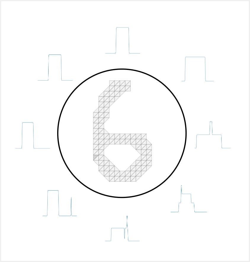
Figure 1: We construct a simplicial from an image of the MNIST data set (using a Delaunay complex construction on the non-zero pixels). For each choice of direction on $S^{1}$, we obtain a Euler Characteristic Curve. The collection of all these curves constitutes the Euler Characteristic Transform. Existing work typically concatenates all these curves to obtain a static feature vector, whereas our method uses them in a differentiable fashion.

Euler characteristic.

Various geometrical or topological properties for characterising simplicial complexes exist. A simple properties is the Euler characteristic, defined as the alternating sum of the number of simplices in each dimension. For a simplicial complex $K$, we define the Euler Characteristic $\chi$ as

$$\chi(K)=\sum_{n=0}(-1)^{k}|K^{n}|,$$ (1)

where $|K^{n}|$ denotes the cardinality of set of $n$-simplices. The Euler characteristic is invariant under homeomorphisms and can be related to other properties of $K$; for instance, $\chi(K)$ can be equivalently written as the alternating sum of the Betti numbers of $K$.

Filtrations.

The Euler characteristic is limited in the sense that it only characterises a simplicial complex $K$ at a single scale. A multi-scale perspective can be seen to enhance the expressivity of the resulting representations. Specifically, given a simplicial complex $K$ and a function $f\colon\mathbb{R}^{n}\to\mathbb{R}$, we obtain a multi-scale view on $K$ by considering the function $\tilde{f}$ as the restriction of $f$ to the $0$-simplices of $K$, and defining $\tilde{f}(\sigma):=\max_{\tau\subset\sigma}\tilde{f}(\tau)$ for higher-dimensional simplices. With this definition, $\tilde{f}^{-1}((-\infty,r])$ is either empty or a non-empty simplicial subcomplex of $K$; moreover, for $r_{1}\leq r_{2}$, we have $\tilde{f}^{-1}((-\infty,r_{1}])\subseteq f^{-1}((-\infty,r_{2}])$. A function $\tilde{f}$ with such properties is known as a filter function, and it induces a filtration of $K$ into a sequence of nested subcomplexes, i.e.

$$\emptyset=K_{0}\subseteq K_{1}\dots\subseteq K_{m-1}\subseteq K_{m}=K.$$ (2)

Since the filter function was extended to $K$ by calculating the maximum, this is also known as the sublevel set filtration of $K$ via $f$. Filter functions can either be learned [22, 23], or they can be defined based on existing geometrical-topological properties of the input data. Calculating invariants alongside this filtration results in substantial improvements of the predictive power of methods. For instance, calculating the homology groups of each $K_{i}$ leads to persistent homology, a shape descriptor for point clouds. However, persistent homology does not exhibit favourable scalability properties, making it hard to gainfully use in practice.

4 Methods

With the Euler characteristic being insufficiently expressive and persistent homology being infeasible to calculate for large data sets, the Euler Characteristic Transform (ECT), created by Turner et al. [36], aims to strike a balance between the two. Given a simplicial complex $K$ and a filter function $f$, the central idea of the ECT is to compute the Euler characteristic alongside a filtration, thus obtaining a curve that serves to characterise a shape. If the vertices of $K$ have coordinates in $\mathbb{R}^{n}$, the ECT is typically calculated based on a parametric filter function of the form

$$\begin{aligned} f\colon S^{n-1}\times\mathbb{R}^{n}&\to\mathbb{R}\\ \xi,x&\mapsto\langle x,\xi\rangle\end{aligned}\quad,$$ (3)

where $\xi$ is a direction (living on a sphere of appropriate dimensionality), and $\langle\cdot,\cdot\rangle$ denotes the standard inner product. For a fixed $\xi$, we write $f_{\xi}:=f(\xi,\cdot)$. Given $h\in\mathbb{R}$, also known as the height, we obtain a filtration of $K$ by computing the preimage $f^{-1}_{\xi}((-\infty,h])$. The ECT is then defined as

$$\begin{aligned} \mathrm{ECT}\colon S^{n-1}\times\mathbb{R}&\to\mathbb{Z},\\ \xi,h&\mapsto\chi\left(f^{-1}_{\xi}\big{(}(-\infty,h]\big{)}\right)\end{aligned}\quad.$$ (4)

If $\xi$ is fixed, we also refer to the resulting curve—which is only defined by a single direction—as the Euler Characteristic Curve (ECC). The ECT is thus the collection of ECCs calculated from different directions. Somewhat surprisingly, it turns out that, given a sufficiently larger number of directions $\xi$ [8], the ECT is injective, i.e. it preserves equality [36, 13].

While the injectivity makes the ECT an advantageous shape descriptor, it is currently only used as a static feature descriptor in machine learning applications, relying on a set of pre-defined directions $\xi$, such as directions chosen on a grid. We adopt a novel perspective here, showing how to turn the ECT into a differentiable shape descriptor that affords the integration into deep neural networks, either as a layer or as a loss term. Our key idea that permits the ECT to be used in a differentiable setting is the observation that it can be written as

$$\begin{aligned} \mathrm{ECT}\colon S^{n-1}\times\mathbb{R}&\to\mathbb{Z}\\ \xi,h&\mapsto\sum_{k}^{\dim K}(-1)^{k}\sum_{\sigma_{k}}\mathbbold{1}_{[f_{\xi}(x_{\sigma_{k}}),\infty)}(h)\end{aligned}\quad,$$ (5)

where $\sigma_{k}$ is a $k$-dimensional and $x_{\sigma_{k}}$ is its corresponding feature vector. Eq. 5 rewrites the ECT as an alternating sum of indicator functions. To see that this is an equivalent definition, it suffices to note that for the $0$-dimensional simplices we indeed get a sum of indicator functions, as the ECT counts how many points are below or above a given hyperplane. This value is also unique, and once a point is included, it will remain included. For the higher-dimensional simplices a similar argument holds. The value of the filter function of a higher-dimensional simplex is fully determined its vertices, and once such a simplex is included by the increasing filter function, it will remain included. This justifies writing the ECT as a sum of indicator functions.

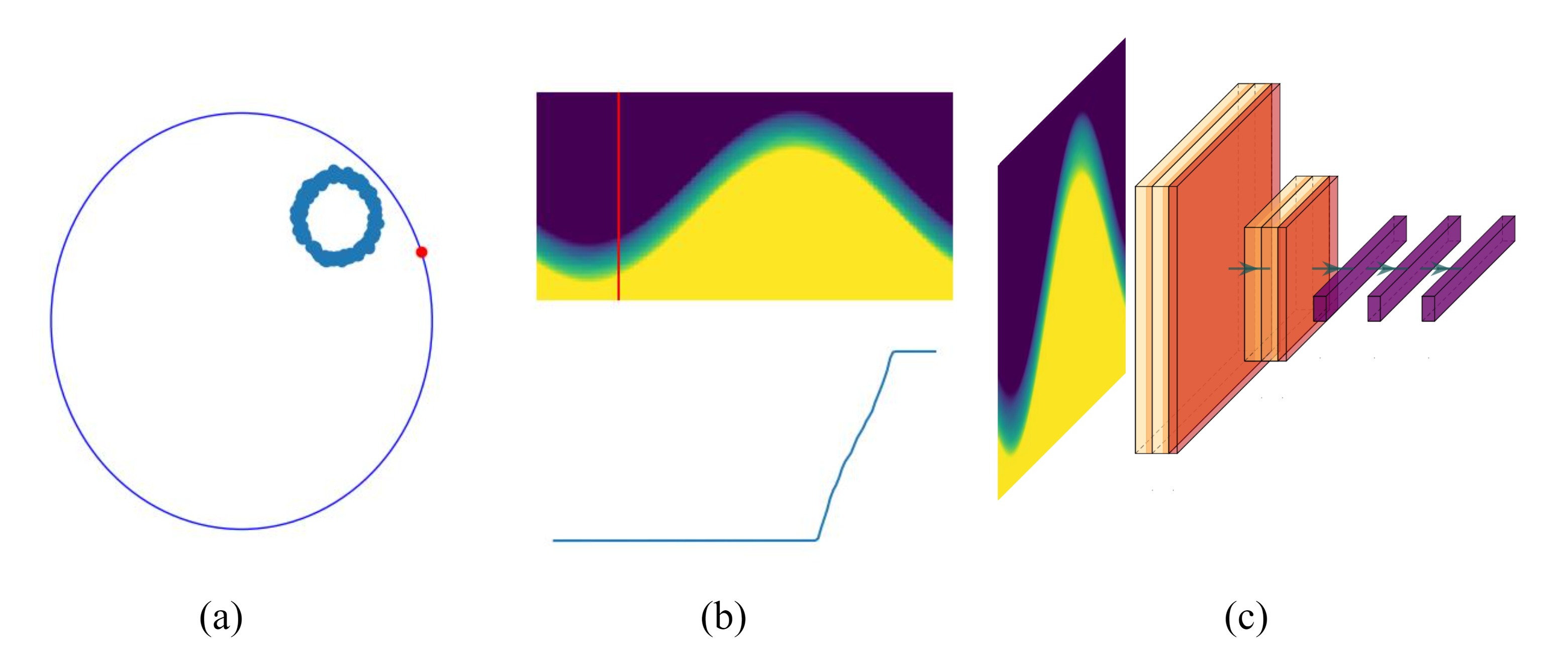
Figure 2: This figure provides an overview for the ECT in a machine learning setting. (a) We are given a noisy point cloud sampled from a circle (blue dots), and a direction on the unit circle (red dot), and compute the ECT in the direction of the red dot to obtain the ECC, the lower figure in (b). Each of curves is stacked and we obtain the curve and the red line in the top of (b) corresponds to the curve below viewed from the top. (c) The resulting 2D image then serves as the input for a CNN that is used to classify the pointcloud.

Differentiability.

A large obstacle towards the development of topological machine learning algorithms involves the integration into deep neural networks, with most existing works treating topological information as mere static features. We want our formulation of the ECT to be differentiable with respect to both the directions $\xi$ as well as the coordinates themselves. However, the indicator function used in LABEL:eq:ECT_indicatorfunctions constitutes an obstacle to differentiability. To overcome this, we replace the indicator function with a sigmoid function, thus obtaining a smooth approximation to the ECT. Notably, this approximation affords gradient calculations. Using a hyperparameter $\lambda$, we can control the tightness of the approximation, leading to

$$\begin{aligned} \mathrm{ECT}\colon S^{n-1}\times\mathbb{R}&\to\mathbb{Z}\\ \xi,h&\mapsto\sum_{k}^{\dim K}(-1)^{k}\sum_{\sigma_{k}}S\left(\lambda\left(h-f_{\xi}(x_{\sigma_{k}})\right)\right)\end{aligned}\quad,$$ (6)

where $S(\cdot)$ denotes the sigmoid function. Each of the summands is differentiable with respect to $\xi$, $x_{\sigma_{k}}$, and $h$, thus resulting in a highly-flexible framework for the ECT. We refer to this variant of the ECT as DECT, i.e. the Differentiable Euler Characteristic Transform.

Our novel formulation can be used in different contexts, which we will subsequently analyse in the experimental section. First, Eq. 6 affords a formulation as a shape descriptor layer, thus enabling representation learning on different domains and making a model ‘topology-aware.’ Second, since Eq. 6 is differentiable with respect to the input coordinates, we can use it to create loss terms and, more generally, optimise point clouds to satisfy certain topological constraints. In contrast to existing works that describe topology-based losses [12, 35, 37, 28], our formulation is highly scalable without requiring subsampling strategies or any form of discretisation in terms of $\xi$ [30].

Integration into deep neural networks.

Next to being differentiable, our novel perspective also lends itself to a better integration into deep neural networks. Traditionally, methods that employ ECTs for classification concatenate the ECCs for different directions into a single vector, which is subsequently used as the input for standard classification algorithms, after having been subjected to dimensionality reduction [1, 24]. However, we find that discarding the directionality information like this results in a loss of crucial information. Moreover, the concatenation of the ECCs requires the dimensionality reduction techniques to be block permutation invariant, as reordering the ECCs should not change the output of the classification. This aspect is ignored in practice, thus losing the interpretability of the resulting representation. By contrast, we aim to make the integration of our variant of the ECT invariant with respect to reordering individual curves. Instead of using a static dimensionality reduction method, we use an MLP to obtain a learnable embedding of individual Euler Characteristic Curves into a high-dimensional space. This embedding is permutation-equivariant by definition. To obtain a permutation-invariant representation, we use a pooling layer, similar to the deep sets architecture [41]. Finally, we use a simple classification network based on another MLP. We note that most topological machine learning architectures require a simplicial complex with additional connectivity information to work. This usually requires additional hyperparameters or, in the case of persistent homology, a sequence of simplicial complexes encoding the data at multiple scales. Other deep learning methods, such as deep sets, require a restriction on the number of points in each sample in the dataset. By contrast, our method can directly work with point clouds, exhibiting no restrictions in terms of the number of points in each object nor any restrictions concerning the type of sample connectivity information. Hence, DECT can handle data consisting of a mixture of point clouds, graphs, or meshes simultaneously.

Computational efficiency and implementation.

While there are already efficient algorithms for the computation of the ECT for certain data modalities, like image and voxel data [39], our method constitutes the first description of a differentiable variant of the ECT in general machine learning settings. Our method is applicable to point clouds, graphs, and meshes. To show that our formulation is computationally efficient, we provide a brief overview on how to implement Eq. 6 in practice:

1. We first calculate the inner product of all coordinates with each of the directions, i.e. with each of the coordinates from $S^{n-1}$.

2. We extend these inner products to a valid filter function by calculating a sublevel set filtration.

3. We translate all indicator functions by the respective filtration value and sample them on a regular grid in the range of the sigmoid function, i.e. in $[-1,1]$. This is equivalent to evaluating $\mathbbold{1}_{[f_{\xi}(\sigma_{k}),1]}$ on the interval $[-1,1]$.

4. Finally, we add all the indicator functions, weighted by $\pm 1$ depending on the dimension, to obtain the ECT.

All these computations can be vectorized and executed in parallel, making our reformulation highly scalable on a GPU.

5 Experiments

Having described a novel, differentiable variant of the Euler Characteristic Transform (ECT), we conduct a comprehensive suite of experiments to explore and assess its properties. First and foremost, building on the intuition of the ECT being a universal shape descriptor, we are interested in understanding how well ECT-based models perform across different types of data sets, such as point clouds, graphs, and meshes. Moreover, while recent work has proven theoretical bounds on the number of directions required to unique classify a shape (i.e. the number of directions required to guarantee injectivity) via the ECT [8], we strive to provide practical insights into how well classification accuracy depends on the number of directions used to calculate the ECT. Finally, we also show how to use the ECT to transform to point clouds, taking on the role of additional optimisation objectives that permit us to adjust point clouds based on a target ECT.

Preprocessing and experimental setup.

We preprocess all data sets so that their vertex coordinates have at most unit norm. We also centre vertex coordinates at the origin. This scale normalisation simplifies the calculating of ECTs and enables us to use simpler implementations. Moreover, given the different cardinalities and modalities of the data, we slightly adjust our training procedures accordingly. We split data sets following an $80\%/20\%$ train/test split, reserving another $20\%$ of the training data for validation. For the graph classification, we set the maximum number of epochs to $100$. We use the ADAM optimiser with a starting learning rate of $0.001$. As a loss term, we either use categorical cross entropy for classification or the mean squared error (MSE) for optimising point clouds and directions.

Architectures.

We showcase the flexibility of DECT by integrating it into different architectures. Our architectures are kept purposefully simple and do not make use of concepts like attention, batch normalisation, or weight decay. For the synthetic data sets, we add DECT as the first layer of an MLP with $3$ hidden layers. For graph classification tasks, we also use DECT as the first layer, followed by two convolutional layers, and an MLP with $3$ hidden layers for classification. By default, we use $16$ different directions for the calculation of the ECT and discretise each curve into $16$ steps. This results in a $16\times 16$ ‘image’ for each input data set. When using convolutional layers, our first convolutional layer has $8$ channels, followed by a layer with $16$ channels, which is subsequently followed by a pooling layer. Our classification network is an MLP with $25$ hidden units per layer and $3$ layers in total. Since we represent each graph as a $16\times 16$ image the number of parameters is always constant in our model, ignoring the variation in the dimension of the nodes across the different datasets. We find that this makes the model highly scalable.

5.1 Classifying Synthetic Manifolds Across Different Modalities

Table 1: DECT can classify three classes of manifolds across three different modalities.

ECT + MLP
Point cloud	$1.0\pm 0.0$
Graph	$1.0\pm 0.0$
Mesh	$1.0\pm 0.0$

As a motivating example, we first showcase the capabilities of DECT to classify synthetically-generated $2$-manifolds. To this end, we generate $2$-spheres, tori, and Möbius strips. In total, the data set consists of $300$ manifolds, distributed equally along the three difference classes. We then represent the objects in the form of point clouds (only vertices), graphs (vertices and edges), and meshes (coordinates, edges, and faces). To improve the complexity of this classification task, we perturb vertex coordinates using a per-coordinate perturbation sampled uniformly from $[0,0.3)$ and a random rotation; this level of perturbation is sufficiently small to prevent major distortions between the two classes. Table 1 depicts the results and we observe that DECT exhibits perfect classification over all three modalities.

5.2 Optimising Euler Characteristic Transforms

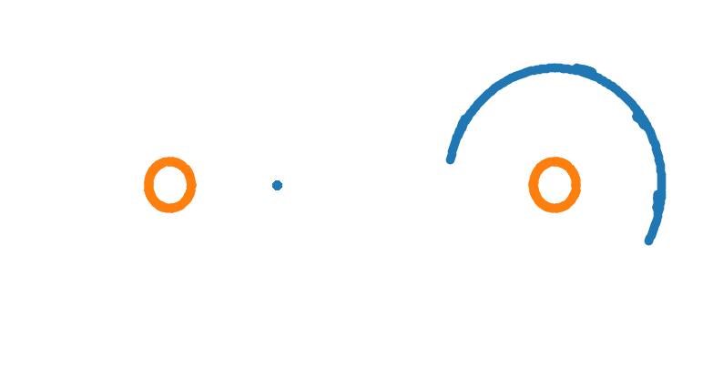
(a) Learning directions

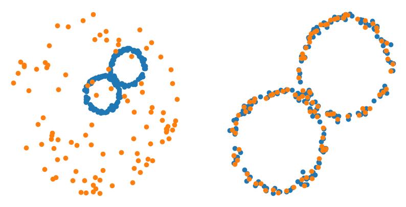
(b) Learning coordinates

Figure 3: 3(a): We sample a noisy point cloud from a circle (orange). Blue dots show the directions, i.e. angles, used for the ECT (left: initial, right: after training). Our method DECT spreads directions properly over the unit circle, resulting in a perfect matching of the ground truth. 3(b): DECT also permits us to optimise existing point clouds to match a target ECT in an end-to-end differentiable fashion. Using two point clouds (blue: target; orange: input data), we train DECT with an MSE loss between the learned ECT and the target ECT. Starting from a randomly-initialised point cloud (left), point coordinates are optimised to match the desired shape (right). Notably, this optimisation only involves the ECT, demonstrating its capabilities as a universal shape descriptor.

Following existing topology-based optimisation methods [12, 28, 5], we also employ DECT in this context. In contrast to existing methods, representations learned by DECT lend itself to better interpretability since one can analyse what directions are using during the classification. The collection of all learned directions can provide valuable insights into the complexity of the data, highlighting symmetries.

Learning and visualising directions.

We fix a noisy point cloud sampled from a circle, computing the full ECT with respect to a set of directions sampled uniformly from $S^{1}$. This corresponds to the ‘ground truth’ ECT. We then initialise our method DECT with a set of directions set to a random point on the unit circle. Using an MSE loss between the ground truth ECT and the ECT used in our model, we may learn appropriate directions. Fig. 3(a) shows the results of the training process. We observe two phenomena: first, due to the symmetry of the ECT, it suffices to only cover half the unit circle in terms of directions; indeed, each vertical slice of the ECT yields an ECC, which can also be obtained by rotation. The same phenomenon occurs, mutatis mutandis, when directions are initialised on the other side of the circle: the axis of symmetry runs exactly through the direction closest and furthest from the point cloud, corresponding to the ‘maximum’ and ‘minimum’ observed in the sinusoidal wave pattern that is apparent in the ground truth ECT. One may observe that the learned directions are not precisely situated on the unit circle; they are only situated close to it. This is due to our model not using a spherical constraint, i.e. learned directions are just considered to be points in $\mathbb{R}^{2}$ as opposed to being angles. However, the optimisation process still forces the directions to converge to the unit circle, underpinning the fact that our novel layer DECT can in fact learn the ECT of an object even if given more degrees of freedom than strictly required.

Optimising point clouds.

To complement the previous experiment on ECT-based optimisation, we also show how to use DECT to optimise point cloud coordinates according to match a desired geometrical-topological descriptor. This type of optimisation can also be seen as an additional regularisation based on topological constraints. In contrast to existing works [37, 28, 35], our method is computationally highly efficient and does not require any additional constructions of simplicial complexes. To showcase the capabilities of DECT as an optimisation objective, we normalise all ECTs, thus ensuring that they operate on the same order of magnitude for an MSE loss. Being differentiable, DECT permits us to adjust the coordinate positions of the source point cloud as a function as of the MSE loss, computed between the ECT of the model and the ECT of the target point cloud. As Fig. 3(b) demonstrates, our method is capable to adjust coordinates appropriately. Notably, this also permits us to train with different sample sizes, thus creating sparse approximations to target point clouds. We leave the approximation of structured objects, such as graphs or simplicial complexes, for future work; the higher complexity of such domains necessitates constructions of auxiliary complexes, which need to be separately studied in terms of differentiability.

5.3 Classifying Geometric Graphs

Table 2: A comparison of our method with other methods on the MNIST-Superpixel data set. We report overall accuracy and runtime per epoch, highlighting the fact that even on commodity hardware, our method is an order of magnitude faster than the fasted GNN methods. This yields a favourable trade-off between performance, scalability, and accuracy. Finally, we find that accuracy can be improved by considering a complex constructed from the input images; in this case, our ECT+MLP method is on a par with more complex graph neural networks, but this comes at the cost of increased runtime (due to the fact that faces have to be added to the data). Accuracy values and runtimes of all all comparison partners are taken from Dwivedi et al. [9].

Method	Accuracy	Epoch runtime ($\mathrm{s}$)
GAT [38]	$95.54$ p m 0.21	$42.26$
GCN [25]	$90.71$ p m 0.22	$83.41$
GIN [40]	$96.49$ p m 0.14	$39.22$
GraphSage [18]	$97.31$ p m 0.10	$113.12$
MLP	$95.34$ p m 0.14	$22.74$
ECT+CNN (ours)	$93.00$ p m 0.80	$4.50$
ECT+MLP (ours)	$97.20$ p m 0.10	$10.80$

Moving from point clouds to graphs, we first study the performance of our method on the MNIST-Superpixel data set [9]. This data set, being constructed from image data, has a strong underlying geometric component, which we hypothesise our model should be capable of leveraging. Next to the graph version, we thus also create a meshed variant of the MNIST-Superpixel data set. To this end, we first assign to each pixel a coordinate in $\mathbb{R}^{2}$ by regularly sampling the unit square. As usual, we set the vertices in the simplicial complex to be the non-zero pixel coordinates. We then add edges and faces by computing a Delaunay complex of the data (the radius of said complex spans the non-zero pixels). The resulting complex captures both the geometry and the topology of the images in the data set. Following this, we classify the data using DECT and other methods, using a CNN architecture for the original data set and an MLP architecture for its meshed version. Interestingly, we found that our method only requires about $20$ epochs for training, after which training is stopped automatically, whereas competitor methods use more of the allocated training budget of $100$ epochs. Table 2 depicts the results; we find that DECT overall exhibits favourable performance given its smaller footprint. Moreover, using the meshed variant of the data set, we observe performance on a par with competitor methods; the presence of higher-order elements like faces enables DECT to leverage geometrical properties of the data better. Finally, we want to point towards computational considerations. The last column of the table shows the runtimes per epoch; here, DECT outperforms all other approaches by an order of magnitude or more. To put this into perspective, the runtime for MNIST has been the slowest in all our experiments, with most training runs for other experiments only taking about a minute for a full $100$ epochs. We report the values from Dwivedi et al. [9] noting that the survey uses a single Nvidia 1080Ti (11GB) GPU was used on a compute cluster, whereas our model was trained on a Nvidia GeForce RTX 3070 Ti (8GB) GPU of a commodity laptop. This underlines the utility of DECT as faster, more efficient classification method.

We also use a minimal version of DECT to classify point clouds. In contrast to existing work [36], we do not use (simplicial) complexes, but restrict the ECT to hyperplanes, essentially merely counting the number of points above or below a given plane for each curve. We then classify shapes from ModelNet40, sampling either $100$ or $1000$ points. In the former case, we achieve an accuracy of $74\pm 0.5$ over $5$ runs, while in the latter case our accuracy is $77.1\pm 0.4$. Given the low complexity and high speed of our model, this is surprisingly close to the performance reported by Zaheer et al. [41], i.e. $82.0\pm 2.0$ and $87.0\pm 2.0$, respectively. Moreover, DECT is not restricted to point clouds of a specific size, and we believe that the performance gap could potentially be closed for models with more pronounced topological features and varying cardinalities.

Figure 4: Accuracy on a ‘Letter-low’ as a function of the number of directions.

As a final experiment, we show the performance of our DECT when it comes to analysing graphs that contain node coordinates. We use several graph benchmark data sets [29], with Table 3 depicting the results. We observe high predictive performance; our model outperforms existing graph neural networks while requiring a smaller number of parameters. We also show the benefits of substantially increasing the capacity of our model; going to a higher parameter budget yields direct improvements in terms of predictive performance. Interestingly, we observe the highest gains on the ‘Letter’ data sets, which are subjected to increasingly larger levels of noise. The high performance of our model in this context may point towards better robustness properties; we aim to investigate this in future work. Finally, as Fig. 4 demonstrates, accuracy remains high even when choosing a smaller number of directions for the calculation of the ECT.

Table 3: Results of $5$ runs on small graph benchmark data sets. Parameter numbers are approximate because the number of classes differs. The high consistency and performance of our method on the ‘Letter’ data sets is notable.

	Params.	BZR	COX2	DHFR	Letter-low	Letter-med	Letter-high
GAT	5K	$80.25$ p m 1.95	$79.23$ p m 2.58	$72.76$ p m 3.20	$90.04$ p m 2.23	$63.69$ p m 5.97	$43.73$ p m 4.13
GCN	5K	$80.49$ p m 2.37	$79.44$ p m 1.78	$76.73$ p m 3.83	$81.38$ p m 1.57	$62.00$ p m 2.07	$43.06$ p m 1.67
GIN	9K	$81.73$ p m 4.89	$77.94$ p m 2.41	$64.69$ p m 8.26	$85.0$ p m 0.6	$67.07$ p m 2.47	$50.93$ p m 3.47
ECT+CNN (ours)	4K	$81.79$ p m 3.19	$70.4$ p m 0.9	$67.93$ p m 4.97	$91.51$ p m 2.08	$76.22$ p m 4.76	$63.82$ p m 6.04
ECT+CNN (ours)	65K	$84.30$ p m 6.10	$74.60$ p m 4.50	$72.90$ p m 1.60	$96.80$ p m 1.20	$86.30$ p m 2.00	$85.40$ p m 1.30

6 Conclusion and Discussion

We described DECT, the first differentiable framework for Euler Characteristic Transforms (ECTs) and showed how to integrate it into deep learning models. Our method is applicable to different data modalities—including point clouds, graphs, and meshes—and we showed its utility in a variety of learning tasks, comprising both optimisation and classification. The primary strength of our method is its flexibility; it can handle data sets with mixed modalities, containing objects with varying sizes and shapes—we find that few algorithms exhibit similar aspects. Moreover, our computation lends itself to high scalability and built-in GPU acceleration; as a result, our ECT-based methods train an order of magnitude faster than existing models on the same hardware. We observe that our method exhibits scalability properties that surpass existing topological machine learning algorithms [19, 17]. Thus, being fully differentiable, both with respect to the number of directions used for its calculation as well as with respect to the input coordinates of a data set, we extend ECTs to hitherto-unavailable applications.

Future work.

We believe that this work paves the path towards new future research directions and variants of the ECT. Along these lines, we first aim to extend this framework to encompass variants like the Weighted Euler Characteristic Transform [24] or the Smooth Euler Characteristic Transform [7]. Second, while our experiments already allude to the use of the ECT to solve inverse problems for point clouds, we would like to analyse to what extent our framework can be used to reconstruct graphs, meshes, or higher-order complexes. Given the recent interest in such techniques due to their characteristic geometrical and topological properties [31], we believe that this will constitute a intriguing research direction. Moreover, from the perspective of machine learning, there are numerous improvements possible. For instance, the ECT in its current form is inherently equivariant with respect to rotations; finding better classification algorithms that respect this structure would thus be of great interest, potentially leveraging spherical CNNs for improved classification [6]. Finally, we aim to improve the representational capabilities of the ECT by extending it to address node-level tasks; in this context, topology-based methods have already exhibited favourable predictive performance at the price of limited scalability [23]. We hope that extensions of DECT may serve to alleviate these issues in the future.

Reproducibility Statement

The code and configurations are provided for our experiments for reproducibility purposes. All experiments were run on a single GPU to prohibit further randomness and all parameters were logged. Our code will be released under a BSD-3-Clause Licence and can be accessed under https://github.com/aidos-lab/DECT.

References

- Amézquita et al. [2022] Erik J Amézquita, Michelle Y Quigley, Tim Ophelders, Jacob B Landis, Daniel Koenig, Elizabeth Munch, and Daniel H Chitwood. Measuring hidden phenotype: quantifying the shape of barley seeds using the Euler characteristic transform. in silico Plants, 4(1):diab033, 2022.
- Barannikov [1994] Serguei A. Barannikov. The framed Morse complex and its invariants. Advances in Soviet Mathematics, 21:93--115, 1994.
- Bodnar et al. [2021a] Cristian Bodnar, Fabrizio Frasca, Nina Otter, Yuguang Wang, Pietro Liò, Guido F Montufar, and Michael Bronstein. Weisfeiler and Lehman go cellular: CW networks. In M. Ranzato, A. Beygelzimer, Y. Dauphin, P.S. Liang, and J. Wortman Vaughan (eds.), Advances in Neural Information Processing Systems, volume 34, pp. 2625--2640. Curran Associates, Inc., 2021a.
- Bodnar et al. [2021b] Cristian Bodnar, Fabrizio Frasca, Yu Guang Wang, Nina Otter, Guido Montúfar, P. Liò, and M. Bronstein. Weisfeiler and Lehman go topological: Message passing simplicial networks. Proceedings of the 38th International Conference on Machine Learning PMLR, 139:1026--1037, 2021b.
- Carrière et al. [2021] Mathieu Carrière, Frédéric Chazal, Marc Glisse, Yuichi Ike, Hariprasad Kannan, and Yuhei Umeda. Optimizing persistent homology based functions. In Marina Meila and Tong Zhang (eds.), Proceedings of the 38th International Conference on Machine Learning (ICML), number 139 in Proceedings of Machine Learning Research, pp. 1294--1303. PMLR, 2021.
- Cohen et al. [2018] Taco S. Cohen, Mario Geiger, Jonas Köhler, and Max Welling. Spherical CNNs. In International Conference on Learning Representations, 2018. URL https://openreview.net/forum?id=Hkbd5xZRb.
- Crawford et al. [2020] Lorin Crawford, Anthea Monod, Andrew X. Chen, Sayan Mukherjee, and Raúl Rabadán. Predicting clinical outcomes in glioblastoma: An application of topological and functional data analysis. Journal of the American Statistical Association, 115(531):1139--1150, 2020.
- Curry et al. [2022] Justin Curry, Sayan Mukherjee, and Katharine Turner. How many directions determine a shape and other sufficiency results for two topological transforms. Transactions of the American Mathematical Society, Series B, 9(32):1006--1043, 2022.
- Dwivedi et al. [2023] Vijay Prakash Dwivedi, Chaitanya K. Joshi, Anh Tuan Luu, Thomas Laurent, Yoshua Bengio, and Xavier Bresson. Benchmarking Graph Neural Networks. Journal of Machine Learning Research, 24(43):1--48, 2023.
- Ebli et al. [2020] Stefania Ebli, Michaël Defferrard, and Gard Spreemann. Simplicial neural networks. In NeurIPS Workshop on Topological Data Analysis & Beyond, 2020. URL https://openreview.net/forum?id=nPCt39DVIfk.
- Edelsbrunner & Harer [2010] Herbert Edelsbrunner and John Harer. Computational topology: An introduction. American Mathematical Society, Providence, RI, USA, 2010.
- Gabrielsson et al. [2020] Rickard Brüel Gabrielsson, Bradley J. Nelson, Anjan Dwaraknath, and Primoz Skraba. A topology layer for machine learning. In Silvia Chiappa and Roberto Calandra (eds.), Proceedings of the 23rd International Conference on Artificial Intelligence and Statistics (AISTATS), number 108 in Proceedings of Machine Learning Research, pp. 1553--1563. PMLR, 2020.
- Ghrist et al. [2018] Robert Ghrist, Rachel Levanger, and Huy Mai. Persistent homology and euler integral transforms. Journal of Applied and Computational Topology, 2(1):55--60, 2018.
- Guo et al. [2021] Yulan Guo, Hanyun Wang, Qingyong Hu, Hao Liu, Li Liu, and Mohammed Bennamoun. Deep learning for 3d point clouds: A survey. IEEE Transactions on Pattern Analysis and Machine Intelligence, 43(12):4338--4364, 2021.
- Hacker [2020] Celia Hacker. $k$-simplex2vec: a simplicial extension of node2vec. In NeurIPS Workshop on Topological Data Analysis & Beyond, 2020. URL https://openreview.net/forum?id=Aw9DUXPjq55.
- Hajij et al. [2020] Mustafa Hajij, Kyle Istvan, and Ghada Zamzmi. Cell complex neural networks. In NeurIPS Workshop on Topological Data Analysis & Beyond, 2020. URL https://openreview.net/forum?id=6Tq18ySFpGU.
- Hajij et al. [2023] Mustafa Hajij, Ghada Zamzmi, Theodore Papamarkou, Nina Miolane, Aldo Guzmán-Sáenz, Karthikeyan Natesan Ramamurthy, Tolga Birdal, Tamal K. Dey, Soham Mukherjee, Shreyas N. Samaga, Neal Livesay, Robin Walters, Paul Rosen, and Michael T. Schaub. Topological Deep Learning: Goiny beyond graph data. arXiv preprint, pp. arXiv:2206.00606, 2023.
- Hamilton et al. [2017] Will Hamilton, Zhitao Ying, and Jure Leskovec. Inductive representation learning on large graphs. In I. Guyon, U. Von Luxburg, S. Bengio, H. Wallach, R. Fergus, S. Vishwanathan, and R. Garnett (eds.), Advances in Neural Information Processing Systems, volume 30. Curran Associates, Inc., 2017.
- Hensel et al. [2021] Felix Hensel, Michael Moor, and Bastian Rieck. A survey of topological machine learning methods. Frontiers in Artificial Intelligence, 4:681108, 2021.
- Hofer et al. [2017] Christoph Hofer, Roland Kwitt, Marc Niethammer, and Andreas Uhl. Deep learning with topological signatures. In I. Guyon, U. V. Luxburg, S. Bengio, H. Wallach, R. Fergus, S. Vishwanathan, and R. Garnett (eds.), Advances in Neural Information Processing Systems 30 (NeurIPS), pp. 1634--1644. Curran Associates, Inc., Red Hook, NY, USA, 2017.
- Hofer et al. [2019] Christoph Hofer, Roland Kwitt, Marc Niethammer, and Mandar Dixit. Connectivity-optimized representation learning via persistent homology. In Kamalika Chaudhuri and Ruslan Salakhutdinov (eds.), Proceedings of the 36th International Conference on Machine Learning, number 97 in Proceedings of Machine Learning Research, pp. 2751--2760. PMLR, 2019.
- Hofer et al. [2020] Christoph D. Hofer, Florian Graf, Bastian Rieck, Marc Niethammer, and Roland Kwitt. Graph filtration learning. In Hal Daumé III and Aarti Singh (eds.), Proceedings of the 37th International Conference on Machine Learning, number 119 in Proceedings of Machine Learning Research, pp. 4314--4323. PMLR, 2020.
- Horn et al. [2022] Max Horn, Edward De Brouwer, Michael Moor, Yves Moreau, Bastian Rieck, and Karsten Borgwardt. Topological graph neural networks. In International Conference on Learning Representations, 2022. URL https://openreview.net/forum?id=oxxUMeFwEHd.
- Jiang et al. [2020] Q. Jiang, S. Kurtek, and T. Needham. The weighted Euler curve transform for shape and image analysis. In Proceedings of the IEEE/CVF Conference on Computer Vision and Pattern Recognition Workshops (CVPRW), pp. 3685--3694, 2020.
- Kipf & Welling [2017] Thomas N. Kipf and Max Welling. Semi-Supervised Classification with Graph Convolutional Networks. In International Conference on Learning Representations, 2017. URL https://openreview.net/forum?id=SJU4ayYgl.
- Kirveslahti & Mukherjee [2023] Henry Kirveslahti and Sayan Mukherjee. Representing fields without correspondences: the lifted euler characteristic transform. Journal of Applied and Computational Topology, 2023.
- Marsh et al. [2022] Lewis Marsh, Felix Y Zhou, Xiao Quin, Xin Lu, Helen M Byrne, and Heather A Harrington. Detecting temporal shape changes with the euler characteristic transform. arXiv preprint arXiv:2212.10883, 2022.
- Moor et al. [2020] Michael Moor, Max Horn, Bastian Rieck, and Karsten Borgwardt. Topological autoencoders. In Hal Daumé III and Aarti Singh (eds.), Proceedings of the 37th International Conference on Machine Learning, number 119 in Proceedings of Machine Learning Research, pp. 7045--7054. PMLR, 2020.
- Morris et al. [2020] Christopher Morris, Nils M Kriege, Franka Bause, Kristian Kersting, Petra Mutzel, and Marion Neumann. TUDataset: A collection of benchmark datasets for learning with graphs. arXiv preprint arXiv:2007.08663, 2020.
- Nadimpalli et al. [2023] Kalyan Varma Nadimpalli, Amit Chattopadhyay, and Bastian Rieck. Euler characteristic transform based topological loss for reconstructing 3d images from single 2d slices. In Proceedings of the IEEE/CVF Conference on Computer Vision and Pattern Recognition, pp. 571--579, 2023.
- Oudot & Solomon [2020] Steve Oudot and Elchanan Solomon. Inverse problems in topological persistence. In Nils A. Baas, Gunnar E. Carlsson, Gereon Quick, Markus Szymik, and Marius Thaule (eds.), Topological Data Analysis, pp. 405--433, Cham, Switzerland, 2020. Springer.
- Papillon et al. [2023] Mathilde Papillon, Sophia Sanborn, Mustafa Hajij, and Nina Miolane. Architectures of topological deep learning: A survey on topological neural networks. arXiv preprint arXiv:2304.10031, 2023.
- Reininghaus et al. [2015] Jan Reininghaus, Stefan Huber, Ulrich Bauer, and Roland Kwitt. A stable multi-scale kernel for topological machine learning. In IEEE Conference on Computer Vision and Pattern Recognition (CVPR), pp. 4741--4748, Red Hook, NY, USA, June 2015. Curran Associates, Inc.
- Skraba & Turner [2020] Primoz Skraba and Katharine Turner. Wasserstein stability for persistence diagrams. arXiv preprint arXiv:2006.16824, 2020.
- Trofimov et al. [2023] Ilya Trofimov, Daniil Cherniavskii, Eduard Tulchinskii, Nikita Balabin, Evgeny Burnaev, and Serguei Barannikov. Learning topology-preserving data representations. In International Conference on Learning Representations, 2023. URL https://openreview.net/forum?id=lIu-ixf-Tzf.
- Turner et al. [2014] Katharine Turner, Sayan Mukherjee, and Doug M. Boyer. Persistent homology transform for modeling shapes and surfaces. Information and Inference: A Journal of the IMA, 3(4):310--344, 12 2014.
- Vandaele et al. [2022] Robin Vandaele, Bo Kang, Jefrey Lijffijt, Tijl De Bie, and Yvan Saeys. Topologically regularized data embeddings. In International Conference on Learning Representations, 2022. URL https://openreview.net/forum?id=P1QUVhOtEFP.
- Veličković et al. [2018] Petar Veličković, Guillem Cucurull, Arantxa Casanova, Adriana Romero, Pietro Liò, and Yoshua Bengio. Graph attention networks. In International Conference on Learning Representations, 2018. URL https://openreview.net/forum?id=rJXMpikCZ.
- Wang et al. [2022] Fan Wang, Hubert Wagner, and Chao Chen. GPU computation of the euler characteristic curve for imaging data. In Xavier Goaoc and Michael Kerber (eds.), 38th International Symposium on Computational Geometry (SoCG), volume 224 of LIPIcs, pp. 64:1--64:16, 2022.
- Xu et al. [2019] Keyulu Xu, Weihua Hu, Jure Leskovec, and Stefanie Jegelka. How Powerful are Graph Neural Networks? In International Conference on Learning Representations, 2019. URL https://openreview.net/forum?id=ryGs6iA5Km.
- Zaheer et al. [2017] Manzil Zaheer, Satwik Kottur, Siamak Ravanbakhsh, Barnabas Poczos, Russ R Salakhutdinov, and Alexander J Smola. Deep sets. In I. Guyon, U. Von Luxburg, S. Bengio, H. Wallach, R. Fergus, S. Vishwanathan, and R. Garnett (eds.), Advances in Neural Information Processing Systems, volume 30. Curran Associates, Inc., 2017.
- Zhou et al. [2020] Jie Zhou, Ganqu Cui, Shengding Hu, Zhengyan Zhang, Cheng Yang, Zhiyuan Liu, Lifeng Wang, Changcheng Li, and Maosong Sun. Graph neural networks: A review of methods and applications. AI Open, 1:57--81, 2020.