Surgery Constructions for 3d Theories, Part I: Matter Circles and Links

Abstract

We try to give a geometric construction of 3d $\mathcal{N}=2$ gauge theories using three-manifolds and Dehn surgeries. It is known that wrapping M5-branes on plumbing three-manifolds leads to 3d theories with mixed Chern-Simons levels. We find that this construction can be extended by adding Lagrangian defects on the tangent bundles of three-manifolds. After wrapping M5-branes on these defects and through M-theory/IIB string duality, one can get D5-branes that introduce chiral multiplets. This is analogous to Ooguri-Vafa construction of Wilson loop operators along knots on the three-sphere. In this note, we only consider unknotted matter circles, which are intersections between defect M5-branes and plumbing manifolds. After introducing matters, mirror dualities of 3d theories match with Kirby moves of plumbing manifolds. We also find the dictionary between various structures of three-manifolds and physical aspects of 3d gauge theories.

1 Introduction

There are already many distinguished works on 3d $\mathcal{N}=2$ gauge theories e.g. Intriligator:1996ex ; Aharony:1997aa ; Hanany:1996ie ; Kapustin:1999ha ; Dorey:1999rb ; Giveon_2009 ; Benini:2011aa ; Intriligator:2013lca ; Alday:2017yxk . However the geometric engineering is not very well established yet. Brane webs for some examples are known in e.g.Boer:1997ts ; Benvenuti:2016wet ; Cheng:2021vtq , while at this stage brane webs cannot encode mixed Chern-Simons levels and generic superpotentials. We think theree-manifolds are promising because of the fruitful geometric structures and transformations, such as Kirby moves kirbymove . We try to propose a new construction based on Dehn surgeries in complement with DGG/GPV construction given by 3d-3d correspondence Dimofte:2011ju ; Gukov:2016ad ; Cecotti:2011iy ; Terashima:2011qi . Basically, surgery construction is also the compactification of 6d $(2,0)$ theories on three-manifolds. Putting M5-branes on some three-manifolds such as Lens spaces could lead to 3d $\mathcal{N}=2$ gauge theories. M5-branes can also wrap generic three-manifolds, such as plumbing manifolds to generate colorful 3d theories. In recent years, there are attentions on computing the WRT invariants of plumbing manifolds Gukov:2016ad ; Gukov:2017aa ; Cheng:2018aa . On the physical side, linking numbers of these plumbing manifolds are interpreted as the mixed Chern-Simons levels of 3d theories Gadde:2013aa . In our previous work Cheng:2023ocj , we extend this story by introducing chiral multiplets and gauging basic mirror dualities. To describe these introduced matter fields, we found plumbing graphs should be extended by adding gray boxes to denote chiral multiplets, as shown in Figure 2. We also found that in the presence of these new objects, some physical dualities match very well with the first type Kirby moves of three-manifolds. This implies that the introduced gray boxes are necessary and should have geometric interpretations. However, in Cheng:2023ocj , the existence of gray boxes (matter nodes) on three-manifolds is a conjecture. In this note, we fill this gap by exploring the geometric engineering of matters, and find these chiral multiplets should correspond to some codimensional-two defects given by wrapping M5-branes on the tangent bundle of three-manifolds.

To solve this problem, many steps need to be done for finding the dictionary between three-manifolds and 3d gauge theories. We firstly notice that the charges of chiral multiplets under gauge groups should be interpreted as winding numbers. This can be known by analyzing Kirby moves and in particular the handle-slides of circles kirbymove . This step is helpful to interpret geometric transformations as physical dualities, such as $ST$-moves (gauged mirror duality) Cheng:2023ocj . To get some geometric objects that have winding numbers, we should at least consider loops as candidates. We use the M-theory/IIB string dualities to figure out that some Lagrangian defects satisfy this property, which are analogous to Ooguri-Vafa’s constructions Ooguri:1999bv of Wilson loops by introducing Lagrangian M5-branes to intersect the three-sphere along knots $L_{K}\cap S^{3}=K$. In our context, the defects intersect three-manifolds along some circles $L_{\color[rgb]{1,0,0}\circ}\cap M_{3}={\color[rgb]{1,0,0}{\bigcirc}}$, which fully characterize chiral multiplets and hence we call them matter circles. These defects can be checked and confirmed by dualing M5-brane webs to 3d brane webs in IIB string theory. The defect M5-brane is then dual to the D5-brane. This looks nice, as strings between D3-brane and D5-brane provide chiral multiplets. Moreover, there are various ways to put these matter circles on $M_{3}$, which engineer chiral multiplets of charges $q_{i}$ under the $i$-th gauge group $U(1)_{i}$. To see how these circles tangle with three-manifolds, Dehn surgeries have to be considered as all closed orientable three-manifolds can be obtained by Dehn surgeries along links of circles. These circles give gauge groups $U(1)\times\cdots\times U(1)$, and hence we call them gauge circles. Matter circles should link to gauge circles, otherwise matters are decoupled. We notice only $S^{3}$ is special and natural for carrying matter defects, which could even give a geometric derivation of $ST$-moves.

More explicitly, Ooguri-Vafa defects giving flavor symmetries should be combined with the Dehn surgeries of three-manifolds to complete the geometric engineering . We illustrate the surgery construction in Figure 1. The left graph shows the Dehn surgery construction of three-manifolds $M_{3}$, which is defined by drilling out the neighborhood of a knot $K$, and then a solid torus is filled in. The right graph shows that the codimensional-two defect $L$ can be introduced to intersect the solid torus. When this solid torus is glued back to form the closed three-manifold $M_{3}$, flavor symmetry is introduced and the chiral multiplet is geometrically realized.

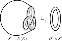
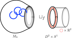
Figure 1: Left graph is the surgery construction of three-manifolds. Right graph shows the surgery construction of the 3d theories with matters.

It is convenient to use plumbing graphs (which are quiver diagrams) to represent 3d theories given by three-manifolds and defects. We illustrate an example in Figure 2. The main ingredients that we introduce are the non-compact defects on the tangent bundle $T^{*}M_{3}$. The three-manifold is given by Dehn surgeries along unknotted links of gauge circles, namely $M_{3}=\left(S^{3}\backslash N({{\color[rgb]{0,0,1}{\bigcirc}}}_{i})\right)\bigcup_{f_{i}}(D_{2}\times S^{1})_{i}$ where we have filled in solid tori to make it compact and hence $\partial M_{3}=\emptyset$.

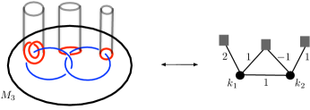
Figure 2: Blue circles ${\color[rgb]{0,0,1}{\bigcirc}}$ are gauge circles for surgeries. Gray cylinders denote Lagrangian defects $L\subset T^{*}M_{3}$. Red circles ${\color[rgb]{1,0,0}{\bigcirc}}$ as intersections of defects with $M_{3}$ are matter circles. This geometry corresponds to a 3d theory with gauge group $U(1)_{k_{1}}\times U(1)_{k_{2}}$ and three chiral multiplets $\Phi_{i}$ of charges $(q_{i}^{1},q_{i}^{2})$. One can represent this theory by its plumbing graph.

We show the dictionary between geometry and gauge theories in Table 1.

three-manifolds plumbing graphs abelian gauge theories matter circle $\color[rgb]{1,0,0}\bigcirc$ $\color[rgb]{.5,.5,.5}\blacksquare$ chiral multiplet F gauge circle $\color[rgb]{0,0,1}\bigcirc$ ${\bullet}_{k_{i}}$ gauge group $U(1)_{k_{i}}$ winding num. between $\color[rgb]{1,0,0}\bigcirc$ and $\color[rgb]{0,0,1}\bigcirc$ charges $q_{i}$ of fund. rep. linking num. between $\color[rgb]{0,0,1}\bigcirc$ and $\color[rgb]{0,0,1}\bigcirc$ effective CS levels $k_{ij}$ $\alpha$-Kirby moves on $\color[rgb]{0,0,1}\bigcirc$ blow up/down of $\bullet_{k}$ integrate in/out $U(1)_{k}$ rational equivalent surgery (89) $ST$-moves (90) gauged mirror triality handle-slides of $\color[rgb]{1,0,0}\bigcirc$ (93) add ${\color[rgb]{.5,.5,.5}\blacksquare}$ add chiral multiplets

Table 1: The dictionary between three-manifolds, plumbing graphs (which can be viewed as quiver diagrams), and gauge theories.

In section 2 we show the winding numbers between matter and gauge circles can be interpreted as charges by considering the handle-slide operation, which is the second type of Kirby moves. In section 3 we use M-theory/IIB string duality and brane webs to show that Lagrangian defect M5-branes along circles are dual to D5-branes, and hence engineer chiral multiplets. In section 4 we discuss the locations of matter circles and gauge circles on plumbing three-manifolds given by Dehn surgeries. We will also give a geometric derivation of $ST$-moves, in which we use a drilling trick and rational equivalent surgeries.

2 Charges as winding numbers

In this section, we briefly review the $ST$-moves, and discuss another type of Kirby moves — handle-slides that have not been addressed in physical literature. We found that handle-slides can be used as an geometric operation to introduced matter nodes to plumbing graphs, and the charges of matters can be interpreted as winding numbers. This implies that matter nodes can be viewed as some kinds of circles, which motivates us to find their geometric realizations. This section contains the background for other sections.

2.1 Mirror triality and $ST$-moves

Before taking about the geometric aspects, let us present what we already know about 3d gauge theories. A well know duality is the basic mirror duality between a free chiral multiplet and a $U(1)$ theory with a charge-1 fundamental chiral multiplet.

$$1\textbf{F}\leavevmode\nobreak\ \leavevmode\nobreak\ \longleftrightarrow\leavevmode\nobreak\ \leavevmode\nobreak\ U(1)_{\pm\frac{1}{2}}+1\textbf{F}$$ (1)

It is convenient to use plumbing graphs to denote this mirror duality:

(2)

where the numbers $\pm 1/2$ are bare Chern-Simons levels. This duality is found in Dimofte:2011ju by decoupling the antifundamental matter $1\textbf{AF}$ in the $\mathcal{N}=2$ representation of the basic $\mathcal{N}=4$ dual pair:

$$1\textbf{F}+1\textbf{AF}\leavevmode\nobreak\ \leavevmode\nobreak\ \longleftrightarrow\leavevmode\nobreak\ \leavevmode\nobreak\ U(1)_{0}+1\textbf{F}+1\textbf{AF}\,.$$ (3)

It is noticed and extensively used in Cheng:2020aa ; Cheng:2023ocj that after gauging the $U(1)$ global symmetry on both side of (1), a new duality is obtained:

(4)

where $q$ is the charge of the matter under the gauge group. The mirror duality (1) corresponds to the operator $ST\in SL(2,\mathbb{Z})$ Witten:2003ya and hence the gauged version (4) is called $ST$-move. We can use plumbing graphs to denote this gauged duality, see Table 1 for details of the notation. Note that in (4), we have assigned the bare Chern-Simons levels. In the following sections, we will only use the effective Chern-Simons levels which receive corrections from all chiral multiplets by the formula Intriligator:1996ex :

$$k^{\text{eff}}=k^{\text{bare}}+\sum_{I=1}^{N_{f}}\frac{q^{2}}{2}\,\text{sign}(q_{I})\text{sign}(m_{I})\,.$$ (5)

2.2 Handle-slides: $\mathbb{\beta}$-Kirby move

For given three-manifolds that can be obtained by Dehn surgeries on links, such as the one in Figure 2. There are Kirby moves on this link to transform it into other links, while the three-manifolds is invariant kirbymove , so Kirby moves are geometrically equivalent operations. Kirby moves contains two types, which are called first and second types, while we call them $\alpha$-type and $\beta$-type in this note for convenience. The $\alpha$-type is discussed in Gadde:2013aa ; Cheng:2023ocj . Basically, $\alpha$-Kirby moves introduce or reduce black nodes of plumbing graphs, which can be interpreted as integrating in/out gauge symmetries, and the $ST$-move reduces to a special case of $\alpha$-Kirby moves if matter nodes are decoupled. However, generic $\alpha$-Kirby moves do not match the duality (4) if matter nodes are present.

The $\beta$-type of Kirby moves is often called handle-slide. In literature kirbymove , $\beta$-type Kirby move is the operation of recombining some components of the links for Dehn surgeries, which can be illustrated in the graph below

$$\begin{split}\includegraphics[width=216.81pt]{figgeo/betakirby.pdf}\end{split}$$ (6)

Let us use $L_{1}$ and $L_{2}$ to denote these two circles. Their framing numbers and linking numbers are as follows

$$L_{1}\cdot L_{1}=r\,,\leavevmode\nobreak\ \leavevmode\nobreak\ L_{1}\cdot L_{2}=L_{2}\cdot L_{1}=k\,,\leavevmode\nobreak\ \leavevmode\nobreak\ L_{2}\cdot L_{2}=s\,.$$ (7)

After $\beta$-type Kirby move, the circle $L_{1}$ is unchanged, while $L_{2}$ combines with $L_{1}$ to form a new circle $\tilde{L}_{2}=L_{2}\pm L_{1}$. Using (7), one can compute linking numbers between new cycles:

$$L_{1}\cdot L_{1}=r\,,\leavevmode\nobreak\ \leavevmode\nobreak\ L_{1}\cdot{\widetilde{L}}_{2}={\widetilde{L}}_{2}\cdot L_{1}=k\pm r\,,\leavevmode\nobreak\ \leavevmode\nobreak\ \tilde{L}_{2}\cdot{\widetilde{L}}_{2}=r+s\pm 2k\,.$$ (8)

These changes are assigned on graphs in (6).

It is hard to physically understand this type of Kirby move, although it can partly be integrated as integrating out gauge nodes. One can check that if integrating out the node $U(1)_{r}$, then the two graphs in (6) reduce to the same one:

(9)

so this $\beta$-Kirby move has overlaps with $\alpha$-Kirby move, but not equivalent to, since $\alpha$-Kirby moves add or reduce gauge nodes, while $\beta$-Kirby move keeps the number of gauge nodes.

One can try to see if other combination of circles works. It is easy to find that $\tilde{L}_{2}=L_{2}+nL_{1}$ with $n\in\mathbb{Z}$ could also lead to the node $U(1)_{s-\frac{k^{2}}{r}}$, if one integrates out $U(1)_{r}$. This gives a generic version of $\beta$-Kirby moves:

(10)

From another perspective, this move can be viewed as iteratively applying the original $\beta$-Kirby move for $n$ times. Note that the reverse process from the right to left is also a $\beta$-Kirby move, as $n$ can be any negative integer.

There is a special case that when $k=0$ and $n=1$, $\alpha$-Kirby move and $\beta$-Kirby move can be directly related $K_{\alpha}\simeq K_{\beta}$:

(11)

since in this case, the $\bullet_{r}$ is disconnected. It could be more better if $r=\pm 1$, as connecting a three-sphere $S^{3}$ to the three-manifold $M_{3}$ is always equivalent to itself, namely $S^{3}\#M_{3}=M_{3}$, and then $K_{\alpha}=K_{\beta}$.

2.3 $\beta$-Kirby introduces matter

In the process of $\beta$-Kirby move, the cycle $L_{1}$ is not affected, while $L_{2}$ changes significantly. However, it is safe to attach a matter to $L_{2}$, as $L_{1}$ can be integrated out. If the matter is on $L_{1}$

(12)

it is hard to know if this is an equivalent operation. We will give an example soon to show this is not an equivalence.

One can use $ST$-moves to understand $\beta$-Kirby moves with matter. Let us first consider the basic $ST$-move:

(13)

where we have assigned effective Chern-Simons levels. Since $ST$-move reduces to $\alpha$-Kirby move after decoupling the matter node, we can denote it as $ST_{\alpha}$. The circle for $ST$-move changes as follows:

$$\{L_{1}\}\leavevmode\nobreak\ \leavevmode\nobreak\ \xrightarrow{ST_{\alpha}}\leavevmode\nobreak\ \leavevmode\nobreak\ \{L_{1}+L\,,L\}\,,$$ (14)

for which $\{L^{2}=\pm 1\,,L_{1}^{2}=k\,,L\cdot L_{1}=0\}$. An interesting property is that after the $ST_{\alpha}$, the matter node ${\color[rgb]{.5,.5,.5}\blacksquare}$ moves from circle $L_{1}$ to circle $L$ in (13). The circles can also recombine in a similar way as the $\beta$-Kirby move in (10), so we propose $ST_{\beta}$-move:

(15)

which is a special $\beta$-Kirby move with $\{r=1,n=1\}$, and a matter node is attached. Here $r$ can also be $-1$, then it corresponds to $(ST)^{2}$-move . The circles under $\beta$-Kirby move change:

$$\{L,L_{1}\}\leavevmode\nobreak\ \leavevmode\nobreak\ \xrightarrow{ST_{\beta}}\leavevmode\nobreak\ \leavevmode\nobreak\ \{L\,,L+L_{1}\}\,,$$ (16)

for which $\{L^{2}=+1\,,L_{1}^{2}=k\,,L\cdot L_{1}=0\}$. During the $ST_{\beta}$-move, the matter node is always on $L$. The $ST_{\beta}$-move is a special case of (12). By comparing (13) and (15), one can see that $ST_{\beta}$-move is not an equivalent operation, since $\bullet_{+1}-{\color[rgb]{.5,.5,.5}\blacksquare}\neq\bullet_{k}-{\color[rgb]{.5,.5,.5}\blacksquare}$, although in the absence of matter nodes, $\beta$-Kirby moves are equivalent operations. When the matter is very massive and decoupled, $ST_{\beta}$-move reduces to a $\beta$-Kirby move. This $ST_{\beta}$-move seems weird, as the decorated node $\bullet_{+1}-{\color[rgb]{.5,.5,.5}\blacksquare}$ on the left graph is disconnected to $\bullet_{k}$, while this decorated note links to it on the right graph of (15). Hence the $ST_{\beta}$ should be viewed an operation of introducing matter nodes to plumbing graphs. Obviously, since $ST_{\beta}$ is not an equivalent operation, and hence is not a duality, while $ST_{\alpha}$-move is a duality as it preserves partition functions.

A naive observation is that one can combine $ST_{\alpha}$ and $ST_{\beta}$, which is an operation of sliding (introducing) a matter node ${\color[rgb]{.5,.5,.5}\blacksquare}$ from $\bullet_{+1}$ to the gauge node $\bullet_{k}$:

(17)

Geometrically, this combined operation changes the position of the matter node from circle $L$ to $L_{1}$. In other words, this combined operation can be viewed as an operation that introduces a matter node to a gauge node $L_{1}$. Note that when the matter node is introduced, the bare CS level $k$ is lifted to the effective CS level. Namely, the bare CS level shifts from $k$ to $k\pm 1/2$.

Moreover, the matter with charge $q$ can also be introduced, and we only need to apply the $ST_{\beta}$-move $q$ times. To get this conclusion, let us consider $(ST_{\beta})^{q}$-moves, which combine circles as follows

$$\widetilde{L}=L\,,\leavevmode\nobreak\ \leavevmode\nobreak\ \widetilde{L}_{1}=L_{1}+qL\,,$$ (18)

whose linking numbers are $\{L\cdot L=+1\,,\leavevmode\nobreak\ \widetilde{L}\cdot\widetilde{L}_{1}=q\,,\leavevmode\nobreak\ \widetilde{L}_{1}\cdot\widetilde{L}_{1}=k+q^{2}\}$. If an external gauge node (circle) $L_{2}$ joins in, then plumbing graphs change as follows:

(19)

Setting $a=0$ and $b=0$ could remove the external node and reduces the above graph to an effective version of the $ST_{\alpha}$-moves in (4) :

(20)

Combining (19) and (20), one can see that $(ST_{\beta})^{q}$ introduces a charge $q$ matter to $\bullet_{k}$:

(21)

This charge is the multiple number of the circle $L\in\widetilde{L}_{1}$, and is also the winding number between $\widetilde{L}$ and $\widetilde{L}_{1}$. One can also couple the matter node to many gauge nodes to form the matter with a charge $q_{i}$ under each $U(1)_{k_{i}}$. For instance, the bifundatmental matter can be introduced by $ST_{\beta}$-moves (handle-slides) below

(22)

where we have assigned effective CS levels. The recombined circles are

$$\widetilde{L}=L\,,\leavevmode\nobreak\ \leavevmode\nobreak\ \widetilde{L}_{1}=L_{1}+q_{1}L\,,\leavevmode\nobreak\ \leavevmode\nobreak\ \widetilde{L}_{2}=L_{2}+q_{2}L\,.$$ (23)

In addition, one can add many matter nodes using handle-slides ($ST_{\beta}$-moves). Recall that introducing or removing $\pm 1$ gauge nodes $\bullet_{\pm 1}$ do not change the three-manifolds. However in the presence of matter nodes on $\bullet_{\pm 1}-{\color[rgb]{.5,.5,.5}\blacksquare}$, this property is somehow broken, since bare CS levels $k_{i}$ are lifted to effective CS levels $k_{i}$. Namely bare CS levels are shifted by the matter node. This looks strange, but can be understood through 3d brane webs; see Cheng:2021vtq .

From the above examples, one can see that both types of Kirby moves have physical interpretations. One can conjecture that the matter node should be some kinds of circles on three-manifolds, because the charge $q_{i}$ is surprisingly interpreted as the winding numbers between the matter and gauge circles $\bullet_{k_{i}}$. Since the matter node ${\color[rgb]{.5,.5,.5}\blacksquare}$ can be viewed as $\bullet_{\pm 1}-{\color[rgb]{.5,.5,.5}\blacksquare}$ through mirror duality (2), matter circles can indirectly use this gauge node $\bullet_{+1}$ to link gauge nodes. In following sections and in particular section 4.4, we will show that matter circles do indeed exist and are given by intersections between Lagrangian defects and three-manifolds, as is illustrated in Figure 2.

Effective and bare $ST$-moves. In this note, we only consider circles with integral framing and linking numbers, and hence they are effective CS levels, while in gauge theory analysis, one can also use bare CS levels and then counts the corrections from matters. At this stage, we do not clearly know how to geometrically describe bare CS levels (bare linking numbers), but we can mention some differences below.

The above examples in this section have shown that the handle-slides ($\beta$-Kirby moves) work and match with effective CS levels of 3d theories. If using bare CS levels, we think it is not easy to see how the corrections from matters emerge. However, both effective version and bare version have benefits and drawbacks. For the bare version of $ST$-moves shown in (4), one can perform $ST_{\alpha}$-moves recursively to form the chain $\bullet_{k\pm q^{2}/2}-\bullet_{\pm 1}-\cdots-\bullet_{\pm 1}-{\color[rgb]{.5,.5,.5}\blacksquare}$, although finally all $\bullet_{\pm 1}$ can be integrated out, and only two types of moves left as shown in (4). However, one cannot consistently do that for the effective version shown in (20). For the effective version, $ST_{\beta}$-moves can be interpreted geometrically as handle-slides, and performing handle-slides many times just means increase charges. Therefore, the meanings of repeating $ST$-moves for bare version and effective version are different.

2.4 1-form symmetries

There are 1-form symmetries for 3d $\mathcal{N}=2$ theories. In this section, we first compute the 1-form symmetries that can be read off from effective Chern-Simons levels and then check if Kirby moves preserve this symmetry. For related works, see e.g. Eckhard:2019aa ; Bhardwaj:2022dyt .

Using the Smith decomposition, the effective CS levels can be diagonalized

$$K^{\text{eff}}=U\Lambda V\,,$$ (24)

where $\Lambda=\text{diag}(\Lambda_{1},\Lambda_{2}\,,\cdots,\Lambda_{n})$ is the diagonal matrix, and then the 1-from symmetry reads

$$G^{1}=\oplus_{i}{\mathbb{Z}}_{{\Lambda_{i}}}\,.$$ (25)

Dualities should preserve 1-from symmetries, but the equivalence of 1-form symmetries does not mean dualities. For the $\beta$-Kirby moves in (10), one can check that the 1-form symmetry is invariant and is independent of the winding number $n$, although in the presence of matter nodes, $ST_{\beta}$ is not a duality. When $r=\pm 1$ and for any $n\in\mathbb{Z}$, $G^{1}=\mathbb{Z}\oplus\mathbb{Z}_{s-k^{2}}$, which is consistent with (9). The handle-slide of plumbing graph in (21) gives $G^{1}=\mathbb{Z}\oplus\mathbb{Z}_{k}$ where the $\mathbb{Z}$ is from $\bullet_{+1}$. Note that when $r=\pm 1$, $\alpha$-Kirby moves and $\beta$-Kirby moves are equivalent, which means that a circle with framing number $\pm 1$ can be freely removed from plumbing graphs and $G^{1}$ does change. In addition, for the $\beta$-Kirby moves (10), if $r=0,k=0$, then $G^{1}=\mathbb{Z}_{s}$, and similarly, if $s=0,k=0$, then $G^{1}=\mathbb{Z}_{r}$.

From the above computations, we can draw the following conclusion. If the matter is not present, then the original $\alpha$-and generic $\beta$-Kirby moves preserve the 1-form symmetry. In this presence of matter node, even though $\beta$-Kirby moves are not dualities on the level of partition functions, 1-from symmetries still match.

Moreover, one can also check more generic combinations of cycles $\{L_{i}\}\rightarrow\{\widetilde{L}_{i}\}$ given by handle sliding the node $\bullet_{\pm 1}$, such as (22). For handle-slid graphs, 1-form symmetries usually take the form $\mathbb{Z}\oplus\mathbb{Z}_{*}$ where the $\mathbb{Z}$ comes from the decorated gauge node $\bullet_{\pm 1}-{\color[rgb]{.5,.5,.5}\blacksquare}$. Note that the charges $q_{i}$ of the matter node do not explicitly contribute to the 1-form symmetry during the process of coupling them to gauge nodes, since their corrections are absorbed in effective CS levels.

SQED mirror duality. It is interesting to consider generic mirror dualities, such as the well known one (which are called theory A and theory B respectively) found in Dorey:1999rb :

$$U(1)_{-N_{f}/2}-[N_{f}]\leavevmode\nobreak\ \leavevmode\nobreak\ \longleftrightarrow\leavevmode\nobreak\ \leavevmode\nobreak\ [1]-U(1)-U(1)-\cdots-U(1)-[1]$$ (26)

where theory B has bifundamental chiral multiplets between gauge groups, and the bare CS levels are $k_{ij}=\delta_{ij}-\frac{1}{2}\delta_{i,j-1}-\frac{1}{2}\delta_{i-1,j}$ with $i,j=1,\dots,N_{f}-1$. The theory A has a vanishing effective CS level, while that of theory B are $k^{\text{eff}}_{11}=k^{\text{eff}}_{N_{f}-1,N_{f}-1}=1\,,k^{\text{eff}}_{i,i\pm 1}=1\,,k^{\text{eff}}_{ii}=2$. Note that this mirror duality can also be obtained by decoupling a half of bifundamental matters from its mother 3d $\mathcal{N}=4$ SQED duality. The 1-from symmetry for theory B is $G^{1}=\mathbb{Z}^{N_{f}-2}$. One can expect that theory A also has this 1-form symmetry, as this mirror pair can be related through $\alpha$-Kirby moves Cheng:2023ocj .

3 Defect M5-branes on Lens spaces

There are various promising string configurations for constructing 3d theories, such as Benini:2011cma ; Sacchi:2021afk ; Hwang:2021ulb . These configurations should look locally similar or dual to each other. In this section, we consider M5-branes and 3d brane webs, and show that defect M5-branes are dual to D5-branes that could engineer matters.

Ooguri-Vafa defects. The M5-brane configuration is the topologically twisted compactification of the 6d $(2,0)$ theory on three-manifolds, which is known as DGG/PGV construction Dimofte:2011ju ; Gukov:2016ad . The number of M5-branes on the three-manifold is the rank of non-abelian gauge groups. In this note, we only consider abelian theories and hence only a single M5-brane is wrapped on the three-manifold $M_{3}$.

M5-branes can be reduced to IIA-string theory and then dual to 3d brane webs in type-IIB string theory. From the 3d brane webs, it is more easy to identify the theory and read off matter content. Wrapping M5-branes on Lens spaces $L(k,1)$ have been considered in Gadde:2013aa ; Gukov:2015aa ; Chung:2016aa ; Gukov:2016ad . However, in the previous work, chiral multiplets associated with matter nodes have not been found yet. In this section, we try to solve this problem.

To engineer matters, one can first recall their common features. Chiral multiplets and hypermultiplets usually associate with flavor symmetries that are given by some non-compact manifolds. One can naively guess that three-manifolds should have boundaries, or external non-compact manifolds. Ooguri-Vafa (OV) construction of Wilson loops in Chern-Simons theories tells us that Lagrangian M5-branes intersecting with three-sphere along knots $K$, namely $L_{K}\cap S^{3}=K$ can be introduced. Inspired by this, we can consider the codimensional-two Lagrangian defect $L_{\circ}$ that intersects the Lens space along a circle $L_{\circ}\cap L(k,1)=\bigcirc$. To check this defect candidate, one can consider M5-brane configurations and see if it is consistent with 3d brane webs, since it is well known that chiral multiplets are given by D5-branes, and the simple theory $\bullet_{k}-{\color[rgb]{.5,.5,.5}\blacksquare}$ (namely $U(1)_{k}+1\textbf{F}$) can be engineered by 3d brane webs in IIB-string theory, see e.g. Kitao:1999aa ; Dimofte:2010tz ; Cheng:2021vtq .

Lens spaces in M-theory. Let us first review the Lens spaces in the spacetime of M-theory to give the background for discussing defects. The 11-dimensional spacetime of M-theory is

$$\mathbb{R}_{\epsilon}^{2}\times S^{1}\times T^{*}L(k,1)\times\mathbb{R}^{2}\,,$$ (27)

where the 3d theories is on the sub-spacetime $\mathbb{R}_{\epsilon}^{2}\times S^{1}$ and $\epsilon$ is the Omega deformation parameter that can be viewed as the mass parameter for the adjoint chiral matter that descends from the vector multiplet in 3d $\mathcal{N}=4$ theories. $T^{*}L(k,1)$ is the tangent bundle $N\hookrightarrow\ T^{*}L(k,1)\rightarrow L(k,1)$ with $N=\mathbb{R}^{3}$ as the fiber. The special direction is the 11-th direction that arises in the strong coupling limit of IIA string theory, namely $\text{M}\text{-theory}/{\tiny S^{1}_{\sharp}}=\text{IIA}$. In the above spacetime, we should set $S^{1}_{\sharp}\subset L(k,1)$, since Lens spaces have the nice property that they can be obtained by gluing the boundary tori of two solid tori $D^{1}\times S^{1}$. If we rewrite $D^{2}=S^{1}\times I$, then Lens spaces are realized as torus bundles over the interval $I$, namely $T^{2}\hookrightarrow L(k,1)\rightarrow I$, where on each endpoint of the interval $I$, the meridian of a solid torus shrinks and only longitude $S^{1}=\{*\}\times S^{1}\in D^{2}\times S^{1}$ survives. In particular, for the Lens space $L(0,1)=S^{2}\times S^{1}=T^{2}\times I$, the longitudes at both endpoints are the same.

The theories with the gauge group $U(N_{c})_{k}$ are given by wrapping $N_{c}$ M5-branes on $\mathbb{R}_{\epsilon}^{2}\times S^{1}\times L(k,1)$. The rotation symmetry on $N\times\mathbb{R}^{2}$ gives $U(1)_{R}\times U(1)_{N_{\perp}}$, where the first one is the R-symmetry for 3d $\mathcal{N}=2$ theories. In this note, we set $N_{c}=1$ and only wrap a single M5-brane one time on three-manifolds to engineer abelian theories. The Lagrangian defect $L_{\color[rgb]{1,0,0}{\circ}}$ should be along the fiber of tangent bundle $T^{*}L(k,1)$, and intersects the Lens space on a circle, namely $L_{\color[rgb]{1,0,0}{\circ}}=\mathbb{R}^{2}\times{\color[rgb]{1,0,0}{\bigcirc}}\subset T^{*}L(k,1)$ with $\mathbb{R}^{2}\subset N$ and ${\color[rgb]{1,0,0}{\bigcirc}}\subset L(k,1)$. Since tangle bundles of three-manifolds are always trivial vector bundles, there is no need to worry about the extension of defects on the fiber. However, it is not easy to imagine how the matter circles ${\color[rgb]{1,0,0}{\bigcirc}}$ are inserted in Lens spaces. In Figure 3, we illustrate a possible position of defects, in which we show that gauge group is realized by the M5-brane wrapping on the whole Lens space.

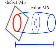
Figure 3: The Lens space $L(k,1)$ is the torus bundle fibered over an interval. Each half of this bundle is a solid torus $T^{2}\times I_{L,R}$. The M5-brane on the whole Lens space gives the gauge group $U(1)_{k}$ and the defect M5-brane leads to matter and the flavor symmetry $U(1)$. In this Figure, we put the defect M5-brane on the left endpoint, which could move to the right endpoint; see Figure 4. In addition, the red circle as the intersection is matter circle.

M-theory/IIB duality. Let us recall the tool, which is the duality between M-theory and IIB string theory. The duality applies on the spacetime

$$\mathbb{R}_{12}^{2}\times S_{0}^{1}\times N_{345}\times L(k,1)_{69\sharp}\times\mathbb{R}^{2}_{78}\,,$$ (28)

where we have assigned coordinates on all directions. The elliptic fiber bundle reads $T^{2}_{9\sharp}\hookrightarrow L(k,1)\rightarrow I_{6}$, where the torus fiber $T^{2}_{9\sharp}=S^{1}_{9}\times S^{1}_{\sharp}$ has longitude $S^{1}_{9}$ and meridian $S^{1}_{\sharp}$. We remind that the identification of meridian and longitude is important, which cannot be switched randomly.

The M/IIB duality is a combination of T- and S-duality in string theories. Basically, the T-duality is between Dp-branes:

$$\text{Dp wrap on }x_{i}\leavevmode\nobreak\ \leavevmode\nobreak\ \xlongleftrightarrow{\text{T-dual on }x_{i}}\leavevmode\nobreak\ \leavevmode\nobreak\ \text{D(p-1) at a point on }x_{i}\,$$

where the direction $x_{i}$ is a direction that Dp-brane extends on. The M-theory and IIB are related through the torus $\text{M}/T_{9\sharp}^{2}\simeq\text{IIB}/S_{9}^{1}$. More specifically,

$$\text{M-theory}\leavevmode\nobreak\ \xrightarrow{\leavevmode\nobreak\ \leavevmode\nobreak\ \text{shrink}\leavevmode\nobreak\ S^{1}_{\sharp}\leavevmode\nobreak\ }\leavevmode\nobreak\ \text{IIA}\leavevmode\nobreak\ \xrightarrow{\leavevmode\nobreak\ \text{T-dual along }x^{9}\leavevmode\nobreak\ }\leavevmode\nobreak\ \text{IIB}\,.$$ (29)

In addition, we need to mention that because of the relation below

$$\frac{l_{p}^{3}}{R_{9}R_{\sharp}}={\tilde{R}_{9}}\,,$$ (30)

the radius of the dual circle in IIB is infinite large $\tilde{S}_{9}^{1}\rightarrow\infty$, as the area of the the torus $\text{Area}\big{(}T^{2}_{9\sharp}\big{)}\simeq R_{9}R_{\sharp}\rightarrow 0$ vanishes at both endpoints of the interval $I_{6}$.

3.1 Defect M5-branes

Using M-theory/IIB string duality and following the discussion in Kitao:1999aa , one can find defect M5-branes lead to $(p,q)$5-branes in IIB string theory, depending on whether M5-branes take the M-theory circle $S^{1}_{\sharp}$ or $S^{1}_{9}$. One can first study brane configurations at one endpoint of the interval $I_{6}\in L(k,1)$. We fix the brane configuration and present it in Table 2. The branes on the other endpoint can be obtained by redefining coordinates through gluing maps. In short, we find the Lagrangian defects should wrap the longitude $S^{1}_{9}$ of $T_{9\sharp}^{2}$ to engineer matters, because only these defect M5-branes are dual to flavor D5-branes, and hence each defect M5-brane corresponds to a hypermultiplet in fundamental representation, which contains two chiral matter F and AF with opposite charges $\pm q$. Interestingly, we notice that the winding number of the defect M5-brane on $S^{1}_{9}$ is the charge $q$ of the chiral multiplet, which matches with the conjecture we draw in section 2.3. In the following, we give detailed analysis.

		$\overbracket{\qquad\qquad}^{S^{1}\times\mathbb{R}^{2}}$			$\overbracket{\qquad\qquad}^{N_{345}}$			$\overbracket{\qquad\qquad}^{I_{6}\times T^{2}_{9\sharp}}$			$\overbracket{\qquad}^{\mathbb{R}^{2}}$
11d	branes	0	1	2	3	4	5	6	9	$\sharp$	7	8
M-theory	$N_{c}$ M5	0	1	2				6	$9_{\text{A}}$	$\sharp$
IIA	$N_{c}$ D4	0	1	2				6	$9_{\text{A}}$
IIB	$N_{c}$ D3	0	1	2				6
IIA	D0									$\sharp$
IIA	D6	0	1	2	3	4	5		$9_{\text{A}}$
IIB	$\text{D}5\xrightarrow{\small S}{\color[rgb]{0,0,1}\text{NS}5}$	0	1	2	3	4	5
M-theory	$\text{M}5^{\prime\prime}$	0	1	2	3	4			${\color[rgb]{1,0,0}9_{\text{A}}}$
IIA	$\text{NS}5^{\prime\prime}$	0	1	2	3	4			$9_{\text{A}}$
IIB	$\text{NS}5^{\prime\prime}\xrightarrow{\small S}{\color[rgb]{1,0,0}\text{D}5}$	0	1	2	3	4			$9_{\text{B}}$
M-theory	$\text{M}2$	0					5		$9_{\text{A}}$
IIB	$\text{D}1\xrightarrow{\tiny{S}}\text{F}1$	0					5
M-theory	$\text{M}5^{\prime}$	0	1	2	3	4				$\sharp$
IIA	$\text{D}4^{\prime}$	0	1	2	3	4
IIB	$\text{D}5^{\prime}\xrightarrow{\small S}\text{NS}5$	0	1	2	3	4			$9_{\text{B}}$
M-theory	$\text{M}2$	0					5			$\sharp$
IIB	$\text{F}1\xrightarrow{\tiny{S}}\text{D}1$	0					5

Table 2: In this table, we show all the necessary branes and their directions. As direction $x_{9}$ appears in both IIA and IIB, we distinguish them by a subscript in $9_{\text{A}}$ and $9_{\text{B}}$ to avoid confusion.

From Lens spaces to 3d brane webs. To begin with, the gauge group is engineered by a single M5-brane wrapping on the whole Lens space $L(k,1)$. It reduces to a D4-brane after shrinking the 11-th circle $S^{1}_{\sharp}$, and T-duality along the meridian $S^{1}_{9}$ of the torus $T^{2}_{9\sharp}$ turns it into a D3-brane in IIB string theory, which gives rise to the gauge group $U(1)$. In short, $\text{M}5(1269\sharp)\rightarrow\text{D}4(1269)\rightarrow\text{D}3(126)$. This process is present in Table 2.

The bare CS level of this gauge group $U(1)_{k}$ is determined by the relative angle between two NS5-branes. These NS5-branes comes from the reduction of D6-branes on two endpoints of the interval $I_{6}\in L(k,1)$, which are magnetic monopoles of D0-branes that are Kaluza-Klein modes of the gravition along $S^{1}_{\sharp}$, and hence D6-branes emerge only at points where the $S^{1}_{\sharp}$ shrinks. For Lens spaces, only at endpoints of the interval $I_{6}$, $S^{1}_{\sharp}$ shrinks and hence D6-branes emerge; see Gukov:2015aa for more discussions. This property of Lens space is nice, as it naturally engineers NS5-branes. Moreover, since D6-branes lead to D5-branes in IIB string theory, S-duality in IIB must be applied to turn these D5-branes into NS5-branes; see Table 2. In short, the process of engineering NS5-branes is $\text{D}0\rightarrow\text{D}6(\text{IIA})\rightarrow\text{D}5(\text{IIB})\xrightarrow{\tiny{S}}\text{NS}5(\text{IIB})$. At the other endpoint of $I_{6}$, another $\text{NS}5^{\prime}$-brane is emerged, which differs from $\text{NS}5$ by a relative angle $\theta$, and the Chern-Simons level yields $k=\tan\theta$, which is also the framing number of $L(k,1)$.

The above construction gives the 3d brane web $\text{NS}5-\text{D}3-\text{NS}5^{\prime}$. We need to check various known brane configuration in Kitao:1999aa to see if this construction is correct. In Kitao:1999aa , there are three ways to break $\mathcal{N}=4$ to $\mathcal{N}=2$ by turning on various relative angles. Fortunately, the 3d brane web we just obtained from Lens space is one of them, which is the case that requires the condition $\rho=\theta$, where $\rho$ and $\theta$ are the relative angles on planes $x_{9\sharp}$ and $x_{59}$ respectively. Because of this particular condition, there is no obvious difference between NS5 and D5, as they only differ by an angle on the plane $x_{59}$. This special case is also the 3d brane webs that can be obtained by Higgsing 5d $\mathcal{N}=1$ brane webs, see e.g.Dimofte:2010tz ; Cheng:2021nex ; Cheng:2021vtq . In IIB-string theory, we should have $\theta=\pi/2$ to distinguish NS5 and D5, which means NS5 is along vertical direction and D5 is along horizontal direction on plane $x_{59}$. Therefore, the $\text{NS}5^{\prime}$-brane should be denoted more precisely by $(k,1)$ 5-brane.

Let us consider the defect M5-brane. The defect $\text{M}5^{\prime\prime}$-brane on $\mathbb{R}_{45}^{2}\times S^{1}_{9}\subset N_{345}\times L(k,1)_{69\sharp}$ leads to a D5-brane via M/IIB duality and S-duality. This D5-brane is responsible for the flavor symmetry and introduces a hypermultiplet. For $L(0,1)$, what we get is a $\mathcal{N}=4$ theory $U(1)_{0}$ with a hypermultiplet. If $k\neq 0$, then $\mathcal{N}=4$ breaks to $\mathcal{N}=2$, and the hypermultiplet can be viewed as a fundamental (F) and an antifundamental chiral multiplet (AF). In plumbing graphs of this note, all AF are decoupled, such as (4). The evolution of the defect brane is

$$\text{M}5^{\prime\prime}(12349)\rightarrow\text{NS}5(12349)(\text{IIA})\rightarrow\text{NS}5(12349)(\text{IIB})\xrightarrow{S}\text{D}5(12349)(\text{IIB})\,.$$

For this defect, the intersection is the longitude $\text{M}5\cap\text{M}5^{\prime\prime}=S^{1}_{9}$. This defect brane is suitable for engineering matter since the M2-branes also agree with strings in 3d brane webs.

Now, we can try to find mass or FI parameters. Recall that the length of the F1 strings between the D3 and D5 is the real mass parameter, while that of D1-branes between D3 and NS5 is the FI parameter. F1 and D1 can be exchanged through S-duality. Since defect M5 and bulk M5 are separated along direction $x_{5}$, the M2-brane should stretch between these two M5-branes, and one of its boundaries is the intersection $\partial(\text{M}2)=\text{M}5\cap\text{M}5^{\prime}=S^{1}_{9}$, and the other boundary is the extension of $S^{1}_{9}$ into the fiber. The M2-brane should be a cylinder on direction $x_{59_{\text{A}}}$, namely $I_{5}\times S^{1}_{9}$. The M2-brane descends $\text{M}2(59)\rightarrow\text{D}2(59)\xrightarrow{T_{9}}\text{D}1(5)\xrightarrow{S}\text{F}1(5)$ under dualities. The mass parameter as the coordinate $m=x_{5}$ takes values from $(-\infty,+\infty)$. If the matter is massless, then $m=x_{5}=0$. Note that when $S^{1}_{9}\rightarrow 0$, the matter has to be massless.

We need to remind that because of the relation (30), at a generic point on the interval $I_{6}$ the fiber torus has a non-vanishing area; therefore, the D5-brane introduced by defect is a loop on $S^{1}_{9_{\text{B}}}$ with finite radius. Only when this defect is moved to endpoints, the radius of this loop becomes infinite large.

One can also consider the defect $\text{M}5^{\prime}$ along the meridian $S^{1}_{\sharp}$. However, if we perform S-duality, then $\text{M}5^{\prime}(1234\sharp)\rightarrow\text{D}5^{\prime}(12349)\xrightarrow{S}\text{NS}5(12349)$, which unfortunately is not a D5 and hence this $\text{M}5^{\prime}$ is not very suitable for engineering matters, although there is an exception; see (52). The M2-brane between the bulk M5 and defect $\text{M}5^{\prime}$ is finally turned into a D1-brane: $\text{M}2(5\sharp)\rightarrow\text{F}1(5)\xrightarrow{T_{9}}\text{F}1(5)\xrightarrow{S}\text{D}1(5)$. The topology of this M2-brane is the cylinder $I_{5}\times S^{1}_{\sharp}$, and hence the distance $I_{5}$ engineers the FI parameter. Note that at endpoints of $I_{6}$, $S^{1}_{\sharp}$ shrinks and hence FI parameter always vanishes.

FI parameters. FI parameter in principle should be independent of the defect M5-brane as it is given by the D1-string stretching between D3 and NS5. Unfortunately, we have not clearly identify the FI parameter, but only find two candidates. Both candidates suggest $S^{1}_{9}$ is responsible for the FI parameter.

In M-theory, FI parameter is usually known as the volume of the M2-brane ending on the bulk $\text{M}5$ in e.g. Ooguri:1999bv . For Lens spaces, there is naturally a circle $S^{1}_{9}$ which does not shrinks. For this candidate, the topology of this M2-brane is a disc with $S_{9}^{1}$ as its boundary, and the bulk of M2 extends to the Lens space.

We have another candidate for FI parameter. The massless M2-brane taking $T^{2}_{9\sharp}$ can be inserted in the volume of the bulk M5-brane. Note that this M2-brane does not have a boundary. However, because of the existence of the D0-brane, there should be a subtle interaction that traps this M2-brane at the volume of the bulk M5-brane. This M2-brane $\text{M}2(09_{\text{A}}\sharp)$ leads to $\text{F}1(09_{\text{A}})$ in IIA and then is T-dual to $\text{F}1(09_{\text{B}})$ in IIB. After S-duality, this F1 becomes a $\text{D}1(9_{\text{B}})$. Once again, because of the M/IIB duality, the radius of $S_{9_{\text{B}}}^{1}$ opens up and hence is infinite large. This $\text{D}1(9_{\text{B}})$ would be appropriate to engineer the FI parameter, because in 3d brane webs, D3 and NS5 locate at two separate points on the direction $x_{9_{\text{B}}}$ and the distance between them is FI parameter. We can also use IIA to track D3 and NS5. The M5-brane system reduces to $\text{D}4-\text{D}6$ with the intersection being $S^{1}_{9_{\text{A}}}$ wrapped by $\text{F}1(9_{\text{A}})$, namely $\text{D}4\cap\text{D}6=\text{F}1$. After the T-duality along $S^{1}_{9_{\text{A}}}$, $\text{D}4\rightarrow\text{D}3$ and $\text{D}6\rightarrow\text{NS}5$, and the D3 can be deformed away from NS5 along $x_{9_{\text{B}}}$. Note that this F1 string is given by the M2-brane in the volume of M5-brane, so it is a self-dual string.

Charges and (p,q)-branes. In Kitao:1999aa , it is discussed that the generic defect M5-brane can wrap $q$-times on $S^{1}_{9}$. This M5-brane could lead to a charge-$q$ NS5-brane, which under S-duality becomes a charge-$q$ D5-brane. This charge-$q$ D5-brane suggests a 3d brane web $\text{D}3(6)-\text{NS}5(5)-\text{D}5^{q}(9)$, which engineers a charge-$q$ matter. After S-duality the D1(5) becomes F1(5), which provides $q$ Higgs vacua for the D3 to end on the charge-$q$ D5-brane. These $q$ vacua are points that were evenly distributed on $S^{1}_{\sharp}$, which separate the charge $q$ D5-branes into $q$ fractions as shown in Figure 5. The relative real mass parameters between D5-brane fractions are $m_{i}\sim S^{1}_{\sharp}/q$. Since $S^{1}_{\sharp}$ shrinks on endpoints of $I_{6}$, these fractions coincide to an overlapped charge-$q$ D5-branes on endpoints. There is still an overall mass parameter $m_{0}$ left, which is the length of the F1(5) string along $x_{5}$.

Moreover, if a M2-brane wraps $q$ times on $S_{9}^{1}$ and $p$ times on $S_{\sharp}^{1}$, then one can get a $(p,q)$-string along $x_{5}$ in IIB. Generically, a defect M5-brane wrap $(q,p)$ times on $T_{9_{\text{A}}\sharp}^{2}$ leads to a $(p,q)5$-brane along $x_{12349_{\text{B}}}$, Once again, the brane configuration shows that the charges should be winding numbers, which agrees with what we have learned from handle-slides in section 2.

Gluing maps and charge-$q$ defects. The bare CS level $k$ is enigneered by the self-twisting/framing number of the Lens space $L(k,1)$. Its definition is slightly different from linking numbers, which needs the information of gluing maps between two solid tori. We can denote $S_{\sharp}^{1}$ and $S_{9}^{1}$ by meridian $\alpha$ and longitude $\beta$ for later convenience, which are gauge circle and matter circle respectively. These two circles are transformed by the gluing map which is an element in the mapping class group $SL(2,\mathbb{Z})$. The gluing map $f:\,T^{2}\rightarrow T^{2}$ is represented as a matrix:

$$\begin{bmatrix}\tilde{\alpha}\\ \tilde{\beta}\end{bmatrix}=\begin{bmatrix}k&1\\ -1&0\end{bmatrix}\cdot\begin{bmatrix}{\alpha}\\ {\beta}\end{bmatrix}\,.$$ (49)

The framing number is defined as $k:=\beta\cdot\tilde{\alpha}$, which is the linking number between longitude and the deformed meridian. However, in terms of circle/surgery representation of Lens spaces in section 2.3, in particular the $\beta$-type Kirby moves, it is more natural to use the self-intersection notation, namely $L\cdot L:=\beta\cdot\tilde{\beta}=k$. These two definitions match, as surgery is gluing back a solid torus to a torus hole, so the meridian and longitude should be switched.

The charge-$q$ matter circle is the multiple winding of the charge-$1$ matter circle, so it is given by ${\beta}_{q}=q\,\beta$. One can check that the intersection/linking numbers between the gauge and matter circles are not changed by the gluing map, namely $\alpha_{q}\cdot\beta=\tilde{\alpha}_{q}\cdot\tilde{\beta}=q$, since $\alpha\cdot\alpha=0\,,\leavevmode\nobreak\ \beta\cdot\beta=0\,,\leavevmode\nobreak\ \alpha\cdot\beta=1$.

3d theory on $S^{1}\times\text{annulus}$. One can consider a trivial three-manifold $T^{2}\times I$, where the torus never degenerates on the interval $I$. This geometry can be obtained from $S^{2}\times S^{1}$ by truncating two poles of $S^{2}$. For this geometry, since no $S^{1}$ degenerates, one can not get D6-branes. Fortunately, one can add defect M5-branes on meridian and longitudes of $T^{2}$ to get NS5-branes and D5-branes respectively. This geometry is useful, as it can be used to connect Lens spaces. We will go back to this geometry in section 4.3.

3.2 Brane webs on torus

Movement of D5-branes. The movement of D5-brane in Cheng:2021vtq can be described by gluing maps in (49). At the other endpoint of $I_{6}$, the $S_{9}^{1}$ and $S^{1}_{\sharp}$ are mapped to $\tilde{S}_{9}^{1}$ and $\tilde{S}^{1}_{\sharp}$ where $\tilde{S}_{9}^{1}=-S^{1}_{9}$ and meridian $\tilde{S}_{\sharp}^{1}=kS^{1}_{9}+S^{1}_{\sharp}$, so the $S_{9}^{1}$ is reversed and $S_{\sharp}^{1}$ is twisted. This suggests the transformations of various 5-branes.

The bulk M5-brane on Lens space $L(k,1)$ leads to the $\text{NS}5-\text{D}3-(k,1)\text{5-brane}$ web, where the NS5 and $(k,1)5$-brane are differed by a relative angle $k=\tan\theta$. We can undo the S-duality to return $\text{D}5-\text{D}3-(1,k)\text{5-brane}$. Note that in addition to generate $(1,k)\text{5-brane}$ from a D6-brane, it can also arise from a defect M5-brane wrapping $\tilde{S}_{\sharp}^{1}=kS^{1}_{9}+S^{1}_{\sharp}$; see Table 2.

The flavor $\text{D}5$ brane given by the defect M5 is almost invariant under the gluing map, as $\tilde{S}_{9}^{1}=-S_{9}^{1}$ only reverses the charge. This means that if we move a D5-brane from one endpoint of $I_{6}$ to the other endpoint, we still get the same D5-brane only with its orientation reversed, namely the signs of charges for 3d chiral multiplets are shifted. This is consistent with the already known fact from 3d brane webs in IIB string theory Cheng:2021vtq . We use the Figure 4 to illustrate this parallel movement of the defect M5-branes/D5-branes. Before and after the move, the defect M5 always gives rise to the same pair of chiral multiplets. Note that the red line (D5-brane) gives a hypermultiplets, or in other words, a pair of chiral multiplets $1\textbf{F}+1\textbf{AF}$, change to $1\textbf{AF}+1\textbf{F}$, once they are moved to the other endpoint.

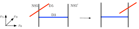
Figure 4: The movement of a D5-brane in the 3d brane web. After the movement, the orientation of D5-brane is reversed, which switches the charges of chiral multiplets.

Some Lens space chould also engineer abelian 3d $\mathcal{N}=4$ theories, as they differ to 3d $\mathcal{N}=2$ theories only by turning off Chern-Simons levels. We can let the bare Chern-Simons level vanishing, then $\text{NS}5^{\prime}=\text{NS}5$ and the Lens space is only $L(0,1)=S^{1}\times S^{2}$. To get the theory $\bullet_{k}-{\color[rgb]{.5,.5,.5}\blacksquare}$ with only one ${\color[rgb]{.5,.5,.5}\blacksquare}$, the matter AF should be decoupled by sending its mass $m_{a}\rightarrow-\infty$. More explicitly, since the effective Chern-Simons level is $k_{\text{eff}}=k+\big{(}N_{f}\text{sign}(m_{f})-N_{a}\text{sign}(m_{a})\big{)}/2$, for the theory $U(1)_{0}+N_{f}\textbf{F}+N_{a}\textbf{AF}$, one should let two matters in the theory $U(1)_{0}+1\textbf{F}+1\textbf{AF}$ to have opposite signs, namely $\text{sign}(m_{f})\text{sign}(m_{a})<0$, such that eventually $k_{\text{eff}}=\pm 1$ to produce the basic building block $U(1)_{\pm 1}+1\textbf{F}$, which is required for constructing plumbing theories through $ST$-moves. It is already known how to perform decoupling and give opposite signs to both matters on 3d brane webs in IIB, while on the M-theory it is unclear. The patterns of various decoupling are discussed in Cheng:2021vtq . In below, we present the 3d brane web for $U(1)_{0}+1\textbf{F}+1\textbf{AF}$ and its decoupled brane webs for plumbing graph $\bullet_{+1}-{\color[rgb]{.5,.5,.5}\blacksquare}$. If we look at the brane webs along direction $x_{6}$, they take the following forms

(50)

The 3d brane webs for $U(1)_{\pm 1}$ with a D5-brane can also decouple to $\bullet_{\pm 1}-{\color[rgb]{.5,.5,.5}\blacksquare}$. We briefly draw brane webs below to illustrate:

(51)

The 3d brane web for $U(1)_{\pm 1}$ with a NS5-defect is special, as it also finally leads to $\bullet_{\pm 1}-{\color[rgb]{.5,.5,.5}\blacksquare}$. We illustrate transformations of its brane webs below

(52)

From $(a)$ to $(b)$, we apply S-duality, and from $(b)$ to $(c)$ we just change the slope of $(b)$ using $SL(2,\mathbb{Z})$ transformation of IIB string theory, which turns $(p,\pm 1)$-brane to $(p+n,\pm 1)$-brane, but preserves $(\pm 1,0)$-brane. The $(c)$ or its equivalent web $(d)$ are the brane web for the theory $T[U(1)]\oplus 1\text{D}5$, where $T[U(N)]$ is the self-dual theory in Gaiotto:2008ak . Obviously, if further applying S-duality on $(d)$, one gets the theory $U(1)_{0}+1\textbf{F}+1\textbf{AF}$. Similarly, one can also draw the brane webs for $U(1)_{1/n}\oplus 1\text{NS}5$ for any $n\in\mathbb{Z}$, which always end up with the same web $(d)$. Thus, for this particular theory $U(1)_{1/n}$, the defect along $S^{1}_{\sharp}$ can also be used to introduce chiral multiplets, although this defect leads to a $\text{NS}5$. This phenomenon is analogous to the properties of Lens space $L(1,n)=S^{3}$ that we will discuss in section 4.2, and leads to an exceptional case of defects that engineer matters.

Brane webs on torus. In this subsection, we discuss the winding patterns of the defect M5-branes on $T_{9\sharp}^{2}$. We find that on this torus, one can equivalently analyze its dual 3d brane webs, which even suggests new 3d brane webs.

Wrapping a defect M5-brane $q$-times on longitude $S^{1}_{9}$ and $p$-times on meridian $S^{1}_{\sharp}$ leads to a charge $(p,q)$ 5-brane along $(12349_{\text{B}})$, see e.g. Kitao:1999aa . After S-duality in IIB, this 5-brane becomes a $(q,p)$ 5-brane. One can take a quotient $\mathbb{Z}_{q}$ on torus to reproduce this winding number/charge $q$. We illustrate this in Figure 5.

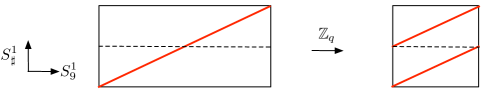
Figure 5: In this example, the $q=2$. The charge $q$ equals to the number of components along meridian $S^{1}_{\sharp}$. The red line is the circle wrapped by the defect M5. The quotient of circles is $S_{\sharp}^{1}\rightarrow S^{1}_{\sharp}\,,\leavevmode\nobreak\ S_{9}^{1}\rightarrow qS_{9}^{1}$.

If we put a defect $(1,1)$, then the quotient makes it to $(q,1)$.

Recall that the D6-brane comes from D0-brane on $S^{1}_{\sharp}$, which can be represented as a vertical line on the torus. Then circles corresponding to a NS5 and a charge $q$ D5 are given by

$$\centering\begin{split}\includegraphics[width=57.81621pt]{figgeo/qcircle.pdf}\end{split}\@add@centering$$ (53)

On this torus, the vertical and horizontal lines do not represent the same type of branes, so it is more better to consider the dual IIB configuration to see if these lines can be combined into other branes. In the IIB, if a NS5 meets an charge $q$ D5, then one can split the D5 into two half-infinite lines, and each half-infinite line gives to a chiral multiplet of charge $q$ or $-q$, depending on their positions. If one decouples both matters, then the slope of the NS5 is shifted by the formula (5):

$$\Delta k=\tan\theta=\frac{q^{2}}{2}\text{sign}(m_{\textbf{F}_{q}})-\frac{q^{2}}{2}\text{sign}(m_{\textbf{AF}_{-q}})\,.$$ (54)

Therefore, every time when a NS5 meets a charge $q$ component, the merged 5-brane picks up an additional charge $(q,0)$ because of the charge conservation. There are $q$ fractions, and hence the $\text{NS}5$ is finally becomes a $(q^{2},0)$-brane:

$$\centering\begin{split}\includegraphics[width=122.85876pt]{figgeo/chargqweb1.pdf}\end{split}\@add@centering$$ (55)

In particular, $\Delta k=\pm q^{2}$ if $\text{sign}(m_{\textbf{F}_{q}})\cdot\text{sign}(m_{\textbf{AF}_{-q}})=-1$, and $\Delta k=0$ if $\text{sign}(m_{\textbf{F}_{q}})\cdot\text{sign}(m_{\textbf{AF}_{-q}})=+1$.

We are interested in the Lens space $L(0,1)$ with a charge $q=+1$ matter and $\Delta\theta=\pm\pi/4$, as this theory gives to $\bullet_{+1}-{\color[rgb]{.5,.5,.5}\blacksquare}$ after decoupling the AF which shifts the slope of NS5 to $\text{NS}5^{\prime}$ as follows:

$$\centering\begin{split}\includegraphics[width=108.405pt]{figgeo/depqD5.pdf}\end{split}\@add@centering$$ (56)

Correspondingly, the slope of the shrinking circle $S^{1}_{\sharp}$ wrapped by D0 should also be shifted from $S_{\sharp}^{1}\rightarrow S_{\sharp}^{1}\pm S_{9}^{1}$; then this quantum correction transforms $L(0,1)$ into $L(\pm 1,1)$. It is a geometric transformation when a defect M5 (denoted as $L_{\color[rgb]{1,0,0}{\bigcirc}}$) is present:

$$S^{1}\times S^{2}\sqcup L^{\prime}_{\color[rgb]{1,0,0}{\bigcirc}}\leavevmode\nobreak\ \xrightarrow{\text{decoupling {AF}}}\leavevmode\nobreak\ S^{3}\sqcup L_{\color[rgb]{1,0,0}{\bigcirc}}\,,$$ (57)

which gives effective CS levels $k_{\text{eff}}=\pm 1$. Moreover, instead of decoupling both chiral multiplets, we can also only decouple AF by taking $m_{a}\rightarrow-\infty$ and keep F, however, this does not change $k_{\text{eff}}$ as F is assumed to have a positive mass in the renormalization; see Tong’s lectures Tonglec for a nice discussion. The effective CS levels are naturally selected by plumbing graphs, as we have shown in (21). This geometric change caused by decoupling is analogous to the handle-slide, although the latter may contain more information. After the Dehn twist or decoupling, the framing number describing effective CS levels changes significantly $\bullet_{k}\rightarrow\bullet_{k+q^{2}}$.

3.3 3d theories from Lens spaces.

In this subsection, we look at the theories that can be engineered by Lens spaces. Firstly, it is free to add many defect M5-branes on Lens spaces $L(k,1)$. These M5-branes can only be parallel to each other, as the longitude $S^{1}_{9}$ is unique for Lens spaces. However, we can distinguish them by tuning on different mass parameters $m_{i}$ and winding numbers $q_{i}$. Thus Lens spaces with Lagrangian defects can engineer the class of theories:

$$U(1)_{k}+\oplus_{i=i}^{N_{f}}\textbf{F}_{q_{i}}+\oplus_{i=i}^{N_{a}}\textbf{AF}_{q^{\prime}_{i}}\,,$$ (58)

where $N_{f}$ is the number of defect M5-brane, and charge $q_{i}$ are the winding numbers of defect M5-branes on the matter circle $S^{1}_{9}$. For instance, one can introduce two matters, and the configuration of putting two defects on the same solid torus is

$$\centering\begin{split}\includegraphics[width=144.54pt]{figgeo/twoFtorus.pdf}\end{split}\@add@centering$$ (59)

It is obvious that when matter circles coincide, Lagrangian defects coincide as well and the flavor symmetry is enhanced to $U(N_{f})$. This fusion of defects is interesting, and we leave it for future work.

The matter circle and gauge circle can be easily identified, as they are longitude $S^{1}_{9}$ and meridian $S_{\sharp}^{1}$ on torus respectively. We can use the following figure to illustrate the transport of these two circles from one endpoint to the other:

$$\centering\begin{split}\includegraphics[width=216.81pt]{figgeo/mcircle.pdf}\end{split}\@add@centering$$ (60)

If we cut the $I_{6}$ in the middle, then the left part is a solid torus $D^{2}\times S^{1}_{9}$, so the transport (movement) of matter circles is the deformation of circles from the core to bulk of the solid torus. The theory is totally determined by defects and the gluing map which fixes the framing numbers $k$.

The matte circle can be viewed as the flavor D5, and gauge circle can be viewed as the NS5. Since NS5 can transports and gets twisted, the D3-brane could suspend in between and provides the space for deformation and gluing. This is why we call it gauge circle. The correspondence between the solid torus and the part of 3d brane web is:

$$\centering\begin{split}\includegraphics[width=108.405pt]{figgeo/torusbrane.pdf}\end{split}\@add@centering$$ (61)

Notice that the D3-brane has a finite length $I_{6}$, as its gauge coupling is finite. The gauging of D3-brane is given by gluing two solid tori.

4 Surgery constructions of matters

In the last section, we analyzed Lens spaces $L(k,1)$. However, Lens spaces can only engineer theories with one gauge node $U(1)_{k}$, and hence are not generic. The generic three-manifolds are constructed by Dehn surgeries on links of circles (plumbing graphs). In this section, we will discuss how to introduce defect M5-branes through Dehn surgeries, and see how they interact with gauge groups.

4.1 Dehn surgeries and $ST$-moves

Lens spaces are building blocks of any closed orientable three-manifolds, namely

$$M_{3}=L(k_{1},1)\sqcup L(k_{2},1)\sqcup\cdots\sqcup L(k_{n},1)\,,$$ (62)

for which the circles $L_{i}$ for Lens spaces are linked with each other, and the link $L_{1}\cup L_{2}\cup\cdots\cup L_{n}$ could represent the $M_{3}$. Recall that plumbing graphs denote this link by the rules that $L_{i}\rightarrow\bullet_{k_{i}}$ and $L_{i}\cup L_{j}\rightarrow\bullet_{k_{i}}-\bullet_{k_{j}}$. Equivalently, $M_{3}$ is defined as Dehn surgeries along these links

$$M_{3}:=S^{3}\backslash N(L_{1}\cup L_{2}\cup\cdots\cup L_{n}):=\left(S^{3}-\cup_{i=1}^{n}N(L_{i})\right)\leavevmode\nobreak\ \sqcup_{f_{i}}\leavevmode\nobreak\ \left(\oplus_{i=1}^{n}D_{i}^{2}\times S^{1}\right)\,.$$ (63)

The definition of Dehn surgery is illustrated in Figure 1, which is the process of drilling out the neighborhood of the circle $L_{i}$, namely $N(L_{i})=D_{i}^{2}\times L_{i}$, and then filling in a solid torus $D_{i}^{2}\times S^{1}$. The knot complement $S^{3}-N(L_{i})$ is called knot exterior, whose boundary is a torus even if the $L_{i}$ is knotted. We need to glue back a solid torus $D^{2}\times S^{1}$ by the gluing map ${f}_{i}$ to each torus hole. Note that these solid tori $D_{i}\times S^{1}$ are independent.

The Dehn surgery says that the gluing map $f_{i}$ is determined by the meridian $\alpha_{i}$ of the solid torus and the curve $J_{i}$ on the boundary of the complement $S^{3}-N(L_{i})$, namely $f_{i}(\alpha_{i})=J_{i}$. Therefore, the gauge circle as the meridian $\alpha_{i}$ is analogous to the circle $L_{i}$. Moreover, the Dehn surgery for Lens spaces differs from gluing two solid tori by the torus switch which is defined as exchanging meridian and longitude ${\alpha_{i}}\leftrightarrow{\beta_{i}}$. Therefore the gluing map (49) is transposed and the images of meridian of longitude of solid torus $D^{2}\times S^{1}$ are

$$\begin{bmatrix}\tilde{\alpha}\\ \tilde{\beta}\end{bmatrix}=\begin{bmatrix}k&-1\\ 1&0\end{bmatrix}\cdot\begin{bmatrix}{\alpha}\\ {\beta}\end{bmatrix}\,.$$ (64)

The longitude $\beta$ represents circle $L$, and the Jordan curve is $J=k\alpha-\beta$. The framing number is defined as $L\cdot L:=\beta\cdot J=k$.

$ST$-moves and matter circles. In the last section, using M-theory/IIB duality we find matter nodes on plumbing graphs do indeed exist and should be the matter circles given by defect M5-branes, and the charge $q$ of the matter is the winding number between gauge circle and matter circle. Therefore, one can draw the link graph below for the simple plumbing theory:

$$\centering\begin{split}\includegraphics[width=108.405pt]{figgeo/hopfplumb.pdf}\end{split}\@add@centering$$ (65)

Matter circle and gauge circle should form a Hopf link in each solid torus (61). We apologize that the colors of link graphs and plumbing graphs do not match. One can add many matter nodes on the same gauge node, then correspondingly, many matter circles (red circle) should link to the gauge circles (blue circle). Changing the orientation of red circles flips the signs of charges.

Note that at this stage the matter circle ${\color[rgb]{1,0,0}{\bigcirc}}$ is just a circle given by the intersection of Lagrangian defect with three-manifolds. Thus one cannot apply Dehn surgery on the matter circle. However, in section 4.4, we will show that matter circle relates to the three-sphere $S^{3}_{\infty}$.

Because of the mirror duality in (2), the matter circle can be equivalently viewed as a decorated gauge circle $\bullet_{+1}-{\color[rgb]{.5,.5,.5}\blacksquare}$, on which one can apply Dehn surgery. To see the topology, one can represent the $ST$-moves by matter circles and gauge circles. For instance, the $ST_{\alpha}$-move with $q=1$ (13) is represented as

(66)

which is a non-trivial replacement. In section 4.4, we will try to geometrically derive this $ST_{\alpha}$-move. We draw the matter circle (red) big on the left graph and small on the right graph. This is due to the mirror map. The FI parameter $\xi$ of the gauge circle $U(1)$ is mirror dual to the mass parameter $m$ of the matter F, and we assume the length of ${\color[rgb]{0,0,1}{\bigcirc}}$ is the FI parameter. In addition, it is shown by sphere partition functions of this mirror triality in Cheng:2023ocj that the matter in dual theory $\bullet_{\pm 1}-{\color[rgb]{.5,.5,.5}\blacksquare}$ is almost massless up to a quantum shift $q^{*}=e^{i*\epsilon}$. Therefore, in (66) we can draw the scales of matter circles by the values of parameters.

According to Lickorish-Wallace theorem, any closed orientable three-manifold can be obtained by Dehn surgeries along a link in $S^{3}$, and each component of this link can be an unknot $\bigcirc$. This means that if a three-manifold is given by surgeries along a knot, then this knot can be equivalently replaced by links of circles using Kirby moves. In principle, all 3d plumbing theories in Cheng:2023ocj can be engineered by links and defects. One example has been shown in Figure 2. Here we illustrate a knot example in Figure 6.

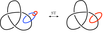
Figure 6: This three-manifold is given by the Dehn surgery along a trefoil in $S^{3}$. The winding number between the blue circle ${\color[rgb]{0,0,1}{\bigcirc}}$ and trefoil is the charge $q$ for the matter. Here we insert a matter circle at a simple position such that it does link to the trefoil in a complicated pattern.

In the above, we show fundamental matter circles carried by each solid torus $D^{2}_{i}\times S^{1}$ can bring matters to plumbing manifolds by surgeries. However, these are just a small sector. There could be matters charged under many gauge nodes, such as bifundamental chiral multiplets, trifundamental, and so on, depending on how matter circles are linked with gauge circles. Multi-charged matters cannot be inherited from the fundamental matters on each Lens space component in (62). From the perspective of $\beta$-Kirby moves in (22), these matters with many charges are not basic, and the most basic one is $\bullet_{\pm 1}-{\color[rgb]{.5,.5,.5}\blacksquare}$. In the following, we analyze these matter circles to show their existence.

If a matter node connects to many gauge nodes, then the plumbing theories contains a chiral multiplet with charges $q_{i}$ under gauge groups $U(1)_{k_{i}}$. In the link graph, one just need to link this matter circle to these gauge circles. For example, a bifundamental matter is represented by the following graph

$$\centering\begin{split}\includegraphics[width=144.54pt]{figgeo/bifundcircle.pdf}\end{split}\@add@centering$$ (67)

To engineer bifundamental matter circles in three-manifolds, one can either directly insert a matter circle like (67), or introduce a disconnected gauge circle with a matter $\bullet_{\pm 1}-{\color[rgb]{.5,.5,.5}\blacksquare}$ through the handle-slide in (22), and then perform $ST_{\alpha}$-moves (66) to replace this gauge circle by the matter circle. These two ways lead to the same theories.

4.2 Images of matter circles

For the surgery construction of 3d theories, both gauge circles and matter circles are useful. As we have reviewed in section 4.1, the images of meridians $\alpha_{i}\mapsto J_{i}$ explicitly determine the three-manifolds. One can guess that the images of the longitude $\beta_{i}$ may determine matters. However, the answer is complicated. In this section, we discuss Lens spaces to partly solve this problem. We find various properties of matter circles can be confirmed by 3d brane webs in section 3.2.

Lens spaces ${L(k,1)}$. The Lens space is given by $S^{3}\backslash N(\bigcirc_{k}):=S^{3}-N(\bigcirc)\cup_{f_{k}}(D^{2}\times S^{1})$, where the circle complement $S^{3}-N(\bigcirc)$ has a torus (cusp) boundary. We denote its meridian and longitude by $(\alpha^{\prime},\beta^{\prime})$. The meridian and longitude of the solid torus are $(\alpha,\beta):=((S^{1},*),(*,S^{1}))\subset D^{2}\times S^{1}$ where $*$ means a point on $D^{2}$ or $S^{1}$.

The gluing map $f:(\alpha,\beta)\mapsto(\alpha^{\prime},\beta^{\prime})$ is from the boundary of solid torus to the cusp boundary. For convenience, we denote $\text{Im}(\alpha)=f(\alpha)$ and $\text{Im}(\beta)=f(\beta)$. Then we have

$$\begin{bmatrix}f(\alpha)\\ f(\beta)\end{bmatrix}=\begin{bmatrix}p&-q\\ r&s\end{bmatrix}\cdot\begin{bmatrix}\alpha^{\prime}\\ \beta^{\prime}\end{bmatrix}\,,$$ (68)

where the determinant of the matrix should be one, namely $ps+qr=1$ (unitary condition). The Jordan curve is $J=\text{Im}(\alpha)=p\alpha^{\prime}-q\beta^{\prime}$.

For integral surgeries $L(k,1)$, we have $p=k,q=1$, so $r=-sk+1$ for any $s\in\mathbb{Z}$ could satisfy the unitary condition, which gives infinite many equivalent gluing maps. The images of gauge and matte circle on the cusp torus read

$$f(\alpha)=k\alpha^{\prime}-\beta^{\prime}\,,$$ (69)

$$f(\beta)=(-sk+1)\alpha^{\prime}+s\beta^{\prime}=\alpha^{\prime}-s(k\alpha^{\prime}-\beta^{\prime})=\alpha^{\prime}-sf(\alpha)\,.$$

Note that the framing number is defined as the linking number between the image of meridian and the longitude of cusp torus, namely $f(\alpha)\cdot\beta^{\prime}=k$. One can see that the image of matter circle $\text{Im}(\beta)$ contains Dehn twists of the image $f(\alpha)$. We should set $s=0$ to fix this free integer, and then $f(\beta)=\alpha^{\prime}$ leads to a D5-brane. Otherwise, D5-brane on one endpoint would become a charge $(-sk+1,s)$ 5-brane on the other endpoint. The matter D5-brane should be invariant under this transport as shown in Figure 4.

In short, $(f(\alpha),f(\beta))=(k\alpha^{\prime}-\beta^{\prime},\alpha^{\prime})$. The image of matter circle $\beta$ is fixed and is always the meridian $\alpha^{\prime}$ of the cusp torus. This is consistent with the circle graph in (65). However, there is a special case for $f(\beta)$. When $s=\pm 1$ and $k=\pm 1$, the image of matter circle is $f(\beta)=\pm\beta^{\prime}$. This means that a D5-brane transforms to a NS5-brane. This is the exceptional 3d brane web in (52), which also gives $\bullet_{\pm 1}-{\color[rgb]{.5,.5,.5}\blacksquare}$ after decoupling the AF. In this sense, $L(\pm 1,1)$ are quite special, as both $\alpha^{\prime}$ and $\beta^{\prime}$ can be matter circles.

The integer $s$ can also be fixed from another perspective. Note that the linking number of gauge and matter images is $f(\alpha)\cdot f(\beta)=2sk-1$. It is natural to set $s=0$, such that $f(\alpha)\cdot f(\beta)=-1$, which could ensure that matter circle has winding number $\pm 1$ with gauge circle. Since the winding number is the charge of matter, it should be preserved. For $L(\pm 1,1)$, we can also have $f(\alpha)\cdot f(\beta)=1$ if $s=\pm 1$.

Three-sphere $\mathbf{S^{3}}$. For $L(1,0)=S^{3}_{\infty}$, the meridian of solid torus $\alpha$ maps to $J=\alpha^{\prime}$ of the boundary torus of $S^{3}-N(\bigcirc)$, and the longitude $\beta$ maps to $r\alpha^{\prime}+\beta^{\prime}$. In short,

$$(f(\alpha),f(\beta))=(\alpha^{\prime},r\alpha^{\prime}+\beta^{\prime})\,.$$ (70)

$L(1,0)$ defines the identical/trivial surgery along the circle $\bigcirc_{\infty}$, which is obtained by filling in the same solid torus that was drilled out, so $(\alpha,\beta)\mapsto(\alpha^{\prime},\beta^{\prime})$, which fixes $r=0$. In addition, although it is an identical gluing, if taking into account the torus switch, we have $\text{NS}5\rightarrow\text{D}5$ and the defect $\text{D}5\rightarrow\text{NS}5$. This gives a $U(1)_{0}+1\textbf{F}+1\textbf{AF}$, but the role of NS5 and D5 are flipped. We use the brane web below to illustrate:

(71)

Therefore, identical surgery also leads to the exceptional brane web, which describes the $T[U(1)]$ theory with a D5-brane as shown in (52).

Note that $L(1,n)$ for any $n\in\mathbb{Z}$ give the same three-sphere $S^{3}$. One can understand $L(1,n)$ by thinking about how to obtain it. This $n$ is the number of Dehn twists that send $\alpha^{\prime}=\alpha^{\prime\prime}+n\beta^{\prime\prime}\,,\beta^{\prime}=\beta^{\prime\prime}$ which lead to equivalent surgeries Rolfesn:1984 . Using the unitary condition and taking this twist into (70), we get the images of gauge circle $\alpha$ and matter circle $\beta$ below

$$f(\alpha) =\alpha^{\prime\prime}+n\beta^{\prime\prime}\,,$$ (72)

$$f(\beta) =r\alpha^{\prime\prime}+(rn+1)\beta^{\prime\prime}=r(\alpha^{\prime\prime}+n\beta^{\prime\prime})+\beta^{\prime\prime}=\beta^{\prime\prime}+rf(\alpha)\,,$$

where $(\alpha^{\prime\prime},\beta^{\prime\prime})$ are circles on the cusp boundary of $L(1,n)$. Once again, the image of matter circle contains the $r$-twists of the image of meridian. Just like Lens space $L(k,1)$, we can use the linking number $f(\alpha)\cdot f(\beta)=2nr+1$ to fix $r$ and $n$. It is better to set $r=0$, such that we always have $f(\beta)=\beta^{\prime\prime}$ for any $n$. Another way to understand this $r$-integer is the Dehn twists of $\beta^{\prime}$ along $\alpha^{\prime}$, namely $\beta^{\prime}=\beta^{\prime\prime}+t\alpha^{\prime\prime}\,,\alpha^{\prime}=\alpha^{\prime\prime}$, which could cancel this freedom $r$-integer in (70) by setting $t=-r$, and then this returns $L(1,0)$.

The brane web for $L(1,n)$ are similar to webs in (52), where the matter circle $\text{D}5$ on the endpoint of D3-brane is mapped also to a $\text{NS}5$ on the other endpoint of D3. If $n=\pm 1$, $r=\mp 1$, then $f(\alpha)=\mp\alpha^{\prime\prime}$. Once again, one can see $L(1,\pm 1)$ are special. As the defect D5-brane in this case can also map to a D5, which is shown in the first web in (51). Here, we use the mapping class group of torus to illustrate.

(73)

The red line as the matter circle maps to either longitude or meridian when $k=\pm 1$, and these two cases are S-dual to each other and should be equivalent, since when one chiral multiplet is decoupled properly, they lead to the same brane webs for $\bullet_{+1}-{\color[rgb]{.5,.5,.5}\blacksquare}$.

An observation is that (69) and (72) are equivalent if meridian and longitude are exchanged, however the properties of $L(k,1)$ and $L(1,n)$ are significantly different, so the identification of meridian and longitude is crucial.

$\mathbf{S^{2}\times S^{1}}$. For $L(0,1)=S^{1}\times S^{2}$, the images of meridian and longitude are

$$(f(\alpha),f(\beta))\simeq(-\beta^{\prime},\alpha^{\prime}+s\beta^{\prime})\,.$$ (74)

We have to set $s=0$ to preserve the charge of D5-brane. If we perform the Dehn twist $\alpha^{\prime}=\alpha^{\prime\prime}+t\beta^{\prime\prime}$ and $\beta^{\prime}=\beta^{\prime\prime}$, then the twist $s$ can be canceled by setting $t+s=0$. If we perform the twist $\alpha^{\prime}=\alpha^{\prime\prime}\,,\leavevmode\nobreak\ \beta^{\prime}=\beta^{\prime\prime}+m\alpha^{\prime\prime}$, then we get $f(\alpha)=m\alpha^{\prime\prime}-\beta^{\prime\prime}\,,f(\beta)=(-sm+1)\alpha^{\prime\prime}+s\beta^{\prime\prime}$. This turns $L(0,1)$ into a Lens space $L(m,1)$, so the Dehn twist of $\beta^{\prime\prime}$ is not an equivalent operation. Namely, $L(0,1)$ is very sensitive to the Dehn twist along meridian. This property is consistent with the decoupling of AF and geometric transformation, as shown in (57). The twist $\beta^{\prime}=\beta^{\prime\prime}+m\alpha^{\prime\prime}$ namely $S^{1}_{\sharp}\rightarrow S^{1}_{\sharp}+mS^{1}_{9}$ changes geometry. Therefore, one can view the decoupling of the matter AF of charge $m$ as Dehn twists.

$\mathbf{L(\pm 1,1)}$. Form the above analysis, one can see that $L(\pm 1,1)$ are special, as the images of matter circles can be on either meridian or longitude, depending on equivalent Dehn twists. If one views $L(\pm 1,1)$ as the three-sphere, the image of matter circle is on longitude $\beta^{\prime}$, and if as Lens space, then it is on meridian $\alpha^{\prime}$. These two locations should be equivalent, which motivate us to interpret this as mirror duality shown in (66). Before proving that, there are still a few steps and we leave it to next section. We summarize the images of matter circles in Table 3.

$L(k,1)$ $L(1,n)$ $L(\pm 1,1)$ $L(1,0)$ $L(0,1)$ gauge circle $\text{Im}(\alpha)$ $k\alpha^{\prime}-\beta^{\prime}$ $\alpha^{\prime}+n\beta^{\prime}$ $\alpha^{\prime}\pm\beta^{\prime}$ $\alpha^{\prime}$ $-\beta^{\prime}$ matter circle $\text{Im}(\beta)$ $\alpha^{\prime}$ $\beta^{\prime}$ $\alpha^{\prime}\xleftrightarrow{\text{twist}}\beta^{\prime}$ $\beta^{\prime}$ $\alpha^{\prime}$

Table 3: In this table, we summarize the possible locations of gauge circles and matter circles. Note that $L(\pm 1,1)$ is special, as its matter circle has two equivalent locations. We will show in (92) that this is crucial to geometrically interpret mirror triality in (66). If one translates the images of circles to the construction of Lens spaces by gluing two solid tori, then the torus switch $\alpha^{\prime}\leftrightarrow\beta^{\prime}$ should be applied.

4.3 Matter circles in cobordisms

For connected three-manifolds, there are many linked gauge circles, and hence many possible locations for matter circles. In this section, we discuss the three-manifolds beyond Lens spaces by using cobordiam description.

Hopf link cobordism. One basic example is the surgery along a Hopf link in $S^{3}$. To obtain it one can drill out two solid tori in sequence. After drilling out the first torus $N(\bigcirc)$, one gets a complement which is also a solid torus by taking the interior of its torus boundary to the outside, namely $S^{3}-N(\bigcirc)=D^{2}\times S^{1}$. In this process, the meridian and longitude are exchanged, which is a torus switch. One can denotes it by $S^{3}-N(\bigcirc):=\widetilde{N}(\bigcirc)$. Before drilling out the second solid torus, recall that in the complement of Hopf link of circles $\bigcirc_{1}$ and $\bigcirc_{2}$, the meridian $\alpha_{1}$ (longitude $\beta_{1}$) of $\bigcirc_{1}$ could deform to the longitude $\beta_{2}$ (meridian $\alpha_{2}$) of $\bigcirc_{2}$. Therefore, if we take the inside of torus boundary to outside, the meridian $\tilde{\alpha}_{1}$ of $\widetilde{N}(\bigcirc_{1})$ will deform to the $\alpha_{2}$, and similarly $\tilde{\beta}_{1}$ to $\beta_{2}$. Finally we get a solid torus with a torus hole inside. We illustrate Hopf link complement $S^{3}-N(\bigcirc_{1}\#\bigcirc_{2})=\widetilde{N}(\bigcirc_{1})-N(\bigcirc_{2})$ as follows

(78)

which has two boundaries $T^{2}\times T^{2}$. The topology of this cobordism is $T^{2}\hookrightarrow M_{3}\rightarrow I$, which can be seen by slicing it into foliations. We use the figure below to denote this cobordism:

(79)

where the bulk is the inside of solid torus given by $L_{1}$, and each slice of the bulk is a torus. The matter circle of $L_{1}$ is the longitude, which can be freely moved in the bulk, while that of $L_{2}$ is still the meridian. Note that in this cobordism, longitude transports to longitude and meridian transports to meridian, although roles played by these circles are switched from the left torus boundary to the right torus boundary.

To get the closed three-manifold given by surgery along the Hopf link, one needs to fill in one solid torus and glue another solid torus:

(80)

In this process, one can introduce matter circles, whose images are shown in the above graph. Notice that filling in a solid torus for $\bigcirc_{2}$ is a surgery, while gluing back the solid torus for $\bigcirc_{1}$ leads to a Lens space. Obviously, two matter circles have diverse ways to tangle or fuse with each other, which may involves non-trivial phenomenon and we prefer to solve it in future.

One can read off the theories determined by this torus cobordism. Let us first look at the three-manifold in (80), which is a three-manifold with two defects: $M_{3}({\color[rgb]{1,0,0}{\bigcirc}}_{1},{\color[rgb]{1,0,0}{\bigcirc}}_{2})=\big{(}S^{3}-N(\bigcirc_{1}\cup\bigcirc_{2})\big{)}\sqcup(D^{2}\times{\color[rgb]{1,0,0}S^{1}})\sqcup(D^{2}\times{\color[rgb]{1,0,0}S^{1}})$. Note that two matter circles ${\color[rgb]{1,0,0}S^{1}}$ are not linked. The theory for a solid torus is just a hypermultiplet, namely $T[D^{2}\times{\color[rgb]{1,0,0}S^{1}}]=1\textbf{F}+1\textbf{AF}$. In addition, Hopf link cobordism represents a mixed CS level $k_{12}=+1$, which encodes $T[U(1)]$ theory Gaiotto:2008ak . Therefore, we get a gauged $T[U(1)]$ theory with two D5-branes. If we set the framing numbers be zero, then the theory is described by the plumbing graph below:

(81)

One can perform S-duality on the hypermultiplet to get the right graph Cheng:2023ocj , which represents the theory $U(1)_{0}+2\textbf{F}+2\textbf{AF}$, and this theory is exactly the self-dual $T[SU(2)]$ theory Gaiotto:2008ak .

It is straightforward to consider the non-abelian theories by putting multiple M5-branes on three-manifolds; then the Hopf link cobordism encodes the $T[U(N)]$ theories. In Dimofte:2013lba , Demofte and Gaiotto found similar geometries from a different perspective. However, there are still some gaps to match, since there-manifolds that we use have no boundaries, while these from gluing tetrahedrons often have singular torus boundaries (which are called torus cusps) since the tips of tetrahedrons are truncated Dimofte:2011ju .

One can see that gluing back the solid torus to close torus boundaries of the complement $M^{3}-N(L_{i})$ is interpreted as gauging global symmetries, and each torus boundary is associated with a global symmetry. However, if defects are not introduced, there is still no flavor symmetry and no matter. Hence this global symmetry carried by torus boundaries should be the topological symmetry. Through gluing or surgeries, framing numbers as Chern-Simons levels can be introduced, and topological symmetries become gauge symmetries.

We show two more examples below

(82)

Note that in the above, although we only draw the Hopf link complement, we assume solid tori have been glued back.

For more generic Hopf links with the linking number $\bigcirc_{1}\cdot\bigcirc_{2}=k_{12}>1$, one can still take the boundary of $N(\bigcirc_{1})$ to the outside to get the a solid torus $\widetilde{N}(\bigcirc_{1})$, but the $N(\bigcirc_{2})$ would wind the hole of this solid torus for $k_{12}$ times.

Gluing cobordisms. If $\bigcirc_{1}$ and $\bigcirc_{2}$ are not linked, then we have the complement $S^{3}-N(\bigcirc_{1}\cup\bigcirc_{2})=T^{2}\times I$, which can be obtained by truncating two poles of the two-sphere in $S^{2}\times S^{1}$, which is a trivial bundle with $S^{1}$ fibered over a tube, and hence could be used to connect two three-manifolds. For instance, the reducible three-manifold $L(k_{1},1)\#L(k_{2},1)$ can be obtained if two solid tori are filled in this complement. We can still discuss the fusion of matter circles that are mapped to this complement.

Let us represent it in terms of a solid torus:

(83)

To get the a similar description using cobordisms, we can glue two Hopf link complements in (79):

(84)

where circles could cross the bulk freely, so the evolution of meridian and longitude are $\alpha\mapsto\alpha\mapsto\alpha$ and $\beta\mapsto\beta\mapsto\beta$. This looks like a mirror reflection along the middle. Gluing two Hopf link complements $L_{1}\cup L^{\prime}_{2}$ and $L_{2}\cup L_{3}$ could lead to the generalized Hopf link $L_{1}\cup L_{2}\cup L_{3}$ below, if $L^{\prime}_{2}$ and $L_{2}$ are identified,

(85)

where the torus switch needs to be applied during the gluing of exterior torus $L^{\prime}_{2}$ and interior torus $L_{2}$. The transformations of circles are $\alpha\mapsto\alpha\xmapsto{\rm switch}\beta\mapsto\beta$ and $\beta\mapsto\beta\xmapsto{\rm switch}\alpha\mapsto\alpha$.

In the above cobordisms, one can draw circles along both horizontal and vertical directions of cobordisms, which give bifundamental matters, as shown in (82). Moreover, the surgery of cobordisms in (85) can be further extended to complicated links, such as the triangle in (22). We expect any closed oriented three-manifolds expressed by plumbing graphs can be represented by cobordisms. This looks like JSJ(Jaco-Shalen, Johannson) decomposition in geometric topology, which says many three manifolds can be decomposed along incompressible tori.

Seifert manifolds. Note that the cobordism in (84) is almost a Seifert three-manifold. The Seifert manifolds are given by Dehn surgeries on the torus boundaries of particular circle bundles, namely $M_{3}^{\rm Seifert}:=(S^{1}\times\Sigma_{g,n})\sqcup_{f_{i}}(D^{2}\times S^{1})_{i}$ where the $S^{1}$ is fibered over the Riemann surface with genus $g$ and $n$ punctures. Then this bundle has $n$ boundary tori (cusps), on which solid tori can be filled in through maps $f_{i}$. When $g=1$, the geometry is $S^{1}\times S^{2}\backslash N(\bigcirc_{i})$, while the cobordism in (84) is $S^{3}\backslash N(\bigcirc_{i})$, so they differ a little, which should however be equaled by slightly changing gluing maps. When $g>0$, $S^{1}\times\Sigma_{g,n}$ can be cut into $2g$ numbers of $S^{1}\times S^{2}\backslash\{\circ_{1},\circ_{2},\cdots\}$ with two or three punctures. Note that the meridians of boundary tori associate to punctures $\circ_{i}$, and the longitude to the $S^{1}$; see Rolfsenbook for more details on Seifert manifolds. There could be diverse matter circles on Seifert manifolds, which we think is an open problem that deserves to solve.

4.4 Derive mirror triality and $ST$-moves

The 3d-3d correspondence tells us that the 3d Chern-Simons theory on $M_{3}$ corresponds to the 3d $\mathcal{N}=2$ theory $T[M_{3}]$ determined by the three-manifold $M_{3}$. The surgery construction of 3d theories in our context is in complement with the DGG/GPV construction. When the matter fields are introduced by defect M5-branes, the corresponding objects on 3d CS theory should be Wilson loops. For other works on defect extensions of 3d-3d correspondence, see Gang:2015aa .

We therefore borrow an idea from CS theories. As pointed out by Witten in witten89 , the 3d CS theory on $S^{3}$ with the Wilson loop along the knot $K$ can be equivalently described by the CS theory on $M_{3}=S^{3}\backslash N(K)$, which is obtained by a Dehn surgery along $K$. This indicates that some knot can be replaced by its solid torus $N(K)$.

As we have reviewed before, one can freely glue a $S^{3}_{\infty}$ to any three-manifold, but this does change the manifold, namely $M_{3}=S^{3}_{\infty}\sqcup M_{3}$. The $S^{3}_{\infty}$ is $L(1,0)$ which is obtained by the identical surgery along a circle $\bigcirc$. Note that this circle is the longitude rather than meridian. Therefore, $S^{3}_{\infty}$ is a basic example that the circle $\bigcirc$ that can be replaced by its neighborhood solid torus $N(\bigcirc)=D^{2}\times\bigcirc$.

In the presence of matter circle ${\color[rgb]{1,0,0}{\bigcirc}}$ in the three-manifold $M_{3}$, one can drill out a solid torus along the neighborhood of the matter circle $\color[rgb]{1,0,0}\bigcirc$, and then fill in the same solid torus. This drilling and identical surgery only introduce a three-sphere $S^{3}_{\infty}$, and hence does not change the geometry, but the matter circle ${\color[rgb]{1,0,0}{\bigcirc}}$ as a loop in $M_{3}$ is moved to the three-sphere, namely

$$M_{3}\backslash{\color[rgb]{1,0,0}{\bigcirc}}=M_{3}\leavevmode\nobreak\ \sqcup\leavevmode\nobreak\ \big{(}S^{3}_{\infty}\backslash{\color[rgb]{1,0,0}{\bigcirc}}\big{)}\,.$$ (86)

Since $S^{3}_{\infty}$ has an infinite framing number, it is not convenient to interpret it as the CS level. One can use the rational equivalent surgery calculus Rolfesn:1984 to transform it into $L(\pm 1,1)\backslash{\color[rgb]{1,0,0}{\bigcirc}}$ and the position of matter circle ${\color[rgb]{1,0,0}{\bigcirc}}$ should be properly chosen. This gives rise to $ST_{\alpha}$-moves. We illustrate this derivation in Figure 7. The loop of maps $(b)\rightarrow(c)\rightarrow(d)$ is the mirror triality ($ST$-moves). The map $(a)$ is the drilling and identical surgery on the matter circle ${\color[rgb]{1,0,0}{\bigcirc}}$. In map $(b)$, the surgery is replaced by an equivalent rational surgery, which turns $L(1,0)\backslash{\color[rgb]{1,0,0}{\bigcirc}}$ into $L(\pm 1,1)\backslash{\color[rgb]{1,0,0}{\bigcirc}}$. Meanwhile, the positions of matter circles ${\color[rgb]{1,0,0}{\bigcirc}}$ should be changed from longitude to meridian, see Table 3. In $(c)$, one can continue drilling, and if using bare CS levels, the last graph will only differ to the second graph by a $\bigcirc_{\pm 1}$ which can be integrated out by $\alpha$-Kirby moves, and hence the second and fourth graph only differ by the orientation. This gives to two types of $ST$-moves shown in (4).

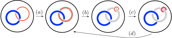
Figure 7: Using the drilling stick, identical surgery, and rational equivalent surgery, one can derive the $ST_{\alpha}$-move coming from physical analysis. This move is between the first graph and the third graph in this figure.

The rational equivalent surgery changes linking numbers, which is basically a Dehn-twist of meridian, namely $\text{Im}(\alpha)=\alpha^{\prime}+t\beta^{\prime}$, as we have shown in (72), and this twist turns $L(1,0)$ into $L(1,t)$. If we perform $t$ numbers of twists on the circle $L_{i}$, then it also twists its linked circles $L_{j}$ to $\tilde{L}_{j}$. Their linking numbers become

$$\tilde{k}_{i}=\frac{1}{t+\frac{1}{k_{i}}}\,,\leavevmode\nobreak\ \leavevmode\nobreak\ \tilde{k}_{j}=k_{j}+t(L_{i}\cdot L_{j})^{2}\,,\leavevmode\nobreak\ \leavevmode\nobreak\ \tilde{k}_{ij}=k_{ij}\,,$$ (87)

$$\tilde{L}_{i}\cdot\tilde{L}_{j}=\tilde{k}_{ij}\,,\leavevmode\nobreak\ L_{i}\cdot L_{j}=k_{ij}\,,\leavevmode\nobreak\ \tilde{L}_{i}\cdot\tilde{L}_{i}:=\tilde{k}_{i}\,,\leavevmode\nobreak\ \tilde{L}_{j}\cdot\tilde{L}_{j}:=\tilde{k}_{j}\,.$$ (88)

The rational equivalent surgeries put strong constraints on the framing numbers, since they should be integral numbers. This type of equivalent surgeries does not fall in the class of Kirby moves, and is called rational calculus by Rolfsen in Rolfesn:1984 .

If introducing a charge-$q$ matter on $L(k,1)$, one can get the link graphs for $ST_{\alpha}$-move:

(89)

where we have assigned effective framing numbers. The charge $q$ as the linking number does not change under the $ST$-moves (or rational calculus). Note that after the rational twist, the matter circle should not link to the previous gauge circle (blue circle). Moreover, since $k$ is the effective CS level, we should assume it has already received corrections from matters. However, for the $S^{3}_{\infty}$, since it has a $\infty$-framing number, it is insensitive to any corrections from matters. The linking numbers of circles in (89) match with that of $ST$-moves on plumbing graphs:

(90)

which is the graph in (4), and here we assigned effective CS levels. If we delete gauge nodes $\bullet_{k}$ and $\bullet_{k+q^{2}}$, the $ST$-moves reduce to the mirror duality between $1\textbf{F}\leftrightarrow U(1)_{\pm 1}+1\textbf{F}$

(91)

Correspondingly, If one deletes the blue circles in (89), a free matter would be a $L(1,0)$ with a defect on its longitude and the theory $U(1)_{\pm 1}+1\textbf{F}$ is $L(\pm 1,1)$ with a defect on the meridian. Then mirror tirality can be represented as

(92)

This mirror triality is highly non-trivial, as it means that even if the matter circle (Lagrangian defect) is present, the rational twist is still a homemorphism. Note that we should not draw the ${\color[rgb]{1,0,0}{\bigcirc}}$ along the longitude of $N(\bigcirc_{\pm 1})$ because of many reasons. One of them is that $L(\pm 1,1)$ should be viewed as a standard Lens space. Another reason is to be consistent with handle-slides below. From brane webs, a local S-duality should switch the type of defect brane from $\text{NS}5$ to $\text{D}5$.

It seems that rational equivalent surgeries lead to the same plumbing/circle graphs as handle-slides that was discussed in section 2. We know how to freely introduce a $S^{3}_{\infty}$ but not $S^{3}_{\infty}\backslash{\color[rgb]{1,0,0}{\bigcirc}}$. Fortunately, handle-slides, such as (22) may tell us how to introduce it. We still need to use $S^{3}_{\pm 1}\backslash{\color[rgb]{1,0,0}{\bigcirc}}$ and then apply the handle-slide operation by recombining gauge circles. Finally, we apply rational twist to get $S^{3}_{\infty}\backslash{\color[rgb]{1,0,0}{\bigcirc}}$. We use the graph below to illustrate this process:

(93)

where the twist is the reverse of process $(b)$ in Figure 7. For bifundamental matter, the straightforward application of drilling and rational surgery could indeed derive (22).

For the linked matter circles, $ST$-moves could separate them. For instance,

(94)

Note that if a gauge circle $\bullet_{k}$ links to a $S^{3}_{\infty}$, we cannot directly apply $\alpha$-Kirby moves to integrate out $\bullet_{k}$, as $\infty$ could eat any number.

Trefoils. One can consider complicated matter circle linking to a trefoil. As a typical knot in textbook e.g. Prasolovbook ; Rolfesn:1984 ; Rolfsenbook , the trefoil can be unknoted by $\alpha$-Kirby moves into the link $\bullet_{k}-\bullet_{\pm 1}$ with linking number $\pm 2$. One can also insert a complicated matter circle ${\color[rgb]{1,0,0}{\bigcirc}}_{\infty}$ on this $\bullet_{\pm 1}$ as follows:

(95)

which engineers a theory $U(1)_{k^{\prime}}$ with a charge-2 matter. Note that matter circles could have many other ways to tangle with trefoils depending on how to insert matter circles, which are much more complicated than examples in this note.

5 Open problems

The surgery constructions of 3d theories depend mainly on the topology of three-manifolds, which translate dualities in terms of geometric transformations. There are many related open problems:

• One problem is to engineer superpotentials, and find the corresponding geometric objects in three-manifolds. We hope the gauged SQED-XYZ duality Cheng:2023ocj , which encodes the simple cubic superpotential $\mathcal{W}=XYZ$, could be interpreted as some combinatorial relations of matter circles. The surgery construction in this note should be extended to non-abelian theories, which is straightforward for Lens spaces. For non-abelian theories, $W^{\pm}$-bosons should be carefully realized. Monopole operators in Benvenuti:2016wet should also be considered to complete the construction.

• The matter circles we have considered in this note are unknotted. Generically, matter circles could be knots suggested by Ooguri-Vafa construction, which intersect the three-manifolds along knots, namely $L_{\color[rgb]{1,0,0}K}\cap M_{3}={\color[rgb]{1,0,0}K}$. Then we should call ${\color[rgb]{1,0,0}K}$ the matter knot. If it is possible to transform the matter knot ${\color[rgb]{1,0,0}K}$ into links of simple matter circles ${\color[rgb]{1,0,0}{\bigcirc}}$, the nature of knots could be significantly uncovered, and the encoded gauge theories can be read off. The RT invariants of $M_{3}\backslash{\color[rgb]{1,0,0}K}$ could be useful to address many physical aspects of the underling gauge theories. Some results from mathematical works such as Chen:2015wfa could be translated into physics.

• We expect the further development of surgery construction could provide a systematic derivation of knots-quivers correspondence Kucharski:2017poe ; Kucharski:2017ogk . The expected correspondences between Wilson loops and matter defects may provide more details to 3d-3d correspondence.

• There are multiple ways to insert matter circles to three-manifolds, and they can be deformed and combined. We hope the modular tensor category (MTC) can be used to describe the relations and fusions of matter circles. The mapping class group of torus is also useful to analyze the images of matter circles, which is a problem that we have not managed to solve in this note.

• There are some gaps to connect surgery constructions of 3d theories with the Large-N transitions of Lens spaces Gopakumar:1998ki ; Labastida:2000yw . It seems that the fiber and base should be reversed to match them, since during the large-N transition, Lens space should correspond to the flavor symmetry and Lagrangian brane $L_{K}$ corresponds to the gauge group, which is opposite to surgery construction and thus is mysterious.

• We have not considered hyperbolic structures yet, which however are very useful in the DGG construction. Finding the role played by hyperbolic structure and metric would be an interesting direction.

• In Cecotti:2011iy ; Dimofte:2013lba , the branched covering realization of 3d theories through 4d Seiberg-Witten curves is established, which seems similar to the surgery construction in many aspects. We hope to find the relations between these constructions.

Appendix A Lens space

The Lens spaces are the orbifold of three-sphere $L(k,1)=S^{3}/\mathbb{Z}_{k}$. If complex coordinates are given, the definition is $|z_{1}|^{2}+|z_{2}|^{2}=r^{2}$ with the $\mathbb{Z}_{k}$ action $(z_{1},z_{2})\mapsto(e^{\frac{2\pi\,i}{k}}z_{1},e^{\frac{2\pi\,i}{k}}z_{2})$. The homology is $H_{1}(L(k,1))=\mathbb{Z}_{k}$ and $L(2,1)=S^{3}/\mathbb{Z}_{2}=\mathbb{RP}^{3}$. For generic Lens space, there are equivalences that $L(p,q)=L(p,q+np)=L(-p,q)$, so $L(k,1)=L(\frac{k}{nk+1},1)$. Lens spaces are special Lagrangian submanifolds insider the Calabi-Yau three-folds $T^{*}L(k,1)$. As special examples of Seifert manifolds, Lens spaces are circle bundles over a two-sphere: $\mathcal{O}(-k)\hookrightarrow L(k,1)\xrightarrow{\pi}{\mathbb{P}^{1}}$.

The plumbing manifolds are given by gluing a couple of Lens spaces by Dehn surgeries, which are performed by extending circles of framing number $k$ to a solid torus. Then the Lens space is denoted by this circle. The plumbing graphs are made to denote the links for surgeries. We use the example below to illustrate:

$$\begin{split}\includegraphics[width=252.94499pt]{figgeo/plumbgraphex.pdf}\end{split}$$ (96)

where each black node denotes a lens space $L(k,1)$, and the linking numbers denote the lines. Because of orientations, there could be different signs. By extending this examples, complicated plumbing graphs containing nodes and lines are links that could lead to generic three-manifolds given by Dehn surgeries along these links.

The self-linking number is known to be the framing number between the circle $L$ and its slightly deformed circle $L^{\prime}$. After deformation, there two circles have linking number $L_{i}\cdot L_{i}:=L_{i}\cdot L^{\prime}_{i}=k_{i}$. The linking number between two circles are usually defined as $L_{i}\cdot L_{j}=k_{ij}:=\frac{1}{2}\times\text{corssing number}$. We only focus on integral surgeries, as the parity anomaly requires framing numbers to be integers Aharony:1997aa .

Others. The geometry of Lagrangian defect is ${\color[rgb]{1,0,0}S^{1}}\times\mathbb{R}^{2}$ where $\mathbb{R}^{2}\subset\mathbb{R}^{3}$ and $\mathbb{R}^{3}$ is the fiber of $T^{*}M_{3}$. The intersection is the matter circle ${\color[rgb]{1,0,0}S^{1}}=({\color[rgb]{1,0,0}S^{1}}\times\mathbb{R}^{2})\cap M_{3}$. The topology of the defect can be written as ${\color[rgb]{1,0,0}S^{1}}\times\mathbb{R}^{2}=T^{2}\times\mathbb{R}_{+}$ where the $T^{2}$ degenerates to ${\color[rgb]{1,0,0}S^{1}}$ at the origin of $\mathbb{R}^{2}$. This is one half of the geometry $S^{1}\times S^{2}$ and can be represented as a half-infinite line using tori geometry.

References

- (1) S. Cheng and P. Sułkowski, 3d = 2 theories and plumbing graphs: adding matter, gauging, and new dualities, JHEP 08 (2023) 136, [arXiv:2302.13371].
- (2) K. A. Intriligator and N. Seiberg, Mirror symmetry in three-dimensional gauge theories, Phys. Lett. B387 (1996) 513–519, [hep-th/9607207].
- (3) O. Aharony, A. Hanany, K. Intriligator, N. Seiberg, and M. J. Strassler, Aspects of N=2 Supersymmetric Gauge Theories in Three Dimensions, Nucl.Phys.B 499 (1997) 67–99, [hep-th/9703110].
- (4) A. Hanany and E. Witten, Type IIB superstrings, BPS monopoles, and three-dimensional gauge dynamics, Nucl.Phys. B492 (1997) 152–190, [hep-th/9611230].
- (5) A. Kapustin and M. J. Strassler, On mirror symmetry in three-dimensional Abelian gauge theories, JHEP 04 (1999) 021, [hep-th/9902033].
- (6) N. Dorey and D. Tong, Mirror symmetry and toric geometry in three-dimensional gauge theories, JHEP 05 (2000) 018, [hep-th/9911094].
- (7) A. Giveon and D. Kutasov, Seiberg Duality in Chern-Simons Theory, Nucl. Phys. B 812 (2009) 1–11, [arXiv:0808.0360].
- (8) F. Benini, C. Closset, and S. Cremonesi, Comments on 3d seiberg-like dualities, JHEP 1110 (2011) 075, [arXiv:1108.5373].
- (9) K. Intriligator and N. Seiberg, Aspects of 3d N=2 Chern-Simons-Matter Theories, JHEP 07 (2013) 079, [arXiv:1305.1633].
- (10) L. F. Alday, P. Benetti Genolini, M. Bullimore, and M. van Loon, Refined 3d-3d Correspondence, JHEP 04 (2017) 170, [arXiv:1702.05045].
- (11) J. de Boer, K. Hori, Y. Oz, and Z. Yin, Branes and Mirror Symmetry in N=2 Supersymmetric Gauge Theories in Three Dimensions, Nucl.Phys.B 502 (1997) 107–124, [hep-th/9702154].
- (12) S. Benvenuti and S. Pasquetti, 3d = 2 mirror symmetry, pq-webs and monopole superpotentials, JHEP 08 (2016) 136, [arXiv:1605.02675].
- (13) S. Cheng, 3d = 2 brane webs and quiver matrices, JHEP 07 (2022) 107, [arXiv:2108.03696].
- (14) T. Dimofte, D. Gaiotto, and S. Gukov, Gauge Theories Labelled by Three-Manifolds, Commun. Math. Phys. 325 (2014) 367–419, [arXiv:1108.4389].
- (15) S. Gukov, P. Putrov, and C. Vafa, Fivebranes and 3-manifold homology, JHEP 07 (2017) 071, [arXiv:1602.05302].
- (16) S. Cecotti, C. Cordova, and C. Vafa, Braids, Walls, and Mirrors, arXiv:1110.2115.
- (17) Y. Terashima and M. Yamazaki, SL(2,R) Chern-Simons, Liouville, and Gauge Theory on Duality Walls, JHEP 08 (2011) 135, [arXiv:1103.5748].
- (18) S. Gukov, D. Pei, P. Putrov, and C. Vafa, BPS spectra and 3-manifold invariants, J. Knot Theor. Ramifications 29 (2020), no. 02 2040003, [arXiv:1701.06567].
- (19) M. C. N. Cheng, S. Chun, F. Ferrari, S. Gukov, and S. M. Harrison, 3d modularity, JHEP 10 (2019) 010, [arXiv:1809.10148].
- (20) A. Gadde, S. Gukov, and P. Putrov, Fivebranes and 4-manifolds, Prog. Math. 319 (2016) 155–245, [arXiv:1306.4320].
- (21) R. Kirby, A Calculus for Framed Links in , Inventiones mathematicae 45 (1978) 35–56.
- (22) H. Ooguri and C. Vafa, Knot invariants and topological strings, Nucl. Phys. B577 (2000) 419–438, [hep-th/9912123].
- (23) S. Cheng, Mirror symmetry and mixed Chern-Simons levels for Abelian 3D N=2 theories, Phys. Rev. D 104 (2021), no. 4 046011, [arXiv:2010.15074].
- (24) E. Witten, SL(2,Z) action on three-dimensional conformal field theories with Abelian symmetry, hep-th/0307041.
- (25) J. Eckhard, H. Kim, S. Schafer-Nameki, and B. Willett, Higher-form symmetries, bethe vacua, and the 3d-3d correspondence, JHEP 01 (2020) 101, [arXiv:1910.14086].
- (26) L. Bhardwaj, M. Bullimore, A. E. V. Ferrari, and S. Schafer-Nameki, Anomalies of Generalized Symmetries from Solitonic Defects, arXiv:2205.15330.
- (27) F. Benini, C. Closset, and S. Cremonesi, Quantum moduli space of Chern-Simons quivers, wrapped D6-branes and AdS4/CFT3, JHEP 09 (2011) 005, [arXiv:1105.2299].
- (28) M. Sacchi, O. Sela, and G. Zafrir, Compactifying 5d superconformal field theories to 3d, JHEP 09 (2021) 149, [arXiv:2105.01497].
- (29) C. Hwang, S. Pasquetti, and M. Sacchi, Rethinking mirror symmetry as a local duality on fields, Phys. Rev. D 106 (2022), no. 10 105014, [arXiv:2110.11362].
- (30) T. Kitao, K. Ohta, and N. Ohta, Three-dimensional gauge dynamics from brane configurations with (p,q)-fivebrane, Nucl.Phys. B539 (1999) 79–106, [hep-th/9808111].
- (31) T. Dimofte, S. Gukov, and L. Hollands, Vortex Counting and Lagrangian 3-manifolds, Lett. Math. Phys. 98 (2011) 225–287, [arXiv:1006.0977].
- (32) S. Gukov and D. Pei, Equivariant Verlinde formula from fivebranes and vortices, Commun. Math. Phys. 355 (2017), no. 1 1–50, [arXiv:1501.01310].
- (33) H.-J. Chung, T. Dimofte, S. Gukov, and P. Sułkowski, 3d-3d correspondence revisited, JHEP 1604 (2016) 140, [arXiv:1405.3663].
- (34) S. Cheng and P. Sułkowski, Refined open topological strings revisited, Phys. Rev. D 104 (2021), no. 10 106012, [arXiv:2104.00713].
- (35) D. Gaiotto and E. Witten, S-Duality of Boundary Conditions In N=4 Super Yang-Mills Theory, Adv. Theor. Math. Phys. 13 (2009), no. 3 721–896, [arXiv:0807.3720].
- (36) D. Tong, Gauge Theory. http://www.damtp.cam.ac.uk/user/tong/gaugetheory.html, 2018.
- (37) D. Rolfsen, Rational surgery calculus:extension of Kirby’s theorem, Pacific Journal of Mathematics 110 (1984), no. 2 377–386.
- (38) T. Dimofte, D. Gaiotto, and R. van der Veen, RG Domain Walls and Hybrid Triangulations, Adv. Theor. Math. Phys. 19 (2015) 137–276, [arXiv:1304.6721].
- (39) D. Rolfsen, Knots and links, vol. 346. American Mathematical Society, 1976.
- (40) D. Gang, N. Kim, M. Romo, and M. Yamazaki, Aspects of defects in 3d-3d correspondence, JHEP 10 (2016) 062, [arXiv:1510.05011].
- (41) E. Witten, Quantum field theory and the Jones polynomial, Commun. Math. Phys. 121 (1989), no. 351-399.
- (42) V. Prasolov and A. Sossinsky, Knots, Links, Braids and 3-Manifolds, vol. 154. American Mathematical Society, 1997.
- (43) P. Kucharski, M. Reineke, M. Stosic, and P. Sułkowski, BPS states, knots and quivers, Phys. Rev. D96 (2017), no. 12 121902, [arXiv:1707.02991].
- (44) P. Kucharski, M. Reineke, M. Stosic, and P. Sułkowski, Knots-quivers correspondence, Adv. Theor. Math. Phys. 23 (2019) 1849–1902, [arXiv:1707.04017].
- (45) Q. Chen and T. Yang, Volume conjectures for the Reshetikhin–Turaev and the Turaev–Viro invariants, Quantum Topol. 9 (2018), no. 3 419–460, [arXiv:1503.02547].
- (46) R. Gopakumar and C. Vafa, On the gauge theory / geometry correspondence, Adv. Theor. Math. Phys. 3 (1999) 1415–1443, [hep-th/9811131].
- (47) J. M. F. Labastida, M. Marino, and C. Vafa, Knots, links and branes at large N, JHEP 11 (2000) 007, [hep-th/0010102].