VQE-inspired optimization for spin chains work extraction

Abstract

The energy extraction from quantum sources is a key task to develop new quantum devices such as Quantum Batteries (QB). In this context, one of the main figures of merit is the ergotropy, which measures the maximal amount of energy (as work) that can be extracted from the quantum source by means of unitary operations. One of the main issues to fully extract energy from the quantum source is the assumption that any unitary operation can be done on the system. This assumption, in general, fails in practice since the operations that can be done are limited and depend on the quantum hardware (experimental platform) one has available. In this work, we propose a new approach to optimize the extractable energy inspired by the Variational Quantum Eigensolver (VQE) algorithm. In this approach, we explicitly take into account a limited set of unitaries by using the Hardware Efficient Ansatz (HEA) class of parameterized quantum circuits. As a QB we use an 1D spin chain described by a family of paradigmatic first neighbour hamiltonians such as the XXX, XXZ, XYZ, XX, XY and Transverse Ising models. By building our parameterized quantum circuits assuming that different types of connectivity may be available depending on the quantum hardware, we numerically compare the efficiency of work extraction for each model. Our results show that the best efficiency is generally obtained with quantum circuits that have connectivity between first neighbour spins.

I Introduction

The development of new techniques and protocols to efficiently store, transfer and use energy on demand is arguably one of the most important goals of human kind currently [1, 2]. In the last decades, the emergent field of Quantum Information and Quantum Thermodynamics allowed us to explore how intrinsic quantum phenomena can impact in the energetics of quantum systems [3, 4, 5, 6, 7, 8]. In this context, Alick and Fannes proposed [9] a device termed Quantum Battery (QB), in which they sought to explore how non-classical features such as entanglement and coherence could be used as resources to efficiently extract work from an ensemble of quantum systems. After this seminal work, QBs have been extensively explored with the perspective that these resources could be used to achieve better performance than its classical counterparts [10, 11, 12, 13, 14]. For instance, a very promising property that arose from QBs composed by multiple quantum systems is the possibility to have a superextensive power charging scaling, which means that charging power grows faster than the number of systems in the QB [15].

When dealing with QBs, one of the central figures of merit is the ergotropy [16, 17, 9, 18]. The ergotropy quantifies the maximum work that can be extracted by means of unitary operations, i.e., without changing the QB’s entropy [18]. Naturally, the ergotropy depends on the quantum state of the QB (or quantum source) and on its hamiltonian. In the last years, much effort has been made to find optimal processes to charge and discharge the QB in a variety of theoretical models [19, 20, 21, 22, 23, 24, 25, 26, 27, 28]. This includes, for example, proposes of many-body QBs in which its hamiltonian has interactions between subsystems and, consequently, could have entangled eingenspectrum. Models of this type are known as spin chain QBs. The first spin chain QB model was proposed by Le et al. [29], where they study the role of anisotropy in the energetics of the Heisenberg and Ising spin chain models. Further works showed how disorder in the interactions and the dimensionality of the spin chain can enhance the performance of the QB [30, 31]. The optimal charging of dissipative spin chain batteries has also been explored in Ref. [23], where feedback control techniques are used. Another interesting result regarding spin chain models for many-body QBs is that working near phase transitions points can enhance the extractable energy and the thermodynamic efficiency [32]. Despite of all theoretical results, there are still just a few experimental works dealing with QBs in general [15, 33, 34, 35, 36], and even for proof of principles experiments there are still challenges to overcome. One of the difficulties is that, in practice, optimize the extractable work is a hard task because the unitary transformations that can be done are limited and depend on the experimental platform. Strategies to optimize the extractable work in realistic scenarios are open problems. A very recent review on the advances and the state of art in QBs can be found in Ref. [37].

At the same time, the grow in complexity of quantum computational tasks to address realistic problems in Noisy Intermediate Scale Quantum (NISQ) devices demanded the development of novel optimization protocols [38]. We can mention, among others, portfolio optimization [39, 40, 41, 42], quantum machine learning [43, 44, 45, 46, 47, 48] and the simulation of molecules, materials and other many-body systems [49, 50, 51]. A very exciting way to deal with such complex problems is using Variational Quantum Algorithms (VQA), which have been proved to be a powerful tool in a multitude of different contexts [52]. In particular, the VQA named Variational Quantum Eigensolver (VQE) [53, 54] is specifically designed to minimize the energy of many-body systems in order to find the ground state of hamiltonians. Inspired by these remarking results, the goal of this work is to propose a VQE-inspired optimization to address the optimization of the work extraction from spin chain QBs. To do this, we choose a broad family of spin chain hamiltonians as a QB. Moreover, consider a realistic limited set of quantum operations to perform the work extraction and also that we may have different connectivity depending on the quantum hardware one has available. With this, we expect that our protocol can be applied to any experimental platform that is currently available. It is worthwhile to mention that some recent works used machine learning techniques to optimize the charging and discharging processes of quantum batteries [55, 56, 25]. In particular, in Ref. [25] it is proposed a new scheme called Variational Quantum Ergotropy (VQErgo) to estimate the ergotropy in quantum batteries.

This paper is organized as follows. We start by introducing the main tools of our work in Sec. II. In Sec. II.1, we briefly review the concept of work extraction and ergotropy. In Sec. II.2 we introduce the spin chain hamiltonians describing our QB. In Sec. II.3 we describe the VQE-inspired optimization for work extraction. In Sec. III we show our results. First, we use a specific example with only two qubits and then we explore the dependence of the work extraction with the number of qubits and the anisotropies of the hamiltonian. Finally, in Sec. IV, we conclude our work and discuss possible next steps.

II Preliminaries and Methods

II.1 Work extraction and ergotropy

Given a closed quantum system described by the internal hamiltonian $H$, the amount of extractable work by means of reversible coherent operations is given by [9]

$$W(\rho,H)=E_{\rho}-{\rm Tr}\{HU\rho U^{\dagger}\},$$ (1)

where $U$ is a unitary operator and $E_{\rho}={\rm Tr}\{H\rho\}$ is the mean energy of the arbitrary state $\rho$. We assume the hamiltonian with non-degenerate eigenvalues. In this scenario, the maximal work that can be extracted from the system is called ergotropy [16, 17, 9, 18] and it is obtained by minimizing the second term of Eq. (1) over all possible unitary operations

$$\mathcal{E}\equiv W_{\rm max}(\rho,H) =E_{\rho}-\min_{U}{\rm Tr}\{HU\rho U^{\dagger}\}$$

$$=E_{\rho}-{\rm Tr}\{H\pi_{\rho}\},$$ (2)

where $\pi_{\rho}$ is called the passive state associated to $\rho$. By definition [16], no work can be extracted from a passive state by means of unitary operations. For the case in which $\rho$ is a pure state, it is clear that the passive state is the ground state of the hamiltonian $H$. However, for general mixed states, the passive state depends both on $H$ and the entropy of the state $\rho$. We note from Eq. (2) that for reach the ergotropy it is assumed that any unitary operation can be performed on the system. This assumption, however, is not usually true in realistic scenarios where one has a limited control over the systems. For this reason, to find protocols in order to optimize the work that can be extracted (or injected) from the system for different platforms is an interesting and current topic of research [19, 20, 21, 22, 23, 24, 25, 26, 27].

II.2 The models

In this work, we explore the amount of work that can be extracted from $N$ coupled spin-1/2 systems. To attain this task, we consider that the internal energy of the system is described by the following family of hamiltonians ($\hbar=1$):

$$H=-h\sum_{j=1}^{N}\sigma_{z}^{(j)}-J\sum_{j=1}^{N-1}[(1+\gamma)\sigma_{x}^{(j)}\sigma_{x}^{(j+1)}+(1-\gamma)\sigma_{y}^{(j)}\sigma_{y}^{(j+1)}+\Delta\sigma_{z}^{(j)}\sigma_{z}^{(j+1)}],$$ (3)

where $\sigma_{x}^{(k)}$, $\sigma_{y}^{(k)}$ and $\sigma_{z}^{(k)}$ are the usual Pauli matrices for the $k$-th spin-1/2 system in the basis $\{\ket{\uparrow_{k}},\ket{\downarrow_{k}}\}$. For the sake of simplicity, from now on we are going to use the term qubits when referring to the spin-1/2 systems. The parameter $J$ is the coupling between the qubits while $\gamma$ and $\Delta$ are constants that introduce anisotropies in the chain. The $h$ parameter is an external field which breaks the degeneracy of the energy levels of the hamiltonian. By selecting specific parameters $\gamma$ and $\Delta$, the family of hamiltonians (3) can be divided in the paradigmatic models described in Table 1.

Parameters	Models
$\Delta=1$, $\gamma=0$	XXX
$\Delta\neq 0$, $\gamma=0$	XXZ
$\Delta\neq 0$, $-1<\gamma<1$	XYZ
$\Delta=0$, $\gamma=0$	XX
$\Delta=0$, $-1<\gamma<1$	XY
$\Delta=0$, $\gamma=\pm 1$	Transverse Field Ising (TFI)

Table 1: Hamiltonian models.

II.3 VQE-inspired optimization

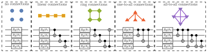
Figure 1: (colour online) Types of ansätze we are using in this work. The graphs represent the connectivity we are considering in each ansatz followed by the parameterized quantum circuit. Those are examples for 4 qubits and can be directly generalized for $N$ qubits.

The VQE optimization consists in two main ingredients. First, we need a parameterized circuit (ansatz) which imprints a set of parameters $\boldsymbol{\theta}=\{\theta_{1},\theta_{2},...,\theta_{j}\}$ on the input state $\rho$. In general, the ansatz is a unitary operation $U(\boldsymbol{\theta})$, that can be expressed as a product of successive $L$ unitaries [52]

$$U(\boldsymbol{\theta})=\mathcal{U}_{1}(\boldsymbol{\theta}_{1})\phantom{.}\mathcal{U}_{2}(\boldsymbol{\theta}_{2})\dots\mathcal{U}_{L}(\boldsymbol{\theta}_{L}),$$ (4)

with

$$\mathcal{U}_{\ell}(\boldsymbol{\theta}_{\ell})=\prod_{m}e^{-i\theta_{m}\mathcal{O}_{m}}\Lambda_{m}.$$ (5)

In Eq. (5), $\mathcal{O}_{m}$ is a hermitean operator and $\Lambda_{m}$ is an unparameterized unitary. In particular, we are going to use some ansätze belonging to the class of the Hardware Efficient Ansatz (HEA) [57, 52, 54]. The main characteristic of the HEA ansatz is that it can be tailored for a specific quantum device (experimental platform) in which one wants to run the protocol. In this class of ansätze, the unitaries are taken from a limited set of gates which are determined from the native connectivity for the chosen device. Moreover, in Ref. [58] it is shown that HEA can be used to tailor more expressive parameterized operations using less entangling gates, which provides a better efficiency to the problem of finding ground states of some small molecules. Adding to that, in Ref. [59] ts is shown that HEA can be used to find ground states of small spin chain systems with reasonable accuracy. As discussed in Ref. [54], using HEA in a VQE optimization process is a very convenient tool to proof of principles when dealing with a small number of quantum systems. These latter results motivate even more using HEA in our work, since we focus on small controllable chains (up to 8 qubits). The ansätze we are considering in this work are shown in Fig. 1, where $R_{y}(\theta_{k})=e^{-i\theta_{k}\sigma_{y}^{(k)}}$ is a local rotation of the $k$-th qubit around the $y$ axis in Bloch sphere. Each depicted ansatz corresponds to a specific connectivity that may be available for a chosen quantum hardware.

The second ingredient is the definition of a cost (or loss) function which encodes our problem solution. As we are interested in the extractable work from the quantum source defined by the hamiltonian in Eq. (3) and an input state $\rho$, we can naturally define the cost function as

$$W(\boldsymbol{\theta})=E_{\rho}-{\rm Tr}\{HU(\boldsymbol{\theta})\rho U^{\dagger}(\boldsymbol{\theta})\},$$ (6)

where $W(\boldsymbol{\theta})$ is the extractable work in Eq. (1) parameterized by the ansatz $U(\boldsymbol{\theta})$. Our task now is to optimize $W(\boldsymbol{\theta})$ for a given ansatz $U(\boldsymbol{\theta})$. The optimization is carried out using the following steps. We start with a random set of parameters $\boldsymbol{\theta}$ and register the value of $W(\boldsymbol{\theta})$. Then, we apply the gradient descent method, which consists in updating the set of parameters $\boldsymbol{\theta}$ using the iterative process

$$\theta_{j+1}\rightarrow\theta_{j}+k\frac{\partial W(\boldsymbol{\theta})}{\partial\theta_{j}},$$ (7)

where $k$ is the step size took towards the gradient. The iterative process in Eq. (7) is repeated until the cost function converges. Then, we obtain a set of parameters leading to $W(\boldsymbol{\theta}_{\rm opt})\equiv\mathcal{W}$, where $\mathcal{W}$ is the optimal amount of work that we can extract from $\rho$ using a given ansatz described by a parameterized circuit.

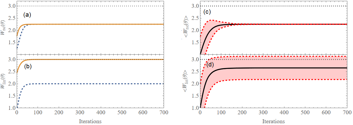
Figure 2: The plots (a) and (b) show the convergence of the cost functions given by Eqs. (14) and (15) for two different sets of initial random parameters $\{\theta_{1},\theta_{2}\}$. The plots (c) and (d) show the convergence of Eqs.(14) and (15) on average after repeating the optimization process 2000 times with initial parameters chosen randomly in the interval $[0,\pi]$. The red dashed lines depict the standard deviation from the average.

III Results

In what follows, we are going to show our results for different number of qubits in the chain described by the family of hamiltonians in Eq. (3). We are going to fix, unless otherwise stated, the input state as

$$\rho=\bigotimes_{j=1}^{N}\ket{\uparrow_{j}}\bra{\uparrow_{j}}.$$ (8)

This state is a fair assumption to illustrate our results since it can be prepared in the most of experimental platforms by means of projective measurements. We also fix the couplings $J=-1.0$ a.u. and $h=0.5$ a.u., where a.u. holds for arbitrary units. All of the following simulations were done using the software Mathematica${}^{\text{\textregistered}}$ with help of the Melt library [60].

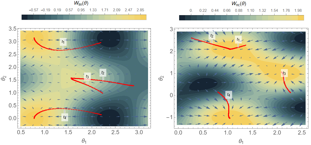
Figure 3: Plots of the cost functions landscapes. The red dots track the optimization trajectory $t_{i}$ of the parameters $\theta_{1}$ and $\theta_{2}$. For each $t_{i}$ we use a different set of random initial parameters.

III.1 Work extraction from 2 interacting qubits

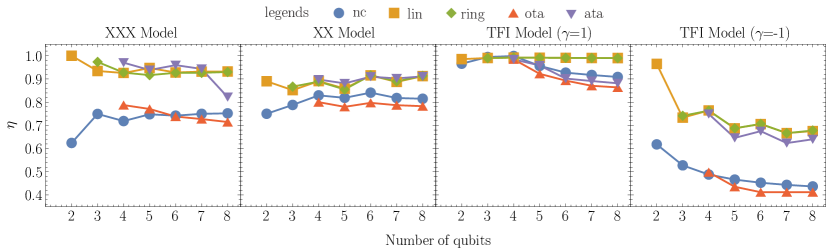
Figure 4: (colour online) Efficiency $\eta$ as in Eq. (16) as a function of $N$ for the XXX, XX and TFI models. Each pattern corresponds to a different ansatz as depicted in Fig. 1. The plot legends on the top means: no connections (nc), linear connections (lin), ring connections (ring), one-to-all connections (ota) and all-to-all connections (ata).

We start by showing our results for only two qubits ($N=2$). This case is illustrative because there are only two parameters to optimize $\{\theta_{1},\theta_{2}\}$. Then, the cost function can be visualized as a 3D function (cost function landscape), from which we can grasp some of the main features of the VQE-optimization process for work extraction. In this spirit, we choose the XX model as an example

$$H=-\frac{1}{2}\left(\sigma_{z}^{(1)}+\sigma_{z}^{(2)}\right)+\left(\sigma_{x}^{(1)}\sigma_{x}^{(2)}+\sigma_{y}^{(1)}\sigma_{y}^{(2)}\right).$$ (9)

This hamiltonian can be diagonalized, from which we can find its eigenstates

$$\ket{E_{0}}=\frac{1}{\sqrt{2}}\left(\ket{\downarrow\uparrow}-\ket{\uparrow\downarrow}\right),$$ (10)

$$\ket{E_{1}}=\ket{\downarrow\downarrow},$$ (11)

$$\ket{E_{2}}=\ket{\uparrow\uparrow},$$ (12)

$$\ket{E_{3}}=\frac{1}{\sqrt{2}}\left(\ket{\downarrow\uparrow}+\ket{\uparrow\downarrow}\right),$$ (13)

with associated energies $\{E_{0},E_{1},E_{2},E_{3}\}=\{-2,-1,1,2\}$ a.u.. As we can see, this model has a hamiltonian spectrum with entangled eigenstates. In particular, the ground state is the singlet state, Eq. (10). For two qubits, there are only two ansätze available for our protocol: linear connection between the qubits and no connections (local rotations only). For both cases, the cost function (6) can be straightforwardly computed and their analytical expressions are given by

$$W_{\rm nc}(\boldsymbol{\theta})=E_{\rho}-\cos^{2}(\theta_{1})\cos^{2}(\theta_{2})+\sin^{2}(\theta_{1})\sin^{2}(\theta_{2})-4\cos(\theta_{1})\cos(\theta_{2})\sin(\theta_{1})\sin(\theta_{2}),$$ (14)

$$W_{\rm lin}(\boldsymbol{\theta})=E_{\rho}-\left[4\cos(\theta_{1})\sin(\theta_{1})\cos(2\theta_{2})+\cos^{2}(\theta_{1})\sin^{2}(\theta_{2})-\sin^{2}(\theta_{1})\cos^{2}(\theta_{2})\right],$$ (15)

where the subscripts are for the no connections case (nc) and for the linear connection (lin) (see Fig. 1). The input state is $\rho=\outerproduct{E_{2}}{E_{2}}$ which has a mean energy of $E_{\rho}=1.0$ a.u. In this case, the passive state is $\pi_{\rho}=\outerproduct{E_{0}}{E_{0}}$, then the ergotropy [see Eq. (2)] is readily given by $\mathcal{E}=3.0$ a.u..

Firstly, let us discuss about the convergence for the different cost functions given by Eqs. (14) and (15) when running the optimization process. In Fig. 2 we show the plots for Eqs. (14) and (15) as a function of the iteration steps. We start by looking at the performance of the ansatz with no connections between the qubits. In Fig. 2(a) it is shown two examples of convergence for $W_{\rm nc}(\boldsymbol{\theta})$, each one has been initialized with a different set of initial parameters $\{\theta_{1},\theta_{2}\}$. The initial parameters were randomly selected in the interval $[0,\pi]$. It is clear that both examples converge for the same value $\mathcal{W}_{\rm nc}\approx 2.3$ a.u., which is far from the ergotropy value of $3.0$ a.u. (shown as black dotted line). On the other hand, in Fig. 2(b) we see that for different initial parameters, the cost function $W_{\rm lin}(\boldsymbol{\theta})$ does not always converge to the same value. While the trajectory described by the yellow solid line reaches the ergotropy, the blue dashed line reaches a value of $\mathcal{W}_{\rm lin}\approx 2.0$ a.u., which is less than the obtained with the no connection ansatz. Taking this into account, it is reasonable to look at the convergence of the cost functions on average. To achieve this, we repeat the optimization process $M$ times in order to obtain the average optimal extractable work $\langle\mathcal{W}\rangle$. In Figs. 2(c) and 2(d) we show the convergence of the cost functions averaged over $M=2000$ realizations of the optimization process. We can see that it is possible to extract more work on average using entangling operations, i.e, $\langle\mathcal{W}\rangle_{\rm lin}>\langle\mathcal{W}\rangle_{\rm nc}$. This is somehow expected, since the passive state is an entangled state and the input state [see Eq.(8)] is separable. The same plots show the standard deviation (red dashed line) as a function of each iteration step. It is interesting to remark that, although we can extract more work on average using the linear ansatz, its dispersion is larger than the ansatz with no-connections, which does not have any dispersion after the convergence.

To deepen our understanding about the average behaviour of the cost functions, in Fig. 3 we show the cost function landscape for both ansätze. The vectors within the contour plots represent the gradient of the cost function. The red lines track some trajectories of the parameters in the parameter space during the optimization process. Each trajectory is obtained from a different set of initial random parameters. For the ansatz with no connections we see that even though we have different trajectories, they always converge to the global maxima of the cost function. This is not the case for the linear connection ansatz. While the trajectories $t_{1}$ and $t_{4}$ converge to the maximum value of the cost function, the trajectories $t_{2}$ and $t_{3}$ get stuck in a region of the parameter space where the gradient is infinitely small (the norm of the gradient vector is represented by the arrow size). In this case, this region is due to the occurrence of local maxima in the cost function. However, as the total dimension increases, it is known that the HEA can lead to regions with highly dense local maxima and Barren Plateaus [61, 62, 63, 64, 65, 66, 54], which are large regions in the cost function landscape of parameters where the gradient vanishes.

III.2 Work extraction efficiency from $N$ interacting qubits

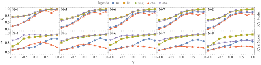
Figure 5: (colour online) Efficiency $\eta$ as in Eq. (16) as a function of the anisotropy parameter $\gamma$ for the XY (top panel) and XYZ (bottom panel) models with different number of qubits. The anisotropy parameter $\gamma$ is varied from $-1.0$ a.u. to $1.0$ a.u. in steps of $0.25$ a.u. For the XYZ model we fixed $\Delta=1.0$ a.u. for all plots. Each pattern corresponds to a different ansatz as depicted in Fig. 1. The plot legends on the top means: no connections (nc), linear connections (lin), ring connections (ring), one-to-all connections (ota) and all-to-all connections (ata).

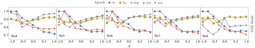
Figure 6: (colour online) Efficiency $\eta$ as in Eq.(16) as a function of the parameter $\Delta$ for the XXZ model. The parameter $\Delta$ is varied from $-1.0$ a.u. to $1.0$ a.u. in steps of $0.25$ a.u. Each pattern corresponds to a different ansatz as depicted in Fig. 1. The plot legends on the top means: no connections (nc), linear connections (lin), ring connections (ring), one-to-all connections (ota) and all-to-all connections (ata).

We shall now present our results for chains up to 8 qubits. It is convenient to define the efficiency of the work extraction protocol as

$$\eta=\frac{\langle\mathcal{W}\rangle}{\mathcal{E}},$$ (16)

which is a dimensionless quantity varying from 0 to 1. This efficiency quantifies how close we can get to the ergotropy using a given ansatz. Firstly, we analyse the performance of our protocol for the paradigmatic XXX, XX and TFI models. In Fig. 4, we show the behaviour of $\eta$ with the number of qubits for each model using the ansätze described in Fig. 1. An interesting result is that the ansatz with no connections, i.e., no entangling operations, achieves a high efficiency (more than 0.9) for the TFI model with $\gamma=1.0$ a.u.. Specifically, for 3 and 4 qubits, an efficiency about $\eta\approx 0.99$ is achieved. Another interesting result, is that the efficiency obtained using the one-to-all connections ansatz decreases as the number of qubits in the chain increases. For more than five qubits, the efficiency of this ansatz is the worst one for all shown cases. This may be explained by the fact that the connectivity of the one-to-all ansatz is incompatible with the structure of the hamiltonian, which has couplings between first neighbours only. Then, one does not expect the ground state (which is the passive state) to have entanglement between distant qubits in the chain. This also explains why the linear, ring and all-to-all connection ansätze, which have entangling operations between first neighbours, presented the best efficiencies for all models.

Now, let us turn our attention to the TFI model with $\gamma=-1.0$ a.u. As we can see, its efficiency decays as $N$ increases for all ansätze, differently from what happens for the TFI model with $\gamma=1.0$ a.u. This suggests that the anisotropy parameter $\gamma$ plays an important role in the amount of work that can be extracted given a specific ansatz. Taking this into account, we analyse the role of the anisotropy by looking at the efficiency as a function of $\gamma$ for the models XY and XYZ, as shown in Fig. 5. For the XY model, we clearly see that the amount of work that can be extracted from the spin chain increases as the anisotropy parameter $\gamma$ varies from $-1.0$ a.u. to $1.0$ a.u. for all ansätze used. The XYZ model exhibits a similar result for almost all ansätze. For $N=8$, we see that the efficiency obtained with the all-to-all ansatz suddenly decreases when compared with its value obtained for fewer qubits.

Finally, let us discuss about how the work extraction efficiency behaves as we vary the parameter $\Delta$ for the XXZ model. In Fig. 6, it is shown the plots for the efficiency as a function of $\Delta$ for the ansätze in Fig. 1 up to eight qubits. From the plots, we can see an interesting behaviour. For $\Delta<-0.25$ a.u. the no connection ansatz is the best option, and is able to extract the ergotropy for $\Delta=\{-1.0,-0.75\}$ a.u. For $\Delta>-0.75$ a.u., the entangling ansätze (with exception of the one-to-all ansatz) become more efficient than the no connection ansatz. This suggests a change on the passive state structure, which probably changes from a separable state to an entangled one.

IV Conclusions

In this work we proposed a VQE-inspired optimization to investigate the amount of work that can be extracted from first neighbour coupled qubits. We compared the efficiency of work extraction assuming different types of connectivity. Our simulation results show that the ansätze that generate entanglement between first neighbours (i.e, linear, ring and all-to-all connections) have the best performance while the one-to-all ansatz has, in general, the worst. This can be explained by the fact that the connectivity of the one-to-all ansatz is not compatible with the structure of first neighbour hamiltonians. Our results also suggest that using only local rotations can be a good strategy depending on the connectivity available and the setup of the QB (hamiltonian and number of qubits). It is worthwhile remarking that although the all-to-all present the best results, the number of CNOTs in this ansatz scales with $N(N-1)/2$, while for the linear and ring ansätze it scales with $N-1$ and $N$ respectively. In practice, the all-to-all ansatz can be problematic depending on the number of qubits in the QB since CNOT gates are more prone to errors when compared to local operations.

A natural step for future works would be explore how long range interactions in the qubits chain (as, e.g., considered in [29]) would affect the efficiency of the VQE-inspired optimization. In these cases, it is not obvious that the we will have the same hierarchy behaviour, where the ansätze that have couplings between first neighbours have the best performances. Considering effects of disordered spins also would be interesting. One could also explore how the efficiency of work extraction would be impacted by increasing the number of layers used in the ansätze shown in Fig. 1. In Ref. [59], it is demonstrated that the efficiency in finding ground states of some spin chains can be improved by considering a number of layers at least linear in the system size when using HEA-type structures built with local rotations and CZ gates. Connected to this latter work, our protocol can naturally find applications for the problem of preparing/finding the ground state of many-body hamiltonians. At this point, however, it is worth remarking that there are limitations when using the HEA class to solve optimization tasks. Even though it is a good choice for proof of principles in small systems as we stated before, for more complex and large systems such as molecular ones, the HEA is not expected to be a good option [54]. One of the issues, is that HEA is very inefficient to span very large Hilbert spaces, requiring circuits that may have exponential depth. Due to that, the HEA is very prone to Barren Plateau problems [61, 62, 63, 64, 65, 66, 54]. Nevertheless, finding optimal HEA structures and develop optimal ansätze targeted to specific complex tasks are both ongoing topics of research.

Finally, we would like to mention that recently a Variational Algorithm to estimate the ergotropy from quantum many-body batteries was proposed in [25]. In this work the authors develop an algorithm, called Variational Quantum Ergotropy (VQErgo), to find the optimal unitary for the work extraction from the QB. In their work, the QB is modelled by the internal local hamiltonian $H=-h\sum_{j}\sigma_{z}^{(j)}$ and subjected to a drive which induces a Tranverse Ising coupling used to charge/discharge the QB. Although similar in spirit, it is a very different approach from ours. First, we have considered our QB to be encoded in a spin chain hamiltonian. Second, our ansätze were built taking into account the connectivity that may be available for different quantum platforms. Said that, we truly believe that both approaches give important contributions to the areas of quantum thermodynamics and variational quantum algorithms.

- [1] Y. Dubi and M. Di Ventra. Colloquium: Heat flow and thermoelectricity in atomic and molecular junctions. Rev. Mod. Phys., 83, 131 (2011).
- [2] A. Auffèves. Quantum Technologies Need a Quantum Energy Initiative. PRX Quantum 3, 020101 (2022).
- [3] F. Binder et al. Thermodynamics in the Quantum Regime. Springer International Publishing, 2018.
- [4] Patrice A. Camati, Jonas F. G. Santos, and Roberto M. Serra. Coherence effects in the performance of the quantum Otto heat engine. Phys. Rev. A 99, 062103 (2019).
- [5] K. Micadei et al. Reversing the direction of heat flow using quantum correlations. Nat. Comm. 10, 2456 (2019).
- [6] I. Medina, S. V. Moreira, and F. L. Semião. Quantum versus classical transport of energy in coupled two-level systems. Phys. Rev. A 103, 052216 (2021).
- [7] I. Henao and R. M. Serra. Role of quantum coherence in the thermodynamics of energy transfer. Phys. Rev. E 97, 062105 (2018).
- [8] A. A. Cifuentes and F. L. Semião. Energy transport in the presence of entanglement. Phys. Rev. A 95, 062302 (2017).
- [9] R. Alicki and M. Fannes. Entanglement boost for extractable work from ensembles of quantum batteries. Phys. Rev. E 87, 042123 (2013).
- [10] G. Francica, F. C. Binder, G. Guarnieri, M. T. Mitchison, J. Goold, and F. Plastina. Quantum Coherence and Ergotropy. Phys. Rev. Lett 125, 180603 (2020).
- [11] S. Tirone, R. Salvia, S. Chessa, and V. Giovannetti. Quantum work extraction efficiency for noisy quantum batteries: the role of coherence, arXiv:2305.16803 (2023).
- [12] F. C. Binder, S. Vinjanampathy, K. Modi, and J. Goold. Quantacell: powerful charging of quantum batteries. N. J. Phys. 17, 075015 (2015).
- [13] J.-X. Liu, H.-L. Shi, Y.-H. Shi, X.-H. Wang, and W.-L Yang. Entanglement and work extraction in the central-spin quantum battery. Phys. Rev. B 104, 245418 (2021).
- [14] B. Çakmak. Ergotropy from coherences in an open quantum system. Phys. Rev. E 102, 042111 (2020).
- [15] James Q. Quach et al. Superabsorption in an organic microcavity: Toward a quantum battery. Sci. Adv. 8, eabk3160 (2022).
- [16] A. E. Allahverdyan, R. Balian, and Th. M. Nieuwenhuizen. Maximal work extraction from finite quantum systems. Europhy. Lett. 67, 565 (2004).
- [17] A. Lenard. Thermodynamical proof of the Gibbs formula for elementary quantum systems. J. Stat. Phys. 19, 575 (1978).
- [18] A. Sone and S. Deffner. Quantum and classical ergotropy from relative entropies. Entropy 23, 1107 (2021).
- [19] F. Mazzoncini, V. Cavina, G. M. Andolina, P. A. Erdman, and V. Giovannetti. Optimal control methods for quantum batteries. Phys. Rev. A 107, 032218 (2023).
- [20] G. Manzano, F. Plastina, and R. Zambrini. Optimal Work Extraction and Thermodynamics of Quantum Measurements and Correlations. Phys. Rev. Lett. 121, 120602 (2018).
- [21] W. Lu, J. Chen, L.-M. Kuang, and X. Wang. Optimal state for a Tavis-Cummings quantum battery via the Bethe ansatz method. Phys. Rev. A 104, 043706 (2021).
- [22] N. Lörch, C. Bruder, N. Brunner, and P. P. Hofer. Optimal work extraction from quantum states by photo-assisted Cooper pair tunneling. Quant. Sci. and Tech. 3, 035014 (2018).
- [23] Y. Yao and X. Q. Shao. Optimal charging of open spin-chain quantum batteries via homodyne-based feedback control. Phys. Rev. E 106, 014138 (2022).
- [24] K. V. Hovhannisyan, M. Perarnau-Llobet, M. Huber, and A. Acín. Entanglement Generation is Not Necessary for Optimal Work Extraction. Phys. Rev. Lett. 111, 240401 (2013).
- [25] D. T. Hoang et al. Variational quantum algorithm for ergotropy estimation in quantum many-body batteries, arXiv:2308.03334 (2023).
- [26] D. Šafránek, D. Rosa, and F. C. Binder. Work Extraction from Unknown Quantum Sources. Phys. Rev. Lett. 130, 210401 (2023).
- [27] D. Ferraro, M. Campisi, G. M. Andolina, V. Pellegrini, and M. Polini. High-Power Collective Charging of a Solid-State Quantum Battery. Phys. Rev. Lett. 120, 117702 (2018).
- [28] J. Liu, D. Segal, and G. Hanna. Loss-Free Excitonic Quantum Battery. J. Phys. Chem. C 123, 18303 (2019).
- [29] T. P. Le, J. Levinsen, K. Modi, M. M. Parish, and F. A. Pollock. Spin-chain model of a many-body quantum battery. Phys. Rev. A 97, 022106 (2018).
- [30] S. Ghosh, T. Chanda, and A. Sen(De). Enhancement in the performance of a quantum battery by ordered and disordered interactions. Phys. Rev. A 101, Mar 032115 (2020).
- [31] S. Ghosh and A. Sen(De). Dimensional enhancements in a quantum battery with imperfections. Phys. Rev. A 105, 022628 (2022).
- [32] F. Barra, K. V. Hovhannisyan, and A. Imparato. Quantum batteries at the verge of a phase transition. N. J. Phys. 24, 015003 (2022).
- [33] I. M. de B. Wenniger et al. Experimental analysis of energy transfers between a quantum emitter and light fields, arXiv:2202.01109 (2023).
- [34] C.-K. Hu et al. Optimal charging of a superconducting quantum battery. Quant. Sci. Tech., 045018 (2022).
- [35] J. Joshi and T. S. Mahesh. Experimental investigation of a quantum battery using star-topology NMR spin systems. Phys. Rev. A 106, 042601 (2022).
- [36] R. H. Zheng, W. N., Z. B. Yang, Y. X., and S. B. Zheng. Demonstration of dynamical control of three-level open systems with a superconducting qutrit. N. J. Phys. 24, 063031 (2022).
- [37] F. Campaioli, S. Gherardini, J. Q. Quach, M. Polini, and G. M. Andolina. Colloquium: Quantum Batteries, 2308.02277 (2023).
- [38] John Preskill. Quantum computing in the NISQ era and beyond. Quantum 2, 79 (2018).
- [39] A. Canabarro, T. M. Mendonça, R. Nery, G. Moreno, A. S. Albino, G. F. de Jesus, and R. Chaves. Quantum Finance: a tutorial on quantum computing applied to the financial market. arXiv:2208.04382 (2022).
- [40] S. Brandhofer et al. Benchmarking the performance of portfolio optimization with QAOA. Quant. Info. Process. 22, 25 (2022).
- [41] R. Yalovetzky, P. Minssen, D. Herman, and M. Pistoia. Hybrid HHL with Dynamic Quantum Circuits on Real Hardware. arXiv:2110.15958 (2021).
- [42] K. Kubo, K. Miyamoto, K. Mitarai, and K. Fujii. Pricing Multi-asset Derivatives by Variational Quantum Algorithms. IEEE Transact. Quant. Eng. 4, 1 (2023).
- [43] J. Biamonte, P. Wittek, N. Pancotti, P. Rebentrost, N. Wiebe, and S. Lloyd. Quantum machine learning. Nature 549, 195 (2017).
- [44] L. Schatzki, M. Larocca, Q. T. Nguyen, F. Sauvage, and M. Cerezo. Theoretical Guarantees for Permutation-Equivariant Quantum Neural Networks, arXiv:2210.09974 (2022).
- [45] J. J. Meyer, M. Mularski, E. Gil-Fuster, A. A. Mele, F. Arzani, A. Wilms, and J. Eisert. Exploiting Symmetry in Variational Quantum Machine Learning. PRX Quantum 4, 010328 (2023).
- [46] M. Benedetti, E. Lloyd, S. Sack, and M. Fiorentini. Parameterized quantum circuits as machine learning models. Quant. Sci. Tech. 4, 043001 (2019).
- [47] M. Schuld, I. Sinayskiy, and F. Petruccione. An introduction to quantum machine learning. Contemp. Phys. 56, 172 (2015).
- [48] M. Cerezo, G. Verdon, H.-Y. Huang, L. Cincio, and P. J. Coles. Challenges and opportunities in quantum machine learning. Nat. Comput. Sci. 2, 567 (2022).
- [49] A. Delgado, J. M. Arrazola, S. Jahangiri, Z. Niu, J. Izaac, C. Roberts, and N. Killoran. Variational quantum algorithm for molecular geometry optimization. Phys. Rev. A 104, 052402 (2021).
- [50] C. K. Lee, P. Patil, S. Zhang, and C. Y. Hsieh. Neural-network variational quantum algorithm for simulating many-body dynamics. Phys. Rev. Res. 3, 023095 (2021).
- [51] I. Stetcu, A. Baroni, and J. Carlson. Variational approaches to constructing the many-body nuclear ground state for quantum computing. Phys. Rev. C 105, 064308 (2022).
- [52] M. Cerezo et al. Variational quantum algorithms. Nat. Rev. Phys. 3, 625 (2021).
- [53] A. Peruzzo, J. McClean, P. Shadbolt, M.-H. Yung, X.-Q. Zhou, P. J. Love, A. Aspuru-Guzik, and J. L. O’brien. A variational eigenvalue solver on a photonic quantum processor. Nat. Comm. 5, 1 (2014).
- [54] J. Tilly et al. The variational quantum eigensolver: a review of methods and best practices. Physics Reports 986, 1 (2022).
- [55] P. A. Erdman, G. M. Andolina, V. Giovannetti, and F. Noé. Reinforcement learning optimization of the charging of a Dicke quantum battery, arXiv:2212.12397 (2022).
- [56] C. Rodríguez, D. Rosa, and J. Olle. AI-discovery of a new charging protocol in a micromaser quantum battery, arXiv:2301.09408 (2023).
- [57] A. Kandala, A. Mezzacapo, K. Temme, M. Takita, M. Brink, J. M. Chow, and J. M. Gambetta. Hardware-efficient variational quantum eigensolver for small molecules and quantum magnets. Nature 549, 242 (2017).
- [58] A. Wu, G. Li, Y. Wang, B. Feng, Y. Ding, and Y. Xie. Towards Efficient Ansatz Architecture for Variational Quantum Algorithms, arXiv:2111.13730 (2021).
- [59] C. Bravo-Prieto, J. Lumbreras-Zarapico, L. Tagliacozzo, and J. I. Latorre. Scaling of variational quantum circuit depth for condensed matter systems. Quantum 4, 272 (2020).
- [60] https://melt1.notion.site/ - Melt libray website.
- [61] M. Cerezo, A. Sone, T. J. Volkoff, L. Cincio, and P. J. Coles. Cost function dependent barren plateaus in shallow parametrized quantum circuits. Nat. Comm. 12, 1791 (2021).
- [62] M. Cerezo, P. Czarnik, K. l. Sharma, G. Muraleedharan, P. Coles, and M. Larocca. Diagnosing barren plateaus with tools from quantum optimal control. Quantum 6, 824 (2022).
- [63] J. Liu, Z. Lin, and L. Jiang. Laziness, barren plateau, and noise in machine learning. arXiv:2206.09313 (2022).
- [64] E. C. Martín, K. Plekhanov, and M.l Lubasch. Barren plateaus in quantum tensor network optimization. Quantum 7, 974 (2023).
- [65] J. R. McClean, S. Boixo, V. N. Smelyanskiy, R. Babbush, and H. Neven. Barren plateaus in quantum neural network training landscapes. Nat. Comm. 9, 4812 (2018).
- [66] Z. Holmes, K. Sharma, M. Cerezo, and P. J. Coles. Connecting Ansatz Expressibility to Gradient Magnitudes and Barren Plateaus. PRX Quantum 3, 010313 (2022).