Hybrid quantum-classical algorithm for the transverse-field Ising model in the thermodynamic limit

Abstract

We describe a hybrid quantum-classical approach to treat quantum many-body systems in the thermodynamic limit. This is done by combining numerical linked-cluster expansions (NLCE) with the variational quantum eigensolver (VQE). Here, the VQE algorithm is used as a cluster solver within the NLCE. We test our hybrid quantum-classical algorithm (NLCE$+$VQE) for the ferromagnetic transverse-field Ising model on the one-dimensional chain and the two-dimensional square lattice. The calculation of ground-state energies on each open cluster demands a modified Hamiltonian variational ansatz for the VQE. One major finding is convergence of NLCE$+$VQE to the conventional NLCE result in the thermodynamic limit when at least $N/2$ layers are used in the VQE ansatz for each cluster with $N$ sites. Our approach demonstrates the fruitful connection of techniques known from correlated quantum many-body systems with hybrid algorithms explored on existing quantum-computing devices.

1 Introduction

Quantum computers in the noisy intermediate scale quantum (NISQ) era are essential tools for the quantum many-body systems to test the potential advantage over conventional classical methods. Therefore, it is inevitable to explore the advantages that quantum algorithms can impart to the existing problems of classical computers, which are limited by the exponential growth of Hilbert space with the increase in size of quantum systems. Indeed, all existing classical methods for solving quantum many-body lattice systems such as tensor networks  [1, 2] , quantum Monte Carlo techniques  [3], density matrix renormalization group  [4, 5], etc., have their individual limitations. As a consequence, hybrid quantum-classical algorithms such as variational quantum eigensolver (VQE)[6], quantum adiabatic optimization algorithm (QAOA)[7], CQE (contracted quantum eigensolver) [8], etc are gaining popularity in promising to solve the problem of exponential Hilbert space growth with a potential speed-up and within a range of acceptable errors.

One such hybrid algorithm is the variational quantum eigensolver (VQE), developed by Perruzo et al. [6], which uses a union of classical and quantum computation to minimize a cost function. The VQE algorithm is not only more resilient to quantum errors as compared to other quantum algorithms [9] but also requires low coherence times [10], making it one of the most promising NISQ algorithm. Additionally, VQE can be implemented on all quantum hardware. It can therefore be an efficient tool to investigate the properties of quantum many-body systems.

However, the existing NISQ devices and the use of quantum-classical algorithms like VQE are highly limited due to small number of available (noisy) qubits. Obviously, it would be desirable to overcome this limitation and to determine, at least in an approximate fashion, the properties of quantum many-body lattice problems in the thermodynamic limit exploiting available quantum computers. Interestingly, in classical computation, several approaches exist that can be used to approximate the properties of a quantum system in the thermodynamic limit. In particular, series expansion methods such as linked-cluster expansions (LCE) [11, 12] exploit a full graph decomposition to determine physical quantities in the thermodynamic limit by perturbative calculations on finite graphs. A non-perturbative extension of LCEs are numerical linked-cluster expansions (NLCE) [13, 14], which deduce energies and observables in the thermodynamic limit by replacing perturbation theory on graphs with non-perturbative tools like exact diagonalization (ED). The NLCE method has been used successfully to study properties of various materials [15, 16, 17, 18], quantum dynamics [19, 20], and thermodynamic properties of systems [21, 22]. NLCEs were also successfully applied to calculate excitation energies of quantum many-body systems using contractor renormalization group (CORE) [23] with ED and graph-based continuous-unitary transformations (gCUT) [24, 25]. Only recently the approach utilizing ED was generalized to non-parity broken models and arbitrary number of excitations using projective cluster-additive transformations (pCAT) [26]. NLCEs are known to converge when the spatial correlations in the system do not exceed the sizes of the graphs considered. However, the use of ED as solver on the graphs limits current NLCE calculations due to the exponential growth of the Hilbert space. In addition, also the number of graphs increases exponentially with the number of sites.

In this work we explore a hybridization of NLCE and the quantum-classical algorithm VQE, dubbed NLCE+VQE, in order to go beyond their respective limitations and to fuse their advantages. Hence, we integrate VQE, as a graph solver within the NLCE replacing ED. For this purpose, we use ideal statevector simulations for the VQE throughout the paper. The calculation of ground-state energies on each open cluster demands a modified Hamiltonian variational ansatz for the VQE. We benchmark NLCE+VQE for the ferromagnetic transverse-field Ising model (TFIM) on the one-dimensional chain and the two-dimensional square lattice. This is done by calculating the ground-state energy of the high-field polarized phase in a quantitative fashion in the thermodynamic limit. The TFIM is introduced in section 2. Our NLCE+VQE approach as well as details for NLCE and VQE are described in section 3. We use VQE algorithm to compute the ground-state energy of finite clusters of a lattice model and then embed them on the infinite lattice using the NLCE. In order to improve the optimization process for the NLCE$+$VQE method, we also study the ground-state energy of periodic TFIM clusters in section 3.3. These findings are used to improve the ansatz and initial guess parameters for implementing the VQE algorithm to graphs in NLCE in section 3.4. We provide NLCE+VQE results for the TFIM on the chain and the square lattice in section 4. Finally, we conclude this work in section 5.

2 Transverse-field Ising model

The transverse-field Ising model is one of the paradigmatic models of quantum many-body physics. Since it is exactly solvable in one dimension, the TFIM can act as a good system to benchmark the efficiency of quantum-classical hybrid algorithms against classical computational approaches. The Hamiltonian for the transverse-field Ising model is given by

$$H=-\,h\sum_{\nu}Z_{\nu}-J\sum_{<\nu,\,\mu>}X_{\nu}X_{\mu},$$ (1)

where $J$ is the coupling constant and $h$ is the external field applied in a transverse direction. $Z$ and $X$ are Pauli matrices. For $J\gg h$ and $J>0$ ($J<0$), the model is in a ferromagnetic (antiferromagnetic) Ising-phase when we restrict to unfrustrated lattices. The Hamiltonian given in Eq. 1 has $\mathbb{Z}_{2}$ symmetry and remains invariant under the action of flipping all the spins. The one-dimensional transverse-field Ising chain is exactly solvable by mapping the Hamiltonian to a quadratic fermionic one with the Jordan-Wigner transform and subsequently solving it with the Bogoliubov transformation [27]. The system is in a disordered phase for $J/h<1$ and in the ordered Ising phase for $J/h>1$. The quantum phase transition occurs at $J/h=1$ and has same universality class as the two-dimensional classical Ising model. In general, one can map the d-dimensional TFIM to a $d+1$-dimensional classical Ising model. For the two-dimensional square lattice, the TFIM undergoes a quantum phase transition at $J/h=0.3285$ in the 3d Ising universality class [28, 29]. While on bipartite lattices, the ferromagnetic and antiferromagnetic TFIM behave identical, on non-bipartite lattices, the behaviour of the antiferromagnetic TFIM can be very different. For example on the frustrated triangular lattice, it undergoes a phase transition in the 3dXY-universality class and on the frustrated Kagome lattice, the model is in a disordered phase for any $h>0$ [30, 31]. In this work we restrict ourselves to the non-frustrated TFIM on a chain and square-lattice geometry and calculate the ground-state energy in the disordered phase with the NLCE+VQE approach.

3 NLCE$+$VQE

3.1 Numerical linked-cluster expansions

NLCEs use calculations on finite clusters to approximate properties of a system in the thermodynamic limit. We want to use NLCEs to approximate the ground-state energy of the TFIM on a chain and the square lattice. NLCEs exploit that some quantities are additive, which we will explain for the ground-state energy in the following.

The ground-state energy per site of a Hamiltonian $H=H_{A}+H_{B}$ on two disconnected clusters $A$ and $B$, where $H_{A,B}$ only acts on the space $A,B$ and $[H_{A},H_{B}]=0$ holds, is

$$E=E_{A}+E_{B}\,.$$ (2)

$E_{A,B}$ is the ground-state energy of $H_{A,B}$. We recursively define reduced energies by

$$\bar{E}_{c}=E_{c}-\sum_{c^{\prime}\subset c}E_{c^{\prime}}\,.$$ (3)

From Eq. (2) and Eq. (3) it follows that $\bar{E}_{c}=0$ for a non-linked cluster $c$. Hence, one can perform a linked-cluster expansion for the ground-state energy per site

$$e=\sum_{c}w_{c}\bar{E}_{c}\,.$$ (4)

The sum runs over all linked clusters $c$ and the embedding factor $w_{c}$ is determined by the numbers of embeddings for this graph on the lattice. Linked-cluster expansions were first used for perturbative calculations of the ground-state energy of quantum many-body systems and later generalized to calculate excitation energies [32]. Later, the concept was applied to non-perturbative calculations of thermodynamic quantities [33] and for the calculation of ground-state properties of quantum many body systems [13], albeit the idea already had been proposed much earlier [34]. For perturbative calculations convergence is limited to the convergence radius of the perturbative expansion. The situation is less clear for NLCEs. One expects quantities to converge as long as the subspace of interest is gapped. This is given for our application of NLCEs to the ground-state energy of the TFIM.

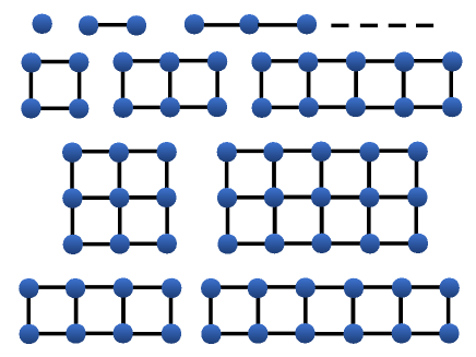
Figure 1: This figure shows the graphs used in the rectangular-graph expansion of NLCE for the TFIM on the chain (first line) and the square lattice (all graphs) up to the largest cluster size of 12 spins. It includes one-dimensional chains from one to twelve spins, ladders, and squares.

The decomposition of a lattice into finite clusters used for NLCEs is not unique. Often NLCEs are performed with all graphs of the lattice, also called full-graph expansion. In this work, we use a rectangular graph expansion for the chain and the square lattice (see Fig. 1). It coincides with the full graph expansion on the chain. In one dimension, $e=\sum_{c}w_{c}\bar{E}_{c}$ reduces to $e=E_{L}-E_{L-1}$ for all graphs up to length $L$. In two dimensions this does not hold any more because the embedding factors are not the same for all graphs and we need all reduced energies of rectangles up to a certain size to calculate the ground-state energy. The number of graphs in the rectangular-graph expansion scales polynomially with the number of sites. Fig. 1 shows the graphs used in rectangular-graph expansion up to 12 spins which includes one spin, one-dimensional chains, ladders, and square graphs. The order for this expansion is defined by the number of sites $N=L_{X}\times L_{Y}$, where $L_{X}$ and $L_{Y}$ are the widths and heights of the rectangles.

3.2 The variational quantum eigensolver algorithm

The ground-state energy of the TFIM can be computed using the Rayleigh-Ritz variational principle, which states that a parametrized wavefunction can be used to determine the upper bound to the ground-state energy

$$E_{\mathrm{gs}}\leq E(\theta)=\langle\psi(\theta)|H|\psi(\theta)\rangle.$$ (5)

This principle serves as the basis for the variational quantum eigensolver (VQE) algorithm [35]. VQE is a quantum-classical hybrid algorithm which uses a quantum computer to determine the eigenstates of a quantum many-body Hamiltonian and a classical computer to implement an optimization routine to minimize a cost function, which in our case, is the energy. A parametrized wavefunction is prepared using a unitary operation $U(\theta)|\psi\rangle$ in the first step called state preparation. In the second step, the expectation values $\langle\psi(\theta)|H_{s}|\psi(\theta)\rangle$ are determined on a quantum machine, where $H_{s}$ are the different terms in the Hamiltonian. The expectation values are further added to determine the total energy eigenvalue, which is then sent to a classical optimizer. The optimizer minimizes the energy in an iterative loop which goes over the first step, i.e., state preparation with new parameters decided by the optimization method. This is repeated until a global minimum for energy is obtained, hence, resulting in the ground-state energy for a system.

All variational quantum algorithms including VQE suffer from a common issue of difficult parameter optimization. One often finds non-convex energy landscapes in the ground-state energy of quantum many-body systems due to which the VQE algorithm is highly susceptible to errors caused by barren plateaus [36, 37] and local minima [38] during optimization. Therefore, the design of the variational ansatz is of core importance to the VQE algorithm. VQE can promise a potential advantage over conventional classical methods of computation if the quantum circuit for the ansatz can represent sufficiently accurate trial wavefunctions. The implementation of VQE on quantum hardware requires the ansatz to be not only well calibrated in expressibility and trainability but also easy to implement on quantum devices. One such ansatz for the VQE algorithm is the Hamiltonian variational ansatz (HVA) that has been used for various models such as the transverse field Ising model, XXZ model, Hubbard model and many others [36, 39, 40, 41, 42, 43, 44, 45]. An interesting feature of HVA is that its structure does not require entanglement between more than two qubits for models with only two qubit-interactions, which makes it hardware friendly. In this paper, we use the Hamiltonian variational ansatz for our VQE calculations of ground-state energies. Apart from the ansatz, the VQE algorithm most importantly solves an optimization problem, due to which the optimization strategy used becomes extremely important. VQE optimization is shown to be NP-hard [38]. A good reference state or well chosen initial guess parameters assist the VQE optimization to reach the global minima for the cost function. We investigate how to find these initial guess parameters in the subsequent sections.

3.2.1 Ansatz

The choice for $U(\theta)$ is very important for the VQE algorithm. The ansatz must have the ability to span a substantial number of states in the Hilbert space, a property known as expressibility [46]. It denotes the accuracy with which an ansatz in VQE can determine important low-energy states when the optimization reaches a global minimum. Another salient feature of the ansatz is the trainability that describes the ability of the ansatz to be optimized on a quantum device. This includes the shape of optimization landscape, optimum number of parameters and susceptibility to get stuck on barren plateaus or in local minima. The ansatz apart from being sufficiently expressible must contain an appropriate number of parameters so that it can approximate the ground-state wavefunction with acceptable accuracy. However, it should not be excessively expressible so that the wavefunction of interest becomes intractable. Also local minima are more likely to occur, if it is too expressible. Apart from these aspects, another relevant property for the ansatz is the scaling and complexity of quantum circuits with system size. It is important to have an optimum circuit depth for the ansatz that does not scale exponentially with the system size.

One good ansatz that calibrates the aforementioned features is the Hamiltonian variational ansatz (HVA) [36, 39], which is inspired by the quantum approximate optimization algorithm (QAOA) [7] and adiabatic quantum computation [47]. If the Hamiltonian is of the form $H=\sum_{s}H_{s}$, where the summation runs over all the terms in the Hamiltonian, the HVA is given by

$$U(\Theta)=\prod_{l}\big{(}\prod_{s}e^{\mathrm{i}\theta_{s,l}H_{s}}\big{)},$$ (6)

where $l$ denotes to the number of layers of HVA. There is still a freedom to choose the ordering of operators $H_{s}$ in Eq. (6). For some classes of Hamiltonians one can write $H=H_{A}+H_{B}$ with local terms in $H_{A}$ or $H_{B}$ commuting, but $[H_{A},H_{B}]\neq 0$. It is then natural to choose an ansatz, where first a layer of local (potentially differently weighted) terms of $H_{A}$ is put in the circuit, followed by a layer of $H_{B}$ and so on [7].

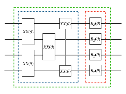
Figure 2: Quantum circuit for the Hamiltonian variational ansatz for the transverse-field Ising model with periodic boundary conditions.

The quantum circuit corresponding to the HVA is shown in Fig. 2 for the TFIM. The first block in blue color implements the Ising part of the Hamiltonian $e^{\mathrm{i}\sum_{j}\theta^{XX}_{\nu,\mu,l}X_{\nu}X_{\mu}}$ along with the boundary term. The second red block implements the transverse field term of the Hamiltonian, i.e., $e^{\mathrm{i}\sum_{\nu}\theta^{Z}_{\mu,l}Z_{j}}$. Both these blocks make up one layer, represented by a green block. These layers in the ansatz are repeated while calibrating expressibility and entanglement in the quantum circuit. It is convenient to choose as reference state

$$\ket{\mathrm{ref}}\equiv\ket{\uparrow\dots\uparrow},$$ (7)

i.e., the fully polarized state. The unitary circuit is applied to this reference state and the energy of $U(\Theta)\ket{\mathrm{ref}}=\ket{\Psi(\Theta)}$ is measured. More layers impart more parameters for optimization which may or may not help reaching the global minima depending on the optimization procedure. The energy is expected to reduce with each additional layer as $E_{l+1}(\theta)<E_{l}(\theta)$ until a convergence is reached. We investigate this convergence in subsection 3.3 and section 4, where we will see that the number of layers needed depends on the system size.

3.2.2 Optimization

The VQE algorithm is an optimization problem at heart as it heuristically constructs an approximation of the wavefunction through iterative training of parameters in the ansatz. A good optimization strategy helps to reach a well-approximated solution to the minimization procedure within an acceptable number of iterations. Therefore, starting with parameters already close to the real solution makes it easier for the optimizer to find global minima and also reduces the number of iterations required for optimization. Apart from that, restricting the parameter space for the optimization process decreases the potential of getting stuck on barren plateaus and local minima. Barren plateaus are a result of occurrence of vanishing gradients in the gradient descent method.

The optimization parameters can be constrained in the range $[0,\pi]$ since the HVA ansatz for the TFIM is periodic in $\pi$. This follows from

$$e^{\mathrm{i}(\varphi+\pi)X_{\nu}X_{\mu}} =e^{\mathrm{i}(\varphi+\pi)}e^{\mathrm{i}(\varphi+\pi)(X_{\nu}X_{\mu}-1)}$$ (8)

$$=-e^{\mathrm{i}\pi(X_{\nu}X_{\mu}-1)}e^{\mathrm{i}\varphi X_{\nu}X_{\mu}}$$

$$=-e^{\mathrm{i}\varphi X_{\nu}X_{\mu}}.$$

Similarly $e^{\mathrm{i}(\varphi+\pi)Z_{\nu}}=-e^{\mathrm{i}\varphi Z_{\nu}}$ holds. Hence a shift of $\pi$ in the parameters can only lead to a global phase of $-1$ when one applies the HVA (6) of the TFIM to a state.

For the process of optimization, we use the trust-constraint method [48] where we use the symmetric rank-one quasi-Newton method (SR1)  [49] as Hessian update strategy. In order to obtain the ground-state energy for a parameter region, we use a strategy we call adiabatic optimization, in which we take the optimized parameters corresponding to $J/h$ and plug it as the initial guess parameters for $J/h-\delta$. This ensures that the solution space for optimization remains small hence reducing the number of local minima in the landscape. In other words,

$$\theta^{i}_{J/h-\delta}=\theta^{f}_{J/h},$$ (9)

where $\theta^{i,(f)}_{J/h}$ are the initial (final) parameters. Adiabatic optimization heavily cuts down the number of iterations for each point in the physical parameter space. More importantly, adiabatic optimization helps avoid barren plateaus.

3.3 VQE for periodic clusters

The one-dimensional TFIM on periodic clusters was investigated with the HVA ansatz in Wiersama et al. [39]. Due to the presence of translational invariance, the HVA uses the same parameter for each sub-layer in Eq. (6), hence using only two parameters per layer. In [39] it was found that for a parameter range of $h\in[0.5,1.5]$ around the critical point $N/2$ layers are sufficient to express the true ground state of the model. Even the limiting cases are not easy to deal with. While the ground state in the limit $J=0$ can always be expressed by setting all parameters to zero, the other limit, $h=0$, requires a finite number of layers. In [50] it was proved that $N/2$ layers are necessary and sufficient to express the even parity ground state

$$\Psi_{\mathrm{gs},\,h=0}=(\ket{\leftarrow\dots\leftarrow}+\ket{\rightarrow\dots\rightarrow})/\sqrt{2}.$$ (10)

So the same number of layers as needed for the exact solution is also needed to express $\Psi_{\mathrm{gs},\,h=0}$. For odd periodic chains we found that setting all parameters to $\pi/4$ yields $\Psi_{\mathrm{gs},\,h=0}$. For even number of spins, the parameters change with the number of spins. For the calculations of the periodic TFIM with VQE we used adiabatic optimization starting with the exact solution of $h=0$ because this constrains the choice of initial parameters to a finite number of possibilities. In contrast, for $J=0$ there are infinitely many parameter combinations resulting in the ground state $\ket{\mathrm{ref}}$.

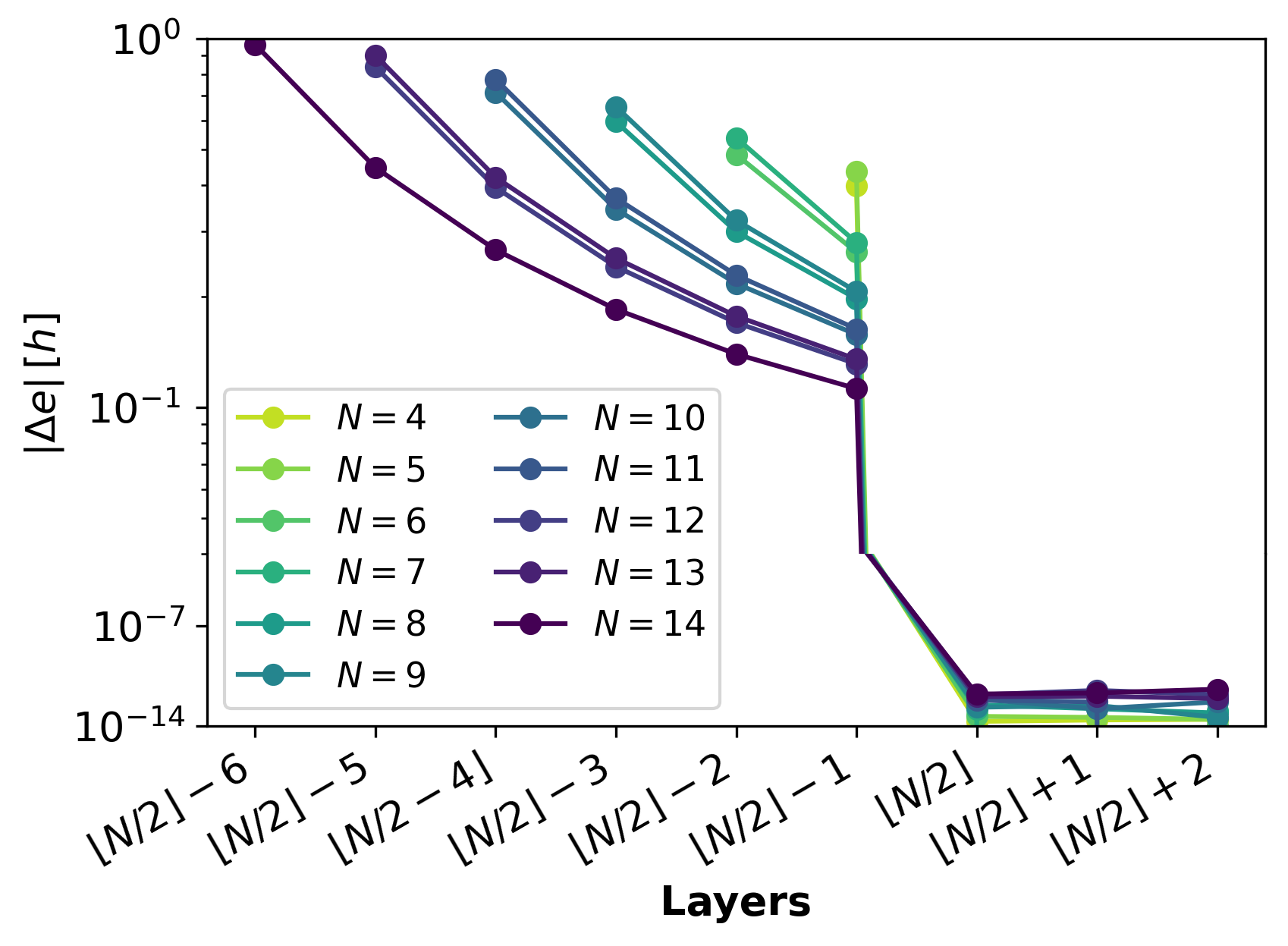
Figure 3: $\Delta\,e=e_{\mathrm{VQE}}-e_{\mathrm{ED}}$, the difference between the ground-state energy per site calculated using the VQE algorithm $e_{\mathrm{VQE}}$ and that computed using exact diagonalization $e_{\mathrm{ED}}$, is shown for the periodic one-dimensional TFIM. $e_{\mathrm{VQE}}$ is computed using $1$ to $\lfloor N/2\rfloor+2$ number of layers of HVA for $N=$3 to 14 spins.

We reconfirmed the sufficiency and necessity of $\lfloor N/2\rfloor$ layers in Fig. 3. It shows the comparison of ground-state energy calculated using the VQE algorithm with that calculated using ED for the ferromagnetic transverse-field Ising chain with periodic boundary conditions at the critical point $J/h=1$. The different curves in the figure show the usage of $1$ to $\lfloor N/2\rfloor+2$ number of layers of HVA for the VQE simulation. The most apparent observation from Fig. 3 is the sudden decrease in the ground-state energy with application of $\lfloor N/2\rfloor$ layers as compared to lower number of layers. Periodic chains reach accurate ground-state energy at $\lfloor N/2\rfloor$ layers for a system with $N$ spins. This implies that the VQE simulation for periodic chains requires only $N$ number of parameters and circuit depth of $2N$ following the brick-wall structure of gates. We observe that this also holds true for the whole polarized phase. To sum up, for the TFIM in one dimension, which is exactly solvable, the ground state is not only approximated but really recovered as soon as the opposing limits $J=0$ and $h=0$ can be expressed by the HVA ansatz. Thinking of other models with two phases, this suggests that this is a good requirement for potential layer ansätze.

3.4 VQE as cluster solver for graphs

The ground-state energy $E_{\mathrm{gs}}$ for finite clusters in Eq. 4 is traditionally calculated using ED in a standard NLCE [51, 52] calculation. Clearly, the ED imposes restrictions on the size of the largest clusters to be included in the NLCE calculation.

In this work, we compute the ground-state energy for finite clusters using the VQE algorithm. It is then embedded back into the infinite lattice using NLCE, hence, approximating the ground-state energy per site in the thermodynamic limit.

NLCE$+$VQE method requires the calculation of ground-state energy for graphs with open boundary conditions. For the purpose of NLCE$+$VQE, we design a new ansatz motivated by HVA with an additional term for boundaries. We call this new ansatz the periodic Hamiltonian variational ansatz (pHVA). For the TFIM given in Eq. 1, this pHVA ansatz is given by

$$U_{N_{l}}^{G}(\vec{\Theta},\vec{\Theta}_{\mathrm{b}})=\prod_{l=1}^{N_{l}}\left[e^{\mathrm{i}\sum_{\nu=1}^{N}\theta^{Z}_{\nu,l}Z_{\nu}}\cdot e^{\mathrm{i}\sum_{<\nu,\mu>}\theta^{XX}_{\nu,\mu,l}X_{\nu}X_{\mu}}e^{\mathrm{i}\sum_{<\nu,\mu>,\mathrm{b}}\theta^{XX}_{\nu,\mu,l,\mathrm{b}}X_{\nu}X_{\mu}}\right],$$ (11)

where $\vec{\Theta}_{\mathrm{b}}$ is the set of parameters for the boundary of the system. In other words, it represents the periodic links in the ansatz for a graph with open boundary conditions. Eq. 11 boils down to the conventional HVA for $\vec{\Theta}_{\mathrm{b}}=0$. Apparent from Eq. (8), the pHVA ansatz for the TFIM is periodic in $\pi$ for every component of the vectors $\vec{\Theta}$ and $\vec{\Theta}_{\mathrm{b}}$.

3.4.1 VQE strategies for finding ground-state energies on graphs

The TFIM on rectangular graphs in general does not possess translational invariance like the periodic clusters in one dimension (section  3.3). In contrast to these periodic chains, where the number of parameters for VQE optimization are $\mathcal{O}(N)$, the graphs for the rectangular graph expansion in one and two dimensions have parameters of the order $\mathcal{O}(N^{2})$. Gradient-based optimization routines become more and more difficult with increasing number of parameters as the optimization gets stuck in local minima more often and more calculations are needed to calculate Hessians and gradients.

However, rectangular graphs in one and two dimensions still possess discrete symmetries. Open transverse-field Ising chains have reflection symmetry. For rectangular graphs in two dimensions the amount of symmetries depends on the graph. These symmetries can be exploited to reduce the number of parameters for VQE simulation to half in one dimension and to at least half in two dimensions. Using these symmetries stabilizes and speeds up the optimization process.

In one dimension, starting the adiabatic optimization from $h=0$ with $\Psi_{\mathrm{gs},\,h=0}$ towards larger values of $h$ works much better than starting from $J=0$ ($\ket{\mathrm{ref}}$ is the polarized state). This way a lot of parameters are already fixed to a good value since it is not trivial to express $\Psi_{\mathrm{gs},\,h=0}$. Although not trivial, we still know how to choose the unitaries to reach this state. However, for rectangular graphs in general, this is different and we do not know the parameters to express $\Psi_{\mathrm{gs},\,h=0}$. For this reason, we modified our strategy and use an approximation to the ground state at the critical point as starting point for our optimization. We obtain this approximation by taking the solution, i.e., the optimized parameters of the periodic systems. We then map these parameters to the initial guess parameters for the optimization of graphs. Before describing the mapping in more detail, let us briefly comment what to do in case the critical point is not yet known. For many systems, upper bounds are easily obtained. For example, the TFIM on hypercubic lattices has the largest value of the critical point at $J/h=1$ in one dimension. Hence, in higher dimensions, the critical point would have the range $[0,1]$. In other situations, the adiabatic optimization can always be performed in the direction of lower or higher ratios of $J/h$ starting from some intermediate coupling ratio.

For the one-dimensional transverse-field Ising chain, it is possible to directly map the parameters from periodic to open chain segments. Since periodic systems are translationally invariant, each layer has two parameters, one for the coupling term and the other for the field term. On the other hand, due to the absence of translational invariance, the open chain segments have $N$ parameters per layer after using the reflection symmetry. We map the optimized parameter for periodic chain corresponding to $\sum_{i}X_{i}X_{i+1}$ term to set it as the initial guess for all the parameters in open chain graphs for $X_{i}X_{i+1}$ for every layer. The same is done for the $Z_{i}$ parameters.

For the square lattice, the corresponding mapping is not straightforward. Different graphs in rectangular-graph expansion have different mapping schemes for initial guess from periodic to open boundary graphs. For chain graphs, we use the aforementioned strategy. Concerning other graphs, the outer boundary of rectangular graphs is a periodic chain in a closed loop. We initialize the parameters corresponding to the outer boundary by the optimized parameters of the periodic chains. The initial values for the edges and vertices inside the closed loop in case of rectangular graphs are set to zero.

4 Calculation of ground-state energy in the thermodynamic limit

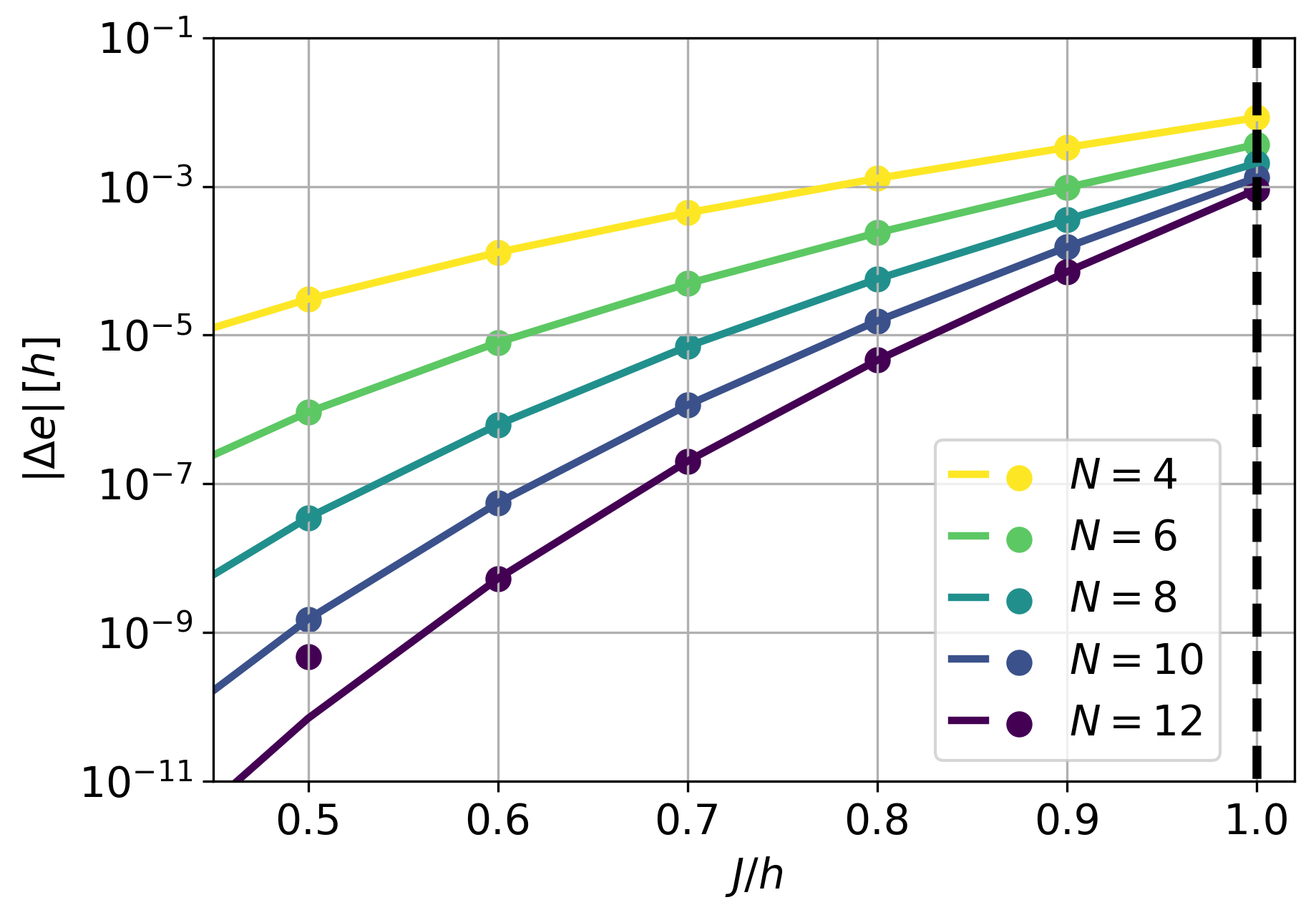
Figure 4: The figure shows the difference between the exact ground-state energy per site of the one-dimensional TFIM [27] and that calculated by NLCE$+$VQE (circles) and NLCE$+$ED (solid lines). $N$ represents different largest cluster sizes included in NLCE calculation. For NLCE$+$VQE we have used $\lceil N/2\rceil$ layers. The vertical dashed line refers to the quantum critical point $J/h=1$.

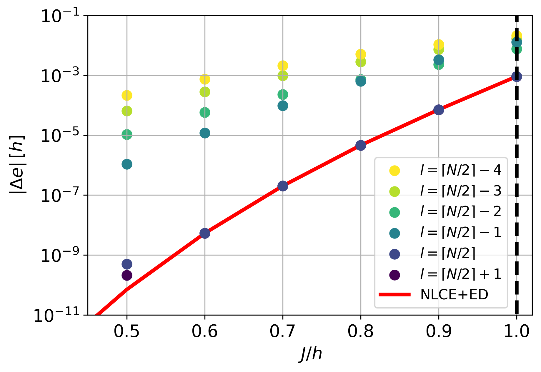
Figure 5: Performance of NLCE$+$VQE for different number of layers $l$ of pHVA for maximal cluster size of 12 spins for the one-dimensional TFIM. The ground-state energy per site is compared against the exact solution [27]. The vertical dashed line refers to the quantum critical point $J/h=1$.

As described in subsection 3.4, we use NLCE with VQE as a cluster solver to approximate the ground-state energy of the TFIM in the polarized phase. We will present results for the model on the chain and on the square lattice for which we use the ground-state energies of rectangular graphs calculated with VQE.

For the one-dimensional TFIM we can always use the exact solution [27] to judge the quality of NLCE$+$VQE. In Fig. 4, we therefore show the difference $\Delta\,e=e_{\mathrm{NLCE}}-e_{\mathrm{exact}}$ between the ground-state energy per site $e_{\mathrm{NLCE}}$ from NLCE and the exact ground-state energy per site $e_{\mathrm{exact}}$ of the transverse-field Ising chain. Here, $N$ is the size of the largest cluster used in the NLCE. The different curves represent the size of the largest cluster used for the NLCE calculation. Note that we always used $\lceil N/2\rceil$ number of layers. The accuracy of NLCE increases as the size of the largest cluster increases, i.e., the ground-state energy per site gets closer to the exact result in the thermodynamic limit for increasing $N$. This is true for the whole polarized phase up to the quantum critical point at $J=h$. At the critical point, the convergence of NLCE is slowest compared to $J/h<1$ which can be directly traced back to the vanishing excitation gap yielding an infinite correlation length. Nevertheless, the accuracy of NLCE$+$VQE and NLCE+ED is $\Delta\,e=9\cdot 10^{-4}$ at $J=h$ using $N=12$. We therefore can conclude that $\lceil N/2\rceil$ layers are sufficient to get quantitative results for the transverse-field Ising chain using NLCE$+$VQE.

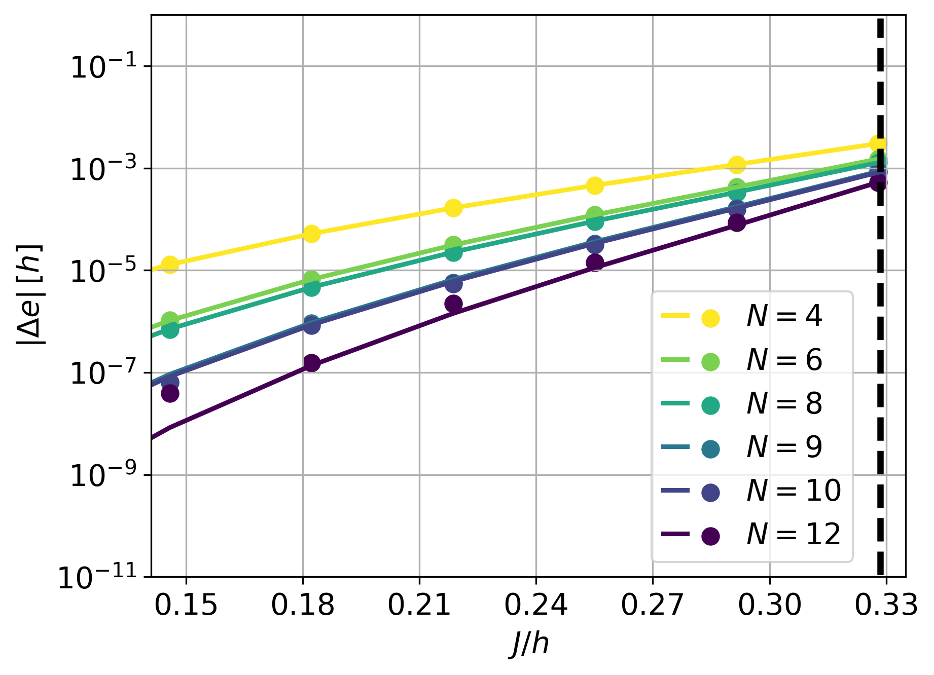
Figure 6: Difference $\Delta\,e$ between the ground-state energy per site calculated with NLCE$+$ED (solid lines) or NLCE$+$VQE (circles) for different maximal number of sites $N$ and that obtained by high-order series expansions about the high-field limit for the TFIM on the square lattice. The NLCE$+$VQE calculation includes all rectangular graphs up to 12 spins. The series have been extrapolated with Padé extrapolations [53]. The vertical dashed line refers to the quantum critical point $J/h\approx 0.328$ [28, 29].

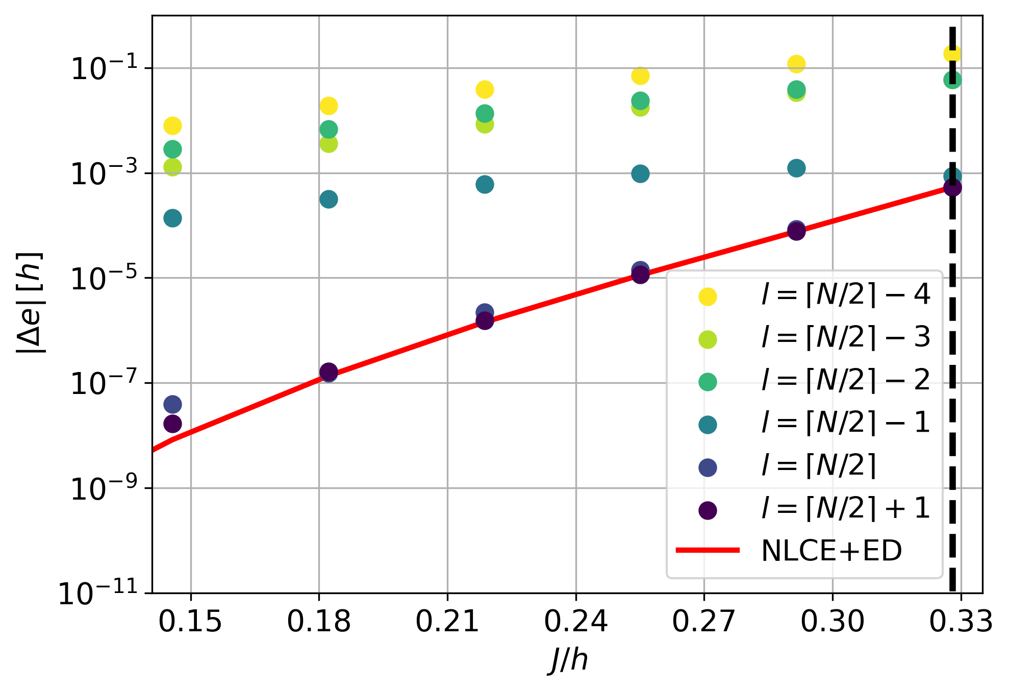
Figure 7: Accuracy of NLCE$+$VQE for a given number of layers $l$ using pHVA for finite clusters with the largest cluster consisting of 12 spins for the TFIM on the two-dimensional square lattice. $\Delta\,e$ is the difference between the energy per site of NLCE$+$VQE and high-order series expansions as described in Fig. 6. The vertical dashed line refers to the quantum critical point $J/h\approx 0.328$ [28, 29].

Next, we discuss the performance of NLCE$+$VQE with the number of layers $l$. The corresponding data for $N=12$ is shown in Fig. 5. Interestingly, the convergence with the number of layers is not smooth, but it rather jumps to larger $\Delta\,e$ when going from $l=\lceil N/2\rceil$ to $l=\lceil N/2\rceil-1$. For example, at the critical point $J=h$, one has $\Delta\,e=9\cdot 10^{-4}$ for $l=\lceil N/2\rceil$, $\Delta\,e=1\cdot 10^{-2}$ for $l=\lceil N/2\rceil-1$, and $\Delta\,e=7\cdot 10^{-3}$ for $l=\lceil N/2\rceil-2$. We emphasize that for $l<\lceil N/2\rceil$ the convergence is not even monotonous, but $\Delta\,e$ is larger for $\lceil N/2\rceil-1$ layers compared to $\lceil N/2\rceil-2$ layers. In contrast, increasing the number of layers to $l>\lceil N/2\rceil$ does not yield any significant further improvement ($\Delta\,e=9\cdot 10^{-4}$ for $l=\lceil N/2\rceil+1$). Altogether, this implies that it is mandatory to take $\lceil N/2\rceil$ layers in order to get convergent results for the one-dimensional TFIM. Physically, it is natural to assume that this can be linked to the numerical finding that the exact ground state of periodic TFIM clusters in one dimensions can be described by this number of layers. Note that this was indeed the motivation for the pHVA ansatz.

Let us now turn to the two-dimensional case where no exact solution is available anymore. We therefore take the ground-state energy from high-order series expansion about the high-field limit [54] as a reference for the full polarized phase up to the quantum critical point $J/h\approx 0.328$ [28, 29]. More specifically, we use Padé extrapolants of order 16 and take their variance as a measure of the uncertainty. We find that this uncertainty is about $10^{-5}$ even at the critical point. In Fig. 6, we therefore show the difference $\Delta\,e=e_{\mathrm{NLCE}}-e_{\mathrm{SE}}$ between the ground-state energy per site $e_{\mathrm{NLCE}}$ from NLCE and the extrapolated ground-state energy per site $e_{\mathrm{SE}}$ from series expansions for the TFIM on the square lattice. As in 1d, $N\leq 12$ is the size of the largest cluster used in the rectangular expansion and $\lceil N/2\rceil$ is taken as the number of layers. The accuracy of NLCE increases with $N$, i.e., the ground-state energy per site gets closer to the extrapolated series expansion result in the thermodynamic limit. Let us stress that the uncertainty of the extrapolation is well below the accuracy of the NLCE. This is true for the whole polarized phase up to the quantum critical point at $J/h=0.328$. At the critical point, the accuracy of NLCE$+$VQE and NLCE+ED is $\Delta\,e=5\cdot 10^{-4}$ at $J=h$ using $N=12$. This also implies that the uncertainty of $e_{\mathrm{SE}}$ from the extrapolations does not impact the current discussion. We therefore find that $\lceil N/2\rceil$ layers is also sufficient to obtain quantitative NLCE$+$VQE results on the square lattice.

Similar to 1d, the accuracy of the NLCE+VQE is not smooth with the number of layers as shown in Fig. 7. Interestingly, for small $J/h$, the jump in $\Delta\,e$ as a function of the number of layers is even larger in two dimensions. In contrast, at the critical point $J/h=0.328$, $\Delta\,e$ of $l=\lceil N/2\rceil-1$ layers is already quite close to the $\Delta\,e$ of $l=\lceil N/2\rceil$ layers, but still a noteworthy energy difference is present. To give numbers: at the critical point, $\Delta\,e=5\cdot 10^{-4}$ for $l=\lceil N/2\rceil$, $\Delta\,e=8\cdot 10^{-4}$ for $l=\lceil N/2\rceil-1$, and $\Delta\,e=5\cdot 10^{-2}$ for $l=\lceil N/2\rceil-2$. Fig. 7 shows that it is important to take $\lceil N/2\rceil$ layers to get convergent results for the polarized phase. Taking even a single layer less in the pHVA ansatz influences the quality of the results significantly. Least deviations are seen at the critical point.

Thus, we can summarize that a ballpark of $N/2$ layers within the pHVA ansatz is required for the graphs in NLCE$+$VQE calculation. This does not impose high demands on quantum computation resources such as the number of gates and circuit depths for the calculation of the ground-state energy of the TFIM in the thermodynamic limit.

5 Conclusions

In this work, we have introduced NLCE+VQE as an efficient tool to treat quantum many-body systems in the thermodynamic limit combining numerical linked-cluster expansions with the quantum-classical VQE algorithm for the calculations on graphs. Here we aim at quantitative results with our approach. In contrast, conventional VQE studies typically target qualitatively correct ground states of finite systems. Our quantitative approach can be significant in many situations, e.g., when different quantum phases are close in energy like in frustrated systems. We are therefore convinced that our approach will be useful in the near future for calculations on real quantum-computing devices. Especially, the rather low requirement of only $\lceil N/2\rceil$ layers of pHVA for the TFIM on clusters of size $N$ is a promising finding.

This convergence without being completely exact on each graph itself also rises questions regarding improving NLCEs, e.g., whether it is essential to consider exact eigenvalues. For excitation energies, this is not true and leads to a non-convergence of NLCEs in the presence of decay processes [25]. It is also related to the stability of NLCE+VQE calculations with respect to errors, which are inevitable when doing calculations on current state-of-the-art quantum computers. With respect to that, it would be desirable to construct an approximation for the unitary of larger graphs by using the solution of smaller subgraphs of this graph. For a conventional NLCE, the logarithm of the transformation $T$, $S=\mathrm{log}\,T$, if properly chosen, is a cluster additive quantity [26], which allows to construct such an approximation. We think it is promising to establish similar considerations for NLCE$+$VQE as it could help become more robust to errors and potentially could help avoid problems with local minima. To generalize the concept of cluster additivity to the HVA circuits is thus an important goal for future research. Additionally, if it is easier to adapt this concept for different ansätze than HVA is a question to be looked into.

Summing up, we calculated the ground-state energy for the unfrustrated TFIM on the chain and the square lattice in the thermodynamic limit using NLCE$+$VQE. We reduced optimization errors by introducing pHVA as a modification of HVA, where periodic links are included for calculations on open clusters. Convergence to conventional NLCE results is demonstrated for $\lceil N/2\rceil$ layers. This implies the scaling of the number of layers is proportional to the correlation length $\xi$ in one dimension, since only two chain segments are required for a given $N$. For the square lattice, the situation is more complicated. However, the quadratic scaling $N^{2}$ of number of rectangular graphs and the linear scaling $l\propto N$ of each cluster are encouraging results. This result promises that NLCE$+$VQE is an efficient tool for quantum calculations only having a polynomial scaling of circuit depth with correlation length. To check if this will also hold for other lattice models is an important task for the future.

One of our next goals is to implement this method on a real quantum device with measurement sampling and determine its accuracy with acceptable quantum errors. We also plan to compute various other observables with the VQE method. For example, one can calculate the ground-state expectation value of the static structure factor for the TFIMs calculated in this paper to determine the location of the quantum critical point. Frustrated systems are challenging systems with potential of exhibiting interesting phenomenons. Another focus of our research in the future is to explore the viability of NLCE$+$VQE method for frustrated lattice models. Finally, it would be very interesting to generalize the NLCE$+$VQE approach to the calculation of excited states.

6 Acknowledgements

The authors thank Michael Hartmann for fruitful discussions on VQE. We also thank Refik Mansuroglu, Lucas Marti and Matthias Mühlhauser for providing their helpful comments and insights. This work was funded by the Deutsche Forschungsgemeinschaft (DFG, German Research Foundation) - Project-ID 429529648 - TRR 306 QuCoLiMa (Quantum Cooperativity of Light and Matter). All authors acknowledge the support by the Munich Quantum Valley, which is supported by the Bavarian state government with funds from the Hightech Agenda Bayern Plus.

References

- [1] F. Verstraete and J. I. Cirac. Matrix product states represent ground states faithfully. Physical Review B - Condensed Matter and Materials Physics, 73(9):1–8, 2006.
- [2] M B Hastings. An area law for one-dimensional quantum systems. Journal of Statistical Mechanics: Theory and Experiment, 2007(08):P08024–P08024, 2007.
- [3] P. A. Whitlock and S. A. Vitiello. Quantum Monte Carlo simulations of solid4He. Lecture Notes in Computer Science (including subseries Lecture Notes in Artificial Intelligence and Lecture Notes in Bioinformatics), 3743 LNCS(1):40–52, 2006.
- [4] Stellan Stlund and Stefan Rommer. Thermodynamic limit of density matrix renormalization. Physical Review Letters, 75(19):3537–3540, 1995.
- [5] G. Vidal. Entanglement renormalization. Physical Review Letters, 99(22):1–4, 2007.
- [6] Alberto Peruzzo, Jarrod McClean, Peter Shadbolt, Man Hong Yung, Xiao Qi Zhou, Peter J. Love, Alán Aspuru-Guzik, and Jeremy L. O’Brien. A variational eigenvalue solver on a photonic quantum processor. Nature Communications, 5(May), 2014.
- [7] Edward Farhi, Jeffrey Goldstone, and Sam Gutmann. A Quantum Approximate Optimization Algorithm. 2022 IEEE 14th International Conference on Wireless Communications and Signal Processing, WCSP 2022, pages 804–808, nov 2014.
- [8] Scott E. Smart and David A. Mazziotti. Quantum Solver of Contracted Eigenvalue Equations for Scalable Molecular Simulations on Quantum Computing Devices. Physical Review Letters, 126(7):70504, 2021.
- [9] Jules Tilly, Hongxiang Chen, Shuxiang Cao, Dario Picozzi, Kanav Setia, Ying Li, Edward Grant, Leonard Wossnig, Ivan Rungger, George H. Booth, and Jonathan Tennyson. The Variational Quantum Eigensolver: A review of methods and best practices, volume 986. 2022.
- [10] Jarrod R McClean, Jonathan Romero, Ryan Babbush, and Alán Aspuru-Guzik. The theory of variational hybrid quantum-classical algorithms. New Journal of Physics, 18(2), 2016.
- [11] M. F. Sykes, J. W. Essam, B. R. Heap, and B. J. Hiley. Lattice constant systems and graph theory. J. Math. Phys., 7(9):1557–1572, 1966.
- [12] Jaan Oitmaa, Chris Hamer, and Weihong Zheng. Series Expansion Methods for Strongly Interacting Lattice Models. Cambridge University Press, Cambridge, 2006.
- [13] Marcos Rigol, Tyler Bryant, and Rajiv R.P. Singh. Numerical linked-cluster approach to quantum lattice models. Physical Review Letters, 97(18):3–6, 2006.
- [14] Baoming Tang, Ehsan Khatami, and Marcos Rigol. A short introduction to numerical linked-cluster expansions. Computer Physics Communications, 184(3):557–564, 2013.
- [15] Marcos Rigol and Rajiv R.P. Singh. Magnetic susceptibility of the kagome antiferromagnet ZnCu3(OH)6Cl2. Physical Review Letters, 98(20):2–5, 2007.
- [16] Ehsan Khatami, Rajiv R.P. Singh, and Marcos Rigol. Thermodynamics and phase transitions for the Heisenberg model on the pinwheel distorted kagome lattice. Physical Review B - Condensed Matter and Materials Physics, 84(22):1–6, 2011.
- [17] Ehsan Khatami, Joel S. Helton, and Marcos Rigol. Numerical study of the thermodynamics of clinoatacamite. Physical Review B - Condensed Matter and Materials Physics, 85(6):1–7, 2012.
- [18] R. Applegate, N. R. Hayre, R. R.P. Singh, T. Lin, A. G.R. Day, and M. J.P. Gingras. Vindication of Yb 2Ti 2O 7 as a model exchange quantum spin ice. Physical Review Letters, 109(9):1–5, 2012.
- [19] Elmer Guardado-Sanchez, Peter T. Brown, Debayan Mitra, Trithep Devakul, David A. Huse, Peter Schauß, and Waseem S. Bakr. Probing the Quench Dynamics of Antiferromagnetic Correlations in a 2D Quantum Ising Spin System. Physical Review X, 8(2):21069, 2018.
- [20] Krishnanand Mallayya and Marcos Rigol. Quantum Quenches and Relaxation Dynamics in the Thermodynamic Limit. Physical Review Letters, 120(7):70603, 2018.
- [21] Baoming Tang, Deepak Iyer, and Marcos Rigol. Thermodynamics of two-dimensional spin models with bimodal random-bond disorder. Physical Review B - Condensed Matter and Materials Physics, 91(17):1–9, 2015.
- [22] M. D. Mulanix, Demetrius Almada, and Ehsan Khatami. Numerical linked-cluster expansions for disordered lattice models. Physical Review B, 99(20):205113, 2019.
- [23] Colin J. Morningstar and Marvin Weinstein. Contractor renormalization group technology and exact Hamiltonian real-space renormalization group transformations. Physical Review D - Particles, Fields, Gravitation and Cosmology, 54(6):4131–4151, 1996.
- [24] H. Y. Yang and K. P. Schmidt. Effective models for gapped phases of strongly correlated quantum lattice models. Epl, 94(1), 2011.
- [25] K. Coester, S. Clever, F. Herbst, S. Capponi, and K. P. Schmidt. A generalized perspective on non-perturbative linked-cluster expansions. Epl, 110(2), 2015.
- [26] Max Hörmann and Kai P. Schmidt. Projective cluster-additive transformation for quantum lattice models. SciPost Physics, 15(3):1–26, 2023.
- [27] Pierre Pfeuty. The one-dimensional Ising model with a transverse field. Annals of Physics, 57(1):79–90, 1970.
- [28] H. X. He, C. J. Hamer, and J. Oitmaa. High-temperature series expansions for the (2+1)-dimensional Ising model. Journal of Physics A: Mathematical and General, 23(10):1775–1787, 1990.
- [29] S. Hesselmann and S. Wessel. Thermal Ising transitions in the vicinity of two-dimensional quantum critical points. Physical Review B, 93(15):1–11, 2016.
- [30] M. Powalski, K. Coester, R. Moessner, and K. P. Schmidt. Disorder by disorder and flat bands in the kagome transverse field Ising model. Physical Review B - Condensed Matter and Materials Physics, 87(5):1–10, 2013.
- [31] R. Moessner and S. L. Sondhi. Ising models of quantum frustration. Physical Review B - Condensed Matter and Materials Physics, 63(22):1–19, 2001.
- [32] Martin P. Gelfand. Series expansions for excited states of quantum lattice models. Solid State Communications, 98(1):11–14, 1996.
- [33] Marcos Rigol, Tyler Bryant, and Rajiv R.P. Singh. Numerical linked-cluster algorithms. I. Spin systems on square, triangular, and kagomé lattices. Physical Review E - Statistical, Nonlinear, and Soft Matter Physics, 75(6), 2007.
- [34] A. C. Irving and C. J. Hamer. Methods in hamiltonian lattice field theory (II). Linked-cluster expansions. Nuclear Physics, Section B, 230(3):361–384, 1984.
- [35] Walter Ritz. Über eine neue Methode zur Lösung gewisser Variationsprobleme der mathematischen Physik, 1909.
- [36] Dave Wecker, Matthew B. Hastings, and Matthias Troyer. Progress towards practical quantum variational algorithms. Physical Review A - Atomic, Molecular, and Optical Physics, 92(4):1–10, 2015.
- [37] M. Cerezo, Akira Sone, Tyler Volkoff, Lukasz Cincio, and Patrick J. Coles. Cost function dependent barren plateaus in shallow parametrized quantum circuits. Nature Communications, 12(1), 2021.
- [38] Lennart Bittel and Martin Kliesch. Training Variational Quantum Algorithms Is NP-Hard. Physical Review Letters, 127(12):120502, 2021.
- [39] Roeland Wiersema, Cunlu Zhou, Yvette De Sereville, Juan Felipe Carrasquilla, Yong Baek Kim, and Henry Yuen. Exploring Entanglement and Optimization within the Hamiltonian Variational Ansatz. PRX Quantum, 1(2), oct 2020.
- [40] Ruoshui Wang, Timothy H. Hsieh, and Guifré Vidal. Bang-bang algorithms for quantum many-body ground states: A tensor network exploration. Physical Review B, 106(19):1–7, 2022.
- [41] Roeland Wiersema, Cunlu Zhou, Yvette De Sereville, Juan Felipe Carrasquilla, Yong Baek Kim, and Henry Yuen. Exploring Entanglement and Optimization within the Hamiltonian Variational Ansatz. PRX Quantum, 1(2):1–16, 2020.
- [42] Chae-Yeun Park and Nathan Killoran. Hamiltonian variational ansatz without barren plateaus. (2):1–17, 2023.
- [43] Antonio A. Mele, Glen B. Mbeng, Giuseppe E. Santoro, Mario Collura, and Pietro Torta. Avoiding barren plateaus via transferability of smooth solutions in a Hamiltonian variational ansatz. Physical Review A, 106(6):1–7, 2022.
- [44] Elbio Dagotto and Adriana Moreo. Improved Hamiltonian variational technique for lattice models. Physical Review D, 31(4):865–870, 1985.
- [45] Baptiste Anselme Martin, Pascal Simon, and Marko J. Rančić. Simulating strongly interacting Hubbard chains with the variational Hamiltonian ansatz on a quantum computer. Physical Review Research, 4(2):1–11, 2022.
- [46] Kouhei Nakaji and Naoki Yamamoto. Expressibility of the alternating layered ansatz for quantum computation. Quantum, 5:1–20, 2021.
- [47] Edward Farhi, Jeffrey Goldstone, Sam Gutmann, and Michael Sipser. Quantum Computation by Adiabatic Evolution. 2000.
- [48] D. C. Sorensen. Trust Region Modification. Society for Industrial and Applied Mathematics, 19(2):409–426, 1982.
- [49] Luigi Grippo and Marco Sciandrone. Line Search Methods. UNITEXT - La Matematica per il 3 piu 2, 152:187–227, 2023.
- [50] Glen Bigan Mbeng, Rosario Fazio, and Giuseppe Santoro. Quantum Annealing: a journey through Digitalization, Control, and hybrid Quantum Variational schemes. 2019.
- [51] Dominik Ixert and Kai Phillip Schmidt. Nonperturbative linked-cluster expansions in long-range ordered quantum systems. Physical Review B, 94(19):1–16, 2016.
- [52] Sébastien Dusuel, Michael Kamfor, Kai Phillip Schmidt, Ronny Thomale, and Julien Vidal. Bound states in two-dimensional spin systems near the Ising limit: A quantum finite-lattice study. Physical Review B - Condensed Matter and Materials Physics, 81(6), 2010.
- [53] C Domb, M S Green, and J L Lebowitz. Phase Transitions and Critical Phenomena. Number v. 13 in Phase Transitions and Critical Phenomena. Academic Press, 1989.
- [54] H. X. He, C. J. Hamer, and J. Oitmaa. High-temperature series expansions for the (2+1)-dimensional Ising model. Journal of Physics A: Mathematical and General, 23(10):1775–1787, 1990.