Recovering the E and B-mode CMB polarization
at sub-degree scales with neural networks

Abstract

Aims.

Methods.

Results.

Abstract

Context. Recovering the polarized cosmic microwave background (CMB) is crucial for shading light on the exponential growth of the very early Universe called Cosmic Inflation. In order to recover that signal, methods with different characteristics should be developed and optimized.

Aims. We aim to use a neural network called the CMB extraction neural network (CENN) and train it for recovering the E and B modes of the CMB at sub-degree scales.

Methods. We train the network with realistic simulations of the 100, 143 and 217 GHz channels of Planck, which contain the CMB, thermal dust, synchrotron emission, point sources and instrumental white noise. Each simulation is formed by three patches of 256$\times$256 pixels with a 90 arcsec pixel value at latitude $|b|>30^{\circ}$. We make several trainings sets with 10000 simulations each: 30, 25 and 20 arcmin resolution patches at the same position in the sky. After being trained, CENN is able to recover the CMB signal at 143 GHz in $Q$ and $U$ patches. Then, we use NaMaster for estimating the average $EE$ and $BB$ power spectrum for each input and output patches in the validation dataset, as well as the difference between input and output power spectra and the residuals. For generalization, we also test the methodology using a different foreground model at 5 arcmin resolution without noise.

Results. We recover the CMB at 30, 25 and 20 arcmin train resolution: for the E-mode, we generally found residuals bellow the input signal at all scales. In particular, we found a value of about $10^{-1}$  $\mu K\hskip 1.0pt^{2}$ at $l<200$, decreasing below $10^{-2}$  $\mu K\hskip 1.0pt^{2}$ at smaller scales. For the B-mode, we similarly recover the CMB with residuals between $10^{-2}$ and $10^{-3}$  $\mu K\hskip 1.0pt^{2}$. We also train the network with 5 arcmin Planck simulations without noise, obtaining clearly better results with respect the previous cases. When tested the network performance with a different foreground model, the recovery is similar, although B-mode residuals increase above the input signal. In general, we found that, the network performs better when training with the same resolution used for testing.

Conclusions. Based on these results, CENN seems to be a promising, alternative and flexible tool for recovering both $E$ and $B$-mode polarization at sub-degree scales. Due to its performance at middle and small scales, it could be useful for its use in ground-base experiments such as POLARBEAR, SO and CMB-S4. Once extending its applicability at all sky, it could be an alternative component separation method for LiteBIRD satellite in order to help in the search for primordial B-modes.

1 Introduction

The cosmic microwave background (CMB) is believed to be the afterglow of the Big Bang, dating back to about 380000 years after the birth of the Universe originating when photons decoupled from baryons and it became transparent to light. It is a key probe of the early times and it is known to be partially linear polarized, which can be described by the Stokes Q and U parameters (Hu & White, 1997). However, the polarization can also be decomposed into gradient and curl modes, known as E and B modes respectively. This decomposition is typically done using the total angular momentum approach, as proposed by Kamionkowski et al. (1997) and Zaldarriaga & Seljak (1997). The E modes are associated with scalar (density) perturbations in the early universe, while the B modes are sourced by tensor (gravitational) perturbations, which arise from the gravitational lensing of the CMB by intervening large-scale structure, as so as inflationary gravitational waves.

The B-mode polarization of the CMB is an important signal because it can provide information about the presence of primordial gravitational waves. They are a direct probe of inflationary cosmological models, which propose that the Universe underwent a period of exponential expansion in its first stages (Guth 1981, Linde 1982). The strength of the tensor perturbations is characterized by the tensor-to-scalar ratio parameter, $r$, which is defined as the ratio of the amplitudes of the tensor and scalar perturbations. Several inflationary models predict different values of $r$, which can be observationally constrained by observations of the CMB (Baumann, 2009).

Over the past few years, different experiments have reconstructed the power spectrum of the E modes and their correlation with the total intensity field, particularly the Planck satellite (Planck Collaboration V, 2020), which recovered that spectrum up to sub-degree angular scales. However, the B modes remain much more challenging to detect, as they are expected to be much weaker than the E modes. Currently, the upper limit on the tensor-to-scalar ratio is $r<0.036$ at 95% confidence level using Planck, WMAP and BICEP/Keck Array 2018 data (Bicep/Keck Collaboration et al., 2021). However, upcoming experiments such as LiteBIRD and CMB-S4 are expected to improve this limit significantly, achieving sensitivities of $\sigma(r)$ = 0.001 (LiteBIRD Collaboration et al., 2022) and $\sigma(r)$ = 0.0005 (Abazajian et al., 2022) respectively.

Considering a target value for $r$ between $10^{-3}$ and $10^{-4}$, the detection of B modes in the CMB polarization is a challenging task due to several systematic uncertainties and contamination from foregrounds (Baccigalupi 2003, Krachmalnicoff et al. 2016), which are microwave Galactic emissions and extragalactic sources. Galactic foregrounds are mainly divided into thermal dust (see Hensley & Draine (2021) for a comprehensive review) and synchrotron emission (Krachmalnicoff et al. 2018, Fuskeland et al. 2021). Extragalactic sources are principally blazars with their jets aligned in the line of sight of the instrument, and their emission is highly linear polarized due to synchrotron radiation emitted from their active galactic nuclei (Tucci & Toffolatti 2012, Puglisi et al. 2018).

Therefore, ongoing research is focused on improving not only the sensitivity of future experiments but developing new techniques for foreground removal, including the use of multi-frequency observations and sophisticated component separation methods. Some of them are described in the works by Leach et al. (2008) and Fuskeland et al. (2023), and vary between parametric Bayesian frameworks such as Commander (Eriksen et al., 2008), SMICA (Delabrouille et al., 2003) or FGBuster (Stompor et al. 2009, Puglisi et al. 2022), template-based methods such as SEVEM (Fernández-Cobos et al., 2012), moment-expansion methods (Chluba et al. 2017, Vacher et al. 2022) and minimum variance methods such as NILC (Delabrouille et al., 2009), GNILC (Remazeilles et al., 2011) and cMILC (Remazeilles et al., 2021).

Machine learning (ML) has become increasingly important in various fields due to its ability to learn patterns and make predictions from large amounts of data. One of the most popular ML models are neural networks, which can learn non-linear behaviors from data (Goodfellow et al., 2016). They are composed of interconnected computational units called neurons, which are organized in layers. The learning process of a neural network is an optimization problem where the objective is to minimize a loss function at the end of their architecture. The training of a neural network involves the flow of information from the input layer through the hidden ones and towards the output layer. Each neuron applies a non-linear activation function to the information it receives, allowing only certain information to pass through. After the output layer, the loss function is calculated using a target value in the data called the label. The backpropagation algorithm (Rumelhart et al., 1986) is then used to update the weights and biases of the neurons, allowing the network to improve its predictions. This process is repeated over several epochs until the loss function is minimized, indicating that the network has learned the patterns in the data.

Convolutional neural networks (CNN) have become a powerful tool in image analysis and recognition due to their ability to learn and extract features from images. In a CNN, each layer produces a convolution between the input image and a set of filters in order to produce feature maps. The filters consist of small matrices of weights called kernels that slide over the input image, allowing the network to learn different features at different positions in the image. Then, during the backpropagation process, both the filters and the kernels become updated. Furthermore, fully-convolutional neural networks (FCN) are an evolution of CNN that have been extensively used for image segmentation tasks. They are formed by a series of convolutional layers that process the input image, followed by layers that perform deconvolutions to produce an output segmentation map of the same size as the input image. They have shown great success in various image segmentation tasks, including medical and object detection tasks.

Recently, neural networks have been applied to various problems in astrophysics, including component separation with remarkable accuracy and efficiency (Petroff et al. 2020, Jeffrey et al. 2022, Casas et al. 2022a, Wang et al. 2022, Yan et al. 2023). Good performance have been also achieved in recognizing foreground models (Farsian et al., 2020), detecting extragalactic point sources in single- (Bonavera et al., 2021) and multi-frequency (Casas et al., 2022b) total intensity Plank-like data and for constraining their polarization flux densities and angles using polarization Planck data (Casas et al., 2023). Also, they have been used for simulating dust foregrounds (Krachmalnicoff & Puglisi, 2021) or inpainting foreground maps (Puglisi & Bai, 2020).

In this work, we aim to train the cosmic microwave background extraction neural network (CENN) presented in Casas et al. (2022a) with polarization data for recovering the CMB signal in patches of the sky. The work is organized as follows: Section 2 describes several simulated datasets we use for training and validating the network and Section 3 describes the adopted methodology. The results are presented in Section 4 and our conclusions can be seen in Section 5.

2 Simulations

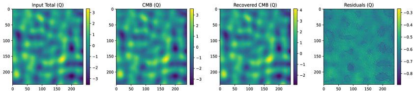
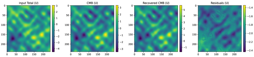
Figure 1: Example of one simulation used for training CENN in $Q$ (top row) and $U$ (bottom row) polarization at 30 arcmin resolution. The left column shows the input patch formed by all the emissions, the second one represents only the CMB signal, used for minimizing the loss function during training. The third column shows the output CMB after validating CENN and the fourth one shows the residual patch, which is computed as the difference between input and output CMB. The units in all the patches are $\mu K_{CMB}$.

Our training, validation and testing datasets are formed by realistic simulations of the microwave $Q$ and $U$ sky at 100, 143 and 217 GHz as seen by Planck. They were downloaded from the Planck Legacy Archive website . The $N_{side}=2048$ maps were cutted using the methodology described in Krachmalnicoff & Puglisi (2021) in quadratic patches of 256$\times$256 pixels, with a pixel size of 90 arcsec, which imply patches of 6.4 deg² of area. Each signal in the patch is smoothed with gaussian filters of 30, 25 and 20 arcmin, depending on the test dataset, in order to improve the low signal-to-noise ratio of each pixel due to the low sensitivity of the Planck instrument.

Each patch is formed by a lensed CMB signal, random white instrumental noise at Planck levels, that is, 1.96, 1.17 and 1.75 $\mu K_{CMB}$ at 100, 143 and 217 GHz respectively (before smoothing the data) and Galactic and extragalactic foregrounds. The Galactic foregrounds are thermal dust and synchrotron emission. The first one, following the PLA documentation, is simulated with a realization of the Vansyngel et al. (2017) model at 353 GHz and extrapolated to the lower frequencies used in this work by using Planck 2015 dust maps and Planck 2013 dust spectral index maps. The synchrotron emission, also following the PLA documentation. is simulated by following a power law scaling with a spatially varying spectral index for such emission. Therefore, they are similar to the d6s1 foreground model of the Python Sky Model (PySM, Thorne et al. (2017), Zonca et al. (2021)). The only extragalactic foreground taken into account are point sources, which are injected into each patch by following the total intensity C2Ex model from Tucci et al. (2011) and the software CORRSKY (González-Nuevo et al., 2005) and extrapolating their polarization by assuming a log-normal distribution with $\mu=1.0$ and $\sigma=0.7$ parameters at 143 GHz from Bonavera et al. (2017).

Additionally, we tested CENN against simulations with a different foreground model (see Section 4.4). In that case, the test dataset includes thermal dust with an emissivity varying spatially on degree scales and synchrotron emission index steepening off the Galactic plane, which is exactly the d4s2 foreground model downloaded from the PySM.

Therefore, we simulate three kind of datasets for training and testing the network. The first one, used for training, is formed by 10000 simulations. The second one, formed by 1000 simulations, is used for validating the network during training. The best trained model obtained from this validation dataset (the one with the lower loss) is then used for testing the network against new data. In particular, we do four trainings, one at 30 arcmin resolution, another one at 25 arcmin, another one at 20 arcmin and the last one at 5 arcmin without noise, having several validation and test sets for each case. An example of the input and label $Q$ and $U$ simulated patches at 143 GHz at 30 arcmin is shown in Fig. 1, first two columns. An example of the multi-frequency set of patches for the same simulation is shown in Fig. 2.

3 Methodology

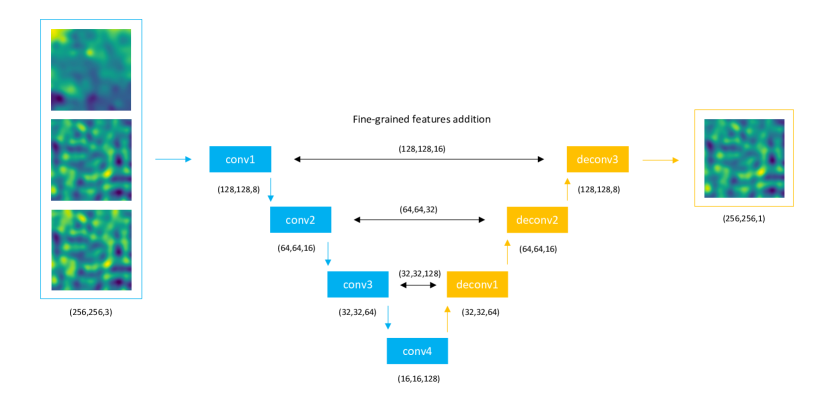
Figure 2: Architecture of CENN. It has four convolutional blocks connected to other four deconvolutional ones, which are trained to read 3 input images of the microwave sky and recovery the CMB signal of the central frequency channel (in this case corresponding to 143 GHz).

In this work, we have developed a methodology based on fully-convolutional neural networks for recovering the polarized CMB signal from noisy background patches of the sky. The details of how these kind of neural networks are able to perform image segmentation on multi-frequency data are explained mathematically and physically in Goodfellow (2010) and Casas et al. (2022a) respectively, and the reader is encouraged to looking for these works.

The neural network is trained to read a set of three patches of the microwave sky and output a patch with only the CMB signal. The architecture, represented in Fig. 2, is used for training simultaneously both $Q$ and $U$ data. The network is formed by four convolutional blocks with 8, 2, 4 and 2 kernels of sizes of 9, 9, 7 and 7, respectively. The number of filters is 8, 16, 64 and 128, respectively. Each layer has a subsampling factor of 2 and a padding type ”Same” for adding space around the input data or the feature map in order to deal with possible loss in width and/or height dimension in the feature maps after having applied the filters. The convolutional blocks are connected to four deconvolutional ones to help the network to predict low-level features by taking high-level features into account, previously inferred by the convolutional blocks, as explained in Wei et al. (2021) and Casas et al. (2022a). The deconvolutional blocks have 2, 2, 2 and 4 kernels of sizes of 3, 5, 7 and 7, respectively. The number of filters is 64, 16, 8, and 1 with the same subsampling and padding type than the convolutional ones. In all layers, the activation function is leaky ReLU.

In the first convolutional block, CENN reads three patches at 100, 143 and 217 GHz of the polarized microwave sky, splitting the information into its first 8 feature maps after convolving it with randomly initialized filters and weights. The information allowed to pass by the activation function function is convolved by the next blocks. Then, three additional deconvolutional blocks, subsequently connected to the convolutional ones, as shown in Fig 2, segmentate the CMB signal from 128 small feature maps. A fourth deconvolutional block is added to reconstruct the CMB signal from 8 final feature maps to a patch of the same dimension than the input ones.

In that final layer, a Mean Squared Error loss function

$$MSE\hskip 1.0pt=\hskip 1.0pt\frac{1}{2}\hskip 1.0pt|\hskip 1.0pty\hskip 1.0pt-\hskip 1.0pty^{\prime}\hskip 1.0pt|^{2}$$ (1)

is introduced, where $y$ is a matrix formed by the predicted CMB pixel values and $y^{\prime}$ is the CMB signal at 143 GHz. This function computes a loss, which is then used to estimate a gradient value, which is needed for updating both kernels and filters on each layer of the architecture using the backpropagation and the AdaGrad optmizer. All the information forming the train dataset flows forward and backward the network with a batch size of 8. Once 500 epochs are completed, the training is complete and the CMB could be disentangled from the total input sky patches.

4 Results

Once trained, CENN is able to read three patches of the sky and produce an output image with the clean CMB patch with the same dimensions of the training ones. In this section, the network is tested with similar and different conditions with respect to the training ones. More particularly, in Section 4.1, the network is trained and tested with data smoothed at 30 arcmin. Section 4.2 shows the comparison between training the network at 25 arcmin and training at 30 arcmin, being both networks tested at 25 arcmin. Section 4.3 presents the same analysis but for training and testing at 20 arcmin resolution. It should be noted that increasing the resolution allows to reach higher multipoles, although decreasing the signal-to-noise ratio: using 30 arcmin allows us to reach $l\sim 600$, a resolution of 25 arcmin allows to achieve $l\sim 700$ and 20 arcmin to get to about $l\sim 800$. Section 4.4 shows how the model recovers the CMB at smaller angular scales by training and testing at 5 arcmin-Planck data without instrumental noise, which can be also seen as an approximation to future CMB experiments. In the same section, we also change the foreground model of the simulations for testing generalization.

4.1 Training at 30 arcmin

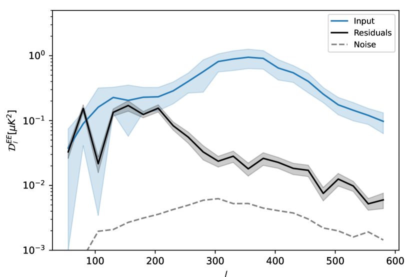
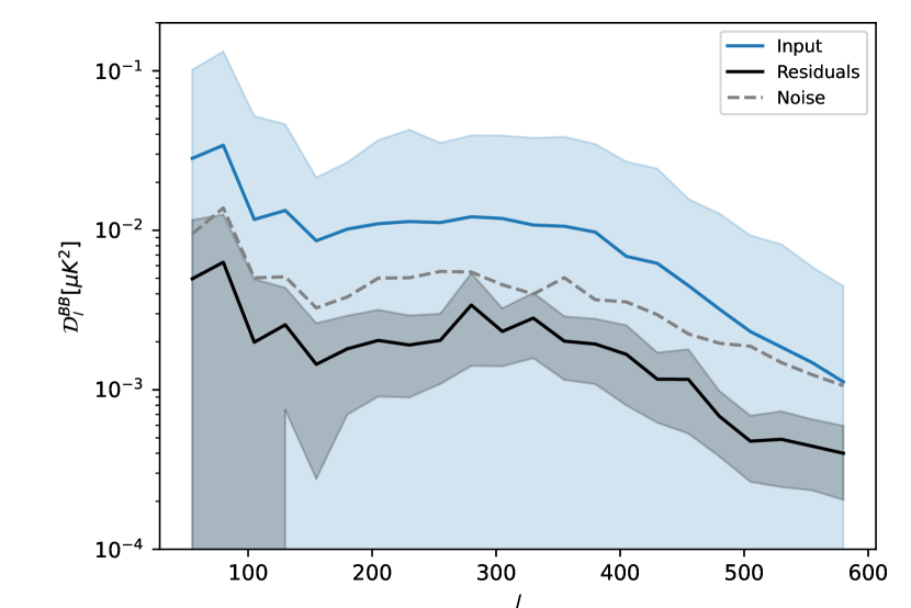
Figure 3: EE and BB residuals after training CENN at 30 arcmin resolution and tested at the same resolution. Left panel: EE power spectra in the input simulations (blue line) and residual patch average power spectra from CENN at 30 arcmin (black line). Right panel: the same but for the B-mode. In all cases, coloured areas shown the standard deviation of each bin, considered as the uncertainty of the model. Grey dashed line shows the higher instrumental noise levels seen by CENN.

Once the network has been trained at 30 arcmin, we apply it to a testing set of simulations, different from the training set. It outputs 1000 patches containing its prediction of the CMB. $Q$ and $U$ CMB simulated and output patches are then combined using NaMaster for analyzing the E and B-mode power spectra.

We use the methodology proposed in (Krachmalnicoff & Puglisi, 2021) to extract the patches for the test set. However, we realize that this procedure leaves a clear E-to-B leakage, when it is applied to maps encoding CMB signal only. In fact, (Krachmalnicoff & Puglisi, 2021) employed it to Galactic emission maps and they did not find no leakage because the $E-$ and $B-$ mode signal is comparable specifically for thermal dust. We find that the leakage reduces sensibly for patches smaller $\Delta\theta\lesssim 7$ and we therefore decide to use square $256\times 256$ patches. It should be noted that, due to the limited size of the patch, the signal at large scales, below $l<50$, cannot be recovered with our methodology. In order to recover larger scales, it should be better to use approaches such as the one in Wang et al. (2022) and Yan et al. (2023), or extending the neural network performance at all sky by using different methodologies such those proposed in Krachmalnicoff & Tomasi (2019) or Perraudin et al. (2019).

In order to represent the results, we have rebinned the power spectra between $l=50$ and $l=$ 600, 700 and 800 depending on the smoothing we use for testing the network (30, 25 and 20 arcmin, respectively). For each bin, the mean and the standard deviation are used to represent the signal and its uncertainty. The analysis present in this work is mainly due attending to the residuals power spectra, which is computed as the average of the power spectrum of the residual patch (formed as the difference between input and recovered ones). More results about the difference between input and recovered signal is described in the Appendix A.

Fig 3 shows the EE and BB power spectra of the residuals in black, compared against the input power spectra in blue. The respective uncertainties are represented as coloured areas. We also represent as grey dashed lines the highest instrumental noise level between the three channels seen by CENN when testing, corresponding to the 100 GHz channel (Planck Collaboration et al., 2018).

As shown in the left panel, CENN accurately recovers the E-mode since the input signal is generally above the residuals. Moreover, at large scales ($l<200$), residuals are approximately $10^{-1}$ $\mu K\hskip 1.0pt^{2}$, decreasing to $10^{-2}$ $\mu K\hskip 1.0pt^{2}$ while increasing the scale to $l>500$. At smaller scales, residuals are below $10^{-2}$ $\mu K\hskip 1.0pt^{2}$. In this case, attending to the noise levels, residuals are mainly artifacts generated by CENN due to Galactic contamination.

On the other hand, as shown in the right panel, the performance is similar for the B-mode: in that case, residuals are about $2\times 10^{-3}$ $\mu K\hskip 1.0pt^{2}$ for $l<400$, decreasing to $5\times 10^{-4}$ $\mu K\hskip 1.0pt^{2}$ at $l>500$, that is, generally one order of magnitude below the input signal, represented in blue. In fact, as shown, noise levels are above the residuals at all scales, showing that instrumental noise is not affecting CENN when recovering the B-mode.

4.2 Training at 25 arcmin

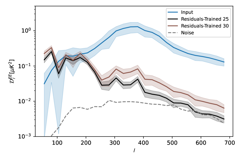
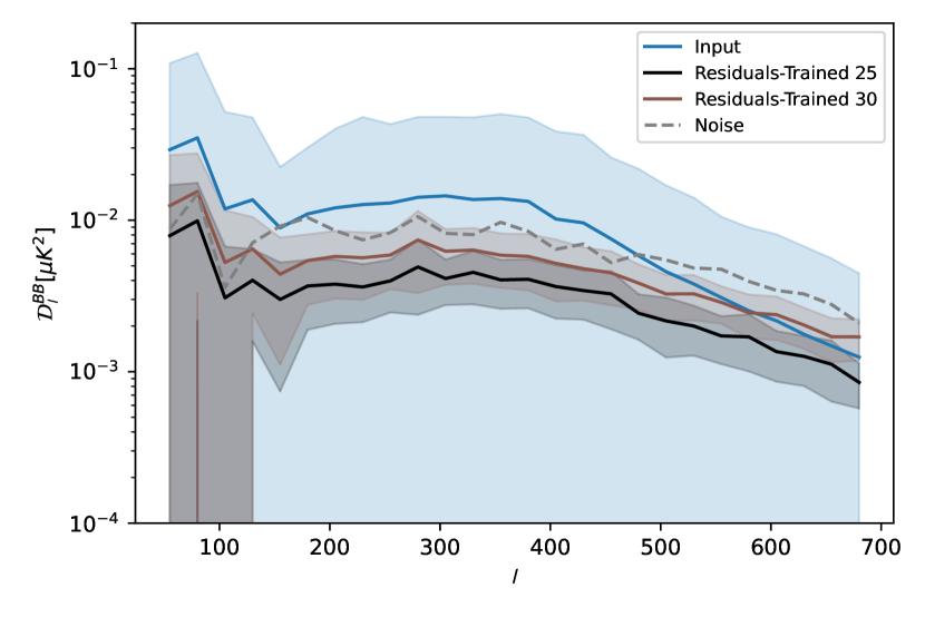
Figure 4: EE and BB residuals after training CENN at 25 and 30 arcmin resolution and tested at 25 arcmin. Left panel: EE power spectra in the input simulations (blue line), residual patch average power spectra from CENN at 25 (black line) and 30 arcmin (brown line). Right panel: the same but for the B-mode. In all cases, coloured areas shown the standard deviation of each bin, considered as the uncertainty of the model. Grey dashed line shows the higher instrumental noise levels seen by CENN.

After analyzing how CENN performs at 30 arcmin, we decide to study its performance when training at a lower resolution. In this section, we create new train and test datasets with 10000 and 1000 simulations, respectively at 25 arcmin resolution. Firstly, we apply the network of the previous section trained with 30 arcmin to these patches, and then we compare its performance with the network trained with 25 arcmin data.

Figure 4 represent EE and BB residuals power spectra, being the E-mode on the left panel and the B-mode on the right one. Again, the comparison between both input and recovered signals is described in the Appendix A.

We derive similar conclusions as in the previous case: E-mode residuals are generally lower than the input signal (in blue), with a value of about $10^{-1}$ $\mu K\hskip 1.0pt^{2}$ at $l<200$, descending to $10^{-2}$ $\mu K\hskip 1.0pt^{2}$ while decreasing the scale. The B-mode is also accurately recovered, especially at $l<600$, when residuals are lower than the input signal. As shown, the network is more sensitive to noise (represented as grey dashed line) at high ($l<100$) and small ($500<l<700$) scales. Furthermore, residuals are generally lower in both modes when training the network at 25 arcmin resolution with respect to the 30 arcmin case. Threfore, it seems to be better to train the network at the same conditions than for testing while the instrumental noise level is still lower than the input signal.

4.3 Training at 20 arcmin

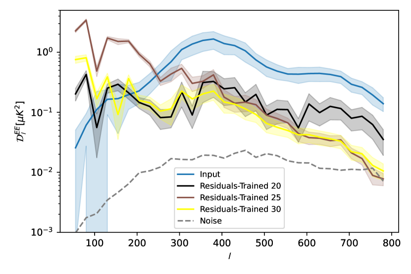
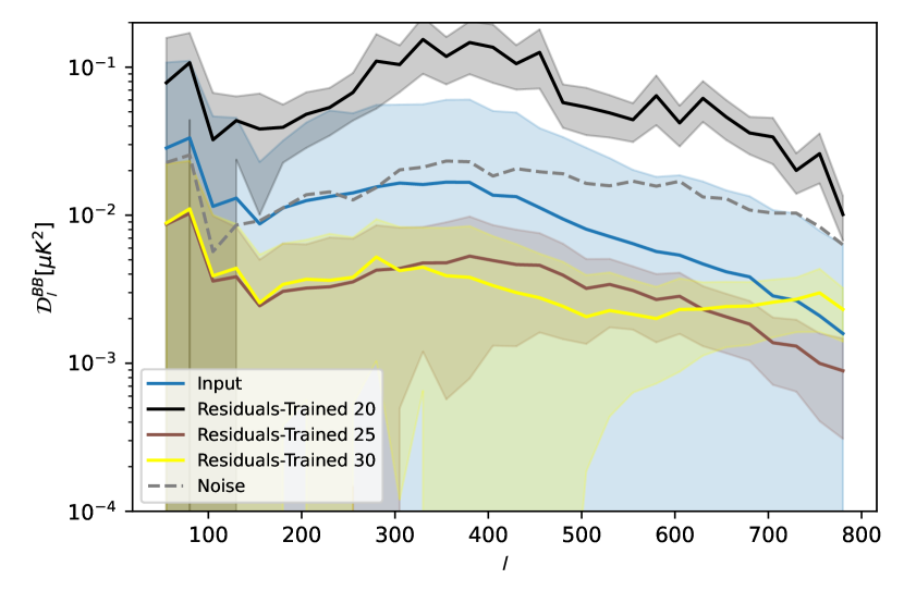
Figure 5: EE and BB residuals after training CENN at 20, 25 and 30 arcmin resolution and tested at 20 arcmin. Left panel: EE power spectra in the input simulations (blue line), residual patch average power spectra from CENN at 20 (black line), 25 (brown line) and 30 arcmin (yellow line). Right panel: the same but for the B-mode. In all cases, coloured areas shown the standard deviation of each bin, considered as the uncertainty of the model. Grey dashed line shows the higher instrumental noise levels seen by CENN.

Based on the results shown in the last case, we decided to train the network with patches at 20 arcmin resolution, testing not only this network but also the previous ones (30 and 25 arcmin) at this resolution. Figure 5 shows the EE and BB power spectra residuals, respectively, being the E-mode on the left panel and the B-mode on the right one in both cases. As in the previous cases, the comparison between both input and recovered signals is described in the Appendix A.

For the E-mode residuals, they are slightly higher at this training resolution with respect to the lower resolution cases, especially at middle and smaller scales ($l>400$). At larger scales, 20 and 30 arcmin residuals are similar while 25 arcmin ones are one order of magnitude higher than those cases. For the B-mode, residuals are about one order of magnitude above the CMB signal. However, although the noise levels are higher than the input signal, CENN recovers the B-mode for the other training cases with residuals one order of magnitude lower than the input. It seems that, training with higher resolution allows to obtain partially better results, at least until instrumental noise dominates the signal. In any case, based on these results, it seems that the network performs better when training with lower noise levels, although tested with higher ones.

4.4 Training at 5 arcmin and testing against d4s2 foreground model

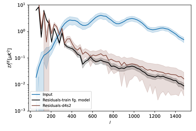
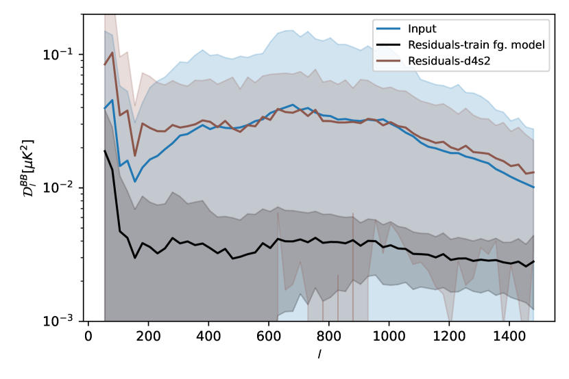
Figure 6: EE and BB residuals after training CENN at 5 arcmin resolution without noise. Left panel: EE power spectra in the input simulations (blue line), residual patch average power spectra from CENN for d6s1 (black line) and d4s2 (brown line) foreground models. Right panel: the same but for the B-mode. In all cases, coloured areas shown the standard deviation of each bin, considered as the uncertainty of the model.

Finally, we analyze the performance of CENN when the instrumental noise is negligible with respect to the CMB signal, which is likely the case with future CMB experiment. Moreover, we take the opportunity to assess CENN results when the foreground model is different from the one used in the network training. Therefore, we train CENN at 5 arcmin without noise, by producing two testing datasets: one with the same foreground model as in the training, and another with the d4s2 foreground model, in order to study the performance of the network recovering the E and B modes with a different microwave sky. After recovering $Q$ and $U$ CMB maps and applying NaMaster as in the previous cases, we plot in Figure 6 the EE and BB power spectra residuals, being the E-mode on the left panel and the B-mode on the right one.

Figure 6 shows the residuals in black and brown for the train and d4s2 foreground models, respectively. Without the instrumental noise, there is a clear improvement on the CENN results, both in angular resolution and residual levels. In the E-mode, there is a contamination of the foregrounds, over 1 $\mu K\hskip 1.0pt^{2}$, at large scales ($l<200$) in the residual patches. However, the performance improves while decreasing the angular scales, reaching residuals between $10^{-1}$ and $10^{-2}$ $\mu K\hskip 1.0pt^{2}$ for $l>500$. This behavior is similar for both foreground models.

For the B-mode, when testing with the same foreground model of the training dataset, CENN successfully recovers the B-mode signal with residuals of $7\times 10^{-3}$ $\mu K\hskip 1.0pt^{2}$. However, when testing with the different d4s2 foreground model, residuals increase to $3\times 10^{-2}$ $\mu K\hskip 1.0pt^{2}$, that is, CENN produced an artificial leackage with residual of the same order as the input signal.

5 Conclusions

In this work, we aim to use a new methodology based on neural networks called the cosmic microwave background extraction neural network (CENN), which showed a good performance recovering the total intensity CMB signal in Planck-like simulations in a previous work (Casas et al., 2022a). Actually, we re-train the neural network for recovering the E and B mode CMB polarization signal at sub-degree scales. CENN is simultaneously trained with 10000 realistic simulations of $Q$ and $U$ Planck maps consisting of 256$\times$256 pixel patches with a pixel size of 90 arcsec. Each simulation is formed by three patches at 100, 143 and 217 GHz with the CMB signal, thermal dust and synchrotron simulations from the PLA, injected PS and instrumental noise at Planck levels. The CMB signal at 143 GHz of each simulation is also used as a label for minimizing the loss function during training. All signals were smoothed with different Gaussian filters depending on the test, in order to improve the signal-to-noise-ratio on each pixel. The performance of the network is mainly analyzed by using the power spectra of the residual patch (input-output), while the comparisson between input and output signal is presented in the Appendix A.

Firstly, CENN was trained with 30 arcmin resolution patches. The E-mode become recovered with residuals between $10^{-1}$ and $10^{-2}$ $\mu K\hskip 1.0pt^{2}$ for the E-mode residuals, and a value between $2\times 10^{-3}$ $\mu K\hskip 1.0pt^{2}$ at $l<400$ and $5\times 10^{-4}$ $\mu K\hskip 1.0pt^{2}$ at $l>400$ for the B-mode ones.

Secondly, we compared the network trained with 25 arcmin resolution data with the previous one, both tested with 25 arcmin patches at the same position in the sky, obtaining similar residuals with respect to the previous case at large scales ($l<200$), while slighlty lower at $l>200$. On the other hand, the B-mode was slighly better recovered when trained with 25 arcmin patches. That is, the network is capable to learn smaller structures along the patch.

Thirdly, we compared the network trained with 20 arcmin resolution data with both 25 and 30 trained ones. In this case, the testing is done against 20 arcmin patches at the same location in the sky than in the previous cases. The residuals from the networks trained at lower resolution are generally lower than the input signal at about all scales for the E-mode, while the 20 arcmin network present residuals of one order of magnitude higher than the input signal for the B-mode. Although the network is capable to learn smaller structures when trained with higher resolution data, noise levels are crucial during the training procedure.

Finally, we trained the network with 5 arcmin resolution simulations without instrumental noise, but varying the foreground model. There is a clear improvement on the CENN results in terms of angular resolution and residual levels. In this case, we found that a different sky does not vary the performance of the neural network for the E-mode, obtaining similar residuals in both cases. However, we found a worse performance for the B-mode recovery, since the network introduced artifacts of the order of the input signal.

With these results about CMB recovery in polarization with neural networks we can firstly conclude that, fully-convolutional neural networks seem to be better for recovering structures at small scales than at middle and large scales. In all cases, but especially when we do not have any smoothing, the network have enough information in a small patch of the sky for always improving its performance when analyzing smaller scales. Previous works (Casas et al. 2022a, Casas et al. 2022b and Casas et al. 2023) present similar conclusions. As previously mentioned, future work extending the application of neural networks at all sky should be made to apply them in experiments such as LiteBIRD. The current CENN is better suited for experiments working with partial sky coverage, such as ACT, SPT, SO, POLARBEAR or the CMB-S4.

In any case, the evolution of the current CENN approach should be to use bigger patches. With the methodology used in this work, we cannot use bigger patches without having an E-to-B leakage. Moreover, with our patch sizes, we only can establish upper limits for the B-mode, at least at the resolutions used in this work. However, following other works which recover the CMB-signal, we must increase the patch size in order to solve this limitation, and we will be deal with in the future.

We also found that instrumental noise is relatively the more easily contaminant to segmentate from the CMB, at least whenever the noise levels are bellow the signal. In fact, as seen in Sect. 4.2 (training at 25 arcmin), CENN trained and applied to higher resolutions can be used as long as the noise level is reasonable with respect to the signal. When the noise becomes important as in Sect. 4.3 (training at 20 arcmin), it is better to train the network in good conditions, i.e. lower resolutions to get better results. This also affects to the large scale recovering, as seen in the comparison between 20, 25 and 30 arcmin training. When training with lower levels of instrumental noise, although tested with higher contamination, the recovering is more accurate than training at the same conditions than during the testing when instrumental noise dominate the signal. This fact could be relevant for studying a future constrain of the tensor-to-scalar ratio with neural networks.

Based on these results, it seems to be better to train a neural network without noise, although being included in the patches of the testing set. This seems reasonable since we think a neural network might get ”confused” by the noise presence while optimizing its weights. In any case, this should be tested in future works in order to start using neural networks for systhematics cleaning, which could be extremely relevant for future CMB experiments searching for the primordial B-mode signal.

Another relevant aspect is that, as expected, B-mode recovery is sensitive to the use of a different foreground model. In order to mitigate this limitation, what can be done is to have various networks trained with different foreground models before their application to the data and analyze and compare the outputs from the different networks, for example, in terms of power spectra.

Appendix A Recovered power spectrum

This appendix shows the comparison between both input and recovered EE and BB power spectra for the previously described 30, 25, 20 and 5 arcmin resolution testing datasets.

Firstly, Fig 7 show the testing at 30 arcmin, where the E-mode is recovered with high accuracy, showing a difference between the input simulations (blue line) and the recovered signal (red line) of about 0.1 $\pm$ 0.3 $\mu K\hskip 1.0pt^{2}$. On the other hand, the B-mode is similarly recovered at all scales for the training resolution, with a difference of about 0.002 $\pm$ 0.02 $\mu K\hskip 1.0pt^{2}$.

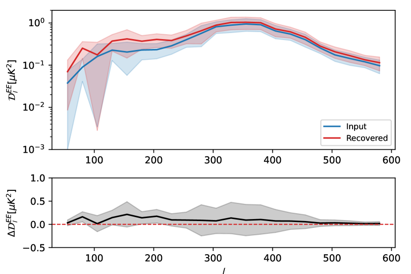
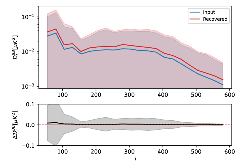
Figure 7: EE and BB power spectra recovery after training and testing CENN at 30 arcmin resolution. Left top panel: EE power spectra in the input simulations (blue line) and patch average output power spectra from CENN at 30 arcmin red line. Left bottom panel: Difference between input and recovered EE power spectra at 30 arcmin (black line). Right panel: the same but for the B-mode. In all cases, coloured areas shown the standard deviation of each bin, considered as the uncertainty of the model. Red dashed lines in bottom sub-panels represent the ideal case.

Figure 8 shows the comparison between the 25 and 30 trained networks, both tested at 25 arcmin. The E-mode is also recovered with higher accuracy at the training resolution of 25 arcmin, with a difference between the input simulations (blue line) and the recovered signal (red line) of less than 0.1 $\pm$ 0.5 $\mu K\hskip 1.0pt^{2}$, with a difference of 0.3 $\mu K\hskip 1.0pt^{2}$ with respect of training CENN at 30 arcmin resolution. The recovering of the B-mode is also improved when training at lower resolution by a value between 0.005 and 0.01 $\mu K\hskip 1.0pt^{2}$, with similar uncertainties in both cases.

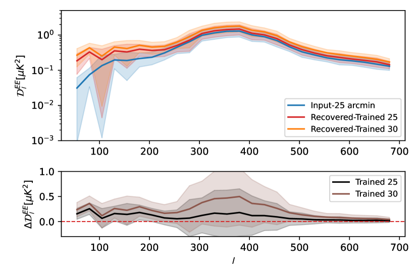
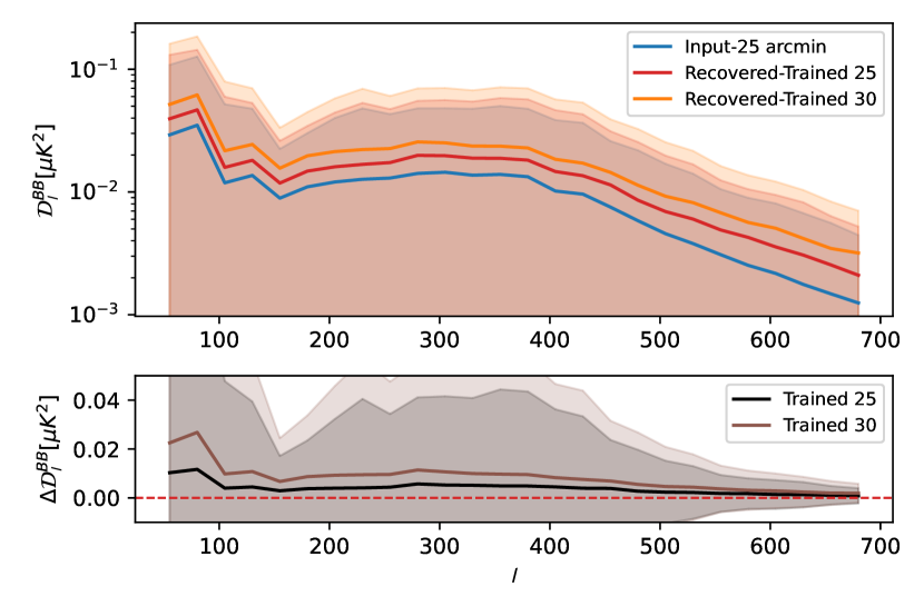
Figure 8: EE and BB power spectra recovery after training CENN at 25 and 30 arcmin resolution and tested at 25 arcmin. Left top panel: EE power spectra in the input simulations (blue line), patch average output power spectra from CENN trained at 25 (red line) and 30 arcmin (orange line). Left bottom panel: Difference between input and recovered EE power spectra from CENN trained at 25 arcmin (black line) and 30 arcmin (brown line). Right panel: the same but for the B-mode. In all cases, coloured areas shown the standard deviation of each bin, considered as the uncertainty of the model. Red dashed lines in bottom sub-panels represent the ideal case.

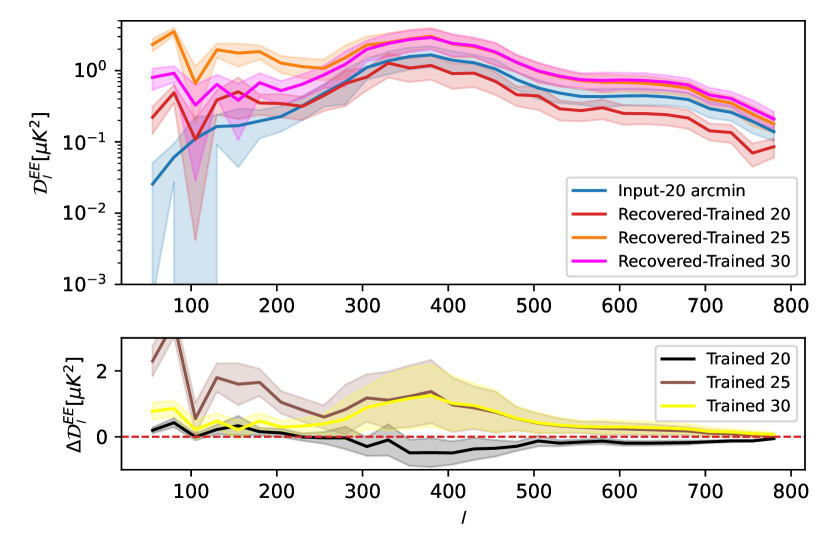
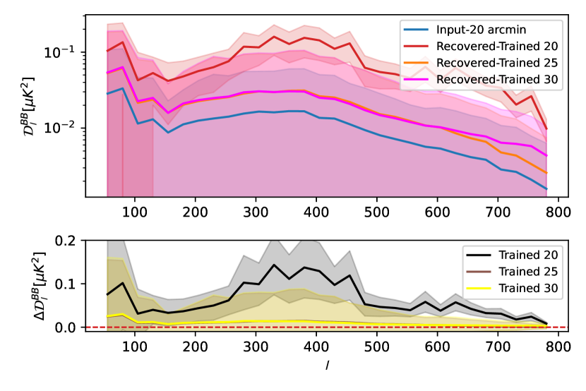
Figure 9: EE and BB power spectra recovery after training CENN at 20, 25 and 30 arcmin resolution and tested at 20 arcmin. Left top panel: EE power spectra in the input simulations (blue line), patch average output power spectra from CENN trained at 20 (red line), 25 (orange line) and 30 arcmin (magenta line). Left bottom panel: Difference between input and recovered EE power spectra from CENN trained at 20 (black line), 25 (brown line) and 30 arcmin (yellow line). Right panel: the same but for the B-mode. In all cases, coloured areas shown the standard deviation of each bin, considered as the uncertainty of the model. Red dashed lines in bottom sub-panels represent the ideal case.

Figure 9 shows the comparison between the 20, 25 and 30 trained networks, both tested at 20 arcmin. The E-mode is better recovered with respect to the 25 and 30 arcmin training, with a difference between the input simulations (blue line) and the recovered signal (red line) of less than 0.4 $\pm$ 0.3$\hskip 1.0pt\mu K\hskip 1.0pt^{2}$, a 0.7 $\mu K\hskip 1.0pt^{2}$ better recovering than in the 30 arcmin training at middle scales, and similarly for the 25 arcmin training. At large scales, results are similar with respect the 30 arcmin training but worse than the 25 arcmin case, with a difference of more than 2$\hskip 1.0pt\mu K\hskip 1.0pt^{2}$. Finally, at small scales, when training at 20 arcmin resolution we obtain a 0.1$\hskip 1.0pt\mu K\hskip 1.0pt^{2}$ more accurate signal than the other two cases. However, the recovering of the B-mode is worse than in the previous cases, due to an absolute error value between 0.05 and 0.1 $\mu K\hskip 1.0pt^{2}$ for both 25 and 30 arcmin trainings. The difference between input and recovered signal is between 0.04 and 0.9 $\mu K\hskip 1.0pt^{2}$ lower.

Finally, Fig. 10 shows the performance of CENN trained and tested at 5 arcmin resolution patches without noise. The E-mode is recovered with a difference less than 2 $\mu K\hskip 1.0pt^{2}$ for multipoles $l>200$. In fact, for middle and small scales, the difference between the E-mode in the input simulations (blue line) and the recovered signal by the neural network (red and orange lines for the train and d4s2 foreground models, respectively), is similar, with a value between 1 $\pm$ 1 $\mu K\hskip 1.0pt^{2}$ and 0.5 $\pm$ 1 $\mu K\hskip 1.0pt^{2}$. Furthermore, at even small scales ($l$ ¿ 1200) the recovering is almost perfect. On the contrary, at large scales ($l$ ¡ 200), the performance is similar than the previous cases, having a mislead recovery with a difference higher than 2 $\mu K\hskip 1.0pt^{2}$, although the performance is similar for both foreground models. On the other hand, the B-mode is recovered with high accuracy when testing with the same foreground model used for training the network, with an upper limit difference between input and recovered one of about 0.01 $\mu K\hskip 1.0pt^{2}$. For the d4s2 foreground model, the performance is similar but a bit worse, with an upper limit difference between input and recovered of about 0.04 $\mu K\hskip 1.0pt^{2}$. At large scales ($l<200$), the B-mode is recovered with worse accuracy for the d4s2 model than for the training one, with a difference of 0.12 $\mu K\hskip 1.0pt^{2}$ in the d4s2 case and a difference of 0.02 $\mu K\hskip 1.0pt^{2}$ in the training one.

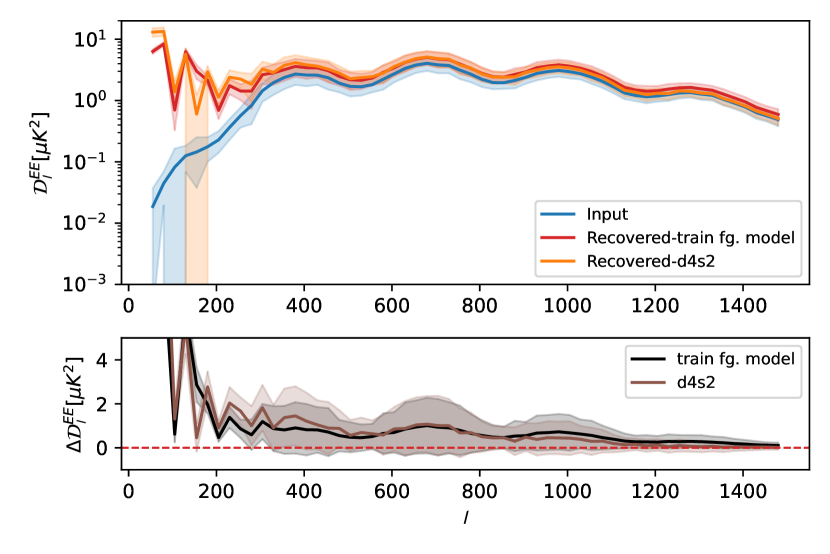
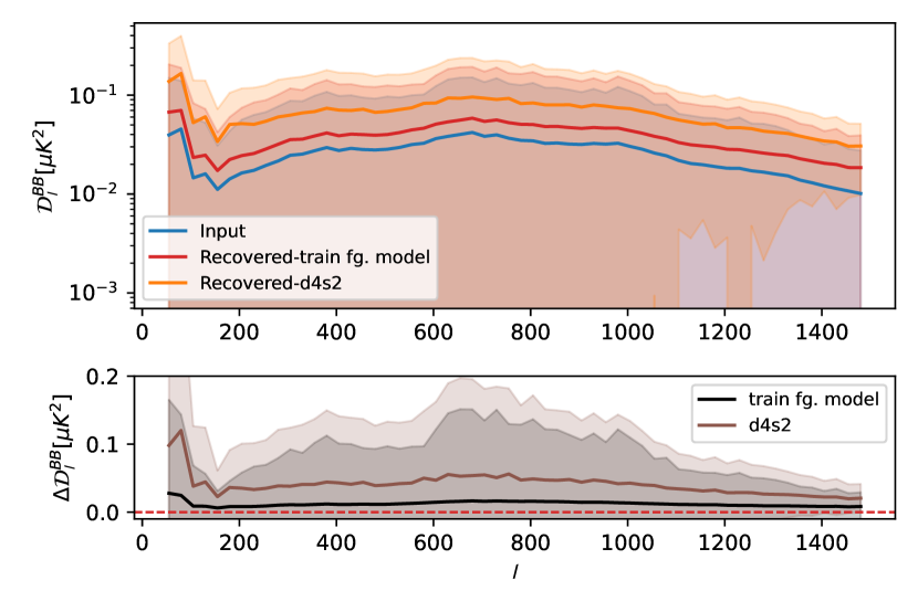
Figure 10: EE and BB power spectra recovery after training CENN at 5 arcmin resolution without noise. Left top panel: EE power spectra in the input simulations (blue line), patch average output power spectra from CENN training foreground model (red line) and d4s2 (orange line) foreground models. Left bottom panel: Difference between input and recovered EE power spectra from CENN for the training (black line) and d4s2 (brown line) foreground models. Right panel: the same but for the B-mode. In all cases, coloured areas shown the standard deviation of each bin, considered as the uncertainty of the model. Red dashed lines in bottom sub-panels represent the ideal case.

References

- Abazajian et al. (2022) Abazajian, K., Abdulghafour, A., Addison, G. E., et al. 2022, arXiv e-prints, arXiv:2203.08024
- Baccigalupi (2003) Baccigalupi, C. 2003, New A Rev., 47, 1127
- Baumann (2009) Baumann, D. 2009, arXiv e-prints, arXiv:0907.5424
- Bicep/Keck Collaboration et al. (2021) Bicep/Keck Collaboration, Ade, P. A. R., Ahmed, Z., et al. 2021, Phys. Rev. Lett., 127, 151301
- Bonavera et al. (2017) Bonavera, L., González-Nuevo, J., Argüeso, F., & Toffolatti, L. 2017, MNRAS, 469, 2401
- Bonavera et al. (2021) Bonavera, L., Suarez Gomez, S. L., González-Nuevo, J., et al. 2021, A&A, 648, A50
- Casas et al. (2022a) Casas, J. M., Bonavera, L., González-Nuevo, J., et al. 2022a, A&A, 666, A89
- Casas et al. (2023) Casas, J. M., Bonavera, L., González-Nuevo, J., et al. 2023, A&A, 670, A76
- Casas et al. (2022b) Casas, J. M., González-Nuevo, J., Bonavera, L., et al. 2022b, A&A, 658, A110
- Chluba et al. (2017) Chluba, J., Hill, J. C., & Abitbol, M. H. 2017, MNRAS, 472, 1195
- Chollet (2015) Chollet, F. 2015, Keras, https://github.com/fchollet/keras
- Delabrouille et al. (2009) Delabrouille, J., Cardoso, J. F., Le Jeune, M., et al. 2009, A&A, 493, 835
- Delabrouille et al. (2003) Delabrouille, J., Cardoso, J. F., & Patanchon, G. 2003, MNRAS, 346, 1089
- Eriksen et al. (2008) Eriksen, H. K., Jewell, J. B., Dickinson, C., et al. 2008, ApJ, 676, 10
- Farsian et al. (2020) Farsian, F., Krachmalnicoff, N., & Baccigalupi, C. 2020, J. Cosmology Astropart. Phys., 2020, 017
- Fernández-Cobos et al. (2012) Fernández-Cobos, R., Vielva, P., Barreiro, R. B., & Martínez-González, E. 2012, MNRAS, 420, 2162
- Fuskeland et al. (2021) Fuskeland, U., Andersen, K. J., Aurlien, R., et al. 2021, A&A, 646, A69
- Fuskeland et al. (2023) Fuskeland, U., Aumont, J., Aurlien, R., et al. 2023, arXiv e-prints, arXiv:2302.05228
- González-Nuevo et al. (2005) González-Nuevo, J., Toffolatti, L., & Argüeso, F. 2005, ApJ, 621, 1
- Goodfellow (2010) Goodfellow, I. J. 2010, Technical Report: Multidimensional, Downsampled Convolution for Autoencoders, Tech. rep., Université de Montréal
- Goodfellow et al. (2016) Goodfellow, I. J., Bengio, Y., & Courville, A. 2016, Deep Learning (Cambridge, MA, USA: MIT Press), http://www.deeplearningbook.org
- Górski et al. (2005) Górski, K. M., Hivon, E., Banday, A. J., et al. 2005, ApJ, 622, 759
- Guth (1981) Guth, A. H. 1981, Phys. Rev. D, 23, 347
- Hensley & Draine (2021) Hensley, B. S. & Draine, B. T. 2021, ApJ, 906, 73
- Hu & White (1997) Hu, W. & White, M. 1997, New A, 2, 323
- Hunter (2007) Hunter, J. D. 2007, Computing In Science & Engineering, 9, 90
- Jeffrey et al. (2022) Jeffrey, N., Boulanger, F., Wandelt, B. D., et al. 2022, MNRAS, 510, L1
- Kamionkowski et al. (1997) Kamionkowski, M., Kosowsky, A., & Stebbins, A. 1997, Phys. Rev. Lett., 78, 2058
- Krachmalnicoff et al. (2016) Krachmalnicoff, N., Baccigalupi, C., Aumont, J., Bersanelli, M., & Mennella, A. 2016, A&A, 588, A65
- Krachmalnicoff et al. (2018) Krachmalnicoff, N., Carretti, E., Baccigalupi, C., et al. 2018, A&A, 618, A166
- Krachmalnicoff & Puglisi (2021) Krachmalnicoff, N. & Puglisi, G. 2021, ApJ, 911, 42
- Krachmalnicoff & Tomasi (2019) Krachmalnicoff, N. & Tomasi, M. 2019, A&A, 628, A129
- Leach et al. (2008) Leach, S. M., Cardoso, J. F., Baccigalupi, C., et al. 2008, A&A, 491, 597
- Linde (1982) Linde, A. D. 1982, Physics Letters B, 108, 389
- LiteBIRD Collaboration et al. (2022) LiteBIRD Collaboration, Allys, E., Arnold, K., et al. 2022, arXiv e-prints, arXiv:2202.02773
- Oliphant (2006) Oliphant, T. 2006, NumPy: A guide to NumPy, USA: Trelgol Publishing, [Online; accessed ¡today¿]
- Perraudin et al. (2019) Perraudin, N., Defferrard, M., Kacprzak, T., & Sgier, R. 2019, Astronomy and Computing, 27, 130
- Petroff et al. (2020) Petroff, M. A., Addison, G. E., Bennett, C. L., & Weiland, J. L. 2020, The Astrophysical Journal, 903, 104
- Planck Collaboration et al. (2018) Planck Collaboration, Akrami, Y., Arroja, F., et al. 2018, arXiv e-prints, arXiv:1807.06205
- Planck Collaboration V (2020) Planck Collaboration V. 2020, A&A, 641, A5
- Puglisi & Bai (2020) Puglisi, G. & Bai, X. 2020, ApJ, 905, 143
- Puglisi et al. (2018) Puglisi, G., Galluzzi, V., Bonavera, L., et al. 2018, ApJ, 858, 85
- Puglisi et al. (2022) Puglisi, G., Mihaylov, G., Panopoulou, G. V., et al. 2022, MNRAS, 511, 2052
- Remazeilles et al. (2011) Remazeilles, M., Delabrouille, J., & Cardoso, J.-F. 2011, MNRAS, 418, 467
- Remazeilles et al. (2021) Remazeilles, M., Rotti, A., & Chluba, J. 2021, MNRAS, 503, 2478
- Rumelhart et al. (1986) Rumelhart, D. E., Hinton, G. E., & Williams, R. J. 1986, Nature, 323, 533
- Stompor et al. (2009) Stompor, R., Leach, S., Stivoli, F., & Baccigalupi, C. 2009, MNRAS, 392, 216
- Thorne et al. (2017) Thorne, B., Dunkley, J., Alonso, D., & Næss, S. 2017, MNRAS, 469, 2821
- Tucci & Toffolatti (2012) Tucci, M. & Toffolatti, L. 2012, Advances in Astronomy, 2012, 624987
- Tucci et al. (2011) Tucci, M., Toffolatti, L., de Zotti, G., & Martínez-González, E. 2011, A&A, 533, A57
- Vacher et al. (2022) Vacher, L., Aumont, J., Montier, L., et al. 2022, A&A, 660, A111
- Vansyngel et al. (2017) Vansyngel, F., Boulanger, F., Ghosh, T., et al. 2017, A&A, 603, A62
- Wang et al. (2022) Wang, G.-J., Shi, H.-L., Yan, Y.-P., et al. 2022, ApJS, 260, 13
- Wei et al. (2021) Wei, X.-S., Song, Y.-Z., Mac Aodha, O., et al. 2021, IEEE Transactions on Pattern Analysis and Machine Intelligence
- Wes McKinney (2010) Wes McKinney. 2010, in Proceedings of the 9th Python in Science Conference, ed. Stéfan van der Walt & Jarrod Millman, 56 – 61
- Yan et al. (2023) Yan, Y.-P., Wang, G.-J., Li, S.-Y., & Xia, J.-Q. 2023, arXiv e-prints, arXiv:2302.13572
- Zaldarriaga & Seljak (1997) Zaldarriaga, M. & Seljak, U. 1997, Phys. Rev. D, 55, 1830
- Zonca et al. (2019) Zonca, A., Singer, L. P., Lenz, D., et al. 2019, Journal of Open Source Software, 4, 1298
- Zonca et al. (2021) Zonca, A., Thorne, B., Krachmalnicoff, N., & Borrill, J. 2021, The Journal of Open Source Software, 6, 3783