Boundedness of solutions of nonautonomous
degenerate logistic equations

Abstract. In this work we analyze the boundedness properties of the solutions of a nonautonomous parabolic degenerate logistic equation in a bounded domain. The equation is degenerate in the sense that the logistic nonlinearity vanishes in a moving region, $K(t)$, inside the domain. The boundedness character of the solutions depends not only on, roughly speaking, the first eigenvalue of the Laplace operator in $K(t)$ but also on the way this moving set evolves inside the domain and in particular on the speed at which it moves.

Keywords: nonautonomous; evolution equation; degenerate logistic; boundedness;

1 Introduction

In this work we study the behavior of the solutions of a nonautonomous evolution problem of the type

$$\left\{\begin{array}[]{lr}u_{t}-\Delta u=\lambda u-n(t,x)|u|^{\rho-1}u,&x\in\Omega,\;t>t_{0},\\ u=0,&x\in\partial\Omega,\;t>t_{0},\\ u(t_{0},x)=u_{0}(x)\geq 0,&x\in\Omega,\end{array}\right.$$ (1.1)

where $\Omega$ is a bounded and smooth domain in $\mathbb{R}^{N}$, for some positive integer $N$, $\rho>1,t_{0},\lambda\in\mathbb{R}$, $n\in L^{\infty}(\mathbb{R}\times\Omega)$ with $n\geq 0$ and $0\leq u_{0}\in L^{q}(\Omega)$ where $1<q\leq\infty$ will be chosen appropriately large enough. We consider Dirichlet boundary conditions but the analysis could be developed for other boundary conditions.

The set where the function $n(t,\cdot)$ vanishes is denoted by $K(t)$, that is,

$$K(t):=\left\{x\in\overline{\Omega}:n(t,x)=0\right\},\;\;t\in\mathbb{R}.$$ (1.2)

that we assume is compact for every $t\in\mathbb{R}$, probably empty for some times or even the entire domain for other intervals of time.

Notice that we are not assuming any special structure of the function $n(t,x)$. We are not restricting ourselves to the periodic case, that is $n(t+T,x)=n(t,x)$ for certain $T>0$ or even to quasiperiodic or almost periodic cases. These are relevant and very interesting cases, but we are aiming to cover general nonatuonomous situation, including these ones.

From a population dynamics interpretation, see [cantrellcosner], equation (1.1) represents the evolution of the density of certain population, $u(x,t)$, in certain habitat given by the domain $\Omega$. The species diffuses inside the domain and the fact that the boundary condition are homogeneous Dirichlet represents that the exterior of the habitat is very hostile for the species and no individual of the species survives outside the habitat. The term $\lambda u$ represent the natural growth rate of the species, that we assume to be constant and the term $-n(t,x)|u|^{\rho-1}u$ represents a logistic term that opposes to the natural growth of the population. If for instance $n(t,x)\geq\beta>0$ throughout the domain, we have that if $u$ is large then the term $\lambda u-n(t,x)|u|^{\rho-1}u<0$ and the population decreases so that we do not expect large values of $u$.

The case where $n(t,x)\equiv n(x)$, so that the equation becomes autonomous, that is

$$\left\{\begin{array}[]{lr}u_{t}-\Delta u=\lambda u-n(x)|u|^{\rho-1}u,&x\in\Omega,\;t>t_{0},\\ u=0,&x\in\partial\Omega,\;t>t_{0},\\ u(t_{0},x)=u_{0}(x)\geq 0,&x\in\Omega,\end{array}\right.$$ (1.3)

has been addressed in the literature when $n(x)\geq\beta>0$ throughout the domain ,see for instance [cantrellcosner, murray], and also when $n(\cdot)$ vanishes at some region $K_{0}$ of the domain, that is,

$$K_{0}=\{x\in\bar{\Omega}:\,n(x)=0\},$$

see [AnibalArrietaPardo, Julian2] and references therein. Following again the population dynamics interpretation, the set $K_{0}$ represents a gifted location where the species is able to grow whereas $\Omega\setminus K_{0}$ represents a location where the species encounters hardships such as predators, harsh terrain, low resources or intraspecies competition. We refer to $K_{0}$ as a “sanctuary” for the species. Then, by means of the diffusion, part of the growth attained in $K_{0}$ is migrated outside $K_{0}$ where the hard conditions threaten the growth of the species. It is natural to see that the size of $K_{0}$ and the strength of the intrinsic growth rate $\lambda$ will play a key role determining whether the species keeps growing forever or remains bounded.

Also, in many places in the literature it is considered the case where the function $n(x)$ is regular (at least continuous) and $K_{0}$ is the closure of a regular open set $\Omega_{0}$, that is $K_{0}=\bar{\Omega}_{0}$, see for instance [Julian2] and references therein. With these conditions, the asymptotic behavior of solutions of (1.1) has been studied. Denoting by $\lambda_{1}^{\Omega}$ the first eigenvalue of the Laplace operator with homogeneous Dirichlet boundary conditions on $\Omega$, it is known that if $\lambda<\lambda_{1}^{\Omega}$ then $0$ is the unique equilibrium which is globally asymptotically stable and therefore all solutions approach $0$ when $t\rightarrow\infty$. If $\lambda>\lambda_{1}^{\Omega}$ then $0$ becomes unstable, and solutions tend to grow away from it. As a matter of fact, if $\lambda_{1}^{\Omega}<\lambda<\lambda_{1}^{\Omega_{0}}$ then solutions tend to the unique globally asymptotically stable positive equilibrium $u_{eq}$. On the other hand, if $\lambda>\lambda_{1}^{\Omega_{0}}$ then solutions have been shown to grow and become unbounded as $t\rightarrow\infty$ only on $K_{0}$ but they remain bounded outside $K_{0}$, which will be referred to as “grow up”. We refer to [Julian2] for a rather complete study of this case. Hence, these results can be summarised as follows:

$$\left\{\begin{array}[]{ll}\mbox{If }\lambda<\lambda_{1}^{\Omega}&\Rightarrow u\rightarrow 0,\\ \mbox{If }\lambda_{1}^{\Omega}<\lambda<\lambda_{1}^{\Omega_{0}}&\Rightarrow u\rightarrow u_{eq},\\ \mbox{If }\lambda_{1}^{\Omega_{0}}<\lambda&\Rightarrow u(x)\rightarrow\infty,\quad x\in\Omega_{0}.\end{array}\right.$$ (1.4)

An extension of (1.4) to the case where $K_{0}$ is only assumed to be compact without any further regularity assumptions was studied in [AnibalArrietaPardo]. In [AnibalArrietaPardo], the role of $\lambda_{1}^{\Omega_{0}}$ is substituted by $\lambda_{0}(K_{0})$, the characteristic value of the set $K_{0}$, which is defined as follows: consider $\{\Omega_{\delta}\}_{0<\delta\leq\delta_{0}}$ a nested decreasing family of smooth open sets satisfyng $K_{0}=\bigcap_{0<\delta\leq\delta_{0}}\Omega_{\delta}$ and define

$$\lambda_{0}(K_{0}):=\lim\limits_{\delta\rightarrow 0^{+}}\lambda_{1}^{\Omega_{\delta}}.$$

Notice that $\lambda_{0}(K_{0})$ can be $+\infty$ if $K_{0}$ is “small”, for example, when $K_{0}$ is a point in $\Omega$. If $K_{0}$ is regular, that is, $K_{0}=\bar{\Omega}_{0}$ for some regular open set $\Omega_{0}$, then it is possible to show that $\lambda_{0}(K_{0})=\lambda_{1}^{\Omega_{0}}$. In [AnibalArrietaPardo] authors show that if $\lambda<\lambda_{0}(K_{0})$ then all solutions are bounded and if $\lambda\geq\lambda_{0}(K_{0})$ solutions grow up without bound as time goes to $+\infty$.

We summarize this results in Figure 1.

Figure 1: A representation of the cases shown in (1.4).

Therefore, for the autonomous case, the key factor that decides whether the solutions are bounded or unbounded is the relation between $\lambda$ and $\lambda_{0}(K_{0})$: if $\lambda<\lambda_{0}(K_{0})$ solutions remain bounded whereas if $\lambda\geq\lambda_{0}(K_{0})$ solutions become unbounded as $t\rightarrow\infty$. Moreover, in general terms observe that the smaller $K_{0}$ is, the larger $\lambda_{0}(K_{0})$ is. Therefore, smaller $K_{0}$ imply that it is more likely to have $\lambda<\lambda_{0}(K_{0})$ and thus, boundedness. And viceversa, the larger the set $K_{0}$, the smaller $\lambda_{0}(K_{0})$ is and the more likely that solutions will grow.

In the nonautonomous case, that is problem (1.1), the situation is not so simple and, as we will see in this work, the relation between $\lambda$ and $\lambda_{0}(K(t))$ will not be enough to decide the boundedness or unboundedness of the solutions. Note that $\lambda_{0}(K(t))$ is time dependent and we may not have $\lambda<\lambda_{0}(K(t))$ for all $t$ or $\lambda>\lambda_{0}(K(t))$ for all $t$. Moreover, as we will see below, even in the case $\lambda>\lambda_{0}(K(t))$ for all $t$ we may not have grow–up and if $\lambda<\lambda_{0}(K(t))$ may not have boundedness. Therefore, the characterization of boundedness or unboundedness of solutions for the nonautonomous case is not so straightforward as in the case of autonomous problems. As a matter of fact, many interesting questions appear in the nonautonomous case. Does the geometry of the sets $K(t)$ determine the boundedness character of the solutions? Is the velocity at which the sets $K(t)$ evolve important to decide the boundedness? We will see that both the geometry and velocity of the sets $K(t)$ are important factors to take into consideration to decide the boundeness character of the solutions.

To conclude this introduction, we would like to mention that the results of the present article are a necessary first step to analyze the asymptotic behavior of the solutions of these nonautonomous degenerate logistic equations. In the cases where boundedness is obtained we should question ourselves about the existence of attractors, their fine structure and behavior. In the case of unboundedness, we should try to understand how and where the solution becomes unbounded as $t\to+\infty$. Most likely, the set where the solution becomes unbounded (the “grow-up set”) will be a moving set. These issues will be treated in future publications.

With respect to boundedness, let us mention that there are several interesting works in the literature addressing the general problem of the asymptotic behavior of solutions for nonautonomous problems, analyzing the existence of different kind of asymptotic sets which respond to different concepts of attraction like pullback, forwards, uniform attractors and which describe the behavior of the systems for large times. Without being exhaustive we would like to mention the monograph [Carvalho2013] and references therein for a nice and rather complete reference in this respect. We also mention the works [anibal2007, tesisAVL] where the authors construct complete trajectores for both autonomous and nonoautonomous parabolic evolution equations, which bound the asymptotic dynamics of the evolution processes. The works [langa2007, langa2002pullback] are also relevant in this respect.

Moreover, there are some other interesting works that deal with the periodic case, that is $n(t+T,x)=n(t,x)$ for all $t\in\mathbb{R}$, $x\in\Omega$ and obtain results on existence of periodic solutions under different hypotheses. In particular, if $K(t)$ is static, that is $K(t)\equiv K_{0}$, existence results of periodic solutions (and therefore, boundedness) were already proven in [Julian3]. Very recently in [Aleja], authors generalise results in [Julian3] and characterize the existence of periodic solutions without imposing $K(t)$ being static. In particular, authors prove a very interesting result where they give an if and only if characterization for the existence of periodic solutions in terms of the behavior of certain nontrivial periodic parabolic eigenvalue problems. This interesting technique is specific for periodic situations and do not apply directly to our most general nonautonomous scenario. See also [DancerHess, Julian4] for some related results on periodic parabolic problems.

With respect to unboundedness, we should try to understand how and where the solution becomes unbounded as $t\to+\infty$. Most likely, the set where the solution becomes unbounded (the “grow-up set”) will be a moving set but to identify it and study the asympotic properties of these systems requires further analysis. These issues will be treated in future publications.

We describe now the contents of the paper.

In Section 2 we include some preliminary results like local and global existence of mild solutions and regularity of solutions. We also recall comparison results with respect to initial data, nonlinearity and domain.

In Section LABEL:Section-data-independence we include an important result that says that the boundedness or unboundedness character of the solution evaluated at a particular point $x\in\Omega$ does not depend on initial time or the initial data $u_{0}$ (as long as $u_{0}\geq 0$ and $u_{0}\not\equiv 0$). Therefore if for one particular nontrivial initial data $u_{0}$ and initial time $\tau_{0}$ its solution is asymptotically bounded at $x$, that is $\limsup_{t\to+\infty}u(t,x)<+\infty$, then for any other nontrivial initial data and initial time we also have that the limsup is finite. This result is based on comparison results, regularity and the parabolic Hopf Lemma.

In Section LABEL:Section-general-result we prove a first result that applies to many situations since we do not impose many restrictions on the configuration of the family of sets $K(t)$. Roughly speaking, the idea is the following: if we assume a nondegeneracy condition of the function $n(t,x)$ (see Assmption (N)) and consider the upper and lower limit of the family of sets $K(t)$, that is $\overline{\bigcup\limits_{t\geq\tau_{0}}K(t)}$, $\bigcap\limits_{t\geq\tau_{0}}K(t)$, then if $\lambda<\lambda_{0}(\overline{\bigcup\limits_{t\geq\tau_{0}}K(t)})$ we have boundedness of solutions, while if $\lambda>\lambda_{0}(\bigcap\limits_{t\geq\tau_{0}}K(t))$ we have unboundeness of solutions, see Proposition LABEL:prop-boundedness-general and Corollary LABEL:cor-boundedness-general. We also include in this section some relevant examples that allow us to clarify the meaning of these sets.

In Section LABEL:secBound we address situations where the rather general condition of the previous section does not apply and in particular we have $\lambda_{0}(\overline{\bigcup\limits_{t\geq\tau_{0}}K(t)})<\lambda<\lambda_{0}(\bigcap\limits_{t\geq\tau_{0}}K(t))$.

A first important case covered in this section says, roughly speaking, that if $n(t,x)\geq\nu_{0}>0$ (and therefore $K(t)=\emptyset$) for a sequence of time intervals $I_{1}$, $I_{2}$, etc. with the condition that the length of each of them is bounded below by a quantity $\eta>0$ and the distance between two consecutive intervals is no larger than a quantity $\Xi$, then, independently of the value of $\lambda$, all solutions are bounded, see Proposition LABEL:PropInter. That is, the effective presence of the logistic term in the entire domain and at the intervals of time $I_{1}$, $I_{2}$, etc. which do not degenerate and they are not too far away from the next, guarantees the boundedness of solutions.

Next, we show that, roughly speaking and oversimplifying the conditions, if $\lambda<\lambda_{0}(K(t))$ for all $t$ large enough then we have boundedness of solutions. The precise statement is contained in Theorem LABEL:TeoAcot1. A very important example where this theorem applies is contained in Remark LABEL:RecondAcotLambdaSmall where a fix set $K_{0}$ is considered and we assume that $K(t)$ consists in moving (translation by a curve $\gamma(t)$ and a rotation) the set $K_{0}$ inside $\Omega$ see Figure 2.

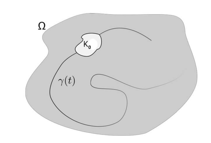
Figure 2: Domain $\Omega$ and a continuously moving $K(t)$.

In this section we also consider the case where the set $K(t)$ allows jumps. A good example of this situation is when we consider the existence of a sequence $t_{0}<t_{1}<t_{2}<\ldots$, such that $K(t)=K_{0}$ for $t\in(t_{2k},t_{2k+1})$ and $K(t)=K_{1}$ for $t\in(t_{2k+1},t_{2k+2})$. Hence, the set $K(t)$ jumps from $K_{0}$ to $K_{1}$ and back to $K_{0}$ at certain instants of time. We show that if $K_{0}\cap K_{1}=\emptyset$ then independently of the value of $\lambda$ all solutions are bounded.

Finally, in Section LABEL:secUnbound we analyze conditions under which solutions become unbounded. In view of the results of Theorem LABEL:TeoAcot1 where boundedness is established for, roughly speaking, $\lambda<\lambda_{0}(K(t))$ for all $t$, it seems natural to ask whether for $\lambda>\lambda_{0}(K(t))$ for all $t$, we have unboundedness of solutions. This is actually true if the equation is autonomous, see [AnibalArrietaPardo] for instance. But notice that Theorem LABEL:TeoAcot and the example where $K(t)$ jumps between two sets $K_{0}$ and $K_{1}$ with $K_{0}\cap K_{1}=\emptyset$ and $\lambda$ arbitrary and in particular we could consider $\lambda>\lambda_{0}(K_{0}),\lambda_{0}(K_{1})$, means that this is not true in a general setting. As a matter of fact, we will be able to show that if, roughly speaking, $K(t)$ moves “slowly” and $\lambda>\lambda_{0}(K(t))$ for all $t$, then we have unboundedness of solutions. The precise statement of this result is Theorem LABEL:TeoUnbounded. We also analyze a situation where the condition $\lambda>\lambda_{0}(K(t))$ for all $t$ can be weakened, see Proposition LABEL:PropUnbound.

Acknowledgements. José M. Arrieta is partially supported by grants PID2019-103860GB-I00, PID2022-137074NB-I00 and CEX2019-000904-S “Severo Ochoa Programme for Centres of Excellence in R&D” the three of them from MICINN, Spain. Also by “Grupo de Investigación 920894 - CADEDIF”, UCM, Spain. Marcos Molina-Rodríguez is partially supported by the predoctoral appointment BES-2013-066013, grant PID2019-103860GB-I00 both by MICINN, Spain and by “Grupo de Investigación 920894 - CADEDIF”, UCM, Spain. Lucas A. Santos is partially supported by the Coordenação de Aperfeiçoamento de Pessoal de Nível Superior – Brasil (CAPES) – Finance Code 001”

2 Preliminaries

Equation (1.1) is a particular case of a more general class of parabolic nonautonomous equations:

$$\left\{\begin{array}[]{lr}u_{t}-\Delta u=f(t,x,u),&x\in\Omega,\;t>t_{0},\\ u=0,&x\in\partial\Omega,\;t>t_{0},\\ u(t_{0},x)=u_{0}(x),&x\in\Omega,\end{array}\right.$$ (2.1)

where $f:\mathbb{R}\times\Omega\times\mathbb{R}\rightarrow\mathbb{R}$ satisfies

$$\begin{array}[]{l}\left|f(t,x,u)-f(t,x,v)\right|\leq C\left|u-v\right|\left(\left|u\right|^{\rho-1}+\left|v\right|^{\rho-1}+1\right),\;\mbox{ for }u,v\in\mathbb{R},\,\,t\geq t_{0},\end{array}$$ (2.2)

for certain constant $C$ uniformly for $t\geq t_{0}$ on bounded sets and $x\in\Omega$. Observe that if $n\in L^{\infty}(\mathbb{R}\times\Omega)$ we easily show that $f(t,x,u)=\lambda u-n(t,x)|u|^{\rho-1}u$ satisfies (2.2) with $C=C(\lambda,\rho,\|n\|_{L^{\infty}})$.

2.1 Local existence

For problems of the type (2.1) with $u_{0}\in L^{q}(\Omega)$ and for $1<q<\infty$ large enough we have existence and uniqueness of local mild solutions, that is, solutions of the variations of constants formula associated to (2.2). As a matter of fact, following the general techniques to obtain well posedness by [henry] and in particular the results from [Arr2000] we can show that if $q>\displaystyle\max\left\{\frac{N}{2}\rho,\rho\right\}$ then problem (2.1) has a unique $u\in C([t_{0},\tau_{0}),L^{q}(\Omega))$, local mild solution for some $\tau_{0}>t_{0}$. Moreover, for any $0<\eta<1$ $u\in C\left((t_{0},\tau_{0});L^{\infty}(\Omega)\right)\cap C\left((t_{0},\tau_{0});C^{1,\eta}(\bar{\Omega})\right)$.

We refer to [TesisMarcos] for more details on this.

2.2 Positivity, Comparison and Global Existence of Solutions

Comparison results for mild solutions as studied in [ArrietaCarvalhoRodriguez] can be applied to (2.1) and in particular to (1.1) with $f(t,x,u)=\lambda u-n(t,x)|u|^{\rho-1}u$. Let us denote by $u(t,x,t_{0},u_{0},f,\Omega)$ the unique solution of (2.1) where we make explicit the dependence of the solution in the initial time $t_{0}$ and initial data $u_{0}$, the nonlinearity $f$ and the domain $\Omega$. When we want to stress the dependence of the solution on just the initial data and nonlinearity, we may write $u(t,x,u_{0},f)$.

With the techniques and results from [ArrietaCarvalhoRodriguez] it can be easily shown the following

Lemma 2.1.

Let $f_{i}(t,x,u)=\lambda u-n_{i}(t,x)|u|^{\rho-1}u$ with $n_{i}\in L^{\infty}(\mathbb{R}\times\Omega)$, $n_{1}(t,x)\geq n_{2}(t,x)\geq 0$ a.e. $t\in(t_{0},+\infty)$, a.e. $x\in\bar{\Omega}$. Then, for as long as solutions exist, we have that:

$$0\leq\left|u(t,x,u_{0},f_{1})\right|\leq u(t,x,|u_{0}|,f_{1})\leq u(t,x,|u_{0}|,f_{2}),\quad x\in\bar{\Omega}.$$ (2.3)

Moreover, if $\tilde{\Omega}\subset\Omega$ then for any initial condition $u_{0}\geq 0$ defined in $\Omega$ if we denote by $\tilde{u}_{0}={u_{0}}_{|\tilde{\Omega}}$, we have

$$0\leq u(t,x,\tilde{u}_{0},f,\tilde{\Omega})\leq u(t,x,u_{0},f,\Omega),\quad x\in\tilde{\Omega},$$

as long as both solutions exist.

From the previous Lemma 2.1 and taking $n_{2}(t,x)\equiv 0$, we have

$$0\leq|u(t,x)|\leq U(t,x),$$ (2.4)

as long as the solutions exist and a.e. $x\in\Omega$, where we have denoted by $U$ the solution of the linear problem

$$\left\{\begin{array}[]{lr}U_{t}-\Delta U=\lambda U,&x\in\Omega,\;t\in(t_{0},\infty),\\ U=0,&x\in\partial\Omega,\;t\in(t_{0},\infty),\\ U(t_{0})=|u_{0}|,&x\in\Omega.\end{array}\right.$$ (2.5)

This solution can be expressed also as the linear semigroup $U(t,\cdot)=e^{\lambda(t-t_{0})}e^{\Delta(t-t_{0})}|u_{0}|$, which is globally defined and uniformly bounded in compact sets of $t>t_{0}$.