Sparse Millimeter Wave Channel Estimation From Partially Coherent Measurements
Abstract
This paper develops a channel estimation technique for millimeter wave (mmWave) communication systems. Our method exploits the sparse structure in mmWave channels for low training overhead and accounts for the phase errors in the channel measurements due to phase noise at the oscillator. Specifically, in IEEE 802.11ad/ay-based mmWave systems, the phase errors within a beam refinement protocol packet are almost the same, while the errors across different packets are substantially different. Consequently, standard sparsity-aware algorithms, which ignore phase errors, fail when channel measurements are acquired over multiple beam refinement protocol packets. We present a novel algorithm called partially coherent matching pursuit for sparse channel estimation under practical phase noise perturbations. Our method iteratively detects the support of sparse signal and employs alternating minimization to jointly estimate the signal and the phase errors. We numerically show that our algorithm can reconstruct the channel accurately at a lower complexity than the benchmarks.
Index Terms:
Compressed sensing, phase noise, phase errors, matching pursuit, support detection, alternating minimizationI Introduction
Millimeter wave (mmWave) systems, currently used in 5G and IEEE 802.11ad/ay devices, are capable of achieving Gbps data rates by beamforming over wide bandwidths. Unlike the lower frequencies, the propagation characteristics at mmWave result in high scattering [1]. So, the wireless channel between the transmitter and the receiver is sparse in the angle domain representation. This sparse structure allows the use of compressed sensing (CS) algorithms for channel estimation from fewer measurements compared to classical channel estimation, thereby reducing the training overhead [2]. Unfortunately, the phase of the compressed channel measurements acquired with typical IEEE 802.11ad/ay hardware is perturbed. The phase perturbations occur due to residual carrier frequency offset as well as random phase noise at the oscillator [3], which is more significant at mmWave than lower carrier frequencies [4]. The phase errors induced by phase noise result in a model mismatch between the standard CS model and the observed measurement model. Due to this mismatch, standard CS-based channel estimation methods [5, 6, 7] that are agnostic to such phase errors fail. Therefore, in this paper, we focus on estimating sparse mmWave channels utilizing the sparse structure while handling the phase errors in the measurements.
We next briefly review the existing sparse mmWave channel estimation algorithms handling phase error. One of the early studies combined a CS algorithm with a Kalman filter to track the phase noise, but a large phase noise variance could invalidate the method [8]. Several other works considered phaseless measurements with independent random phase offset on each training slot, forming a joint phase retrieval and sparse recovery problem. One such approach used gradient descent for phase retrieval but required several measurements with known phase errors for calibration [9]. Also, [10] jointly estimated the phase errors and the channel by constructing high-dimensional sparse tensors, resulting in high computational complexity. To decrease the complexity, a sparse bipartite graph code-based phaseless decoding scheme was introduced [11]. The above algorithms in [9, 10, 11], however, do not exploit the specific structure of phase errors in the measurements owing to the short packet signaling used for beam training in IEEE 802.11ad/ay standards. To handle this structure, [12] developed a partially coherent compressive phase retrieval (PC-CPR) technique to solve for sparse vectors from a partially coherent measurement model. Here, partially coherent indicates that the phase errors fluctuate slightly during a short time slot, but are relatively independent across packets. Finally, [13] developed a message passing-based algorithm for partially coherent sparse recovery. Such an approach usually requires higher computational complexity than greedy matching pursuit-based algorithms.
We present a compressive greedy algorithm for sparse channel estimation with a partially coherent measurement model. Such a model is motivated by the signaling structure used in IEEE 802.11ad/ay standards, wherein a spatial channel measurement is acquired using the training (TRN) subfield within a beam refinement protocol (BRP) packet [14]. With a typical phase noise process, phase coherence is preserved within a packet, but lost across different packets. Our main contribution is the development of a joint support detection rule across packets, combining alternating minimization and matching pursuit techniques to estimate both the channel and phase noise for channel estimation. To assess our algorithm’s performance, we also derive guarantees on partial support recovery. By assuming that the phase noise remains constant within a BRP packet but varies over packets, we substantially reduced the number of parameters to be estimated. Also, matching pursuit in our method results in a lower computational complexity than other benchmarks. Finally, we show by simulations that our algorithm outperforms orthogonal matching pursuit (OMP), PC-CPR, and Sparse-Lift [10] in the presence of phase noise.
II Channel model and frame structure
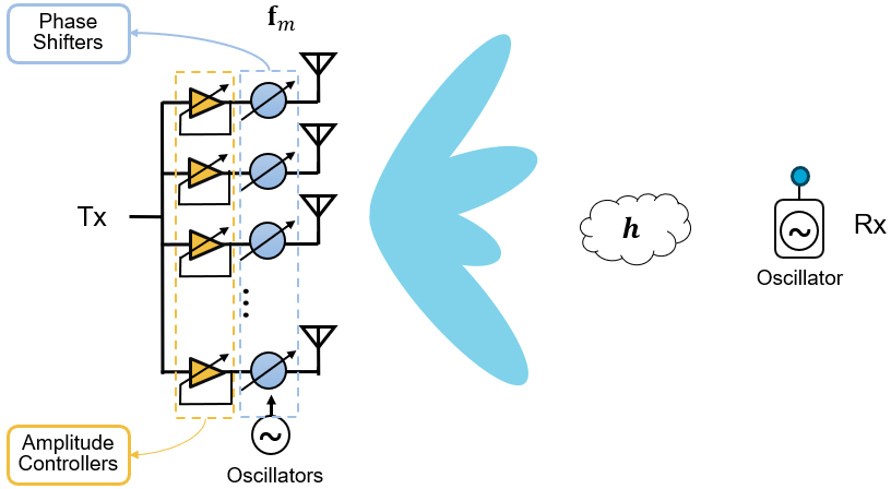
We consider a mmWave system with an analog antenna array comprising antennas at the transmitter (TX) and a single antenna receiver (RX) as shown in Fig. 1. The focus of this paper is on transmit beam alignment through channel estimation. Although we assume a single antenna at the RX for ease of exposition, our approach can be extended to multi-antenna receivers using an appropriate array response vector.
We consider a narrowband system and model the multiple input single output (MISO) channel between the TX and the RX as a vector . Let denote the number of propagation paths in the environment. The path gain and the direction of arrival associated with the path are denoted by and . Then, the channel is
| (1) |
Here, is the transmit array response vector given by
| (2) |
for a half-wavelength spaced uniform linear array at the TX. We use the discrete Fourier transform dictionary to obtain the angle-domain representation of the channel,
| (3) |
where is the unitary discrete Fourier transform matrix. The vector in (3) is sparse due to high scattering at mmWave carrier frequencies.
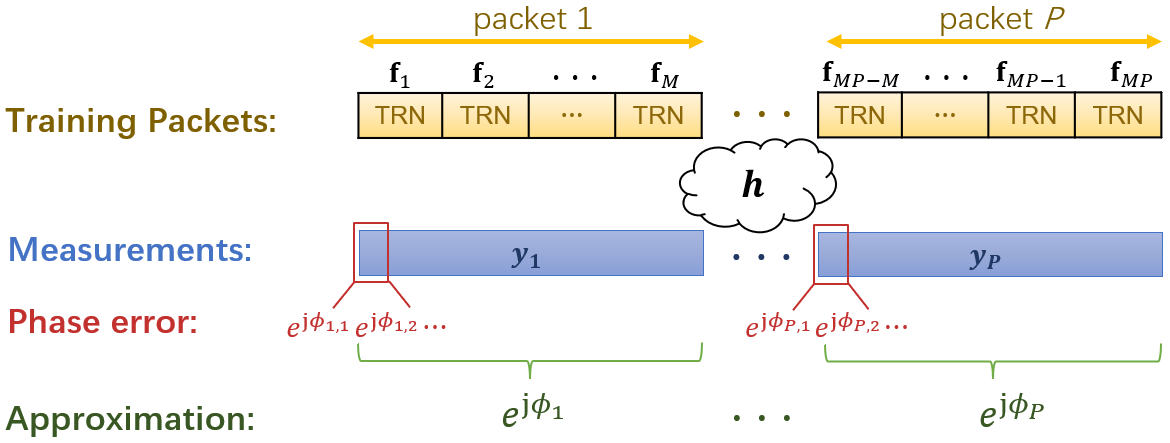
We next describe the frame structure used to obtain measurements for channel estimation. To this end, we consider the IEEE 802.11ad frame structure shown in Fig. 2. The TX applies distinct beamformers over different packets, for the RX to acquire channel measurements, within the channel coherence time. We define as the number of beamformers applied in each packet. With IEEE 802.11ad, can be at most [15]; however, it can often be smaller (e.g. ) to acquire redundant measurements and enhance the spreading gain. In that case, numerous beam refinement protocol (BRP) packets can be used to acquire enough spatial measurements for channel estimation.
Let denote the beamformer at the TX and denote the received channel measurement. This measurement is perturbed by phase noise and additive white Gaussian noise of variance , i.e.,
| (4) |
using (3). Note that is the conjugate transpose of . Here, the phase noise can be modeled as a Wiener process, i.e., , where is . Here, is the carrier frequency, is an oscillator-dependent constant, and is the time stamp associated with the measurement. Under these modeling assumptions, we aim to estimate the sparse channel using the measurements from (4) with the knowledge of , for .
III Sparse Channel Estimation Algorithm
In this section, we first reformulate the channel estimation problem into a CS problem to exploit the sparsity in and then, develop a greedy algorithm for channel estimation.
III-A Partially Coherent CS model
To formulate the CS model, we note that the time difference between successive measurements in a BRP packet, i.e., , is in IEEE 802.11ad. In contrast, the difference between the successive packets can range from s to s [16]. Therefore, a high variance phase offset is introduced in the measurements when switching to a new packet. Fig. 3 shows a realization of when measurements are acquired in each of the packets.
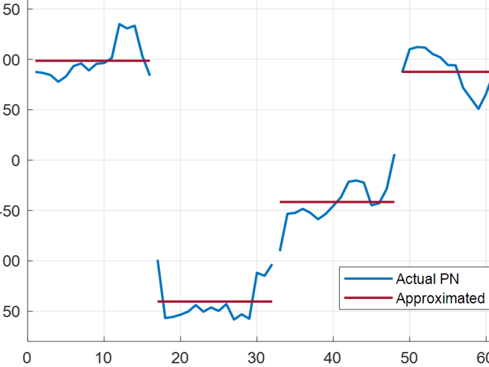
To develop a tractable algorithm, we ignore the phase variations within each packet and only consider phase offsets across different packets. In Sec. IV, however, we evaluate our algorithm by also considering phase variations within the packets.
Under the above simplifying assumption, the measurements can be expressed as a partially coherent CS model [12]. We define as the phase error in the measurements acquired within the packet. The vector of channel measurements, acquired over packets, can be expressed in terms of the CS matrix and the phase errors . Based on (4), we define the row of the CS matrix as
| (5) |
and a diagonal matrix containing the phase errors as where is a row vector comprising ones. The vector version of (4) is then
| (6) |
where and are unknown. We observe from (6) that can only be estimated up to a global phase. This is because is a solution to (6) whenever is a solution. Hence, the goal of partially coherent CS is to estimate , up to a global phase, from the measurements in (6).
We can split the measurement model in (6) on a packet-by-packet basis. The measurements from the packet correspond to rows to of (6). We define the measurements acquired in the packet as , and the CS measurement matrix associated with the packet as . Specifically, and
| (7) |
where is additive noise. Now, our channel estimation problem is equivalent to estimating from the phase perturbed measurements acquired using CS matrices .
III-B Partially coherent matching pursuit (PC-MP)
Our PC-MP algorithm is a greedy approach that adds one element to the estimated support set in each iteration. Then, the algorithm estimates the phase errors and the sparse signal over the estimated support through alternating minimization. This procedure is carried out until the stopping criterion is met. In this paper, we use the assumption in [12] that the number of non-zero coefficients in is known.
We first discuss our support detection rule in PC-MP. Our algorithm is initialized by setting to an empty set and to a zero vector. Here, we use to denote the estimated support set of the sparse vector, as the estimate of , and as the phase error estimated for packet , after iterations. The vector of estimated phase errors is denoted by . For the packet, we denote as the residual error between the observed measurements and the prediction in the iteration,
| (8) |
In the iteration, matching pursuit algorithms in standard CS identify the column of that results in the largest , i.e., the absolute value of the correlation with the residue. In our problem, however, we have different residues derived from packets. As the measurements across the packets are non-coherent, our algorithm sums up the absolute values of the correlations and selects the index that maximizes this summation. The new element added to the support set is
| (9) |
and the augmented support set is . For the special case when , we observe that the objective in (9) becomes identical to that used in matching pursuit algorithms for standard CS. In the iteration, our approach explicitly excludes support elements in while the OMP inherently avoids selecting such elements. This is because the residue in our approach may not be orthogonal to the selected columns of the CS matrix, unlike the OMP.
After the support estimation step, we use an alternating minimization approach to estimate the non-zero entries of over the identified support, and the phase errors . Our method minimizes the sum of the squared errors across all the packets to estimate these quantities,
| (10) |
where is a submatrix of obtained by retaining only those columns with indices in . We observe that (10) is a non-convex problem. It is, however, a standard least squares problem in for a fixed . Furthermore, a closed form solution for can be obtained for a fixed . Our alternating minimization procedure leverages both of these properties.
We now provide closed-form expressions for phase recovery and signal estimation in the iteration of alternating minimization in (10). For a fixed in (10), we observe that the minimization problem is separable in . The phase recovery problem for the packet is then
| (11) |
After estimating for each , the signal in (10) is estimated by solving a least squares problem. The solution is obtained by setting the gradient of the objective to and is given by
After the alternating minimization procedure converges in iterations, our method sets and . The subsequent PC-MP step updates the residue according to (8) and then identifies the next element of the support. A summary of our PC-MP technique is provided in Algorithm 1.
Now, we derive a coherence-based guarantee to successfully identify one element of the true support set of using PC-MP, for real-valued CS matrices.
Proposition 1.
Consider the channel estimation problem in (7) using measurements from packets. Assume that is real-valued with normalized columns, i.e., for each . For a constant , the support element identified in the first iteration of PC-MP is correct with probability exceeding
| (12) |
under the condition
| (13) |
where , is the coherence of [17], is the standard deviation of Gaussian additive noise , and is the sparsity level of .
Proof.
See the appendix. ∎
Intuitively, the result shows that support detection can only be successful under the assumption that the maximum absolute entry of is “larger” than the additive noise level as described by (13). Further, it also shows that a sufficient condition for successful identification of one element of the support in PC-MP’s first iteration is . Also, a good choice for the CS matrices for PC-MP is one with the lowest average coherence, i.e., .

IV Simulations
In this section, we compare the performance of our proposed method with OMP, self-calibration-based CS called Sparse-Lift [10], and partially coherent CS (PC-CPR) [12], considering the system model described in section II.
IV-A Benchmarking Algorithms
IV-A1 Reconstruction using Sparse-Lift
The idea in Sparse-Lift is to jointly estimate the calibration errors and the sparse vector by solving for a high-dimensional lifted matrix, which is an outer product of the error vector and the sparse vector. To apply Sparse-Lift, we define the calibration error vector as and the sparse vector is . The measurement vector in (6) is then
| (14) |
where . The entry of is given by
| (15) |
where is the row of and is the transpose of the row of . We define as the lifted matrix, which is sparse as is sparse. Using the identity , we can rewrite (15) as
| (16) |
which is a linear measurement of the lifted vector . With Sparse-Lift, measurements of this form are used to solve for the sparse matrix . Then, the singular value decomposition of the estimate is computed. The estimate of the sparse channel, up to a global scaling, is then , where is the conjugate of the singular vector corresponding to the largest singular value.
IV-A2 Partially Coherent Compressive Phase Retrieval (PC-CPR)
The partially coherent CS model in [12] assumes that the coherent measurements are acquired using different radio frequency chains. Although we consider a single radio frequency chain, our mathematical model is identical to the one in [12]. The algorithm in [12] is a two-stage method. In the first stage, the support set of the sparse vector is found by taking indices corresponding to the largest values of , where . Then, the sparse estimate is initialized using the eigen-decomposition-based method in [18]. In the second stage, the algorithm iteratively estimates the phase errors and the sparse signal. A hard thresholding algorithm is used to estimate the sparse signal.
IV-B Results and Discussion
We consider a uniform linear array of size at the TX. The standard deviation of phase noise, conditioned on the previous sample, is given as , with GHz as the carrier frequency, [4], and ns as the time duration of a single measurement in a packet. When computing the variance associated with the first sample of each packet, we use s. In our simulations, is exactly sparse with non-zero components drawn from a Gaussian distribution. We use random circularly shifted Zadoff-Chu sequences for the beamformers [7]. With this setup, spatial channel measurements are acquired in each of the packets.
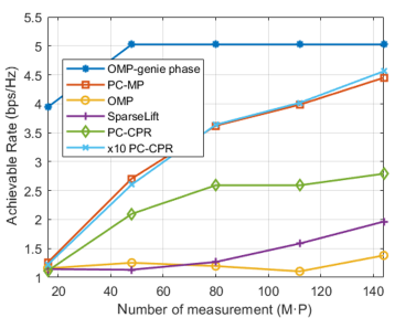
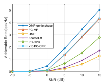
For the performance evaluation, we use the achievable rate as a metric and analyze how it varies with the SNR and the number of measurements. We define the SNR as and the achievable rate as , where is set to a unit-norm conjugate beamformer, i.e., . As the algorithms can estimate the channel only upto a global phase, we define the normalized mean squared error as . Our results are summarized in Fig. 4.
From the plots in Fig. 4, 4, and 4, we observe that standard OMP that works well with known phase errors (genie phase) breaks down under unknown practical phase noise. Next, we notice that the proposed PC-MP algorithm outperforms Sparse-Lift in terms of NMSE and the rate. This is because our algorithm exploits the constant magnitude structure in the calibration vector, unlike Sparse-Lift. Furthermore, we also observed that Sparse-Lift required substantially higher computation time than our approach, as it solves for a high dimensional lifted vector with variables. Our approach only solves for variables. Finally, we observe that the proposed PC-MP algorithm outperforms PC-CPR for the same iterations. This is likely due to the nature of the algorithms, i.e., PC-CPR is based on hard thresholding while our approach is based on matching pursuit. Both these algorithms assume a known sparsity level of . We would like to mention that the performance of PC-CPR for a large number of iterations ( PC-CPR) is close to our PC-MP method for iterations. For instance, PC-CPR required about iterations ( to achieve comparable performance as PC-MP for iterations (). These timings were observed in Matlab on a desktop computer. In summary, PC-MP can provide good channel estimates at a lower complexity than the benchmarks.
V Conclusions and Future Work
In this paper, we introduced a greedy algorithm called PC-MP for mmWave channel estimation under phase noise. Our approach makes use of the partially coherent structure in the phase perturbed measurements to perform sparse recovery and phase error estimation. PC-MP performs support detection by considering measurements from different packets, and iteratively estimates the sparse vector through alternating minimization. A comprehensive comparison revealed that PC-MP outperforms benchmark algorithms, yielding higher achievable rates and lower NMSE. We also derived guarantees on PC-MP’s performance in identifying one element from the true support. In future, we will extend our algorithm to account for off-grid effects and also analyze how well PC-MP can identify the entire support of the sparse vector.
Appendix: Proof of Proposition 1
We extend the support identification guarantee in [19] to the partially coherent case. Let be the true support of the sparse vector . Our proof verifies that when (13) holds,
| (17) |
which matches PC-MP’s detection rule to successfully identify one element of the support in its first iteration. To this end, we show that (17) holds under the event defined as
| (18) |
where controls the success probability of event . As is jointly Gaussian, we get
where is the Gaussian tail probability and the last step uses [20, theorem 1] for jointly Gaussian random variables. Further, since the Gaussian tail probability is bounded by we obtain
Substituting in the above relation shows that the event occurs with probability exceeding (12).
Once the event holds for , we can simplify the left-hand side of (17) as
| (19) | ||||
where the last step follows from (18) and the definition of and . For a sparsity level , using (7) and column normalization assumption on , we can bound the right-hand side of (17) as
| (20) | ||||
Here, from the definition of and , we get
| (21) |
In the first iteration of PC-MP, support identification is successful when (17) holds. We observe that the condition in (17) holds if the lower bound in (21) exceeds the upper bound in (19), which is equivalent to
| (22) |
which is the condition stated in (13).
Our guarantees are to identify only one element of the support set and not the entire support. This limitation is because of the residual errors arising due to joint phase recovery and signal estimation. These errors may not be orthogonal to the columns already selected, which prevents us from applying the induction argument discussed for the coherent case in [19].
References
- [1] B. K. J. Al-Shammari, I. Hburi, H. R. Idan, and H. F. Khazaal, “An overview of mmWave communications for 5G,” in Proc. Int. Conf. Commun. Inf. Technol., pp. 133–139, 2021.
- [2] Z. Chen, J. Tang, X. Y. Zhang, D. K. C. So, S. Jin, and K.-K. Wong, “Hybrid evolutionary-based sparse channel estimation for IRS-assisted mmWave MIMO systems,” IEEE Trans. Wirel. Commun., vol. 21, no. 3, pp. 1586–1601, 2022.
- [3] J. Zhu, D. W. K. Ng, N. Wang, R. Schober, and V. K. Bhargava, “Analysis and design of secure massive MIMO systems in the presence of hardware impairments,” IEEE Trans. Wirel. Commun., vol. 16, no. 3, pp. 2001–2016, 2017.
- [4] R. Zhang, B. Shim, and H. Zhao, “Downlink compressive channel estimation with phase noise in massive MIMO systems,” IEEE Trans. Commun., vol. 68, no. 9, pp. 5534–5548, 2020.
- [5] K. Venugopal, A. Alkhateeb, N. G. Prelcic, and R. W. Heath, “Channel estimation for hybrid architecture-based wideband millimeter wave systems,” IEEE J. on Sel. Areas in Commun., vol. 35, no. 9, pp. 1996–2009, 2017.
- [6] A. Alkhateeb, O. El Ayach, G. Leus, and R. W. Heath, “Channel estimation and hybrid precoding for millimeter wave cellular systems,” IEEE J. of Sel. Topics in Signal Process., vol. 8, no. 5, pp. 831–846, 2014.
- [7] N. J. Myers, A. Mezghani, and R. W. Heath, “Spatial zadoff-chu modulation for rapid beam alignment in mmwave phased arrays,” in Proc. of the IEEE Globecom Workshops (GC Wkshps), pp. 1–6, 2018.
- [8] H. Yan and D. Cabria, “Compressive sensing based initial beamforming training for massive MIMO millimeter-wave systems,” in Proc. IEEE Glob. Conf. Signal Inf. Process., pp. 620–624, 2016.
- [9] K.-H. Liu, X. Li, H. Zhao, and G. Fan, “Structured phase retrieval-aided channel estimation for millimeter-wave/sub-terahertz MIMO systems,” in Proc. IEEE Veh. Technol. Conf., pp. 1–5, 2022.
- [10] S. Ling and T. Strohmer, “Self-calibration and biconvex compressive sensing,” Inverse Problems, vol. 31, no. 11, p. 115002, 2015.
- [11] X. Li, J. Fang, H. Duan, Z. Chen, and H. Li, “Fast beam alignment for millimeter wave communications: A sparse encoding and phaseless decoding approach,” IEEE Trans. Signal Process., vol. 67, no. 17, pp. 4402–4417, 2019.
- [12] C. Hu, X. Wang, L. Dai, and J. Ma, “Partially coherent compressive phase retrieval for millimeter-wave massive MIMO channel estimation,” IEEE Trans. Signal Process., vol. 68, pp. 1673–1687, 2020.
- [13] C. Wei, H. Jiang, J. Dang, L. Wu, and H. Zhang, “Accurate channel estimation for mmWave massive MIMO with partially coherent phase offsets,” IEEE Commun. Lett., vol. 26, no. 9, pp. 2170–2174, 2022.
- [14] “IEEE standard for information technology–telecommunications and information exchange between systems - local and metropolitan area networks–specific requirements - part 11: Wireless LAN medium access control (MAC) and physical layer (PHY) specifications - redline,” IEEE Std 802.11-2020 (Revision of IEEE Std 802.11-2016) - Redline, pp. 1–7524, 2021.
- [15] “IEEE standard for information technology–telecommunications and information exchange between systems - local and metropolitan area networks–specific requirements - part 11: Wireless LAN medium access control (MAC) and physical layer (PHY) specifications,” IEEE Std, pp. 1–4379, 2021.
- [16] O. Kome, L. Cen, L. Hanqing, and Y. Rui, “Further details on multi-stage, multi-resolution beamforming training in 802.11 ay, doc,” 2016.
- [17] M. A. Davenport, M. F. Duarte, Y. C. Eldar, and G. Kutyniok, “Introduction to compressed sensing.,” 2012.
- [18] L. Zhang, G. Wang, G. B. Giannakis, and J. Chen, “Compressive phase retrieval via reweighted amplitude flow,” IEEE Trans. Signal Process., vol. 66, no. 19, pp. 5029–5040, 2018.
- [19] Z. Ben-Haim, Y. C. Eldar, and M. Elad, “Coherence-based performance guarantees for estimating a sparse vector under random noise,” IEEE Trans. Signal Process., vol. 58, pp. 5030–5043, Oct 2010.
- [20] Z. Sidak, “Rectangular confidence regions for the means of multivariate normal distributions,” J. Am. Stat. Assoc., vol. 62, no. 318, pp. 626–633, 1967.