Electronic States in Helical Materials:
General Properties and Application to InSeI

Abstract

In this article, we systematically explore several key properties of electronic states in helical materials systems, including the inheritance of orbital angular momentum (OAM) from local atomic orbitals to the entire helical structure, the conservation of helical momentum, and the emergence of helical-induced spin-orbit coupling (hSOC). We then apply this comprehensive theoretical framework to elucidate the electronic structure of one-dimensional (1D) helical crystal InSeI. Our analysis reveals the influence of hSOC, evident in spin-mixing energy gaps within the electronic band structure, as calculated through density functional theory. Utilizing a combination of tight-binding modeling and first-principles calculations, we ascertain the spin-polarized electric response and the chiral-switchable second-order photocurrent response of InSeI, characterized as the Landauer-Buttiker ballistic transport and shift current response. The results highlight the potential of 1D InSeI for applications in spintronics and optoelectronics. The overarching theoretical framework established in this work will prove invaluable for the investigation of other helical electronic systems.

Keywords

helical system; orbital angular momentum; spin-orbital coupling; spintronics; InSeI

I Introduction

Recently, helical materials, namely materials with atoms or atom groups arranged in a helical structure represented by the well-known DNA double helix, have attracted significant interest due to their unique geometry and properties. Unlike traditional planar systems, the atoms in a helical system are arranged both in planar (along the helical axis) and circular configuration (circumferential direction). Remarkably, the interplay between these planar and circular configurations introduces a non-trivial correlation that distinguishes them from typical tubular systems. This special feature leads to promising applications in electronic, optoelectronic, thermoelectric, and spintronic fields [1]. To harness the full potential of these advanced applications, it is imperative to conduct thorough investigations and gain a profound understanding of the electronic states within helical materials.

By now, extensive research has unequivocally confirmed that the electronic states in helical systems exhibit distinct properties. A pivotal aspect of the physics involved is the presence of chirality in helical structures, which leads to what is known as chiral-induced spin-selectivity (CISS) [2]. Several models in terms of spin-orbit coupling (SOC) have been proposed to describe CISS in systems resembling helix-shaped molecules [3], double-strand DNA [4, 5] and abstract helical system [6]. Additionally, Liu et al. [7] discussed the important role of orbital angular momentum (OAM) in DNA-like materials, achieving an OAM texture via a tight-binding model with expected topological implications. Furthermore, Hu et al. obtained a general expression for screw-symmetry-induced SOC through symmetry group analysis [8]. This expression was successfully applied to discuss the characteristic spin texture of dislocations in traditional semiconductors. These pioneering works have shed light on the unique electronic states in helical systems from diverse angles. However, a comprehensive and systematic description of electronic states in helical materials is still lacking. In addition, due to the intricate helical geometry, conventional modeling methods, such as the widely used tight-binding method, become complicated in describing realistic helical materials. This necessitates the development of adaptive methods for modeling helical materials systems.

Another significant consideration pertains to the categorization of materials within helical systems. In the early stages of research, the majority of helical materials that were discovered fell under the category of organic molecules, and consequently, most theoretical investigations have concentrated on these organic systems. However, as synthesis technologies have advanced, it has become possible to create a diverse array of inorganic crystal materials with helical structures, showcasing exceptional optical, electronic, and mechanical properties [9, 10, 11]. For example, InSeI represents a solid-state 1D helical crystal that has been both theoretically [12, 13] and experimentally [14] shown to exhibit high thermodynamic and chemical stability. It is expected to be a representative template of inorganic helical materials because it is composed of relatively heavy elements (In and Se) compared to organic materials (which are mainly composed of light elements such as C, H, and O). Additionally, the SOC effect in InSeI is stronger than in organic materials [12, 13]. However, only a limited number of theoretical studies have addressed helical InSeI, thereby impeding the comprehensive exploration of its potential applications.

Therefore, in this paper, we present a systematic discussion about electronic states in helical systems. The influences of helical structure independent from chemical details, such as the inheritance of OAM, conversation of helical momentum, and helical-induced SOC (hSOC), are discussed in a general case in section-II. These discussions are subsequently applied to the analysis of helical InSeI in section-III. This analysis not only establishes the validity of these principles by comparing them with DFT calculations but also delves into further properties specific to helical InSeI. Our work is expected to offer a comprehensive and systematic framework for modeling and understanding helical electronic systems.

II General case

II.1 “Tilted” local chemical environment

Figure 1: Comparison between planar and helical system. (a) Schematic of tetrahedron-type local chemical environment (highlighted in orange), and one example profile function (with phase labelled by different colors). (b) Schematic of identically polarized profile function in planar chain system, and tilted profile function in helical chain system.

Translational symmetry stands as a fundamental characteristic of solid-state crystal systems, governing the periodic arrangement of atoms. Within this framework, atoms occupying the same site share an identical local chemical environment, encompassing bonding and coordination, thereby inducing analogous local electronic hopping and hybridization behaviors. These shared characteristics dominantly influence the low-energy-effective physics [15]. Therefore, the tight-binding basis serves as a popular and reasonable starting point for analyzing the electronic states of solid-state crystal systems. The basis wavefunction is written as

$$\Psi_{\lambda\vec{k}}(\vec{r})={\sum\limits_{j}}e^{i\vec{k}{\cdot}\vec{R}_{j}}u_{\lambda}(\vec{r}-\vec{R}_{j})$$ (1)

where $j$ is the label of atomic site and $u_{\lambda}(\vec{r})$ is the localized profile function which has the same spatial period as the atomic site and is significantly localized at each atomic site (exponential decay). It is exclusively determined by the local chemical environment, similar to the maximally localized Wannier function scheme [16]. As shown in Fig. 1(a), one profile function with its phase labelled in different colors is centered at the black atomic site, which is surrounded by a tetrahedron-type local chemical environment (four nearest neighboring atoms in purple). In traditional planar systems, the local chemical environment of the same kind of site has the same spatial orientation, so does the profile function. This satisfies the tight-binding requirement. However, in helical materials (or more generally, in curved systems like carbon nanotubes), the local chemical environment of the same kind of sites may have different spatial orientations, i.e., they may be tilted to each other. This tilting of the local chemical environment also tilts the profile function, since the profile function must fit the configuration of the local chemical environment. As illustrated in Fig. 1(b), with only the black atomic sites plotted for simplicity, the profile functions are all polarized to $x$-direction in the planar chain system, but they are polarized to different directions in the helical chain system due to the tilted local chemical environment.

The tilting effect, which varies the polarization direction of the profile function at different sites, is of great importance since the directional polarization of the profile function reflects the orbital angular momentum (OAM). For example, the atomic $s$ orbital has no OAM (with an OAM angular quantum number of zero), resulting in a spherically symmetric profile without directional polarization. In contrast, atomic $p,d,f..$ orbitals with non-zero OAM exhibit polarized angular distributions to specific directions [17]. Consequently, the tilting of the chemical environment becomes relevant for these states. While the tilting effect exists in both tube and helical systems, the complexity in the latter arises from the arrangement of atomic site tilts in a global helical order. This helical order can couple the local and global properties of electronic states [18].

II.2 OAM inheritance

To comprehensively investigate the impact of tilted atomic sites on electronic states within helical systems and to develop an appropriate tight-binding modeling approach for such systems, let us consider a simplified scenario involving 1D helical material with an $\zeta$-fold screw symmetry. In this context, the system exhibits a sole screw structure and remains invariant under a screw symmetry operation denoted as $S_{z}[{\Delta}\varphi,a_{0}]=R_{z}[{\Delta}\varphi]{\cdot}T_{z}[a_{0}]$, operating along the screw axis ($z$-axis). Here $R_{z}[{\Delta}\varphi]$ is the rotational operation of ${\Delta}\varphi=2{\pi}/\zeta$ and $T_{z}[a_{0}]$ is the translational operation of distance $a_{0}$. The crystal unitcell can be evenly separated into $\zeta$ segments along the screw axis, which are identical in structure but different in spatial orientation, being titled by ${\pm}2{\pi}/\zeta$ along the screw axis relative to their nearest neighbors. These segments are defined as helical unitcells. Each helical unitcell is in length of $a_{0}$ thus the total crystal unitcell length is $\zeta{a_{0}}$. The system is also invariant after a single translational operation of distance $\zeta{a_{0}}$.

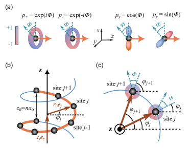
Figure 2: Atomic OAM and helical geometry. (a) Schematic of atomic $p$-orbitals with color-coded phases. (b), (c) Schematic illustrations defining the concept of helical atomic sites. The reference direction of local angular coordinate $\Phi$ (dashed green line) varies for different $j$, thus the same $\Phi$ value does not describe the same direction (dashed green arrow) globally. The spatial orientation angle of helical atomic site $\varphi_{j}$ is defined with the same global reference direction (black dashed line).

As illustrated in Fig. 2(b), let the origin of $j$-th helical unitcell be at the screw axis($z$-axis), with position vector $z_{j}\vec{e}_{z}$. For simplicity, we consider one atomic site inside each helical unitcell. The atomic site is located away from the screw axis with constant distance $r_{0}$ (which can be understood as the effective “section radius” of helical structure), but with different spatial orientation $\varphi_{j}$. To be more specific, the position of the $j$-th atomic site can be denoted as

$$\vec{r}_{j}=z_{j}\vec{e}_{z}+r_{0}\vec{e}_{j}$$ (2)

where $\vec{e}_{j}$ is the unit vector directed from the unitcell origin ($\vec{r}_{j}$) to the atomic site. As discussed above, $\varphi_{j{\pm}1}-\varphi_{j}={\pm}2{\pi}/\zeta$.

Recall that with local spherical coordinate $\vec{r}=(\rho,\theta,\Phi)$ centering at the atom, the atomic orbital basis $\psi$ can be written as

$$\psi_{nlm}(\vec{r})=A_{nl}(\vec{r})e^{im{\Phi}}$$ (3)

where $A_{nl}$ is the modulus part composed of radius and angular wavefunction. $n,l$ represents the main quantum number and angular quantum number while $m$ represents the OAM quantum number (also called the magnetic quantum number). The phase of $\psi_{nlm}$ is totally offered by $m$. For example, as for $p$ orbitals we have [17]

$$|0{\rangle} =\sqrt{2}R_{n1}(\rho)\cos{\theta}$$ (4)

$$|{\pm 1}{\rangle} =-R_{n1}(\rho)\sin{\theta}e^{{\pm}i{\Phi}}$$

where $R_{n1}(\rho)$ is the radius part. A clear $e^{{\pm}i{\Phi}}$ term can be observed, which means that the phase of $\psi_{nl}$ differs in local angular coordinate $\Phi$ as the schematic shown in Fig. 2. We may be more familiar with their linear combinations with a symmetric form to $x,y,z$ directions as

$$p_{x} =\frac{1}{\sqrt{2}}(|-1{\rangle}+|+1{\rangle})=\sqrt{2}R_{n1}(\rho)\sin{\theta}\cos({\Phi})$$ (5)

$$p_{y} =\frac{i}{\sqrt{2}}(|-1{\rangle}-|{+1}{\rangle})=\sqrt{2}R_{n1}(\rho)\sin{\theta}\sin({\Phi})$$

$$p_{z} =|0{\rangle}=\sqrt{2}R_{n1}(\rho)\cos{\theta}$$

In a helical system, it is not straightforward to directly employ $\psi_{nlm}$ in the form shown in Eq. 3 as the profile function to plug into tight-binding basis Eq. 1. The challenge arises from the fact that the reference direction of the local rotational coordinate $\Phi$ differs at different sites, rendering $\Phi$ not well-defined globally. To illustrate it further, let’s align the axis of $\Phi$ parallel to the screw axis (along $z$-direction) without loss of generality. As shown in Fig. 2(b), since the spatial orientation of site $j$ is different from that of site $j+1$, i.e. $\varphi_{j}\neq\varphi_{j+1}$, the reference directions of $\Phi$ at site $j$ and $j+1$ (drawn as green dashed lines) are also different. This means that even the same $\Phi$ value actually refers to different directions (drawn as green dashed arrows). To fix this problem, we can subtract the site orientation $\varphi_{j}$ from $\Phi$ to replace $\Phi$ by its globally well defined counterpart $\Phi-\varphi_{j}$. This is not just a mathematical trick, but it reflects the physical reality that the local rotational degree of freedom, $\Phi$, is not as trivially identical for all the atomic sites as in planar systems, but becomes coupled to the global rotational degree of freedom $\varphi$ in helical systems. With this consideration, based on Eq. 1, Eq. 3 and the site vector defined in Eq. 2, we can write down the tight-binding basis as

$$\Psi_{nl,km}(\vec{r}) ={\sum\limits_{j}}e^{ikz_{j}}A_{nl}(\vec{r}-\vec{r}_{j})e^{im(\Phi-\varphi_{j})}$$ (6)

$$={\sum\limits_{j}}[e^{ikz_{j}}e^{-il\varphi_{j}}][A_{nl}(\vec{r}-\vec{r}_{j})e^{im\Phi}]$$

$$={\sum\limits_{j}}{\langle}X_{j}|\Omega_{kl}{\rangle}\psi_{nlm}(\vec{r}-\vec{r}_{j})$$

where ${\langle}X_{j}|$ is the position basis of unitcell $j$. In the last line, the influence of helical structure to the phase of $\Psi_{nl,km}$, or in other words the $j$-dependent part, has totally been organized into $\Omega_{kl}$ defined as

$$\Omega_{km}(z,\varphi)=e^{ikz}e^{-im\varphi}$$ (7)

so that the local part $\psi_{nlm}(\vec{r}-\vec{r}_{j})=A_{nl}(\vec{r}-\vec{r}_{j})e^{im\Phi}$ goes back to the pure atomic orbital form described in Eq. 3. It can be observed that the OAM $m$ is originally only carried by the local rotational degree of freedom $\Phi$ of the atomic orbital. However, due to the tilted local chemical environment, $m$ is also carried by the directional polarization angle $\varphi_{j}$ of the helical atomic site, which belongs to a global degree of freedom. In other words, the atomic OAM is “inherited” by the helical structure.

It is essential to emphasize that since $\Phi$ ranges continuously from 0 to $2\pi$ while $\varphi_{j}$ can only take discrete values $\varphi_{j}=2{\pi}j/\zeta,j=0,1,2,...,\zeta-1$, the OAM inheritance cannot be complete because any state with $|m|=m^{\prime}+[\zeta/2]>[\zeta/2]$ ($[...]$ means round down), the following relation is always valid

$$e^{-im\varphi_{j}} =e^{{\pm}i(m^{\prime}+[\zeta/2])\varphi_{j}}=e^{{\pm}im^{\prime}\varphi_{j}}e^{{\pm}i{\pi}j}$$ (8)

$$=e^{{\pm}im^{\prime}\varphi_{j}}e^{{\mp}i{\pi}j}=e^{{\pm}i(m^{\prime}-[\zeta/2])\varphi_{j}}$$

which means any state with $|m|>[\zeta/2]$ is actually equivalent to another state with $|m|<[\zeta/2]$. In other words, the number of distinct $m$ that can be inherited is limited by screw symmetry order $\zeta$ as

$$m=0,\pm 1,\pm 2,...,\pm[\zeta/2]$$ (9)

As an instance, since in a $\zeta=3$ helical system distinct $m$ are only $0,\pm 1$, a $d$ atomic orbital with $m=\pm 2$ can not be totally inherited but is equivalent to a $m=\pm 1$ states. This is also the reason why the inherited OAM is commonly called the quasi-OAM just like the crystal momentum ${\hbar}k$ is called the quasi-momentum.

It is straightforward to verify that $\Psi_{nlm}$ in Eq. 6 satisfies the screw symmetry $S_{z}[{\Delta}\varphi,a_{0}]=R_{z}[{\Delta}\varphi]{\cdot}T_{z}[a_{0}]$, just as the common Bloch wave satisfies the translational symmetry as shown in Eq. 10

$$\begin{aligned} &S_{z}[{\Delta}\varphi,a_{0}]{\cdot}\Psi_{nl,km}(\vec{r})\\ &=R_{z}[{\Delta}\varphi]{\cdot}T_{z}[a_{0}]{\cdot}{\sum\limits_{j}}e^{ikz_{j}}A_{nl}(\vec{r}-z_{j}\vec{e}_{z}-r_{0}\vec{e}_{j})e^{im(\Phi-\varphi_{j})}\\ &={\sum\limits_{j}}e^{ikz_{j}}A_{nl}(\vec{r}+a_{0}\vec{e}_{z}-z_{j}\vec{e}_{z}-r_{0}\vec{e}_{j-1})e^{im(\Phi-\varphi_{j}+{\Delta}\varphi)}\\ &=e^{ika_{0}}\Psi_{nl,km}(\vec{r}).\end{aligned}$$ (10)

Considering the macroscopic periodic condition (Born-von Karman boundary condition), the wavefunction should be invariant after being translated through a distance of $N{\zeta}a_{0}$ ($N$ is a large integer number)

$$\Psi_{nl,km}(\vec{r}+N{\zeta}a_{0}\vec{e}_{z})$$ (11)

$$=T[N{\zeta}a_{0}]{\cdot}\Psi_{nl,km}(\vec{r})$$

$$=S_{c}[N{\zeta}a_{0},N{\zeta}{\Delta}\varphi]{\cdot}\Psi_{nl,km}(\vec{r})$$

$$=S_{c}[a_{0},{\Delta}\varphi]^{N{\zeta}}{\cdot}\Psi_{nl,km}(\vec{r})$$

$$=e^{ikN{\zeta}a_{0}}\Psi_{nl,km}(\vec{r})$$

$$=\Psi_{nl,km}(\vec{r})$$

which gives us the $1^{\rm st}$ Brillouin zone (BZ) of crystal unitcell

$$e^{ikN{\zeta}a_{0}}=1\ \ {\Rightarrow}\ \ k=\frac{\gamma}{N}\frac{2\pi}{{\zeta}a_{0}},\gamma{\in}[-N/2,N/2]$$ (12)

II.3 Helical momentum

In this section, we derive the hopping and hybridization parameters of the crystal Hamiltonian $H$ connecting $|\Psi_{k^{\prime}l^{\prime}n^{\prime}}{\rangle}$ and $|\Psi_{kln}{\rangle}$ as follows:

$${\langle}\Psi_{nl,km}|H|\Psi_{n^{\prime}l^{\prime},k^{\prime}m^{\prime}}{\rangle}={\sum\limits_{j,j^{\prime}}}e^{-ikz_{j}}e^{im\varphi_{j}}e^{ik^{\prime}z_{j}}e^{-im^{\prime}\varphi_{j}}$$ (13)

$$\ \ \ {\times}{\int}{\psi_{nl}^{*}(\vec{r}-\vec{r}_{j}-r_{0}\vec{e}_{j})}H{\psi_{n^{\prime}l^{\prime}}(\vec{r}-\vec{r}_{j^{\prime}}-r_{0}\vec{e}_{j^{\prime}})}d\vec{r}.$$

The integral of local profile function $\psi_{nl}$, $\psi_{n^{\prime}l^{\prime}}$ yields to the Slater-Koster (SK) coefficient, denoted as $t^{\tau}_{ll^{\prime}nn^{\prime}}$. This coefficient is solely determined by local chemical composition of the material. The index $\tau$ serves to replace $j^{\prime}$ and represents the site’s neighboring site $j$. For example, $\tau=0$ corresponds to on-site hybridization and $\tau=\pm 1$ refers to the nearest neighboring hopping. We further use the helical geometry relations $z_{j}=ja_{0}$, $\varphi_{j}=j{\Delta}\varphi=j(2\pi/{\zeta}a_{0})$; ${\Delta}z_{\tau}={\tau}a_{0}$, ${\Delta}\varphi_{\tau}={\tau}{\Delta}\varphi={\tau}(2\pi/{\zeta}a_{0})$ and define ${\Delta}m=m^{\prime}-m,\bar{m}=(m^{\prime}+m)/2$; ${\Delta}k=k^{\prime}-k,\bar{k}=(k^{\prime}+k)/2$, so that we have

$${\langle}\Psi_{nl,km}|H|\Psi_{n^{\prime}l^{\prime},k^{\prime}m^{\prime}}{\rangle}$$ (14)

$$\begin{aligned} &={\sum\limits_{j}}e^{i({\Delta}kz_{j}-{\Delta}m\varphi_{j})}\\ &\ \ \ {\times}{\sum\limits_{\tau}}\frac{t_{ll^{\prime}nn^{\prime}}^{\tau}}{2}[e^{ik^{\prime}{\Delta}z_{\tau}}e^{-im^{\prime}{\Delta}\varphi_{\tau}}+(km{\leftrightarrow}k^{\prime}m^{\prime})]\end{aligned}$$

$$\begin{aligned} &={\sum\limits_{j}}e^{i({\Delta}ka_{0}-{\Delta}m{\Delta}\varphi)j}\\ &\ \ \ {\times}{\sum\limits_{\tau}}t_{ll^{\prime}nn^{\prime}}^{\tau}\cos[\frac{1}{2}({\Delta}ka_{0}-{\Delta}m{\Delta}{\varphi}){\tau}]e^{i(\bar{k}a_{0}-\bar{m}{\Delta}\varphi){\tau}}\end{aligned}$$

$$={\delta}({\Delta}k-{\Delta}m\frac{2{\pi}}{{\zeta}a_{0}}){\sum\limits_{\tau}}t_{ll^{\prime}nn^{\prime}}^{\tau}e^{i(\bar{k}-\bar{m}\frac{2\pi}{{\zeta}a_{0}})a_{0}{\tau}}$$

The first difference between Eq. 14 and hopping in a planar system [19] is the conservation law. In a planar crystal, the wave-vector $k$ is a good quantum number, which means that no hybridization happens between two different $k$-states and the crystal momentum $\hbar{k}$ is conserved. However, in a helical system, the conserved quantity is the helical momentum ${\hbar}L$ defined as

$$\hbar{L}=\hbar({k}-mG)\ \ \ G=2\pi/{\zeta}a_{0}$$ (15)

which is composed of both crystal momentum and OAM. The phase factor of the hopping parameter in Eq. 14 is also determined by $L$ instead of only $k$, which agrees well with previous work [7] while they explained the influence of $m$ as anisotropic hopping without a detailed discussion on the origin and extension to the general case.

The helical momentum can be defined in two schemes. In the crystal BZ scheme, with wavevector $|k|<{\pi}/{\zeta}a_{0}$, as shown in Eq. 11, $L$ is written as Eq. 15 composed of both $k$ and $m$. Since $k$-space is periodic with BZ size $2\pi/{\zeta}a_{0}$, i.e. $k$-states modulo $2\pi/{\zeta}a_{0}$ are identical, the conservation relation ${\Delta}L=0$ is actually equivalent to ${\Delta}k=0,{\Delta}m=0$ in this case. In the helical BZ scheme, with wavevector $|K|<{\pi}/a_{0}$ and helical BZ length $2\pi/a_{0}>2\pi/{\zeta}a_{0}$, we could separate $K$ into $K=k+pG,p\in{\mathbb{Z}}$ still with $k<|2\pi/{\zeta}a_{0}|$ and $p$ is the maximum common divisor of $k$ over $G$. Note that $K$ in helical momentum shares the same form with $L$ in crystal BZ scheme, and $p$ plays the same role with $-m$. Also, since these two schemes actually describe the same Hilbert space, the helical momentum in the helical BZ scheme is simply $L=K$. Therefore, in the helical BZ scheme, the linear crystal momentum $\hbar{k}$ and OAM $\hbar{m}$ are coupled together so that any two states $|k,m{\rangle}$ and $|k\ {\pm}\ pG,m\ {\mp}\ p{\rangle},p{\in}\mathbb{Z}$ share the same $L$ and are thus identical. This is a direct result of screw symmetry. Due to the same reason, the two BZ definitions can be continuously transformed to each other. This gives us a method to conveniently identify $L$ for each state. First, we obtain the energy bands in the first crystal BZ, as is commonly done in ab initio calculations. Second, as discussed in the beginning of section-II.2, we extend the first crystal BZ into $\zeta$-times larger to obtain the helical BZ. During this process, the energy bands are also unfolded continuously, so that each band with specific $k,m$ defined in crystal BZ is shifted to wavevector $K=k-mG=L$ in helical BZ. Therefore, we can identify the helical momentum $L$ and corresponding OAM $m$ by checking the location of the unfolded band in helical BZ. An example can be found in section-III.1.

To address the physical picture of $L$-conservation, let us consider the umklapp process as an example. In a planar system, an electron can only be scattered across the whole crystal BZ if the momentum transfer is nonzero, such as in an electron-electron or electron-phonon interaction. However, in a helical system, the scattering medium can be momentum-free or in the long-wave limit, because there is another way to achieve the scattering by exchanging the linear crystal momentum and OAM. This can be done by transitioning between the states $|k,m{\rangle}$ and $|k\ {\pm}\ pG,m\ {\mp}\ p{\rangle},p{\in}\mathbb{Z}$, which does not require any external momentum supply. In terms of the Feynman diagram, this additional path can open up new possibilities for scattering processes. It can also make some previously insignificant diagrams more important. This could have a significant impact on many-body interactions, and it is worth further investigation.

II.4 Chirality

One of the important properties of helical structures is their chirality, which means that the structure is distinguishable from its mirror image. Intuitively, the left/right-hand chiral helix can be constructed by rolling a chain in a clockwise/anticlockwise direction along the helical axis. Based on the geometric interpretation of the helical structure defined above, namely the linear coordinate $z_{j}$ and angular coordinate $\varphi_{j}$ of $j$-th atomic site, the influence of chirality to helical geometry can be reflected as an additional coupling sign $\nu=\pm 1$ that

$$z_{j}=ja_{0},\ \varphi_{j}=\nu{j}{\Delta}\varphi$$ (16)

or equivalently $z_{j}={\nu}ja_{0},\ \varphi_{j}={j}{\Delta}\varphi$. A direct result can be found in Eq. 14 that the conserved helical momentum becomes

$$\hbar{L}=\hbar(k-{\nu}mG)$$ (17)

For example, $p_{+}$ state with $m=+1$ will be inherited to helical momentum as $\hbar(k-mG)$ and $\hbar(k+mG)$ in different chiral system respectively.

Besides, the non-zero Berry phase arising from the inversion symmetry breaking along the helical axis is also dependent on the chirality of the helix, which can be calculated as

$$\gamma={\sum\limits_{E_{j}<E_{f}}}\int_{-\pi/{\zeta}a_{0}}^{\pi/{\zeta}a_{0}}{\langle}\kappa_{j}|\frac{{\partial}}{\partial{k}}|\kappa_{j}{\rangle}dk$$ (18)

where the summation is over all the occupied eigen-states $|\kappa_{j}{\rangle}$ with energy $E_{jk}$ smaller than Fermi energy $E_{f}$. In the tight-binding representation, $|\kappa_{j}{\rangle}$ is a linear combination of tight-binding basis defined in Eq. 6 as

$$|\kappa_{j}{\rangle}={\sum_{nlm}}c_{j;nl,km}|\Psi_{nl,km}{\rangle}$$ (19)

where $c_{j;nl,km}$ is the superposition coefficient representing the hybridization between different basis and is determined by the material structure. If the chirality is reversed from $\nu=+1$(-1) to $\nu=-1$(+1), the only difference in the material structure is the sign of the $z$-coordinate. This results in a change of global phase factor changes from $e^{ikz}$ to $e^{-ikz}$, which is equivalent to changing $k$ into $-k$. Therefore, the operator ${\partial}_{k}$ in Eq. 18 becomes ${\partial}_{-k}=-{\partial}_{k}$. Another way to understand sign reverse is that the $z$-position operator is defined as $\hat{z}=-i{\partial}_{k}$. Therefore, changing the chirality from $\nu=+1$(-1) to $\nu=-1$(+1) is equivalent to changing $\hat{z}$ to $-\hat{z}$. As a conclusion, the Berry phase of structures with opposite chirality should have opposite signs. Correspondingly, the physical quantities related to the Berry phase, such as electric polarization and second-order nonlinear optical responses, e.g., shift current, will also have opposite signs for structures with opposite chirality, which makes chirality an experimentally detectable and measurable property.

II.5 Helical-induced SOC

It is worth noting that the helical arrangement of atoms is non-trivial, regardless of the chemical details at each atomic site. This is because it creates a potential field that is strong near the helical structure but weak in other regions. In this section, we will show that this helical-shaped potential leads to a spin-orbital coupling (SOC). Consider a helical potential $V_{h}$ defined on the cylindrical coordinate system $(\varphi,z)$ as

$$V_{h}=V_{0}\exp[-\alpha{\sin}^{2}({\pi}\frac{z}{z_{0}}+{\nu}\frac{\varphi}{2}+\frac{\varphi_{0}}{2})]$$ (20)

where $\alpha>0$ controls the potential width, $\nu=\pm 1$ represents different chirality as is defined in Eq. 16 and $\varphi_{0}$ is a phase constant. $V_{h}$ is periodic on both $z$ and $\varphi$ with period $z_{0}$ and $2\pi$, respectively. For the helical trajectory used in Eq. 14 that the coordinate of $j$-th atomic site is $z_{j}=ja_{0},\varphi_{j}=-2{\nu}j\pi/\zeta$ (${\zeta}a_{0}=z_{0}$), The value of $V_{h}$ is constant, as are the gradients of $V_{h}$ in the $z$ and $\varphi$ directions, $E_{z0}=\partial_{z}{V_{h}}$ and $E_{t0}=\partial_{r_{0}{\varphi}}{V_{h}}$

$${\nabla}V_{h} =\pmb{e_{z}}E_{z0}+\pmb{e_{t}}{\nu}E_{t0}$$ (21)

$$E_{t0} =-{\alpha}(\frac{1}{r_{0}})V_{0}\exp[-\alpha\sin(\varphi_{0}/2)^{2}]\sin(\varphi_{0})$$

$$E_{z0} =-{\alpha}(\frac{2\pi}{z_{0}})V_{0}\exp[-\alpha\sin(\varphi_{0}/2)^{2}]\sin(\varphi_{0})$$

where $\pmb{e_{z}}$ and $\pmb{e_{t}}$ are unit vectors along the $z$- and circumferential directions, respectively, and $r_{0}$ is the (effective) radius of helical section. The SOC operator arising from helical potential $V_{h}$ is written as

$$\hat{H}_{SO}=-{\xi}\hat{\pmb{\sigma}}{\cdot}({\nabla}V_{h}{\times}\hat{\pmb{p}})$$ (22)

with constant $\xi={g\mu_{B}}/{2mc}$. The momentum operator $\hat{\pmb{p}}$ can also be projected along the two directions as

$$\hat{\pmb{p}} =\pmb{e_{z}}\hat{p}_{z}+\pmb{e_{t}}\hat{p}_{t}$$ (23)

$$\hat{p}_{z} =(-i{\hbar})\frac{\partial}{\partial{z}}\ \ \ \hat{p}_{t}=(-i{\hbar})\frac{\partial}{{r_{0}}\partial{\varphi}}$$

We get the following expression from Eq. 22 for the SOC Hamiltonian

$$H_{SO} =-{\xi}\hat{\pmb{\sigma}}{\cdot}[(\pmb{e_{z}}E_{z}+\pmb{e_{t}}E_{t}){\times}(\pmb{e_{z}}\hat{p}_{z}+\pmb{e_{t}}\hat{p}_{t})]$$ (24)

$$=-\xi\hat{\pmb{\sigma}}{\cdot}\pmb{e_{r}}(E_{t}\hat{p}_{z}-E_{z}\hat{p}_{t})$$

$$=-\xi\hat{\sigma}_{s}(E_{t}\hat{p}_{z}-E_{z}\hat{p}_{t})$$

where $\pmb{e}_{r}=\pmb{e}_{t}{\times}\pmb{e}_{z}$ is the unit vector along the radius direction. It can be found that this helical-induced SOC (hSOC) arises from the inversion symmetry breaking along both the circumferential and helical-axis directions. The spin operator $\hat{\sigma}_{s}=\hat{\pmb{\sigma}}{\cdot}\pmb{e_{r}}$ is calculated as

$$\hat{\pmb{\sigma}}{\cdot}\pmb{e_{r}} =\hat{\sigma}_{x}\cos(\varphi)+\hat{\sigma}_{y}\sin(\varphi)$$ (25)

$$=e^{i{\varphi}}\frac{\hat{\sigma}_{x}-i\hat{\sigma}_{y}}{2}+e^{-i{\varphi}}\frac{\hat{\sigma}_{x}+i\hat{\sigma}_{y}}{2}$$

$$=e^{i{\varphi}}{\hat{\sigma}_{+}}+e^{-i{\varphi}}{\hat{\sigma}}_{-}$$

$$\hat{\sigma}_{+} =\frac{\hat{\sigma}_{x}-i\hat{\sigma}_{y}}{2}\ \ \ \ \hat{\sigma}_{-}=\frac{\hat{\sigma}_{x}+i\hat{\sigma}_{y}}{2}$$

where $\hat{\sigma}_{x,y,z}$ are Pauli operators.

Without considering the local details (profile function), we only keep the global part of the tight-binding basis defined in Eq. 7. Further combining with the spinor $|\chi{\rangle}$, we have the basis state as $|\chi,k,m{\rangle}{\equiv}|\Omega_{km}{\rangle}|\chi{\rangle}=e^{ikz}e^{-im\varphi}|\chi{\rangle}$. The atomic sites on the helical trajectory are $z_{j}=ja_{0},\varphi_{j}=-2{\nu}j\pi/\zeta$. The matrix element of $H_{SO}$ can be calculated as

$${\langle}{\chi_{1}},k_{1},m_{1}|\hat{H}_{SO}|\chi_{2},k_{2},m_{2}{\rangle}$$ (26)

$$=-{\xi}{\hbar}[{\nu}E_{t0}k_{2}-\frac{E_{z0}}{r_{0}}(-{\nu})(-m_{2})]{\sum\limits_{j}}e^{i({\Delta}kz_{j}-{\Delta}m\varphi_{j})}{\langle}\hat{\sigma}_{s}{\rangle}$$

$$=-{\xi}{\nu}E_{t0}{\hbar}(k_{2}-m_{2}G){\sum\limits_{\pm}}{\sum\limits_{j}}e^{i[{\Delta}ka_{0}+({\Delta}m{\pm}1)\frac{2\pi}{\zeta}]j}{\langle}\hat{\sigma}_{\pm}{\rangle}$$

$$=-{\xi}{\nu}E_{t0}{\hbar}(k_{2}-m_{2}G){\sum\limits_{\pm}}{\delta}[{\Delta}k+({\Delta}m{\pm}1)G]{\langle}\hat{\sigma}_{\pm}{\rangle},$$

where ${\Delta}k=(k_{2}-k_{1})/2$ and ${\Delta}m=[(-m_{2})-(-m_{1})]/2=(m_{1}-m_{2})/2$. It’s important to note that the term $\frac{E_{z0}}{r_{0}}(-{\nu})(-m_{2})$ in the first equality arises from the action of the operator $\hat{p}_{t}|\chi_{2},k_{2},m_{2}{\rangle}$. The presence of the factor $-\nu$ is a result of the fact that $|\chi_{2},k_{2},m_{2}{\rangle}$ is situated along the helix with a $\varphi$-variation dependent on $-\nu$ (recalling that $\varphi_{j}=-2{\nu}j\pi/\zeta$). Consequently, when calculating $\partial_{\varphi}e^{-im\varphi}$, the factor of $-\nu$ is unavoidable.

Notice that Eq. 27 is not Hermitian, because the strength is not symmetric to $m_{1},m_{2}$ since $m_{1}{\neq}m_{2}$. Also, with $k$ defined in $|k|<G=2\pi/{\zeta}a_{0}=2\pi/z_{0}$, the selection rule ${\delta}[{\Delta}k+({\Delta}m{\pm}1)G]$ becomes ${\delta}({\Delta}k)\delta({\Delta}m{\pm}1)$. We can define the corresponding Hermitized hSOC matrix element as

$$H_{SO} =-{\xi}{\nu}E_{t0}\bar{L}{\sum\limits_{\pm}}{\delta}({\Delta}k){\delta}({\Delta}m{\pm}1){\langle}\hat{\sigma}_{\pm}{\rangle}$$ (27)

$$\bar{L} =\hbar({k}-\frac{m_{1}+m_{2}}{2}G)$$

The strength of $H_{SO}$ is composed of three parts. The first one is the on-helix circumferential potential gradient $E_{t0}$, which is the effective electric field along the circumferential direction. The second one is the chirality factor $\nu$, which means that the sign of $H_{SO}$ is different for opposite chiralities. The last one is the (averaged) helical momentum $\bar{L}$, which restricts $\bar{L}(k)=-\bar{L}(-k)$ in order to satisfy the time-reversal symmetry. In other words, the sign of OAM $m$ is directly coupled to that of $k$. It can also be observed that $H_{SO}$ transforms the helical momentum $L$ with spin angular momentum (as shown in Eq. 26) so that $H_{SO}$ is spin-flipping. The summation over ${\pm}$ in Eq. 27 contains two cases, the lifting of spin angular momentum (${\langle}\hat{\sigma}_{+}{\rangle}$) together with the lowering of helical momentum (${\Delta}L=-\hbar{G}$), and the lowering of spin angular momentum (${\langle}\hat{\sigma}_{-}{\rangle}$) together with the lifting of helical momentum (${\Delta}L=+\hbar{G}$). Both cases conserve the angular momentum. All these features are quite similar to other kinds of symmetry-breaking SOC, such as the widely acknowledged Dresselhaus-Rashba SOC in planar systems [20]. The strength of Dresselhaus-Rashba SOC is proportional to the crystal momentum and the effective electric field that arises from the broken inversion symmetry. This comparison suggests that the helical momentum in helical systems plays the same role as the crystal momentum does in planar systems.

The hSOC can also be understood and estimated in a semi-classical way. Consider a quasi-electron with effective mass $m_{e}^{*}$ passing through the ions arranged along a helical chain with axis towards $z$-direction, screw pitch $z_{0}$ and radius $r_{0}$. As the feature of helix, the electron should simultaneously have a linear motion with velocity $v_{z}={\hbar}k/m_{e}^{*}$ and a rotational motion with angular velocity $\omega$. Once the electron covers a distance $z_{0}$ in $z$-direction, it should go through 2${\pi}$ in the circular direction, which means that they share the same time period $T=z_{0}/v_{z}=2{\pi}/\omega$ so that $\omega=2\pi{\hbar}k/m_{e}^{*}z_{0}$. Recall that the classical OAM is $m_{e}^{*}\omega{r_{0}^{2}}$, we can calculate the OAM quantum number as

$$\hbar{m^{\prime}}=m_{e}^{*}{\omega}r_{0}^{2}=\frac{2{\pi}{\hbar}r_{0}^{2}}{z_{0}}k$$ (28)

where $m^{\prime}=2k{\pi}r_{0}^{2}/z_{0}$ is proportional to $k$. In the rest reference framework of the electron, the ions rotate relative to the electron, which induces a magnetic field with the magnetic induction strength along the $z$-direction as $B_{z}$. The strength of the electrostatic interaction is denoted by the effective electric field intensity $E_{0}$ along the radius direction. We obtain $B_{z}\ {\sim}\ E_{0}\omega/2c^{2}$. Therefore, the spin magnetic moment $\mu_{s}=e{\hbar}s_{z}/2m_{e}^{*}$, with spin quantum number $s_{z}{\in}[-1/2,1/2]$, is coupled with linear momentum $\hbar{k}$ (as long as the OAM $m^{\prime}$) with the strength $\lambda_{R}$ as

$${\lambda_{R}}=\mu_{s}B_{z}=\frac{E_{0}{\hbar^{2}}{\pi}e}{2m_{e}^{*2}c^{2}z_{0}}ks_{z}=\frac{{\beta}}{z_{0}}ks_{z}$$ (29)

III Application to InSeI

III.1 OAM inheritance

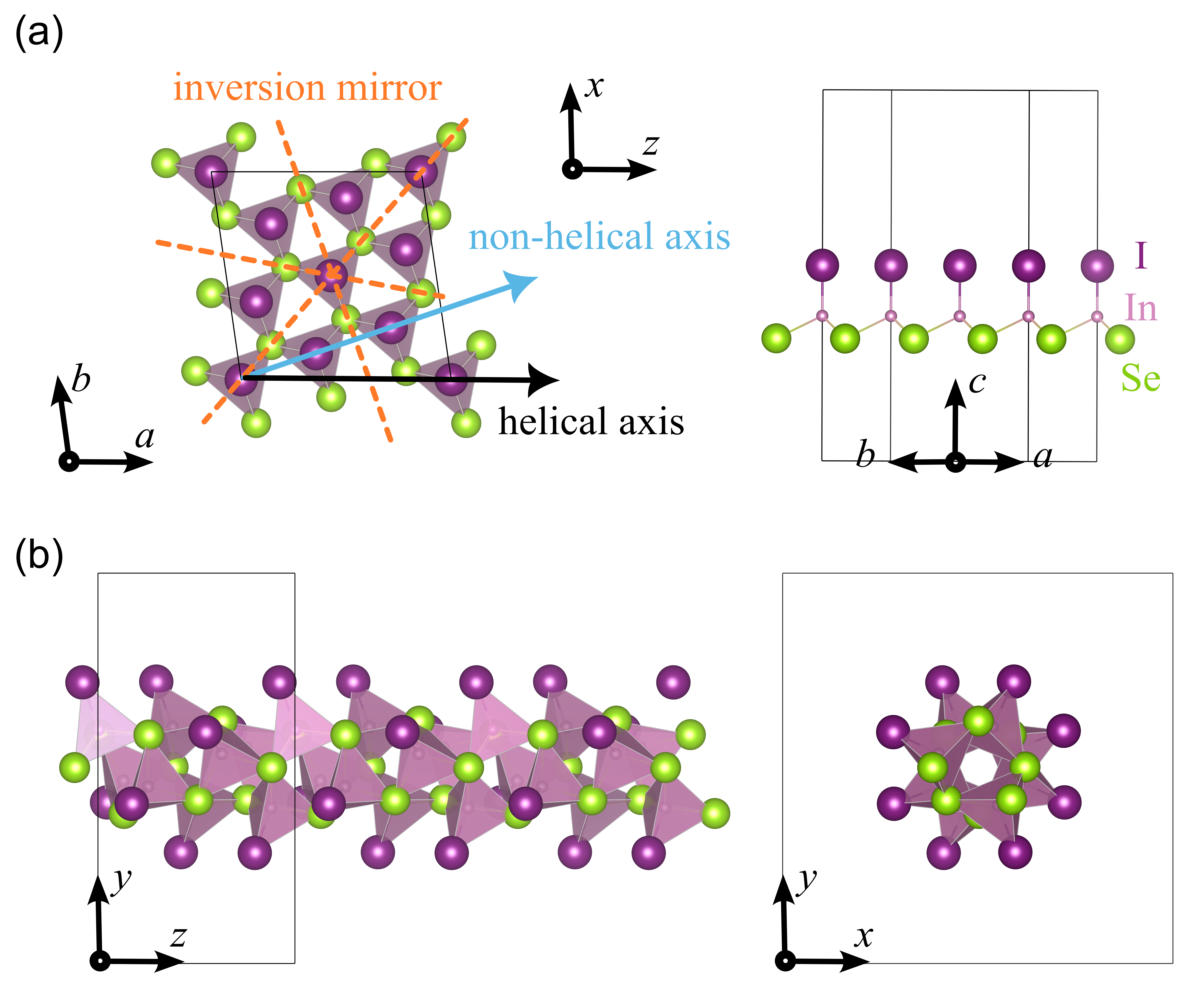
Figure 3: Planar and helical InSeI. Structure of (a) 2D planar and (b) 1D helical InSeI.

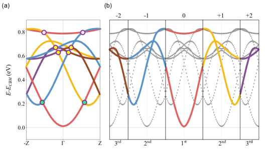
Figure 4: Electronic band structure of 1D helical InSeI in (a)crystal BZ and (b)helical BZ. Different colors are used to label different OAM quantum number $m$ which is shown at the top of (b). The red, yellow and blue bands are called band-1,2 and 3 (with $m=0,+1,-1$) respectively in following discussion. The yellow and green filled dots in (a) denote the degenerate points between bands with $m=\pm 2,m=\pm 1$ and $m=\pm 1,m=\pm 0$, which can be broken by hSOC.

To clarify the structure of helical InSeI, we first find its corresponding planar structure as shown in Fig. 3(a). By rolling along one of its unit vectors (the black arrow, the helical axis), we can construct the 1D helical InSeI as shown in Fig. 3(b). The 2D planar InSeI possesses a P3_m1 space group with three inversion mirrors (red dashed lines). Since our rolling direction is not perpendicular to any of them, the inversion symmetry along the rolling axis is broken, creating a helical structure. This can also be verified by the fact that the helical InSeI has a P4₁ space group containing a 4-fold screw axis.

The DFT-calculated energy band structure (without SOC) of helical InSeI near the conduction band minimum(CBM) is shown in Fig. 4. We focus on the conduction band (CB) rather than the valence band (VB) because the energy of the former, i.e. the electron affinity, is close to the Fermi level of commonly used metal electrodes, while the latter is not, which makes CB more practical for device manufacturing [13]. In Fig. 4(a), $k$ is defined within the first crystal BZ. As discussed in section-II.2, the atomic OAM can be inherited to the helical structure. To identify the OAM, we expand the crystal BZ to 4-times larger (from $2\pi/4a_{0}$ to $2\pi/a_{0}$) and unfold the bands continuously to obtain the helical BZ, which, as shown in Fig. 4(b), contains the first, second, third and fourth crystal BZs labelled at the panel bottom. According to the discussion in sec-II.3 about helical momentum, the parts of helical BZ that correspond to the second, third, and fourth crystal BZs are $\pm{G}$- and $\pm 2{G}$-shifted from the first crystal BZ. Therefore, the states in these parts have the corresponding helical momentum $L=\hbar(k\ {\pm}\ G)$ and $L=\hbar(k\ {\pm}\ 2G)$, with the OAM quantum number $m=\pm 1$ and $m=\pm 2$, respectively. Based on this, we can identify $m$ for the bands in the first crystal BZ, as labelled on the panel top. It can be found that the sign of $m$ is related to that of $k$, so that $L(k)=\hbar(k-mG)=-L(-k)$. This is a direct result of time-reversal symmetry, as discussed in section-II.5.

In a helical system, it is not appropriate to decompose the electronic states into globally identical spherical harmonics ($s,p_{x},p_{y}...$) as is commonly done to obtain projected density of states or bands in ab initio calculations. This is because the local chemical environment is tilted. Instead, we can directly observe the phase evolution of the wavefunction along the circumferential direction to verify the OAM. As shown in Fig. 5(a), the wavefunction of band-1 has neither a significant imaginary component nor a strong sign dependence on $\varphi$, which corresponds to a zero OAM $m=0$. In contrast, as shown in Fig. 5(b), the real and imaginary components of band-2/3 are almost identical, especially in the same significant phase variation depending on $\varphi$. The only difference is their spatial orientations, which are orthogonal to each other. By comparing with atomic orbital $p_{x},p_{y}$ in Eq. 5, which are the real and imaginary component of $p_{\pm}$ orbital (with $m=\pm 1$), respectively, we can verify that band-2/3 has a typical $|m|=1$ OAM. Besides, according to the definition of helical momentum defined in Eq. 15, band-1 in the second crystal BZ should have an OAM of $m=\pm 1$, which can also be observed, as shown in Fig. 5(c). These results strongly support the validity of our general discussion in section-II.2 II.3.

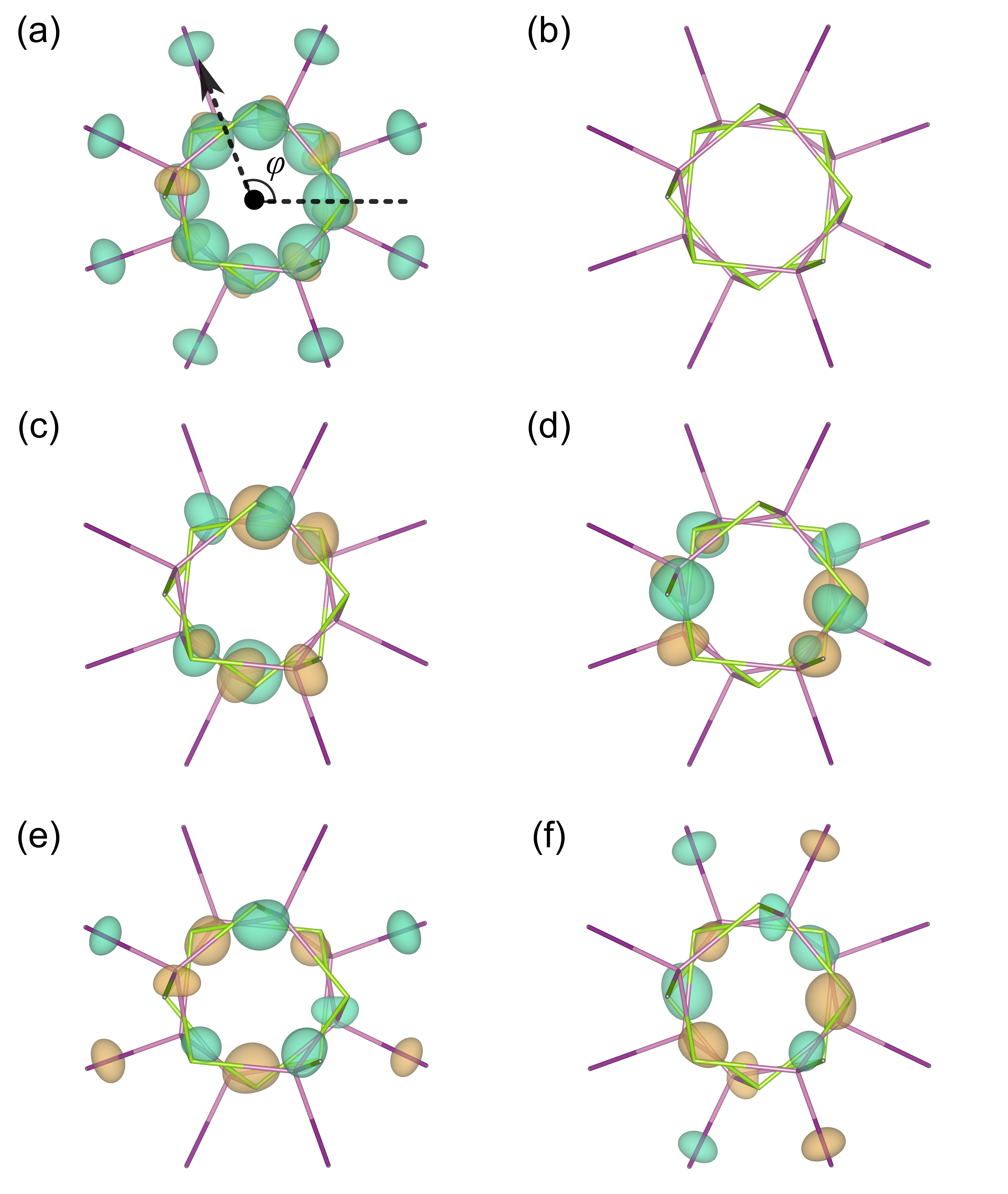
Figure 5: OAM inheritance observed in DFT results. The isosurface plot for wavefunction of (left)real and (right)imaginary part. (a) Band-1, (b) band-2 in the first BZ. (c) Band-1 in the second BZ. Only one $k$ point is arbitrarily selected but the key features are not dependent on $k$. The isosurface value is +0.12 in yellow and -0.12 in green (unit:Å${}^{-\frac{3}{2}}$).

III.2 Helical-induced SOC

Figure 6: Helical-induced SOC in InSeI. (a)DFT and (b)model band of planar InSeI. (c)DFT and (d)model band of helical InSeI. (e)DFT and (f)model band of 1D helical InSeI under 6% tensile strain. The color bar represents the expectation value of $z$-direction spin. The black and red circles highlight the spin-mixing splitting due to the hSOC. The former is not between band-1 and band-2,3 thus is beyond the description of our simplified tight-binding model while the latter can be repeated well.

With the consideration of SOC, the DFT band structures of planar InSeI and helical InSeI are shown in Fig. 6(a) and (c), respectively. Both systems have a large spin-conserving spin splitting between band-2 and band-3, which is a typical result of atomic SOC between $p_{x},p_{y}$ orbitals. However, in helical InSeI, there are spin-mixing energy gaps where the spin order becomes discontinuous. This suggests that there is an additional spin-flipping SOC only existing in helical InSeI instead of planar InSeI, which hybridizes two different spin states together. We can verify that this spin-flipping SOC is able to be well explained by our discussion about hSOC in section-III.2 from three aspects. First, according to Eq. 27, hSOC can only happen between states with ${\Delta}m=\pm 1$. As shown in Fig. 4(a), there are four degenerate points between $m=\pm 1$, $m=\pm 2$ bands (highlighted in yellow filled dots) and four degenerate points between $m=\pm 1$,$m=0$ bands (highlighted in green and white filled dots) that satisfy this restriction. The degeneracy breaking of these points coincides well with Fig. 6(a). Second, take the two low-energy degenerate points between $m=0$-band (band-1, colored in red) and $m=\pm 1$-band (band-2 and band-3, colored in blue and yellow) as highlighted in Fig. 4(b), which are broken into spin-mixing energy gaps by hSOC as highlighted in red circles in Fig. 6(c), as an example. After exerting a tensile strain $\epsilon=6\%$ to helical InSeI along the helical axis, as is shown in Fig. 6(e), the gaps still exist but are significantly reduced. This can be explained by the fact that the tensile strain descends the energy of band-2/3 relative to band-1, so the two spin-mixing gaps are shifted towards the $\Gamma$ point and their $|k|$ value is reduced. According to Eq. 27, which states that $H_{SO}$ is proportional to $k$, the strength of the spin-flipping SOC should be negatively related to the tensile strain, which is in agreement with the DFT results.

Finally, as a more detailed verification, we build a low-energy-effective tight-binding model for band-1,2,3 based on the discussion in section-II.2 and II.3. There are three basis states: two $p_{x},p_{y}$-type ($|m|=1$) denoted as $|x{\rangle},|y{\rangle}$, and one $s$-type ($|m|=0$) denoted as $|z{\rangle}$, each with two spin components, for a total six bands in this model (details can be found in section-A.1). Roughly fitting our model to the DFT band structure, we can see in Fig. 6(d) that our model is able to give successful interpretation to the dispersion, parity, spin texture, and spin splitting for 1D helical InSeI. Therefore, it can be concluded that our analysis about helical-induced SOC works well in explaining DFT results, which proves the validity of our corresponding discussion in sec-II.

Figure 7: Helical-induced polarization of helical InSeI. (a) Ballistic conductance and spin polarization arising from hSOC in helical InSeI. The spin-conserving and spin-flipping conductances are polarized as $G_{\uparrow{\uparrow}}>G_{\downarrow{\downarrow}}$ and $G_{\uparrow{\downarrow}}{\neq}G_{\downarrow{\uparrow}}$, a non-zero spin polarization $P$ can be achieved. If the hSOC turned off, $G_{\uparrow{\uparrow}}=G_{\downarrow{\downarrow}}$ and $G_{\uparrow{\downarrow}}=G_{\downarrow{\uparrow}}=0$, leading to a zero polarization. (b) Chirality dependent shift current conductivity $\sigma^{zzz}$ induced by non-zero Berry connection in helical InSeI.

Helical InSeI is a promising material for spintronic devices based on the spin-flipping hSOC. Consider an InSeI nanowire with a length of 80 unitcells. If we connect this nanowire to two electrodes and apply a small bias voltage ${\Delta}V$, we can create an electric current that flows through the nanowire. According to the Landauer-Buttiker formalism for ballistic transport [21], the electric current can be calculated as

$$I =\frac{1}{e}\int_{E_{f}-{\Delta}V}^{E_{f}+{\Delta}V}G(E)[f_{1}(E)-f_{2}(E)]dE$$ (30)

$${\approx}\ G(E_{f}){\Delta}V/e$$

where $G(E)$ is the conductance contributed by the electronic states with energy $E$ and $f_{1,2}(E)$ is the Fermi-Dirac distribution function in electrode 1,2. The approximate equality is valid for small ${\Delta}V$, so the current is simply proportional to $G(E_{f}){\equiv}G$, which means that only the states near $E_{f}$ contribute to conduction. The conductance for spin-up/down electrons moving from one electrode to another without changing their spin states is denoted by $G_{{\uparrow}{\uparrow}}$/$G_{{\downarrow}{\downarrow}}$, which is called the spin-conserved conductance. Similarly, the spin-flipping conductance is denoted by $G_{{\downarrow}{\uparrow}},G_{{\uparrow}{\downarrow}}$. To characterize the spin selectivity, we also define the spin polarization of electronic current as

$$P =\frac{I_{{\uparrow}{\uparrow}}+I_{{\downarrow}{\uparrow}}-I_{{\downarrow}{\downarrow}}-I_{{\uparrow}{\downarrow}}}{I_{{\uparrow}{\uparrow}}+I_{{\downarrow}{\uparrow}}+I_{{\downarrow}{\downarrow}}+I_{{\uparrow}{\downarrow}}}$$ (31)

$${\sim}\frac{G_{{\uparrow}{\uparrow}}+G_{{\downarrow}{\uparrow}}-G_{{\downarrow}{\downarrow}}-G_{{\uparrow}{\downarrow}}}{G_{{\uparrow}{\uparrow}}+G_{{\downarrow}{\uparrow}}+G_{{\downarrow}{\downarrow}}+G_{{\uparrow}{\downarrow}}}$$

If $P>0$($P<0$) the spin-up(down) current is larger, or in other words, the spin-up (down) conductance is larger, so that the current carries net spin. Otherwise, the current is spin degenerate.

Based on the tight-binding model built in section-A.1, we calculate the $G$ and $P$ for InSeI under 6% tensile strain (in order to lower down the spin-splitting region of band-2/3). As shown in Fig. 7(a), both the spin-conserved and spin-flipping conductance are polarized, which generates a spin-polarized current. The polarization peak is achieved with $E_{f}-E_{CBM}$ around 0.1-0.125 eV, where $E_{f}$ is roughly located around the middle of the spin-splitting energy gap of band-2/3, as can be seen in Fig. 6(e)(f). All these spin-polarization vanishes if we turn off the hSOC, even though the intrinsic atomic SOC is still on and the spin-conserving spin-splitting energy gap between band-2/3 still exists. Therefore, it is the hSOC that activates the spin-splitting band in helical InSeI to create the spin-polarized response to a static electric field.

Additionally, since hSOC is a purely imaginary off-diagonal term in the Hamiltonian, even though its sign changes when the chirality is reversed, as shown in Eq. 27, its effect on eigen-energies remains the same. Therefore, the spin-selectivity will be reversed for opposite chirality because changing chirality will reverse the $z$-direction spin from spin-up/down to spin-down/up. To be more specific, if left-handed helical InSeI has a higher spin-up conductivity, then the right-handed InSeI should have a higher spin-down conductivity, which can be used to distinguish chirality of helical InSeI or degisn spintronic devices with different spin-selectivity.

III.3 Helical-induced shift current

A non-zero Berry phase in helical InSeI can be characterized by the DFT-calculated polarization $\pm 3.098$ eÅ with opposite signs for different chiralities. This results in a shift current under a linearly polarized monochromatic electric field $\bm{E}(t)=\bm{E}(\omega)e^{-i\omega t}+c.c.$, denoted by $j_{\operatorname{sc}}^{a}=2\sigma^{abb}(0;\omega,-\omega)\operatorname{Re}\left[E_{b}(\omega)E_{b}(-\omega)\right]$, which is a second-order nonlinear photocurrent response that flows along the helical axis in opposite directions for different chiralities. The conductivity is given by [22, 23]

$$\sigma^{abb}(0;\omega,-\omega) =-\frac{\pi e^{3}}{\hbar^{2}}\int\frac{d\bm{k}}{(2\pi)^{d}}\sum_{nm}f_{nm}R_{mn}^{a,b}r_{nm}^{b}r_{nm}^{b}$$ (32)

$$\times\delta\left(\omega_{nm}-\omega\right).$$

Here, $f_{nm}=f_{n}-f_{m}$ and $\hbar\omega_{nm}=\varepsilon_{n}-\varepsilon_{m}$ denote the difference in occupation numbers and energies between bands $n$ and $m$, respectively. $d$ is the dimension. $r_{nm}^{b}=i\left\langle u_{\bm{k}n}\mid\partial_{b}u_{\bm{k}m}\right\rangle$ and $\mathcal{A}_{n}^{b}=i\left\langle u_{\bm{k}n}\mid\partial_{b}u_{\bm{k}n}\right\rangle$ are the interband and intraband Berry connections. $R_{mn}^{a,b}(\bm{k})=-\partial_{a}\arg r_{mn}^{b}(\bm{k})+\mathcal{A}_{m}^{a}(\bm{k})-\mathcal{A}_{n}^{a}(\bm{k})$ is the gauge invariant shift vector. It is clear from this expression that the shift vector is proportional to the difference in Berry connections. Therefore, reversing the chirality in helical InSeI will reverse the shift current along the helical axis.

To calculate the conductivity $\sigma$, we first constructed quasiatomic Wannier functions and a first-principles tight-binding Hamiltonian from Kohn–Sham wavefunctions and eigenvalues, using the maximal similarity measure with respect to pseudoatomic orbitals. This yielded 192 quasiatomic Wannier functions, which consist of combinations of $s$ and $p$ orbitals derived from In, Se, and I atoms. We then used the developed tight-binding Hamiltonian to compute the nonlinear shift current, using a dense k-point sampling of 1 $\times$ 1 $\times$ 100. A small imaginary smearing factor of $\eta$ = 0.025 eV was used for the Dirac delta function integration. The calculated $\sigma$ is shown in Fig. 7(b), where a clear sign change for different chiralities is observed. This result not only agrees with our discussion in section-II.4 but also proves that the shift current is an effective way to detect chirality.

IV Conclusions

In this paper, we investigated the electronic states in helical systems and verified our findings using DFT calculations. Our investigation has revealed several distinctive properties inherent to helical systems. Firstly, helical structures can inherit the atomic OAM of their constituent atoms. Secondly, the conserved quantity in helical systems with screw symmetry is the helical momentum, which is composed of both crystal momentum and OAM. Thirdly, the helically arranged atoms create a helical potential that induces spin-flipping SOC. The inherent chirality of the helical structure enables chiral-switchable Berry phase, which leads to opposite shift current responses in helical InSeI with different chiralities. These properties suggest that helical systems have rich potential for applications in spintronics, optoelectronics, and beyond. Our work is expected to shed light on further exploration of the distinctive properties and versatile applications of helical systems.

Appendix A Appendix

A.1 Details of tight-binding modeling

As is defined in section-III.1, $|x{\rangle}$ and $|y{\rangle}$ are $p_{x},p_{y}$-type with the orbital angular momentum component $m=\pm 1$.

$$|x{\rangle} =\frac{1}{\sqrt{2}}(|-1{\rangle}-|1{\rangle})$$ (33)

$$|y{\rangle} =\frac{i}{\sqrt{2}}(|-1{\rangle}+|1{\rangle})$$

InSeI has a 4-fold screw symmetry ($\zeta=4$), so that the directional polarization difference between two adjenct helical sites as is discussed in section-II.2 becomes ${\Delta}\varphi=2\pi/4=\pi/2$. According to Eq. 14, we have

$${\langle}+1|H|+1{\rangle}$$ (34)

$$=\frac{t_{1}}{2}(e^{i\pi/2}e^{ika}+e^{-i\pi/2}e^{-ika})$$

$$=\frac{t_{1}}{2}(ie^{ika}-ie^{-ika})$$

$$=t_{1}\sin(ka)$$

$$=-{\langle}-1|H|-1{\rangle}$$

where $t_{1}$ is the Slater-Koster coefficient. Within the first BZ, hopping is forbidden for ${\Delta}l\neq 0$ so that

$${\langle}\pm 1|H|\mp 1{\rangle}=0$$ (35)

Therefore the hopping paramter between $|x{\rangle}$ and $|y{\rangle}$ can be calculated as

$$h_{xy} ={\langle}x|H|y{\rangle}$$ (36)

$$=\frac{i}{2}({\langle}-1|-{\langle}+1|)H(|-1{\rangle}+|+1{\rangle})$$

$$=i\frac{{\langle}-1|H|-1{\rangle}-{\langle}+1|H|+1{\rangle}}{2}$$

$$=it_{1}\sin(ka)$$

$$h_{xx} ={\langle}x|H|x{\rangle}$$ (37)

$$=\frac{1}{2}({\langle}-1|-{\langle}+1|)H(|-1{\rangle}-|+1{\rangle})$$

$$=\frac{{\langle}-1|H|-1{\rangle}+{\langle}+1|H|+1{\rangle}}{2}$$

$$=0=h_{yy}$$

Recall that $|x{\rangle}$ and $|y{\rangle}$ are directional polarized to global $x$- and $y$-direction respectively. Therefore the tight-binding Hamiltonian of $(|x{\rangle},|y{\rangle})^{\pmb{T}}$ subspace ${H_{xy}}$ should satisfy the 4-fold rotational symmetry, or in other words, be invariant under 90^∘-rotational operation along ${z}$-axis as

$$H_{xy} =\begin{bmatrix}h_{xx}&h_{xy}\\ h_{xy}^{*}&h_{yy}\end{bmatrix}$$ (38)

$$=R^{-1}H_{xy}R$$

$$=\begin{bmatrix}0&-1\\ 1&0\end{bmatrix}\begin{bmatrix}h_{xx}&h_{xy}\\ h_{xy}^{*}&h_{yy}\end{bmatrix}\begin{bmatrix}0&1\\ -1&0\end{bmatrix}$$

$$=\begin{bmatrix}h_{yy}&-h_{xy}^{*}\\ -h_{xy}&h_{xx}\end{bmatrix}$$

$${\Rightarrow}h_{xx}=h_{yy},\ \ \text{Re}[V_{xy}]=0$$

and Eq. 36,37 agrees well with this requirement. Since $|z{\rangle}$ has no OAM $m=0$ thus its self hopping is simply

$$h_{zz}={\langle}z|H|z{\rangle}=\frac{t_{2}}{2}(e^{ika}+e^{-ika})=t_{2}\cos(ka)$$ (39)

and also has no hopping with $|x{\rangle},|y{\rangle}$ due to the non-zero ${\Delta}l$.

According to Eq. 27, the angular momentum conservation requires that hSOC is only non-zero for $|{\Delta}m|=1$, thus ${\langle}\pm 1|\hat{H}_{SO}|\pm 1{\rangle}=0$ so that ${\langle}x|\hat{H}_{SO}|y{\rangle}={\langle}y|\hat{H}_{SO}|x{\rangle}=0$. The only non-zero term is between $|x,y{\rangle}$ and $|z{\rangle}$ as

$${\langle}x|\hat{H}_{SO}|z{\rangle} =\frac{1}{\sqrt{2}}({\langle}-1|\hat{H}_{SO}|0{\rangle}-{\langle}+1|\hat{H}_{SO}|0{\rangle})$$ (40)

$$=\lambda_{R}({\sigma}_{+}-{\sigma}_{-})$$

$$=i\lambda_{R}{\sigma_{y}}$$

$${\langle}y|\hat{H}_{SO}|z{\rangle} =\frac{i}{\sqrt{2}}({\langle}-1|\hat{H}_{SO}|0{\rangle}+{\langle}+1|\hat{H}_{SO}|0{\rangle})$$ (41)

$$=i\lambda_{R}({\sigma}_{+}+{\sigma}_{-})$$

$$=i\lambda_{R}{\sigma_{x}}$$

where the relation between $\sigma_{x,y}$ and $\sigma_{\pm}$ is obtained from Eq. 25. The strength of hSOC is denoted as $\lambda_{R}$. Besides, there is also an intrinsic atomic SOC between $|x{\rangle},|y{\rangle}$ with the form $\lambda_{0}\sigma_{z}$ which is irrelevant to the helical structure [24].

Based on all the above analysis, the tight-binding model with the basis

$$(|x_{\uparrow}{\rangle},|y_{\uparrow}{\rangle},|z_{\uparrow}{\rangle},|x_{\downarrow}{\rangle},|y_{\downarrow}{\rangle},|z_{\downarrow}{\rangle})^{\textbf{T}}$$

is finally obtained as

$$H=\begin{bmatrix}H_{{\uparrow}{\uparrow}}&H_{{\uparrow}{\downarrow}}\\ H_{{\downarrow}{\uparrow}}&H_{{\downarrow}{\downarrow}}\end{bmatrix}$$ (42)

$$H_{{\uparrow}{\uparrow}}=\begin{bmatrix}U_{1}&it_{1}\sin(ka)+i{\lambda_{0}}&0\\ {\dagger}&U_{1}&0\\ {\dagger}&{\dagger}&U_{2}+t_{2}\cos(ka)\end{bmatrix}$$ (43)

$$H_{{\downarrow}{\downarrow}}=\begin{bmatrix}U_{1}&it_{1}\sin(ka)-i{\lambda_{0}}&0\\ {\dagger}&U_{1}&0\\ {\dagger}&{\dagger}&U_{2}+t_{2}\cos(ka)\end{bmatrix}$$ (44)

$$H_{{\uparrow}{\downarrow}}=\begin{bmatrix}0&0&{\lambda_{R}}\\ 0&0&i{\lambda_{R}}\\ -{\lambda_{R}}&-i{\lambda_{R}}&0\end{bmatrix}$$ (45)

$$H_{{\uparrow}{\downarrow}}=H_{{\downarrow}{\uparrow}}^{\dagger}$$ (46)

where ${\lambda_{R}}={\lambda_{R0}}ka$. Roughly fitting tight-binding band to DFT results, we have $\lambda_{0}=-0.06,\lambda_{R0}=0.45\lambda_{0},U_{1}=0.5,U_{2}=U_{1}-0.15$. For equilibrium InSeI $t_{1}=-0.3,t_{2}=-0.35$ and for 6% tensile strain InSeI $t_{1}=-0.425,t_{2}=-0.25$ (with unit eV).

A.2 Quantum ballistic transport

Through retarded Green’s function $G^{R}$ and transmissian matrix $\bar{T}$ we could obtain ballistic conductance $G(E)$

$$G(E)=G_{0}\bar{T}(E)$$

$$\bar{T}(E)={\rm Tr}[{\Gamma_{1}}G^{R}{\Gamma_{2}}G^{R,\dagger}]$$

$${\Gamma_{1,2}}=i[{\Sigma_{1,2}}-{\Sigma_{1,2}^{\dagger}}]=-2{\rm Im}\{\Sigma_{1,2}\}$$

$$G^{R}=[E-H_{C}-{\Sigma_{1}}-{\Sigma_{2}}]^{-1}$$

where $G_{0}=2e^{2}/\hbar$ is conductance quantum and $\Sigma_{1,2}$ is the 1,2 electrode self-energy. Approximately if only consider one conducting state with two spin components for each electrode we obtain

$${\Sigma_{1,2;{\uparrow},{\downarrow}}}={\omega}\exp(i\pi\sqrt{\frac{E-E_{0}}{E_{k}}})$$ (47)

where $\omega$ is in energy unit and represents the strength of electrode-InSeI coupling, $E_{k}={\hbar}^{2}{\pi}^{2}/2ma^{2}$ is the characteristic kinetic energy of electrons in electrode with potential energy shift $E_{0}$. Without losing any generality we select $\omega=-0.8$ eV, $E_{k}=1.5$ eV and $E_{0}=-1.0$ eV (reference to InSeI CBM). Use equ-43-46 we obtain an N-unitcell sample Hamiltonian $H_{C}$ as

$$H_{C}=\begin{bmatrix}H_{0}&T&0&0&0&...\\ T^{\dagger}&H_{1}&T&0&0&...\\ 0&T^{\dagger}&H_{2}&T&0&...\\ &&...\end{bmatrix}_{N{\times}N}$$ (48)

$$H_{n}=\begin{bmatrix}h_{n,{\uparrow}{\uparrow}}&h_{{\uparrow}{\downarrow}}\\ h_{{\downarrow}{\uparrow}}&h_{n,{\downarrow}{\downarrow}}\end{bmatrix}$$

$$h_{n,{\uparrow}{\uparrow}}=\begin{bmatrix}U_{xx}+n{\Delta}{\phi}&i{\lambda_{0}}&0\\ {\dagger}&U_{yy}+n{\Delta}{\phi}&0\\ {\dagger}&{\dagger}&U_{zz}+n{\Delta}{\phi}\end{bmatrix}$$

$$h_{n,{\downarrow}{\downarrow}}=\begin{bmatrix}U_{xx}+n{\Delta}{\phi}&-i{\lambda_{0}}&0\\ {\dagger}&U_{yy}+n{\Delta}{\phi}&0\\ {\dagger}&{\dagger}&U_{zz}+n{\Delta}{\phi}\end{bmatrix}$$

$$h_{{\uparrow}{\downarrow}}=\begin{bmatrix}0&0&{\lambda_{R}}\\ 0&0&i{\lambda_{R}}\\ -{\lambda_{R}}&-i{\lambda_{R}}&0\end{bmatrix}$$

$$T=\begin{bmatrix}t_{{\uparrow}{\uparrow}}&0\\ 0&t_{{\downarrow}{\downarrow}}\end{bmatrix}$$

$$t_{{\uparrow}{\uparrow}}=t_{{\downarrow}{\downarrow}}=\begin{bmatrix}0&iV_{sp}&0\\ -iV_{sp}&0&0\\ 0&0&V_{pp}\end{bmatrix}$$

where ${\Delta}\phi={\Delta}V/N$ is the electrochemical potential bias per unitcell.

A.3 Classical spin-selective transport

We regard the total electrostatic potential energy of an electron, $U$, as if it were due to an effective point charge in the distance $r$, such that $U=eV=eK/r=e|E|r$, where $|E|=K/r^{2}$ is the effective electric field intensity. Due to the chirality of the helix structure, any drifting motion of electron along $z$-direction will be accompanied by a rotating field $E$, which means $E$ is time-dependent in the rest reference system of the electron. According to the Maxwell equation, this will induce a magnetic field $H$ as

$${\nabla}{\times}\vec{H}={\epsilon}{\partial}_{t}\vec{E}$$ (49)

or in the integral form

$${\int}_{\Omega}{\nabla}{\times}\vec{H}{\cdot}d\vec{S}={\int}_{{\partial}{\Omega}}\vec{H}{\cdot}d\vec{l}={\int}_{\Omega}({\mu}{\epsilon}){\partial}_{t}\vec{E}{\cdot}d\vec{S}$$

Let $\Omega$ be a rectangular region with length $dz$ in the $z$-direction and width $r$ in radius direction(${\perp}z$-direction). Then, we obtain

$$H_{z}dz=(\pm){\epsilon}|E|{\omega_{e}}rdz$$ (50)

where $\pm$ denotes the electron moving direction ${\pm}z$. Here, we assume that the rotating radius $r$ and the rotation angular frequency $\omega_{e}$ are constant (i.e. the rotation is circular), considering that each In-Se-I tetrahedra has the same structure. With the helix spatial period $a_{0}$ and electron velocity $v_{z}$, we have $\omega_{e}=2{\pi}/T=2{\pi}/(a_{0}/v_{z})$. Considering $v_{z}$ is caused by external electric field $E_{z}$, we obtain $v_{z}=ME_{z}$, where $M$ is the mobility. Plugging these relations into equ-50, we have the magnetic induction intensity $B_{z}={H_{z}/{\mu}}$ and

$$|B_{z}|=\frac{\epsilon_{r}}{ec^{2}}{\omega_{e}}U=(\frac{1}{ec^{2}})(\frac{{\epsilon_{r}}UM}{a_{0}})E_{z}$$

In the indirect-gap phase, the $+k$ and $-k$ CBMs have opposite $z$-direction spin, thus a Zeeman energy splitting near CBM is created between spins as

$${\Delta}E_{B}=2{\mu_{B}}B_{z}=(\frac{{\hbar}}{m_{e}c^{2}})\frac{{\epsilon_{r}}MU}{a_{0}}E_{z}$$ (51)

where $\mu_{B}=e\hbar/2m_{e}$ is Bohr magneton. Consequently, the spin-up/down carrier density will be different, leading to a spin-polarized current

$$P {\equiv}\frac{I_{\uparrow}-I_{\downarrow}}{I_{\uparrow}+I_{\downarrow}}=\frac{n_{\uparrow}-n_{\downarrow}}{n_{\uparrow}+n_{\downarrow}}$$ (52)

$$=\frac{1-\exp(-\frac{{\Delta}E_{B}}{kT})}{1+\exp(-\frac{{\Delta}E_{B}}{kT})}=\tanh(\frac{{\Delta}E_{B}}{2kT})$$

$$=\tanh(E_{z}/E_{z0})$$

via characteristic electric field intensity $E_{z0}$ as

$$E_{z0}=(\frac{kT}{U})(\frac{m^{*}c^{2}}{\hbar})\frac{a_{0}}{{\epsilon_{r}}M}$$ (53)

As an estimation, with room temperature $kT=0.026$ eV, total electrostatic potential $U\ {\sim}\ 15$ eV, $m_{e}c^{2}/\hbar=1.2{\times}10^{20}$ 1/s, $M=5.42{\times}10^{-3}{\rm m^{2}/(V{\cdot}s)}$, $a_{0}=30.0$Å, ${\epsilon_{r}}{\sim}5$, the characteristic $E_{z0}{\sim}10^{10}\ {\rm V/m}$, which is around the order of magnitude of electric field intensity inside atom. Therefore, commonly a linear approximation is safe enough to be adopted as

$$P\ {\sim}\ E_{z}/E_{z0}$$

It can be concluded that low temperature and strong external electric field are necessary conditions for observing a significant spin polarization. Any improvement to electron carrier mobility is also beneficial.

References

- Yang et al. [2021] S.-H. Yang, R. Naaman, Y. Paltiel, and S. S. Parkin, Nature Reviews Physics 3, 328 (2021).
- Naaman and Waldeck [2012] R. Naaman and D. H. Waldeck, The Journal of Physical Chemistry Letters 3, 2178 (2012).
- Gutierrez et al. [2012] R. Gutierrez, E. Díaz, R. Naaman, and G. Cuniberti, Physical Review B 85, 081404 (2012).
- Guo and Sun [2012] A.-M. Guo and Q.-f. Sun, Physical Review Letters 108, 218102 (2012).
- Varela et al. [2016] S. Varela, V. Mujica, and E. Medina, Physical Review B 93, 155436 (2016).
- Medina et al. [2012] E. Medina, F. López, M. A. Ratner, and V. Mujica, Europhysics Letters 99, 17006 (2012).
- Liu et al. [2021] Y. Liu, J. Xiao, J. Koo, and B. Yan, Nature Materials 20, 638 (2021).
- Hu et al. [2018] L. Hu, H. Huang, Z. Wang, W. Jiang, X. Ni, Y. Zhou, V. Zielasek, M. Lagally, B. Huang, and F. Liu, Physical Review Letters 121, 066401 (2018).
- Yang and Kotov [2011] M. Yang and N. A. Kotov, Journal of Materials Chemistry 21, 6775 (2011).
- Pfister et al. [2016] D. Pfister, K. Schäfer, C. Ott, B. Gerke, R. Pöttgen, O. Janka, M. Baumgartner, A. Efimova, A. Hohmann, P. Schmidt, et al., Advanced Materials 28, 9783 (2016).
- Ivanov et al. [2012] A. S. Ivanov, A. J. Morris, K. V. Bozhenko, C. J. Pickard, and A. I. Boldyrev, Angewandte Chemie-International Edition 51, 8330 (2012).
- Jiang et al. [2020] S. Jiang, H. Yin, G.-P. Zheng, B. Wang, S. Guan, and B.-J. Yao, Physical Chemistry Chemical Physics 22, 27441 (2020).
- Zhao et al. [2023] S. Zhao, J. Hu, Z. Zhu, X. Yao, and W. Li, Chirality-induced Spin Splitting in 1D InSeI (2023), arXiv:2308.04350 [cond-mat.mtrl-sci] .
- Choi et al. [2022] K. H. Choi, S. Cho, B. J. Jeong, B. Lee, J. Jeon, J. Kang, X. Zhang, H.-S. Oh, J.-H. Lee, H. K. Yu, et al., Journal of Alloys and Compounds 927, 166995 (2022).
- Kaxiras [2003] E. Kaxiras, Atomic and Electronic Structure of Solids (Cambridge University Press, 2003).
- Marzari and Vanderbilt [1997] N. Marzari and D. Vanderbilt, Physical Review B 56, 12847 (1997).
- Atkins and Friedman [2011] P. W. Atkins and R. S. Friedman, Molecular Quantum Mechanics (Oxford University Press, 2011).
- Božovic [1984] I. Božovic, Physical Review B 29, 6586 (1984).
- Kittel et al. [1996] C. Kittel, P. McEuen, and P. McEuen, Introduction to Solid State Physics, Vol. 8 (Wiley New York, 1996).
- Manchon et al. [2015] A. Manchon, H. C. Koo, J. Nitta, S. M. Frolov, and R. A. Duine, Nature Materials 14, 871 (2015).
- Datta [1997] S. Datta, Electronic Transport in Mesoscopic Systems (Cambridge University Press, 1997).
- Sipe and Shkrebtii [2000] J. Sipe and A. Shkrebtii, Physical Review B 61, 5337 (2000).
- Wang et al. [2022] H. Wang, X. Tang, H. Xu, J. Li, and X. Qian, npj Quantum Materials 7, 61 (2022).
- Dai et al. [2008] D. Dai, H. Xiang, and M.-H. Whangbo, Journal of Computational Chemistry 29, 2187 (2008).
- Kishine [2023] J. Kishine, JPSJ News and Comments 20, 03 (2023).