Leveraging hierarchical feature sharing for efficient dataset condensation

Abstract

Given a real-world dataset, data condensation (DC) aims to synthesize a significantly smaller dataset that captures the knowledge of this dataset for model training with high performance. Recent works propose to enhance DC with data parameterization, which condenses data into parameterized data containers rather than pixel space. The intuition behind data parameterization is to encode shared features of images to avoid additional storage costs. In this paper, we recognize that images share common features in a hierarchical way due to the inherent hierarchical structure of the classification system, which is overlooked by current data parameterization methods. To better align DC with this hierarchical nature and encourage more efficient information sharing inside data containers, we propose a novel data parameterization architecture, Hierarchical Memory Network (HMN). HMN stores condensed data in a three-tier structure, representing the dataset-level, class-level, and instance-level features. Another helpful property of the hierarchical architecture is that HMN naturally ensures good independence among images despite achieving information sharing. This enables instance-level pruning for HMN to reduce redundant information, thereby further minimizing redundancy and enhancing performance. We evaluate HMN on four public datasets (SVHN, CIFAR10, CIFAR100, and Tiny-ImageNet) and compare HMN with eight DC baselines. The evaluation results show that our proposed method outperforms all baselines, even when trained with a batch-based loss consuming less GPU memory.

1 Introduction

Data condensation (DC) Wang et al. (2018), also known as data distillation, has emerged as a valuable technique for compute-efficient deep learning Bartoldson et al. (2023); Zheng et al. (2020). It aims to synthesize a much smaller dataset while maintaining a comparable model performance to the case with full dataset training. Data condensation offers advantages in various applications, such as continual learning Rosasco et al. (2022); Sangermano et al. (2022), network architecture search Zhao & Bilen (2023b), and federated learningSong et al. (2022); Xiong et al. (2022). Because of the considerable practical utility of data condensation, substantial efforts Du et al. (2022); Nguyen et al. (2021; 2020); Shin et al. (2023); Cui et al. (2023) have been invested in improving its efficacy. Among them, data parameterization Liu et al. (2022); Kim et al. (2022) has been proposed, which condenses data into parameterized data containers instead of the pixel space. Those data parameterization methods usually generate more images given the same storage budget and improve data condensation performance. The intuition behind data parameterization methods is to encode shared features among images together to avoid additional storage costs.

Recognizing this shared feature insight, it’s important to delve deeper into the inherent structure of these shared features in datasets. We notice that images share common features in a hierarchical way due to the inherent hierarchical structure of the classification system. Even if images differ in content, they can still share features at different hierarchical levels. For example, two images of cats can share common features specific to the cat class, but an image of a cat and another of a dog may still have shared features of the broader animal class. However, current data parameterization methods that adopt factorization to share features among images overlook this hierarchical nature of shared features in datasets. In this paper, to better align with this hierarchical nature and encourage more efficient information sharing inside data containers, we propose a novel data parameterization architecture, Hierarchical Memory Network (HMN). As illustrated in Figure 1, an HMN comprises a three-tier memory structure: dataset-level memory, class-level memory, and instance-level memory. Examples generated by HMNs share information via common dataset-level and class-level memories.

Another helpful property of the hierarchical architecture is that HMN naturally ensures good independence among images. We find that condensed datasets contain redundant data, indicating room for further improvement in data condensation by pruning redundant data. However, pruning redundant images for current data parameterization methods is challenging, since methods like HaBa Liu et al. (2022) and LinBa Deng & Russakovsky (2022) adopt factorization to achieve information sharing among images. Factorization leads to weights in data containers associated with multiple training images, which causes difficulty in pruning a specific image. Different from factorization-based methods, HMN naturally ensures better independence among images. Even though images generated by HMN share dataset-level and class-level memories, each generated image has its own instance-level memory. Thus, pruning redundant images to achieve better data efficiency can easily be done by pruning corresponding instance-level memories. We take advantage of this property of HMNs by first condensing a given dataset to a slightly over-budget HMN and then pruning the instance-level memories of redundant images to get back within allocated budgets.

We evaluate our proposed methods on four public datasets (SVHN, CIFAR10, CIFAR100, and Tiny-ImageNet) and compare HMN with the other eight baselines. The evaluation results show that, even when trained with a low GPU memory consumption batch-based loss, HMN still outperforms all baselines, including those using high GPU memory trajectory-based losses. As far as we know, HMN is the first method to achieve such good performance with a low GPU memory loss. We believe that HMN provides a strong baseline for exploring data condensation with limited GPU memory. For a fair comparison, we also compare HMN with other data parameterization baselines under the same loss. We find that HMN outperforms these baselines by a larger margin. For instance, HMN outperforms at least 3.7%/5.9%/2.4% than other data parameterization methods within 1/10/50IPC storage budgets when trained with the same loss on CIFAR10, respectively. Additionally, we also apply HMN to continual learning tasks. The evaluation results show that HMNs effectively improve the performance on continual learning.

To summarize, our contributions are as follows:

1. We propose a novel data parameterization method, Hierarchical Memory Network (HMN), comprising a three-tier memory structure: dataset-level, class-level, and instance-level.

2. We show that redundant data exist in condensed datasets. HMN inherently ensures good independence for generated images, facilitating the pruning of redundant images. We propose a pruning algorithm to reduce redundant information in HMNs.

3. We evaluate the performance of HMN on four public data and show that HMN outperforms eight SOTA baselines, even when we train HMNs with a batch-based loss consuming less GPU memory. We also compare HMN with other data parameterization baselines under the same loss. We find that HMN outperforms baselines by a larger margin.

2 Related Work

There are two main lines of approaches for improving data condensation: 1) designing better training losses and 2) increasing representation capability by data parameterization:

Training losses for data condensation. The underlying principle of data condensation is to optimize the synthetic dataset to exhibit a similar training behavior as the original dataset. There are two main types of training loss that are used to optimize synthetic datasets: 1) trajectory-based loss Wang et al. (2018); Cazenavette et al. (2022), and 2) batch-based loss Zhao & Bilen (2023b; 2021). Condensing using trajectory loss requires training the model on the synthetic dataset for multiple iterations while monitoring how the synthetic dataset updates the model parameters across iterations. For instance, MTT Cazenavette et al. (2022) employs the distance between model parameters of models trained on the synthetic dataset and those trained on the original dataset as the loss metric. In contrast, batch-based loss aims to minimize the difference between a batch of synthetic data and a batch of original data. Gradient matching Zhao et al. (2021); Lee et al. (2022); Jiang et al. (2022) calculates the distance between the gradients of a batch of condensed data and original data, while distribution matching Zhao & Bilen (2023b) computes the distance between the embeddings of a batch of real data and original data. Since trajectory-based losses keep track of the long-term training behavior of synthetic datasets, trajectory-based losses generally show better empirical performance than batch-based losses. However, trajectory-based losses have considerably larger GPU memory consumption, potentially leading to scalability issues Cazenavette et al. (2022); Cui et al. (2022). In this paper, we show that, equipped with HMN, a batch-based loss can also achieve comparable and even better performance than methods based on trajectory-based loss.

Data parameterization for data condensation. Apart from training loss, data parameterization has been recently proposed as another approach to improve data condensation. Instead of utilizing independent images as data containers, recent works Deng & Russakovsky (2022); Liu et al. (2022); Kim et al. (2022) propose to use free parameters to store the condensed information. Those data parameterization methods usually generate more images given the same storage budget and improve data condensation performance by sharing information across different examples. HaBa Liu et al. (2022) and LinBa Deng & Russakovsky (2022) concurrently introduced factorization-based data containers to improve data condensation by sharing common information among images.

Some recent work Cazenavette et al. (2023); Zhao & Bilen (2022) explores generating condensed datasets with generative priors Brock et al. (2017); Chai et al. (2021a; b). For example, instead of synthesizing the condensed dataset from scratch, GLaD Cazenavette et al. (2023) assumes the existence of a well-trained generative model. We do not assume the availability of such a generative model thus this line of work is beyond the scope of this paper.

Coreset Selection. Coreset selection is another technique aimed at enhancing data efficiency Coleman et al. (2019); Xia et al. (2023); Li et al. (2023); Sener & Savarese (2017); Sorscher et al. (2022). Rather than generating a synthetic dataset, coreset selection identifies a representative subset from the original dataset. The majority of coreset selection methods select more important examples from datasets based on heuristic importance metrics. For instance, the area under the margin (AUM) (Pleiss et al., 2020) measures the data importance by accumulating output margin across training epochs. In the area of data condensation, coreset selection is used to select more representative data to initialize condensed data Cui et al. (2022); Liu et al. (2023).

3 Methodology

In this section, we present technical details on the proposed data condensation approach. In Section 3.1, we present the architecture design of our novel data container for condensation, Hierarchical Memory Network (HMN), to better align with the hierarchical nature of common feature sharing in datasets. In Section 3.2, we first study the data redundancy of datasets generated by data parameterization methods and then introduce our pruning algorithm on HMNs.

3.1 Hierarchical Memory Network (HMN)

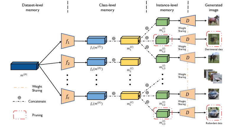
Figure 1: Illustration of Hierarchical Memory Network and pruning. HMN consists of three tiers of memories (which are learnable parameters). $f_{i}$ is the feature extractor for each class. $D$ is a uniform decoder to translate concatenated memories to images. When we identify redundant or detrimental images, the corresponding instance-level memories are pruned, as indicated by red boxes.

Images naturally share features in a hierarchical way due to the inherent hierarchical structure of the classification system. For instance, two images of cats can share common features specific to the cat class, but an image of a cat and another of a dog may still have shared features of the broader animal class. To better align with the hierarchical nature of feature sharing in datasets, we propose a novel data parameterization approach, Hierarchical Memory Network (HMN). Our key insight for HMN is that images from the same class can share class-level common features, and images from different classes can share dataset-level common features. As shown in Figure 1, HMN is a three-tier hierarchical data container to store condensed information. Each tier comprises one or more memory tensors, and memory tensors are learnable parameters. The first tier is a dataset-level memory, $m^{(D)}$, which stores the dataset-level information shared among all images in the dataset. The second tier, the class-level memory, $m^{(C)}_{c}$, where $c$ is the class index. The class-level memories store class-level shared features. The number of class-level memories is equivalent to the number of classes in the dataset. The third tier stores the instance-level memory, $m^{(I)}_{c,i}$, where $c,i$ are the class index and instance index, respectively. The instance-level memories are designed to store unique information for each image. The number of instance-level memories determines the number of images the HMN generates for training. Besides the memory tensors, we also have feature extractors $f_{i}$ for each class and a uniform decoder $D$ to convert concatenated memory to images. Note that both memory tensors and networks count for storage budget calculation.

Other design attempts. In the preliminary stages of designing HMNs, we also considered applying feature extractors between $m^{(C)}_{c}$ and $m^{(I)}_{c,i}$, and attempted to use different decoders for each class to generate images. However, introducing such additional networks did not empirically improve performance. In some cases, it even causes performance drops. One explanation for these performance drops with an increased number of networks is overfitting: more parameters make a condensed dataset better fit the training data and specific model initialization but compromise the model’s generalizability. Consequently, we decided to only apply feature extractors on the dataset-level memory and use a uniform decoder to generate images.

To generate an image for class $c$, we first adopt features extractor $f_{c}$ to extract features from the dataset-level memory . This extraction is followed by a concatenation of these features with the class-level memory $m^{(C)}_{c}$ and instance-level memory $m^{(I)}_{c,i}$. The concatenated memory is then fed to a decoder $D$, which generates the image used for training. Formally, the $i$th generated image, $x_{c,i}$, in the class $c$ is generated by the following formula:

$$x_{c,i}=D([f_{c}(m^{(D)});m^{(C)}_{c};m^{(I)}_{c,i}])$$ (1)

We treat the size of memory tensors and the number of instance-level memories as hyperparameters for architecture design, and we present the detailed configuration for memory tensors, feature extractors, and the decoder for our evaluation in Appendix C. It is also important to note that, in contrast to classic generative models, HMN does not have any input, and the output of HMN is always fixed.

Training loss. HMN can be integrated with various training losses for data condensation. As discussed in Section 2, trajectory-based loss typically exhibits better empirical performance compared to batch-based loss, but it consumes more GPU memory, which may result in scalability issues. In this paper, to ensure better efficiency and scalability for data condensation, we employ gradient matching Kim et al. (2022), a batch-based loss, to condense information into HMNs. Given the original dataset $\mathcal{T}$, the initial model parameter distribution $P_{\theta_{0}}$, the distance function $D$, and loss function $\mathcal{L}$, gradient matching aims to synthesize a dataset $\mathcal{S}$ by solving the following optimization:

$$\min_{\mathcal{S}}\mathbf{E}_{\theta_{0}\sim P_{\theta_{0}}}[\sum_{t=0}^{T-1}D(\nabla_{\theta}\mathcal{L}(\theta_{t},\mathcal{S}),\nabla_{\theta}\mathcal{L}(\theta_{t},\mathcal{T}))],$$ (2)

where $\theta_{t}$ is learned from $\mathcal{T}$ based on $\theta_{t-1}$, and $t$ is the iteration number. In our scenario, the condensed dataset $\mathcal{S}$ is generated by an HMN denoted as $H$. In Section 4.2, our evaluation results show that our data condensation approach, even when employing a batch-based loss, achieves better performance than other DC baselines, including those that utilize high-memory trajectory-based losses.

3.2 Data redundancy in condensed datasets and post-condensation pruning

In this part, we first show that data redundancy exists in condensed datasets in Section 3.2.1. Then, we propose a pruning algorithm on HMN to reduce such data redundancy in Section 3.2.2.

3.2.1 Data redundancy in condensed datasets

Real-world datasets are shown to contain many redundant data Zheng et al. (2023); Pleiss et al. (2020); Toneva et al. (2018). Here, we show that such data redundancy also exists in condensed datasets. We use HaBa Liu et al. (2022) as an example. We first measure the difficulty of training images generated by HaBa with the area under the margin (AUM) Pleiss et al. (2020), a metric measuring data difficulty/importance. The margin for example $(\mathbf{x},y)$ at training epoch $t$ is defined as:

$$M^{(t)}(\mathbf{x},y)=z_{y}^{(t)}(\mathbf{x})-\max_{i\neq y}z_{i}^{(t)}(\mathbf{x}),\vspace{-0.1cm}$$ (3)

where $z_{i}^{(t)}(\mathbf{x})$ is the prediction likelihood for class $i$ at training epoch $t$. AUM is the accumulated margin across all training epochs:

$$\mathbf{AUM}(\mathbf{x},y)=\frac{1}{T}\sum_{t=1}^{T}M^{(t)}(\mathbf{x},y).\vspace{-0.1cm}$$ (4)

Table 1: Coreset selection on the training dataset generated by HaBa on CIFAR10 10IPC. The data with high AUM is pruned first.

Pruning Rate	0	10%	20%	30%	40%
Accuracy (%)	69.5	69.5	68.9	67.6	65.6

A low AUM value indicates that examples are hard to learn. Those examples with lower AUM value are harder to learn, thus are thought to provide more information for training and are more importantToneva et al. (2018); Pleiss et al. (2020); Zheng et al. (2023). Then, as suggested in SOTA coreset selection work Toneva et al. (2018), we prune out the data with smaller importance (high AUM). The results of coreset selection on the dataset generated by HaBa for CIFAR10 10IPC are presented in Table 1. We find that pruning up to 10% of the training examples does not hurt accuracy. This suggests that these 10% examples are redundant and can be pruned to save the storage budget.

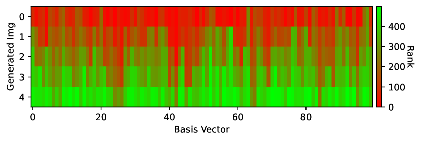
Figure 2: Rank distribution for different basis vectors in HaBa for CIFAR10 10IPC. Each column in this figure represents the difficulty rank of images generated using the same basis vector. The color stands for the difficulty rank among all generated images. Green denotes easy-to-learn (less important) images, while red indicates hard-to-learn (more important) images.

Pruning on generated datasets is straightforward, but pruning relevant weights in data containers can be challenging. SOTA well-performed data parameterization methods, like LinBa and HaBa, use factorization-based methods to generate images. Factorization-based methods use different combinations between basis vectors and decoders to share information, but this also creates interdependence among images, making prune specific images in data containers challenging.

A potential solution for pruning factorization-based data containers is to prune basis vectors in the data containers (each basis vector is used to generate multiple training images). However, we show that directly pruning these basis vectors can lead to removing important data. In Figure 2, we plot the importance rank distribution for training data generated by each basis vector. We observe that the difficulty/importance of images generated by the same basis vector can differ greatly. Thus, simply pruning a basis vector does not guarantee selective pruning of only the desired images.

Different from the factorization-based data condensation algorithm, HMN ensures good independence of each generated instance. As we can see in Figure 1, although generated images share information by using the same dataset-level and class-level memory, each generated image has its own instance-level memory, which allows us to prune redundant generated images by pruning corresponding instance-level memories (as illustrated by red dashed boxes in Figure 1).

3.2.2 Over-budget condensation and post-condensation pruning

To condense datasets with specific storage budgets and take advantage of the pruning property of HMN to further enhance data condensation, we propose to first condense data into over-budget HMNs, which exceed the storage budget by $p\%$ (which is a hyperparameter). Subsequently, we prune these HMNs to fit the allocated storage budget.

Inspired by recent coreset research Zheng et al. (2023) showing that pruning both easy and hard data leads to better coreset, we present a double-end pruning algorithm with an adaptive hard pruning rate to prune data adaptively for different storage budgets. As shown in Algorithm 1, given an over-budget HMN containing $k$ more generated images per class than allowed by the storage budget, we employ grid search to determine an appropriate hard pruning rate, denoted as $\beta$ (Line 4 to Line 12). We then prune $\lfloor\beta k\rfloor$ of the lowest AUM (hardest) examples and $k-\lfloor\beta k\rfloor$ of the highest AUM (easiest) examples by removing the corresponding instance-level memory for each class. The pruning is always class-balanced: the pruned HMNs generate the same number of examples for each class.

Algorithm 1 Over-budget HMN Double-end Pruning

1:  Input: Over-budget HMN: $H$; Over-budget images per class: $k$; $\beta$ search space $\mathcal{B}$.

2:  Condensed dataset $\mathcal{S}\leftarrow H()$; $Acc_{best}=0$; $\mathcal{S}_{best}=\emptyset$;

3:  Calculate AUM for all examples in $\mathcal{S}$ based on Equation 4;

4:  for $\beta$ in $\mathcal{B}$ do

5:     $\widetilde{\mathcal{S}}\leftarrow\mathcal{S}.clone()$;

6:     Prune $\lfloor\beta k\rfloor$ of the lowest AUM examples for each class from $\widetilde{\mathcal{S}}$;

7:     Prune $k-\lfloor\beta k\rfloor$ of the highest AUM examples for each class from $\widetilde{\mathcal{S}}$;

8:     $Acc\leftarrow$ Test accuracy of the model trained on $\widetilde{\mathcal{S}}$;

9:     if $Acc>Acc_{best}$ then

10:        $Acc_{best}=Acc$; $\widetilde{\mathcal{S}}_{best}=\widetilde{\mathcal{S}}$;

11:     end if

12:  end for

13:  $\Delta\mathcal{S}=\mathcal{S}-\widetilde{\mathcal{S}}_{best}$;

14:  $\widetilde{H}\leftarrow$ Prune corresponding instance-level memories in $H$ based on $\Delta\mathcal{S}$;

15:  Output: Pruned in-budget network: $\widetilde{H}$.

Additional pruning may introduce additional computational costs compared to the standard data condensation pipeline. However, we contend that, compared to the time required for data condensation, the pruning step requires a relatively small computation time. For example, while data condensation with HMNs for CIFAR10 1IPC needs about 15 hours on a 2080TI GPU, the coreset selection on the condensed dataset only costs an additional 20 minutes.

4 Experiments

In this section, we compare the performance of HMN to SOTA baselines in Section 4.2 and discuss the impacts of post-condensation pruning and HMN architecture design in Section 4.3. We also evaluate HMN on continual learning tasks in Section 4.4. Due to the page limitation, we include additional evaluation results in Appendix D: We compare the transferability of datasets generated by HMNs and other baselines in Appendix D.1. We then study the relationship between pruning rate and accuracy in Appendix D.3. Subsequently, we do data profiling and study the data redundancy on the condensed datasets synthesized by different DC methods in Appendix D.4. Lastly, we visualize the condensed training data generated by HMNs for different datasets in Appendix D.5.

4.1 Experimental Settings

Datasets and training settings We evaluate our proposed method on four public datasets: CIFAR10, CIFAR100 (Krizhevsky et al., 2009), SVHN (Netzer et al., 2011), and Tiny-ImageNet (Deng et al., 2009) under three different storage budgets: 1/10/50IPC (For Tiny-ImageNet, due to the computation limitation, we conduct the evaluation on 1/10IPC). Following previous works Zhao & Bilen (2021); Liu et al. (2022); Deng & Russakovsky (2022), we select ConvNet, which contains three convolutional layers followed by a pooling layer, as the network architecture for data condensation and classifier training. For the over-budget training and post-condensation, we first conduct a pruning study on HMNs in Section D.3, we observed that there is a pronounced decline in accuracy when the pruning rate exceeds 10%. Consequently, we select 10% as the over-budget rate for all settings. Nevertheless, we believe that this rate choice could be further explored, and other rate values could potentially further enhance the performance of HMNs. Due to space limits, we include more HMN architecture details, experimental settings, and additional implementation details in the supplementary material. All data condensation evaluation is repeated $3$ times, and training on each HMN is repeated $10$ times with different random seeds to calculate the mean with standard deviation.

Table 2: The performance (test accuracy %) comparison to state-of-the-art methods. The baseline method’s accuracy is obtained from data presented in original papers or author-implemented repos. We label the methods using the trajectory-based training loss consuming larger GPU memory with a star (*). We highlight the highest accuracy among all methods and methods with batch-based loss.

Container

Dataset

CIFAR10

CIFAR100

SVHN

Tiny

IPC

1

10

50

1

10

50

1

10

50

1

10

Image

DC

$28.3$ $\scriptscriptstyle\pm 0.5$

$44.9$ $\scriptscriptstyle\pm 0.5$

$53.9$ $\scriptscriptstyle\pm 0.5$

$12.8$ $\scriptscriptstyle\pm 0.3$

$25.2$ $\scriptscriptstyle\pm 0.3$

-

$31.2$ $\scriptscriptstyle\pm 1.4$

$76.1$ $\scriptscriptstyle\pm 0.6$

$82.3$ $\scriptscriptstyle\pm 0.3$

$4.6$ $\scriptscriptstyle\pm 0.6$

$11.2$ $\scriptscriptstyle\pm 1.6$

DSA

$28.8$ $\scriptscriptstyle\pm 0.7$

$52.1$ $\scriptscriptstyle\pm 0.5$

$60.6$ $\scriptscriptstyle\pm 0.5$

$13.9$ $\scriptscriptstyle\pm 0.3$

$32.3$ $\scriptscriptstyle\pm 0.3$

$42.8$ $\scriptscriptstyle\pm 0.4$

$27.5$ $\scriptscriptstyle\pm 1.4$

$79.2$ $\scriptscriptstyle\pm 0.5$

$84.4$ $\scriptscriptstyle\pm 0.4$

$6.6$ $\scriptscriptstyle\pm 0.2$

$14.4$ $\scriptscriptstyle\pm 2.0$

DM

$26.0$ $\scriptscriptstyle\pm 0.8$

$48.9$ $\scriptscriptstyle\pm 0.6$

$63.0$ $\scriptscriptstyle\pm 0.4$

$11.4$ $\scriptscriptstyle\pm 0.3$

$29.7$ $\scriptscriptstyle\pm 0.3$

$43.6$ $\scriptscriptstyle\pm 0.4$

-

-

-

$3.9$ $\scriptscriptstyle\pm 0.2$

$12.9$ $\scriptscriptstyle\pm 0.4$

CAFE+DSA

$31.6$ $\scriptscriptstyle\pm 0.8$

$50.9$ $\scriptscriptstyle\pm 0.5$

$62.3$ $\scriptscriptstyle\pm 0.4$

$14.0$ $\scriptscriptstyle\pm 0.3$

$31.5$ $\scriptscriptstyle\pm 0.2$

$42.9$ $\scriptscriptstyle\pm 0.2$

$42.9$ $\scriptscriptstyle\pm 3.0$

$77.9$ $\scriptscriptstyle\pm 0.6$

$82.3$ $\scriptscriptstyle\pm 0.4$

-

-

MTT*

$46.3$ $\scriptscriptstyle\pm 0.8$

$65.3$ $\scriptscriptstyle\pm 0.7$

$71.6$ $\scriptscriptstyle\pm 0.2$

$24.3$ $\scriptscriptstyle\pm 0.3$

$40.1$ $\scriptscriptstyle\pm 0.4$

$47.7$ $\scriptscriptstyle\pm 0.2$

$58.5$ $\scriptscriptstyle\pm 1.4$

$70.8$ $\scriptscriptstyle\pm 1.8$

$85.7$ $\scriptscriptstyle\pm 0.1$

$8.8$ $\scriptscriptstyle\pm 0.3$

$23.2$ $\scriptscriptstyle\pm 0.2$

Data Parame- -terization

IDC

$50.0$ $\scriptscriptstyle\pm 0.4$

$67.5$ $\scriptscriptstyle\pm 0.5$

$71.6$ $\scriptscriptstyle\pm 0.2$

-

$44.8$

-

$68.5$

$87.5$

$90.1$

-

-

HaBa*

$48.3$ $\scriptscriptstyle\pm 0.8$

$69.9$ $\scriptscriptstyle\pm 0.4$

$74.0$ $\scriptscriptstyle\pm 0.2$

$33.4$ $\scriptscriptstyle\pm 0.4$

$40.2$ $\scriptscriptstyle\pm 0.2$

$47.0$ $\scriptscriptstyle\pm 0.2$

$69.8$ $\scriptscriptstyle\pm 1.3$

$83.2$ $\scriptscriptstyle\pm 0.4$

$88.3$ $\scriptscriptstyle\pm 0.1$

-

-

LinBa*

$\mathbf{66.4}$ $\scriptscriptstyle\mathbf{\pm 0.4}$

$71.2$ $\scriptscriptstyle\pm 0.4$

$73.6$ $\scriptscriptstyle\pm 0.5$

$34.0$ $\scriptscriptstyle\pm 0.4$

$42.9$ $\scriptscriptstyle\pm 0.7$

-

$87.3$ $\scriptscriptstyle\pm 0.1$

$89.1$ $\scriptscriptstyle\pm 0.2$

$89.5$ $\scriptscriptstyle\pm 0.2$

$16.0$ $\scriptscriptstyle\pm 0.7$

-

HMN (Ours)

$\mathbf{65.7}$ $\scriptscriptstyle\mathbf{\pm 0.3}$

$\mathbf{73.7}$ $\scriptscriptstyle\mathbf{\pm 0.2}$

$\mathbf{76.9}$ $\scriptscriptstyle\mathbf{\pm 0.2}$

$\mathbf{36.3}$ $\scriptscriptstyle\mathbf{\pm 0.2}$

$\mathbf{45.4}$ $\scriptscriptstyle\mathbf{\pm 0.2}$

$\mathbf{48.5}$ $\scriptscriptstyle\mathbf{\pm 0.2}$

$\mathbf{87.4}$ $\scriptscriptstyle\mathbf{\pm 0.2}$

$\mathbf{90.0}$ $\scriptscriptstyle\mathbf{\pm 0.1}$

$\mathbf{91.2}$ $\scriptscriptstyle\mathbf{\pm 0.1}$

$\mathbf{19.4}$ $\scriptscriptstyle\mathbf{\pm 0.1}$

$\mathbf{24.4}$ $\scriptscriptstyle\mathbf{\pm 0.1}$

Entire Dataset

$84.8_{\pm 0.1}$

$56.2_{\pm 0.3}$

$95.4_{\pm 0.1}$

$37.6_{\pm 0.4}$

Baselines. We compare our proposed method with eight baselines, which can be divided into two categories by data containers: 1) Image data container. We use five recent works as the baseline: MTT Cazenavette et al. (2022) (as mentioned in Section 2). DC Zhao et al. (2021) and DSA Zhao & Bilen (2021) optimize condensed datasets by minimizing the distance between gradients calculated from a batch of condensed data and a batch of real data. DM Zhao & Bilen (2023b) aims to encourage condensed data to have a similar distribution to the original dataset in latent space. Finally, CAFE Wang et al. (2022) improves the distribution matching idea by layer-wise feature alignment. 2) Data parameterization. We also compare our method with three SOTA data parameterization baselines. IDC Kim et al. (2022) enhances gradient matching loss calculation strategy and employs multi-formation functions to parameterize condensed data. HaBa Liu et al. (2022) and LinBa Deng & Russakovsky (2022) concurrently proposes factorization-based data parameterization to achieve information sharing among different generated images.

Besides grouping the methods by data containers, we also categorize those methods by the training losses used. As discussed in Section 2, there are two types of training loss: trajectory-based training loss and batch-based training loss. In Table 2, we highlight the methods using a trajectory-based loss with a star (*). In our HMN implementation, we condense our HMNs with gradient matching loss used in Kim et al. (2022), which is a low GPU memory consumption batch-based loss.

The storage budget calculation. As with other data parameterization techniques, our condensed data does not store images but rather model parameters. To ensure a fair comparison, we adopt the same setting of previous works Liu et al. (2022); Deng & Russakovsky (2022) and consider the total number of model parameters (including both memory tensors and networks) as the storage budget (assuming that numbers are stored as floating-point values). For instance, the storage budget for CIFAR10 1IPC is calculated as $32*32*3*1*10=30,720$. The HMN for CIFAR10 1IPC always has an equal or lower number of parameters than this number.

4.2 Data Condensation Performance Comparison

We compare HMN with eight baselines on four different datasets (CIFA10, CIFAR100, SVHN, and Tiny ImageNet) in Table 2. We divide all methods into two categories by the type of data container formats: Image data container and data parameterization container. We also categorize all methods by the training loss. We use a star (*) to highlight the methods using a trajectory-based loss. The results presented in Table 2 show that HMN achieves comparable or better performance than all baselines. It is worth noting that HMN is trained with gradient matching, which is a low GPU memory loss. Two other well-performed data parameterization methods, HaBa and LinBa, are all trained with trajectory-based losses, consuming much larger GPU memory. As far as we know, HMN is the first method to achieve such good performance with a low GPU memory loss. These results show that batch-based loss can still achieve very good performance with an effective data parameterization method and help address the memory issue of data condensation Cazenavette et al. (2022); Cui et al. (2022); Cazenavette et al. (2023). We believe that HMN provides a strong baseline for exploring data condensation with limited GPU memory. We further study the memory consumed by different data parameterization methods in Appendix D.2

Table 3: Accuracy (%) performance comparison to data containers with the same gradient matching training loss on CIFAR10. The evaluation results show that HMN outperforms all other data parameterization methods substantially.

Data Container	1IPC	10IPC	50IPC
Image	36.7	58.3	69.5
IDC	50.0	67.5	74.5
HaBa	48.5	61.8	72.4
LinBa	62.0	67.8	70.7
HMN (Ours)	65.7	73.7	76.9

Data parameterization comparison with the same loss. In addition to the end-to-end method comparison presented in Table 2, we also compare HMN with other data parameterization methods with the same training loss (gradient matching loss used by IDC) for a fairer comparison. The results are presented in Table 3. After replacing the trajectory-based loss used by HaBa and LinBa with a batch-based loss, there is a noticeable decline in accuracy (but HaBa and LinBa still outperform the image data container). HMN outperforms other data parameterization by a larger margin when training with the same training loss, which indicates that HMN is a more effective data parameterization method and can condense more information within the same storage budget.

4.3 Ablation Studies

Table 4: Performance comparison on different pruning strategies on HMN. Double-end is the pruning strategy introduced in Algorithm 1. In-budget stands for HMNs are condensed within the allocated storage budget.

IPC	1	10	50
Double-end	$\mathbf{65.7}$	$\mathbf{73.7}$	$\mathbf{76.9}$
Prune easy	$65.3$	$73.1$	$76.6$
Random	$65.2$	$72.9$	$75.3$
In-budget	$65.1$	$73.2$	$75.4$

Ablation study on pruning. In Table 4, we explore the performance of different pruning strategies applied to over-budget HMNs on the CIFAR10 dataset. The strategy termed "Prune easy" is widely employed in conventional coreset selection methods Coleman et al. (2019); Toneva et al. (2018); Paul et al. (2021); Xia et al. (2023), which typically prioritize pruning of easy examples containing more redundant information. “In-budget" refers to the process of directly condensing HMNs to fit the storage budgets, which does not need any further pruning. As shown in Table 4, our proposed pruning strategy (double-end) outperforms all other pruning strategies. We also observe that, as the storage budget increases, the accuracy improvement becomes larger compared to “in-budget” HMNs. We think this improvement is because a larger storage budget causes more redundancy in the condensed data Cui et al. (2022), which makes pruning reduce more redundancy in condensed datasets. Also, the performance gap between the “Prune easy" strategy and our pruning method is observed to narrow as the storage budget increases. This may be attributed to larger storage budgets for HMNs leading to more redundant easy examples. The “Prune easy" strategy can be a good alternative for pruning for large storage budgets.

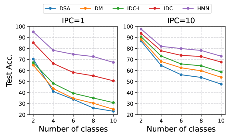
Figure 3: Continual learning evaluation on CIFAR10. In the class incremental setting with 2 incoming classes per stage, HMN outperforms existing methods (including DSA, DM and IDC) under different storage budgets.

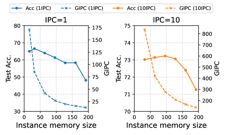
Figure 4: Instance-memory length vs. Accuracy for CIFAR10 HMNs with 1IPC/10IPC storage budgets. GIPC refers to the number of generated images per class. The solid and dashed curves represent the accuracy and GIPC, respectively.

Instance-memory size v.s. Retrained model accuracy. In an HMN, every generated image is associated with an independent instance-level memory, which constitutes the majority of the storage budget. Consequently, given a fixed storage budget, an increase in the instance-level memory results in a decrease in the number of generated images per class (GIPC). In Figure 4, we explore the interplay between the instance-memory size, the accuracy of the retrained model, and GIPC. Specifically, we modify the instance-level memory size of CIFAR10 HMNs for given storage budgets of 1IPC and 10IPC. (It should be noted that for this ablation study, we are condensing in-budget HMNs directly without employing any coreset selection on the condensed HMNs.)

From Figure 4, we observe that an increase in the instance-level memory size leads to a swift drop in GIPC, as each generated image consumes a larger portion of the storage budget. Moreover, we notice that both excessively small and large instance-level memory sizes negatively affect the accuracy of retrained models. Reduced instance-level memory size can result in each generated image encoding only a limited amount of information. This constraint can potentially deteriorate the quality of the generated images and negatively impact training performance. Conversely, while an enlarged instance-level memory size enhances the volume of information encoded in each image, it precipitously reduces GIPC. This reduction can compromise the diversity of generated images for training. For instance, with a 1IPC storage budget, an increase in the instance-level memory size, leading to a decrease in GIPC from $85$ to $13$, results in an accuracy drop from $65.1\%$ to $48.2\%$.

4.4 Continual Learning Performance Comparison

Following the same setting in DM Zhao & Bilen (2023a) and IDC Kim et al. (2022), we evaluate the effectiveness of HMN in an application scenario of continual learning Bang et al. (2021); Rebuffi et al. (2017b); Chaudhry et al. (2019). Specifically, we split the whole training phase into 5 stages, i.e. 2 classes per stage. At each stage, we condense the data currently available at this stage with ConvNet. As illustrated in Figure 4, evaluated on ConvNet models under the storage budget of both 1 IPC and 10 IPC, HMN obtains better performance compared with DSA Zhao & Bilen (2021), DM Zhao & Bilen (2023b), and IDC Kim et al. (2022). Particularly, in the low storage budget scenario, i.e. 1 IPC, the performance improvement brought by HMN is more significant, up to 16%. The results indicate that HMNs provide higher-quality condensed data and boost continual learning performance.

5 Acknowledgements

This work was partially supported by DARPA under agreement number 885000. This work was performed under the auspices of the U.S. Department of Energy by the Lawrence Livermore National Laboratory under Contract No. DE- AC52-07NA27344 and was supported by the LLNL-LDRD Program under Project No. 22-SI-004.

6 Conclusion

This paper introduces a novel data parameterization architecture, Hierarchical Memory Network (HMN), which is inspired by the hierarchical nature of common feature sharing in datasets. In contrast to previous data parameterization methods, HMN aligns more closely with this hierarchical nature of datasets. Additionally, we also show that redundant data exists in condensed datasets. Unlike previous data parameterization methods, although HMNs achieve information sharing among generated images, HMNs also naturally ensure good independence between images, which facilitates the pruning of the data containers. The evaluation results on four public datasets shows that HMN outperforms DC baselines, indicating that HMN is a more efficient architecture for data condensation.

Appendix A Appendix Overview

In this appendix, we provide more details on our experimental setting and additional evaluation results. In Section B, we discuss the computation cost caused by data parameterization. In Section C, we introduce the detailed setup of our experiment to improve the reproducibility of our paper. In Section D, we conduct additional studies on how the pruning rate influences the model performance. In addition, we visualize images generated by HMNs in Section D.5.

Appendix B Discussion

While data parameterization methods demonstrate effective performance in data condensation, we show that generated images per class (GIPC) play an important role in data parameterization (as we discussed in Section 4.3). The payoff is that HMNs, along with other SOTA data parameterization methods Kim et al. (2022); Deng & Russakovsky (2022); Liu et al. (2022) invariably generate a higher quantity of images than those condensed and stored in pixel space with a specific storage budget, which may potentially escalate the cost of data condensation. A limitation of HMNs and other data parameterization methods is that determining the parameters of the data container to achieve high-quality data condensation can be computationally demanding. A key challenge and promising future direction are to explore approaches to reduce GIPC without affecting the data condensation performance.

Appendix C Experiment Setting and Implementation Details

C.1 HMN architecture design.

In this section, we introduce more details on the designs of the Hierarchical Memory Network (HMN) architecture, specifically tailored for various datasets and storage budgets. We first introduce the three-tier hierarchical memories incorporated within the network. Subsequently, we present the neural network designed to convert memory and decode memories into images utilized for training.

Table 5: The detailed three-tier memory settings. We use the same setting for CIFAR10 and SVHN. #Instance-level memory is the number of memory fitting the storage budget. #Instance-level memory (Over-budget) indicates the actual number of instance-level memory that we use for condensation, and we prune this number to #Instance-level memory after condensation.

Dataset	SVHN & CIFAR10			CIFAR100			Tiny
IPC	1	10	50	1	10	50	1	10
Dataset-level memory channels	5	50	50	5	50	50	30	50
Class-level memory channels	3	30	30	3	30	30	20	30
Instance-level memory channels	2	6	8	2	8	14	4	10
#Instance-level memory	85	278	1168	93	219	673	42	185
#Instance-level memory (Over-budget)	93	306	1284	102	243	740	46	203

Hierarchical memories. HMNs consist of three-tier memories: dataset-level memory $m^{(D)}$, class-level memory $m^{(C)}_{c}$, and instance-level memory $m^{(I)}_{c,i}$, which are supposed to store different levels of features of datasets. Memories of HMNs for SVHN, CIFAR10, and CIFAR100 have a shape of (4, 4, Channels), and memories for Tiny ImageNet have a shape of (8, 8, Channels), where the number of channels is a hyper-parameter for different settings. We present the detailed setting for the number of channels and the number of memories under different data condensation scenarios in Table 5. Besides the channels of memories, we also present the number of instance-level of memories. Every HMN has only one dataset-level memory, and the number of class-level memory is equal to the number of classes in the dataset. The number of instance-level memory for the over-budget class leads to an extra 10% storage budget cost, which will be pruned by post-condensation pruning.

Decoders. In addition to three-tier memories, each HMN has two types of networks: 1) A dataset-level memory feature extractor for each class; 2) A uniform decoder to convert memories to images for model training. Dataset-level memory feature extractors $f_{c}$ are used to extract features from the dataset-level memory for each class. For 1IPC storage budget setting, we use the identity function as the feature extractor to save the storage budget. For 10IPC and 50IPC storage budget settings, the feature extractors consist of a single deconvolutional layer with the kernel with 1 kernel size and $40$ output channels. The uniform decoder $D$ is used to generate images for training. In this paper, we adopt a classic design of decoder for image generation, which consist of a series of deconvolutional layers and batch normalization layers: ConvTranspose(Channels of memory, 10, 4, 1, 2) $\to$ Batch Normalization $\to$ ConvTranspose(10, 6, 4, 1, 2) $\to$ Batch Normalization $\to$ ConvTranspose(6, 3, 4, 1, 2). The arguments for ConvTranspose is input-channels, output-channels, kernel size, padding, and stride, respectively. The “Channels of memory” is equal to the addition of the channels of the output of $f_{c}$, the class-level memory channels, and the instance-level memory channels. When we design the HMN architecture, we also tried the design with different decoders for different classes. However, we find that it experiences an overfitting issue and leads to worse empirical performance.

C.2 Training settings.

Data condensation. Following previous works Zhao & Bilen (2021); Liu et al. (2022); Deng & Russakovsky (2022), we select ConvNet, which contains three convolutional layers followed by a pooling layer, as the network architecture for data condensation and classifier training for all three datasets. We employ gradient matching Kim et al. (2022); Liu et al. (2022), a batch-based loss with low GPU memory consumption, to condense information into HMNs. More specifically, our code is implemented based on IDC Liu et al. (2022). For all datasets, we set the number of inner iterations to 200 for gradient matching loss. The total number of training epochs for data condensation is 1000. We use the Adam optimizer ($\beta_{1}=0.9$ and $\beta_{2}=0.99$) with a 0.01 initial learning rate (0.02 initial learning rate for CIFAR100) for data condensation. The learning rate scheduler is the step learning rate scheduler, and the learning rate will time a factor of $0.1$ at $600$ and $800$ epochs. We use the mean squared error loss for calculating the distance of gradients for CIFAR10 and SVHN, and use L1 loss for the CIFAR100 and Tiny ImageNet. To find the best hard pruning rate $\beta$ in Algorithm 1, we perform a grid search from 0 to 0.9 with a 0.1 step. All experiments are run on a combination of RTX2080TI, RTX3090, A40, and A100, depending on memory usage and availability.

Model training with HMNs. For CIFAR10, we train the model with datasets generated by HMNs for 2000, 2000, and 1000 epochs for 1IPC, 10IPC, and 50IPC, respectively. We use the SGD optimizer (0.9 momentum and 0.0002 weight decay) with a 0.01 initial learning rate. The learning rate scheduler is the cosine annealing learning rate scheduler Loshchilov & Hutter (2017) with a $0.0001$ minimum learning rate. For CIFAR100, we train the model with datasets generated by HMNs for 500 epochs. We use the SGD optimizer ($0.9$ momentum and $0.0002$ weight decay) with a $0.01$ initial learning rate. The learning rate scheduler is the cosine annealing learning rate scheduler Loshchilov & Hutter (2017) with a $0.0001$ minimum learning rate. For SVHN, we train the model with datasets generated by HMNs for 1500, 1500, 700 epochs for 1IPC, 10IPC, and 50IPC, respectively. We use the SGD optimizer (0.9 momentum and 0.0002 weight decay) with a 0.01 initial learning rate. For SVHN, we train the model with datasets generated by HMNs for 300 epochs for both 1IPC and 10IPC settings. We use the SGD optimizer (0.9 momentum and 0.0002 weight decay) with a 0.02 initial learning rate. The learning rate scheduler is the cosine annealing learning rate scheduler Loshchilov & Hutter (2017) with a $0.0001$ minimum learning rate. Similar to Liu et al. (2022), we use the DSA augmentation Zhao & Bilen (2021) and CutMix as data augmentation for data condensation and model training on HMNs.

Continual learning. Following the class incremental setting of Kim et al. (2022), we adopt distillation loss Li & Hoiem (2018) and train the model constantly by loading weights of the previous stage and expanding the output dimension of the last fully-connected layer Rebuffi et al. (2017a). Specifically, we use a ConvNet-3 model trained for 1000 epochs at each stage, using SGD with a momentum of 0.9 and a weight decay of $5e-4$. The learning rate is set to 0.01, and decays at epoch 600 and 800, with a decaying factor of 0.2.

Appendix D Additional Evaluation Results

In this section, we present additional evaluation results to further demonstrate the efficacy of HMNs. We compare the transferability of datasets generated by HMNs and other baselines in Section D.1. We then study the relationship between pruning rate and accuracy in Section D.3. Subsequently, we do data profiling and study the data redundancy on the condensed datasets synthesized by different DC methods in Section D.4. Lastly, we visualize the condensed training data generated by HMNs for different datasets in Section D.5.

D.1 Cross-architecture Transferability

Table 6: Transferability (accuracy %) comparison to different model architectures. Due to the extremely long training time, we cannot reproduce the results on LinBa. Compared with IDC and HaBa, we find that HMN achieves better performance for all model architectures.

IPC	1			10			50
Method	HMN	IDC	HaBa	HMN	IDC	HaBa	HMN	IDC	HaBa
ConvNet	65.7	49.2	48.3	73.7	64.8	69.9	76.9	73.1	74
VGG16	58.5	28.7	34.1	64.3	43.1	53.8	70.2	57.9	61.1
ResNet18	56.8	32.3	36.0	62.9	45.1	49.0	69.1	58.4	60.4
DenseNet121	50.7	24.3	34.6	56.9	38.5	49.3	65.1	50.5	57.8

To investigate the generalizability of HMNs across different architectures, we utilized condensed HMNs to train other network architectures. Specifically, we condense HMNs with ConvNet, and the condensed HMNs are tested on VGG16, ResNet18, and DenseNet121. We compare our methods with two other data parameterization methods: IDC and HaBa. (Due to the extremely long training time, we are unable to reproduce the results in LinBa). The evaluation results on CIFAR10 are presented in Table 6. We find that HMNs consistently outperform other baselines. Of particular interest, we observe that VGG16 has a better performance than ResNet18 and DenseNet121. A potential explanation may lie in the architectural similarities between ConvNet and VGG16. Both architectures are primarily comprised of convolutional layers and lack skip connections.

D.2 GPU Memory comparison

Table 7: Performance and memory comparison between LinBa, HaBa, and HMN trained with suggested loss in corresponding papers on CIFAR10.

IPC	Method	Loss	Acc.	Memory
1	HaBa	MTT	48.3	3368M
	LinBa	BPTT	66.4	OOM
	HMN (Ours)	GM-IDC	65.7	2680M
10	HaBa	MTT	69.9	11148M
	LinBa	BPTT	71.2	OOM
	HMN (Ours)	GM-IDC	73.7	4540M
50	HaBa	MTT	74	48276M
	LinBa	BPTT	73.6	OOM
	HMN (Ours)	GM-IDC	76.9	10426M

As discussed in Section 4.1, GPU memory consumption can be very different depending on the training losses used. We compare the GPU memory used by HMN with two other well-performed data parameterization methods, HaBa and LinBa. As depicted by Table 7, HMN achieves better or comparable performance compared to HaBa and LinBa with much less GPU memory consumption. Specifically, LinBa is trained with BPTT with a very long trajectory, which leads to extremely large GPU memory consumption. LinBa official implementation offloads the GPU memory to CPU memory to address this issue. However, the context switch in memory offloading causes the training time to be intolerable. For example, LinBa needs about 14 days to condense a CIFAR10 1IPC dataset with a 2080TI, but using HMN with gradient matching only needs 15 hours to complete training on a 2080TI GPU. Although this memory saving does not come from the design of HMN, our paper shows that batch-based loss can still achieve very good performance with a proper data parameterization method, which helps address the memory issue of data condensation Cazenavette et al. (2022); Cui et al. (2022); Cazenavette et al. (2023).

D.3 Pruning Rate v.s. Accuracy

In this section, we examine the correlation between accuracy and pruning rates on HMNs. The evaluation results are presented in Figure 6. We observe that the accuracy drops more as the pruning rates increase, and our double-end pruning algorithm consistently outperforms random pruning. Furthermore, we observe that an increasing pruning rate results in a greater reduction in accuracy for HMNs with smaller storage budgets. For instance, when the pruning rate increases from 0 to 30%, models trained on the 1IPC HMN experience a significant drop in accuracy, plunging from 66.2% to 62.2%. Conversely, models trained on the 50IPC HMN exhibit a mere marginal decrease in accuracy, descending from 76.7% to 76.5% with the same increase in pruning rate. This discrepancy may be attributed to the fact that HMNs with larger storage budgets generate considerably more redundant data. Consequently, pruning such data does not significantly impair the training performance.

D.4 Data Profiling on SOTA Methods

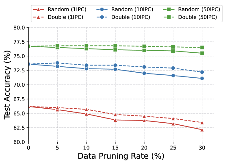
Figure 5: Relationship between pruning rates and accuracy on HMNs for CIFAR10. All HMNs are over-budget HMNs (10% extra). Different colors stand for different storage budgets. Solid lines stand for random pruning and dashed lines stand for double-end pruning.

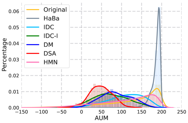
Figure 6: The distribution of AUM of CIFAR10 training images synthesized by different approaches. Different colors denote different data condensation approaches. Data parameterization based methods have more redundant images.

Figure 6 illustrates the distribution of AUM of images synthesized by different data condensation approaches, as well as the original data, denoted as “Original". We calculate the AUM by training a ConvNet for 200 epochs. We observe that approaches (IDC-I Kim et al. (2022), DM Zhao & Bilen (2023a), and DSA Zhao & Bilen (2021)) that condense data into pixel space typically synthesize fewer images with a high AUM value. In contrast, methods that rely on data parameterization, such as HaBa Liu et al. (2022), IDC Kim et al. (2022), and HMN , tend to produce a higher number of high-aum images. Notably, a large portion of images generated by HaBa exhibit an AUM value approaching 200, indicating a significant amount of redundancy that could potentially be pruned for enhanced performance. However, due to its factorization-based design, HaBa precludes the pruning of individual images from its data containers, which limits the potential for efficiency improvements.

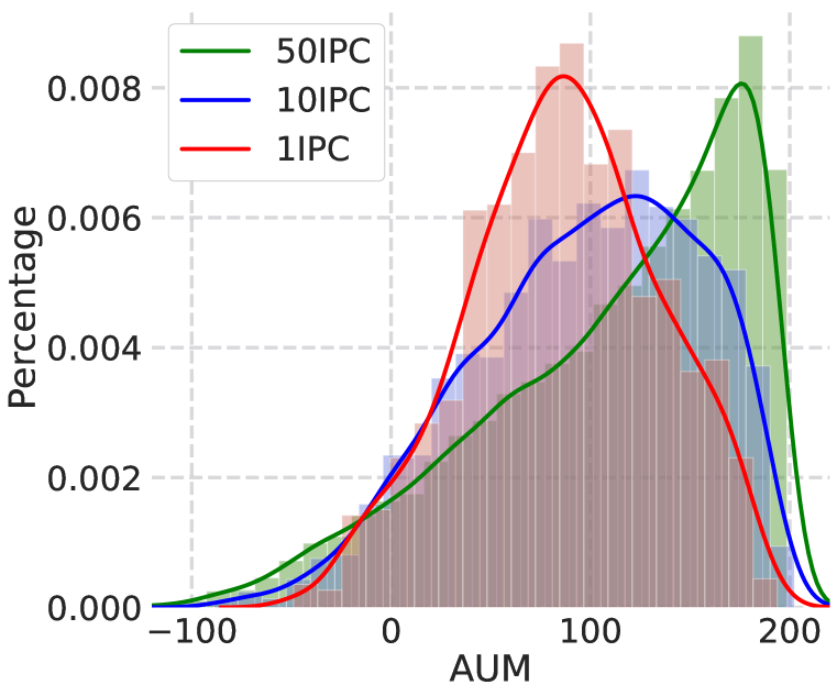
Figure 7: AUM distribution of images generated by HMNs for CIFAR10 with different storage budgets, denoted by different colors.

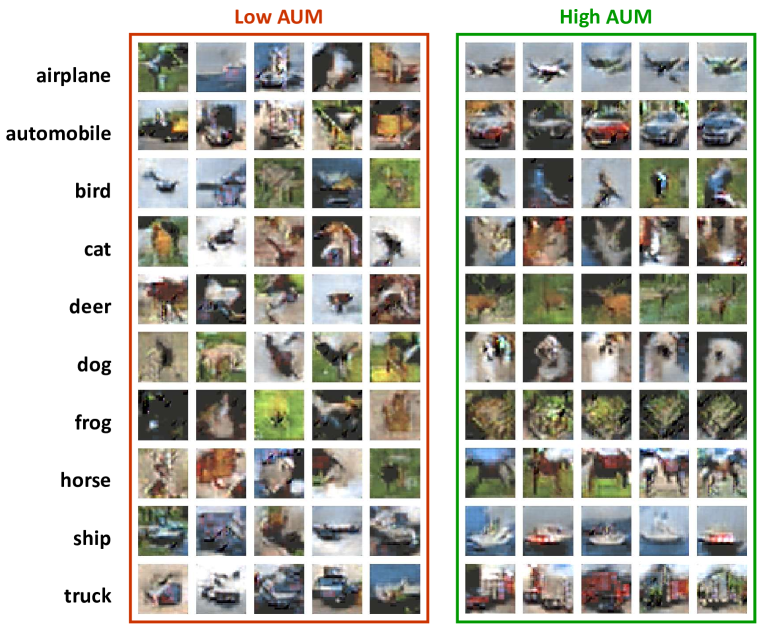
Figure 8: Visualization of the lowest and highest AUM examples generated by a 10IPC HMN of CIFAR10. Each row represents a class.

Moreover, we conduct a more detailed study on the images generated by HMNs. We calculate the AUM by training a ConvNet for $200$ epochs. As shown in Figure 8, many examples possess negative AUM values, indicating that they are likely hard-to-learn, low-quality images that may negatively impact training. Moreover, a considerable number of examples demonstrate AUM values approximating $200$, representing easy-to-learn examples that may contribute little to the training process. We also observe that an increased storage budget results in a higher proportion of easier examples. This could be a potential reason why data condensation performance degrades to random selection when the storage budget keeps increasing, which is observed in Cui et al. (2022): more storage budgets add more easy examples which only provide redundant information and do not contribute much to training. From Figure 8, we can derive two key insights: 1) condensed datasets contain easy examples (AUM close to $200$) as well as hard examples (AUM with negative values), and 2) the proportion of easy examples varies depending on the storage budget.

Additionally, in Figure 8, we offer a visualization of images associated with the highest and lowest AUM values generated by an HMN. It is observable that images with low AUM values exhibit poor alignment with their corresponding labels, which may detrimentally impact the training process. Conversely, images corresponding to high AUM values depict a markedly improved alignment with their classes. However, these images may be overly similar, providing limited information to training.

D.5 Visualization

To provide a better understanding of the images generated by HMNs, we visualize generated images with different AUM values on CIFAR10, CIFAR100, and SVHN with 1.1IPC/11IPC/55IPC storage budgets in this section The visualization results are presented in the following images.

Similar to what we observe in Section 3.2 in the main paper, images with a high AUM value are better aligned with their respective labels. Conversely, images with a low AUM value typically exhibit low image quality or inconsistencies between their content and associated labels. For instance, in the visualizations of SVHNs (depicted in Figures 15 16 17), the numbers in the generated images with a high AUM value are readily identifiable, but content in the generated images with a low AUM value is hard to recognize. Those images are misaligned with their corresponding labels and can be detrimental to training. Pruning on those images can potentially improve training performance. Furthermore, we notice an enhancement in the quality of images generated by HMNs when more storage budgets are allocated. This improvement could be attributable to the fact that images generated by HMNs possess an enlarged instance-level memory, as indicated in Table 5. A larger instance-level memory stores additional information, thereby contributing to better image generation quality.

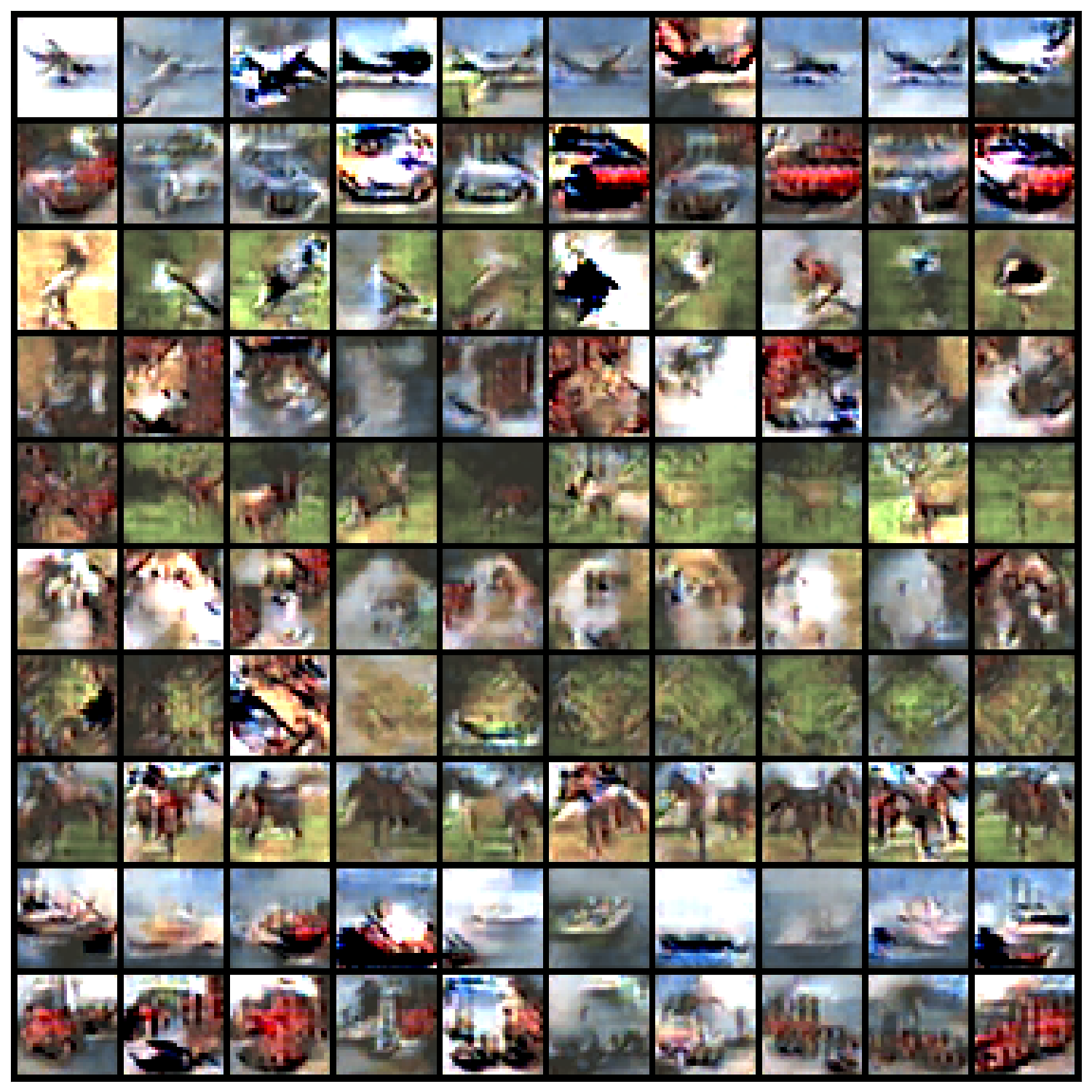
High AUM (Easy) data

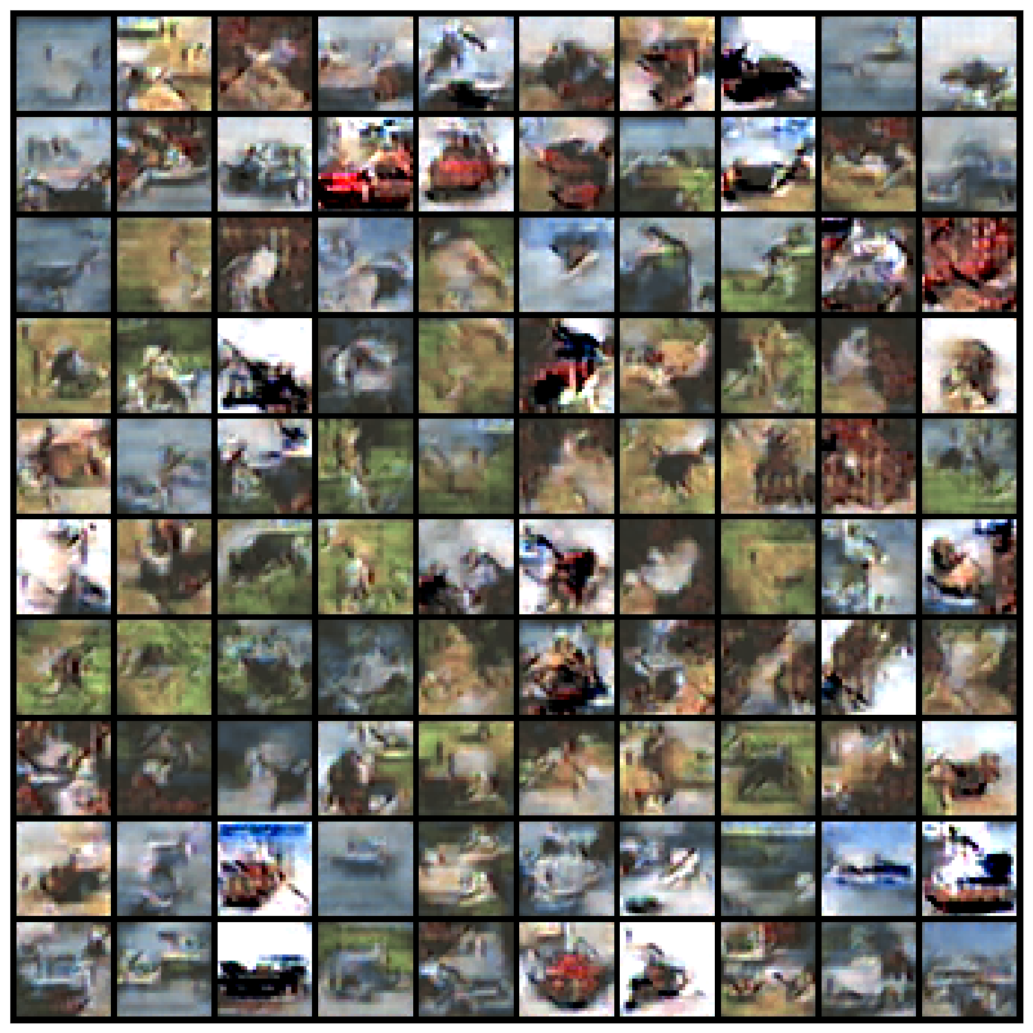
Low AUM (Hard) data

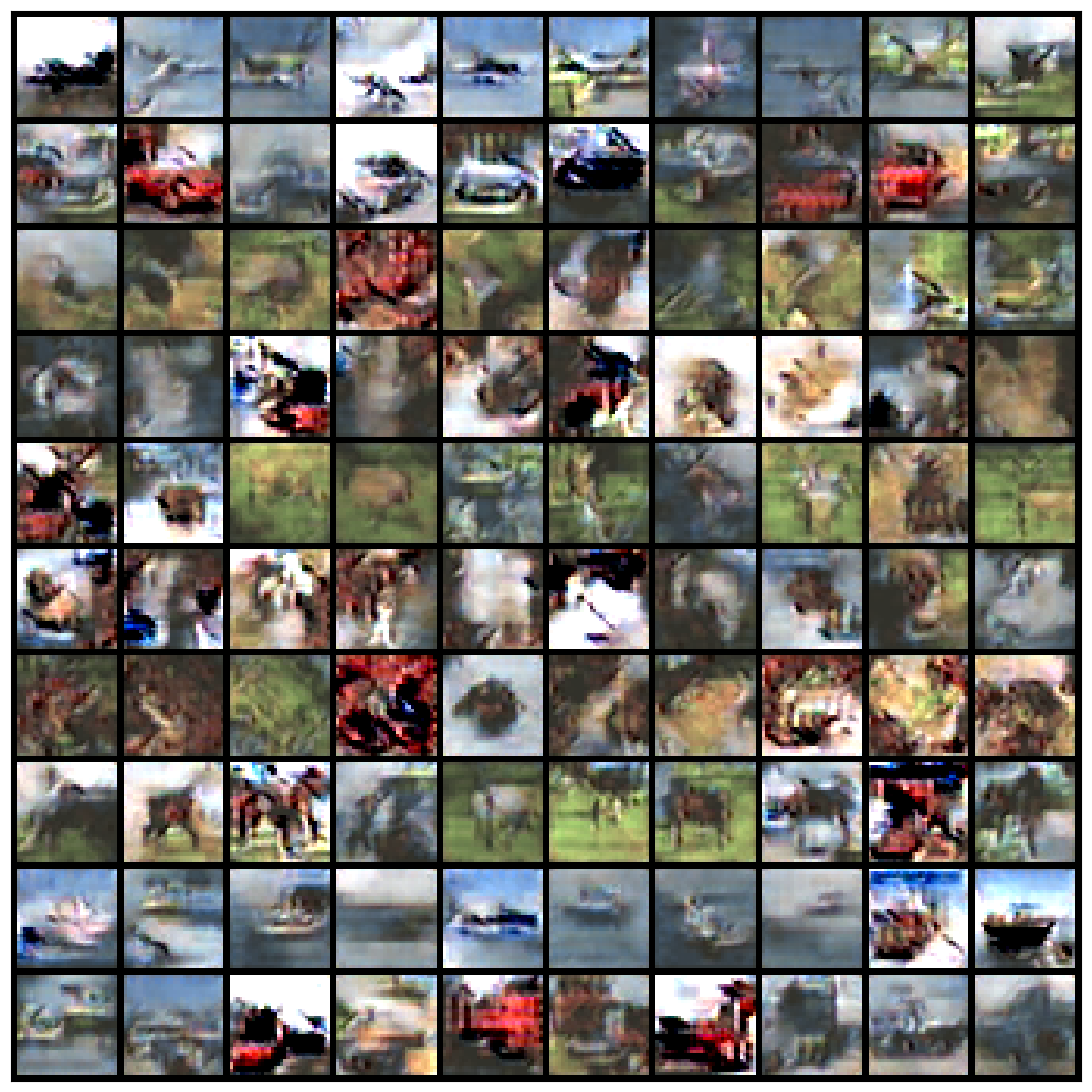
Randomly selected data

Figure 9: Images generated by a CIFAR10 HMN with 1.1IPC storage budget. Images in each row are from the same class.

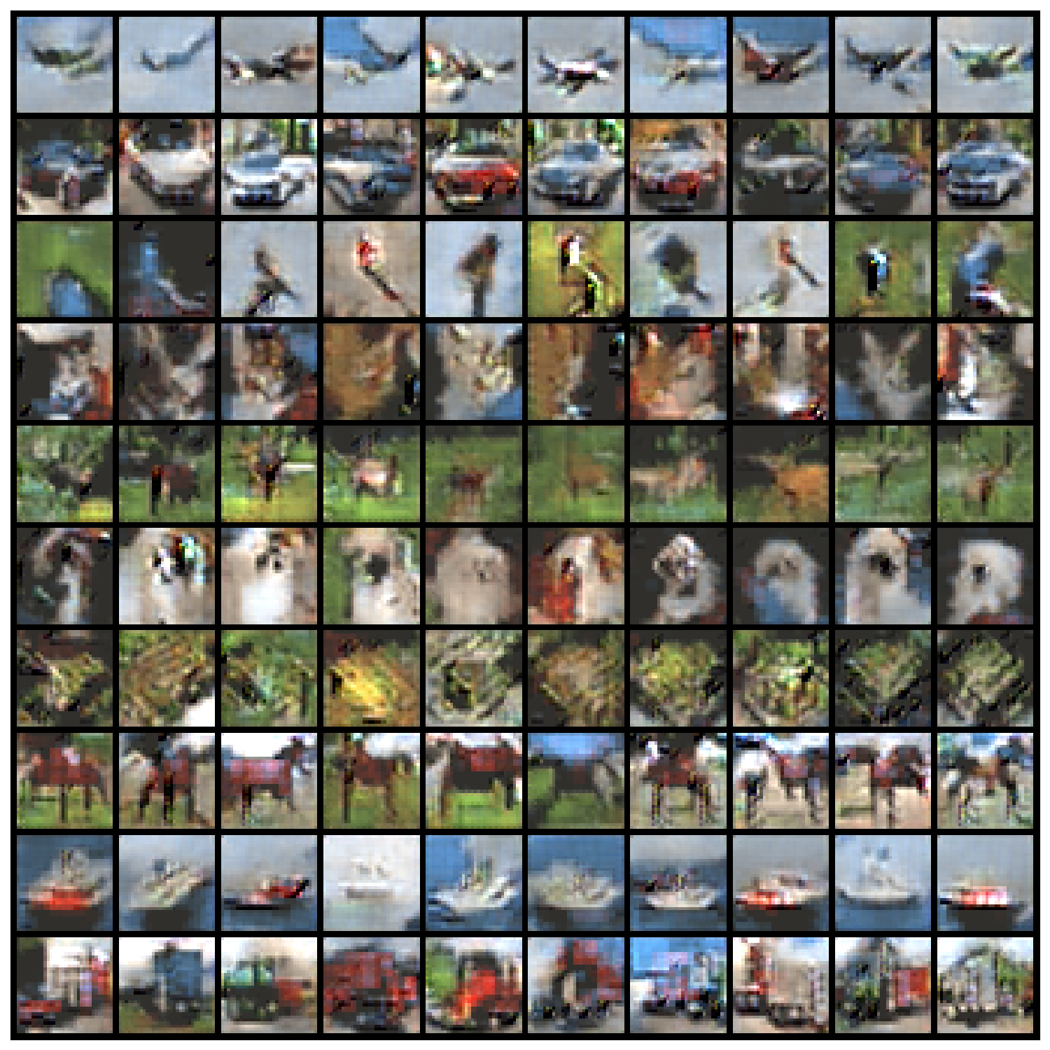
High AUM (Easy) data

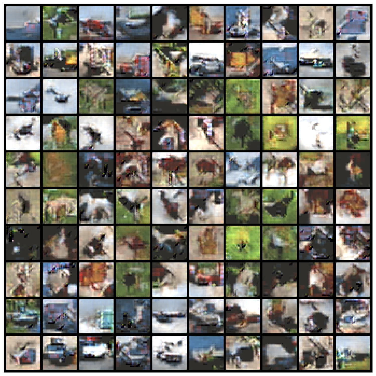
Low AUM (Hard) data

Randomly selected data

Figure 10: Images generated by a CIFAR10 HMN with 11IPC storage budget. Images in each row are from the same class.

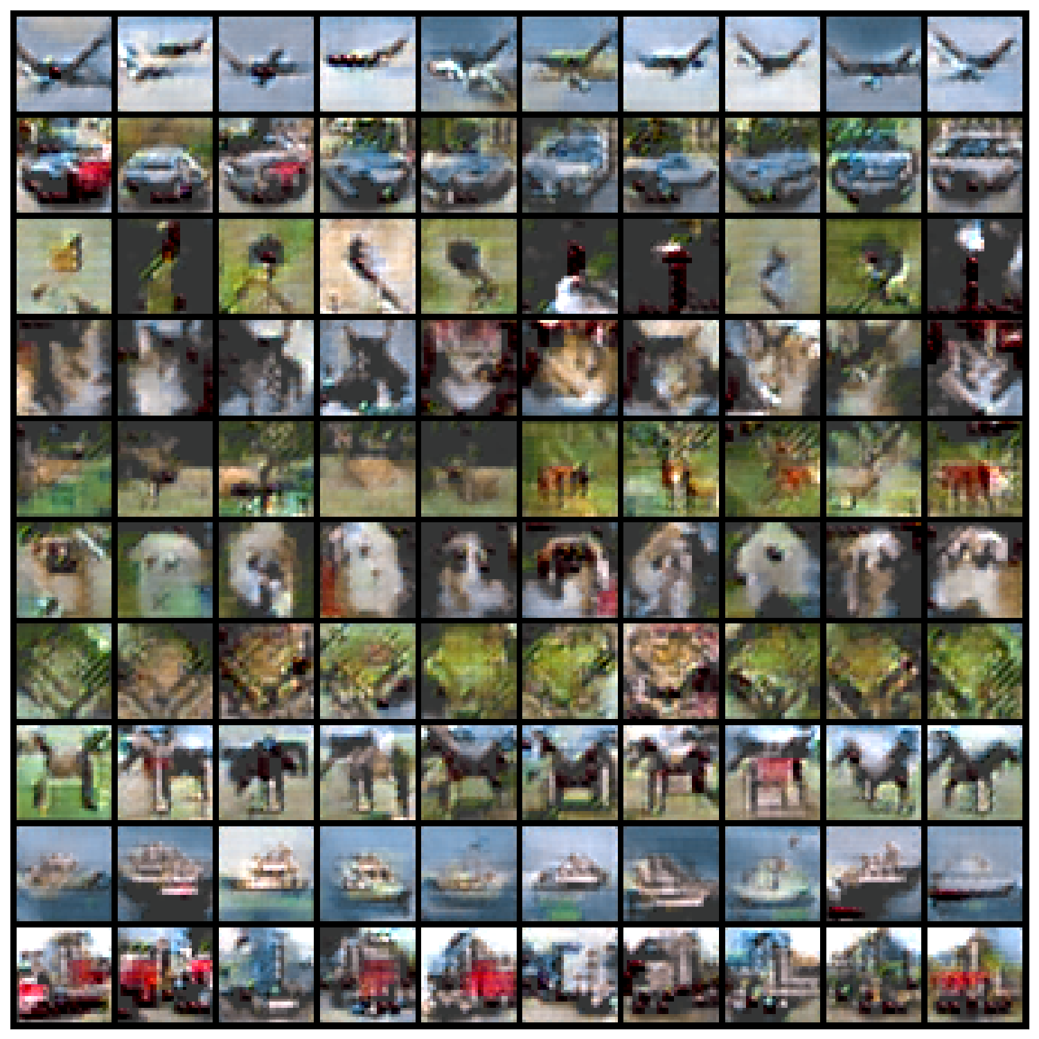
High AUM (Easy) data

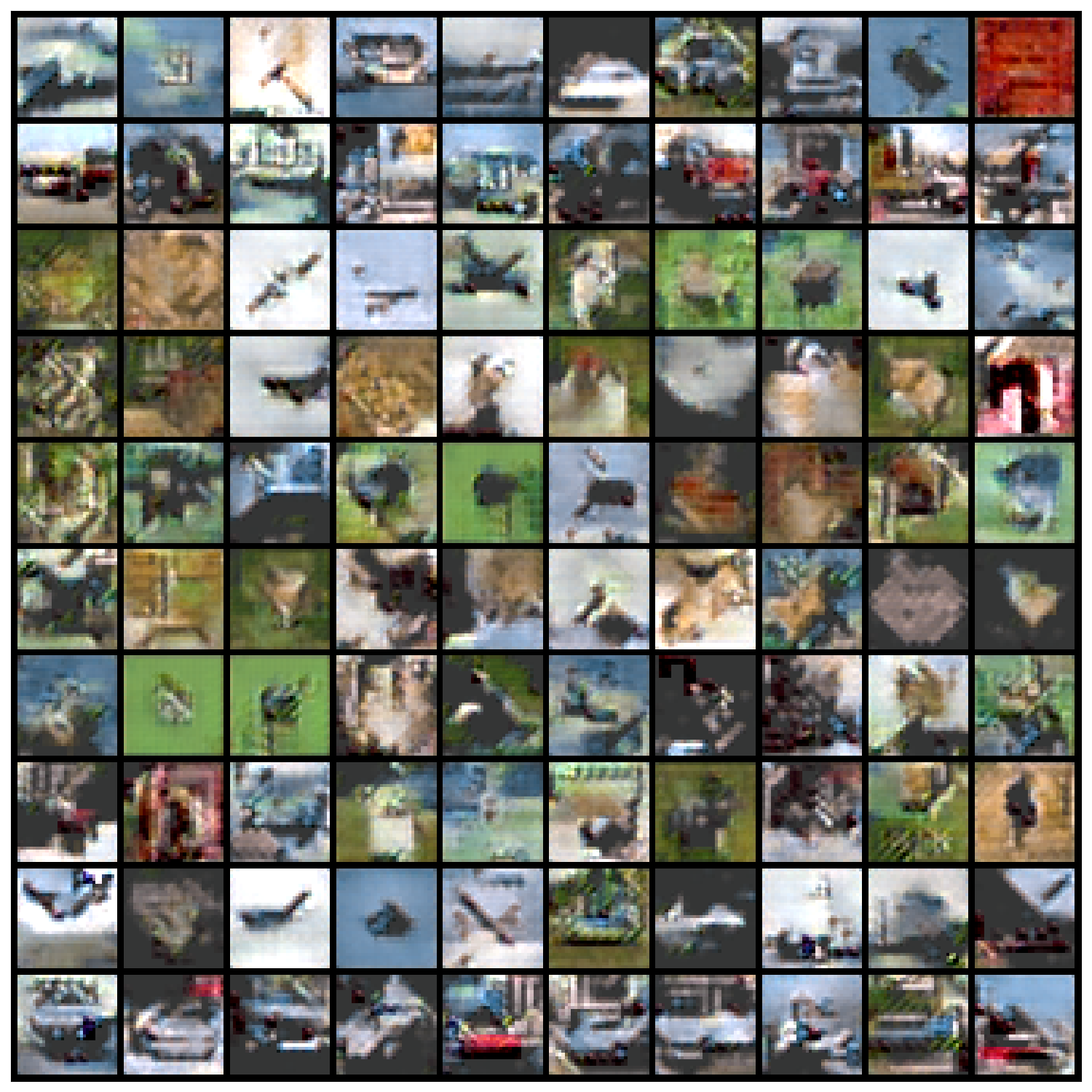
Low AUM (Hard) data

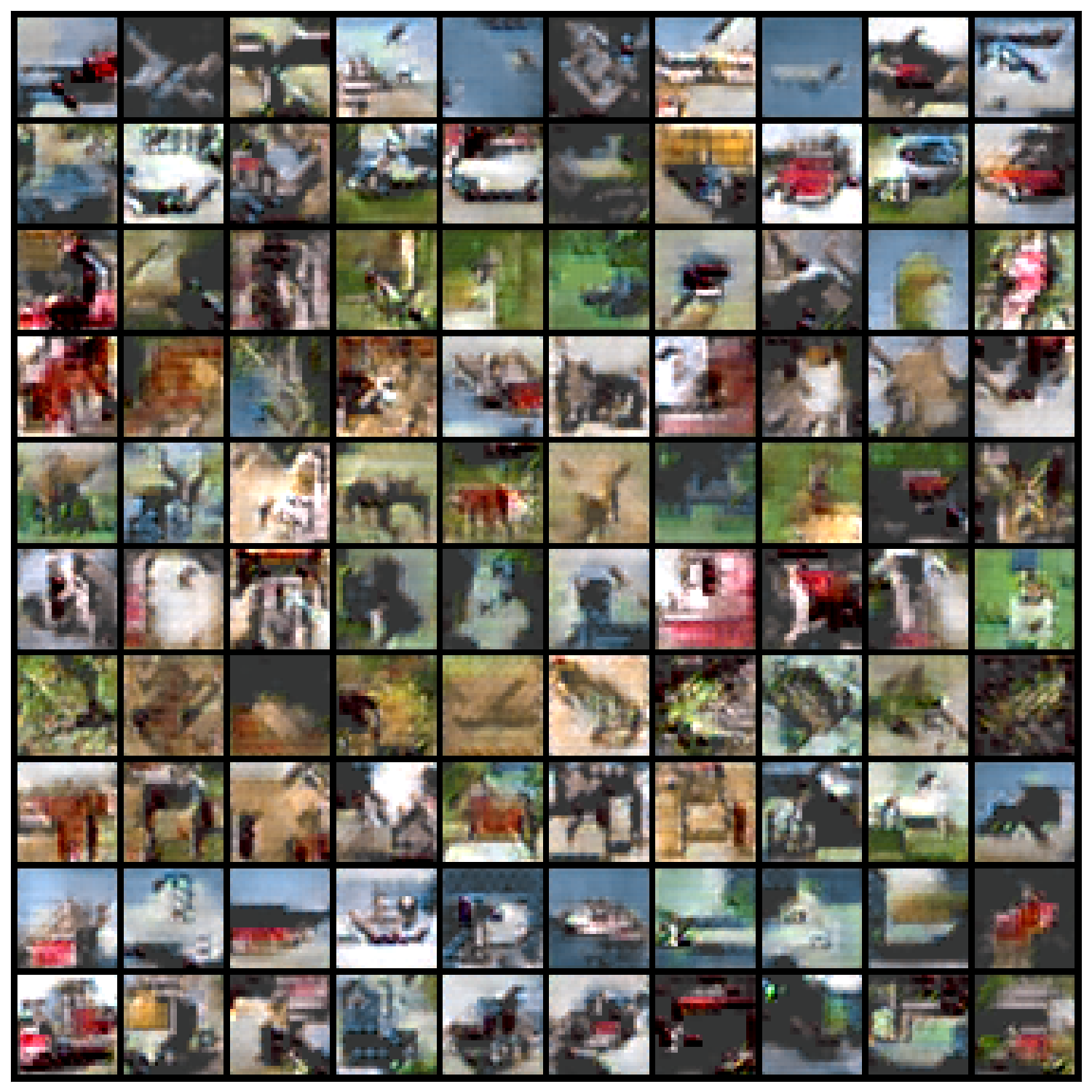
Randomly selected data

Figure 11: Images generated by a CIFAR10 HMN with 55IPC storage budget. Images in each row are from the same class.

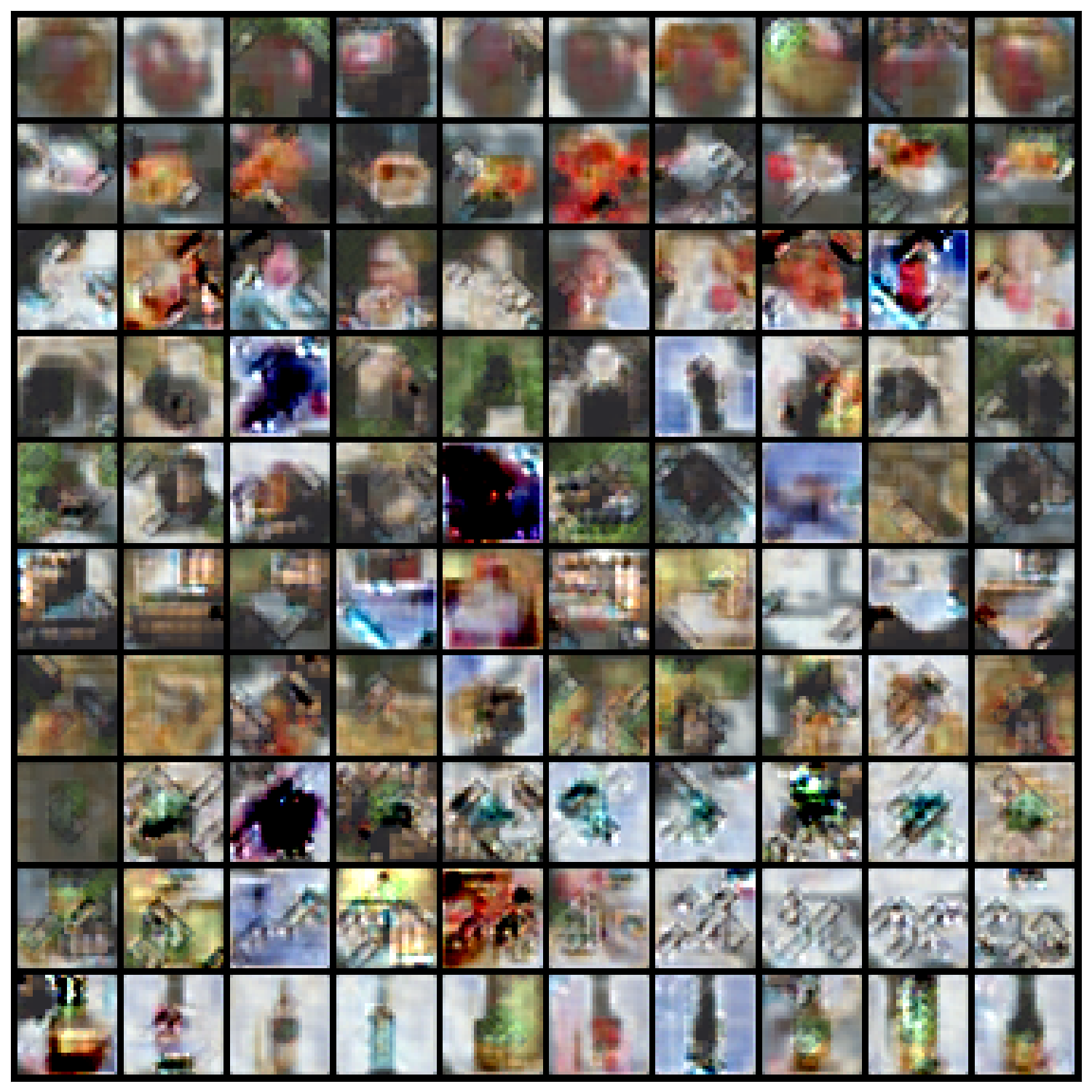
High AUM (Easy) data

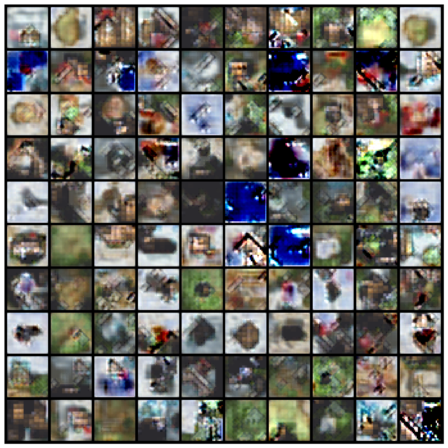
Low AUM (Hard) data

Randomly selected data

Figure 12: Images generated by a CIFAR100 HMN with 1.1IPC storage budget. Images in each row are from the same class. We only visualize 10 classes with the smallest class number in the dataset.

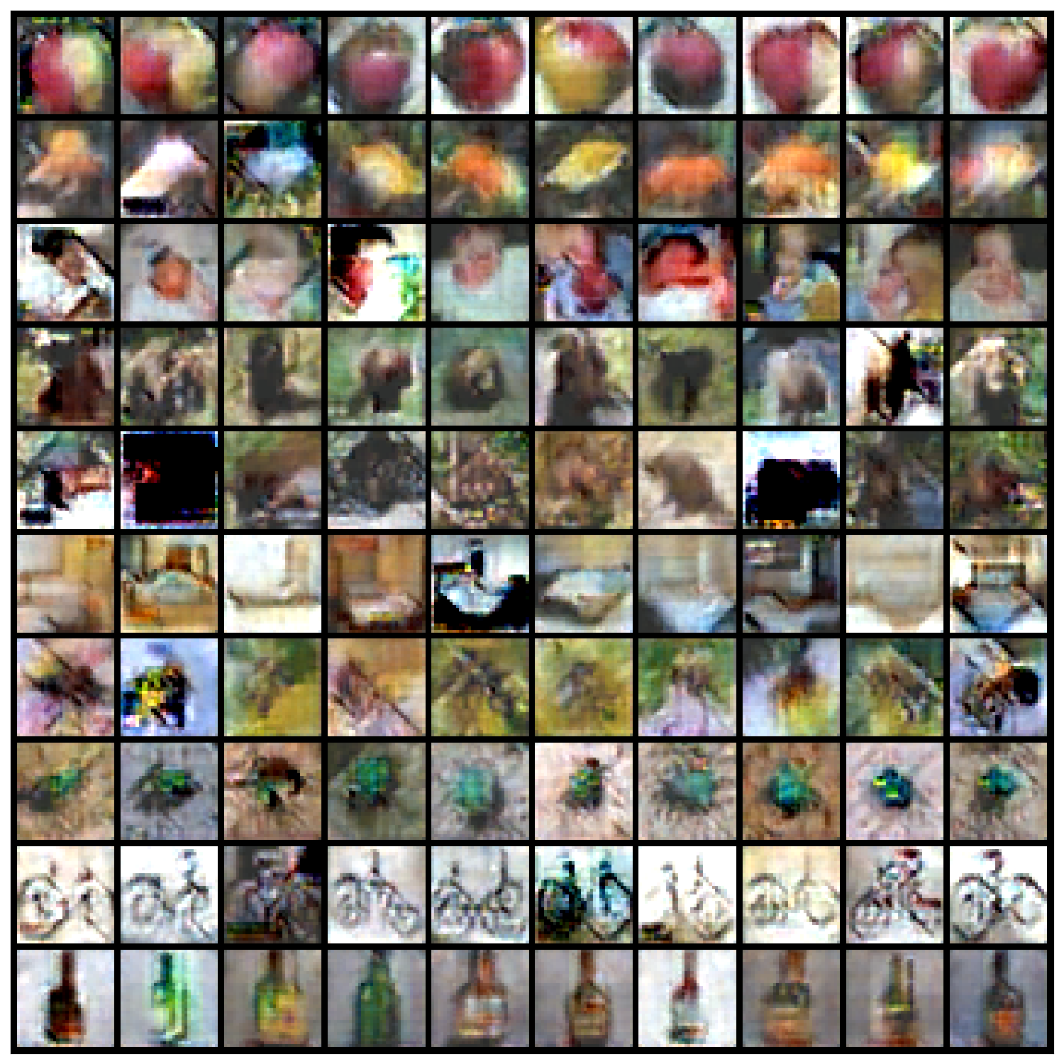
High AUM (Easy) data

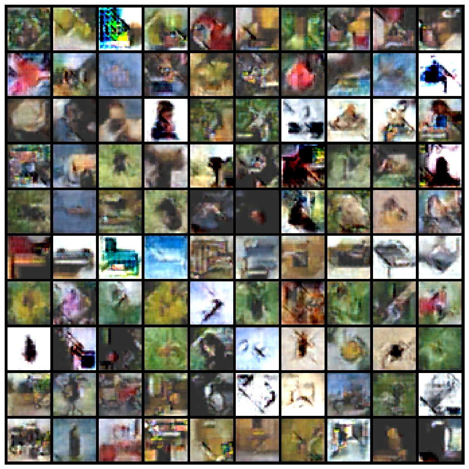
Low AUM (Hard) data

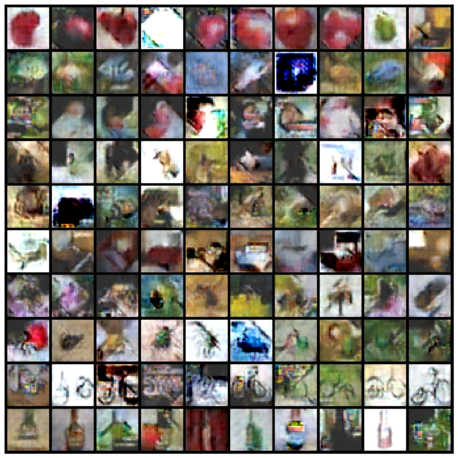
Randomly selected data

Figure 13: Images generated by a CIFAR100 HMN with 11IPC storage budget. Images in each row are from the same class. We only visualize 10 classes with the smallest class number in the dataset.

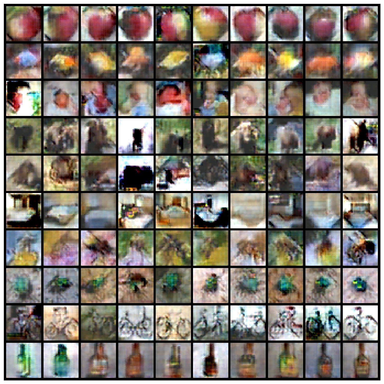
High AUM (Easy) data

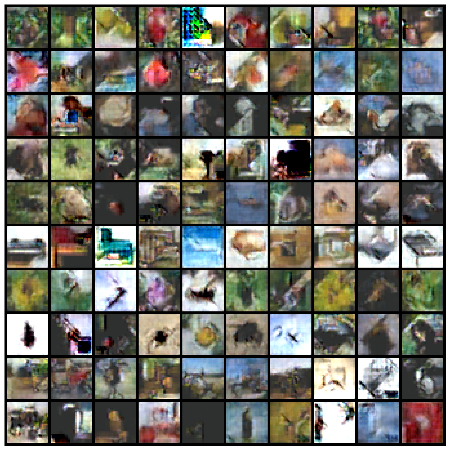
Low AUM (Hard) data

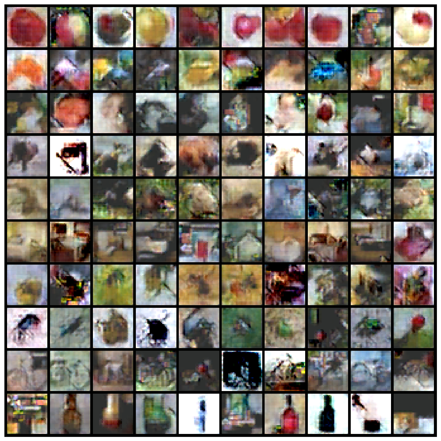
Randomly selected data

Figure 14: Images generated by a CIFAR100 HMN with 55IPC storage budget. Images in each row are from the same class. We only visualize 10 classes with the smallest class number in the dataset.

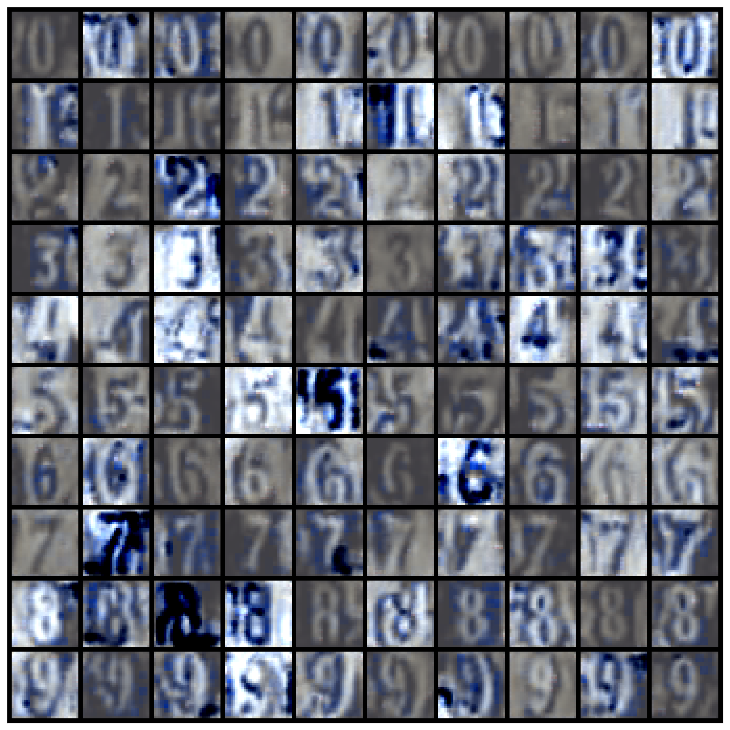
High AUM (Easy) data

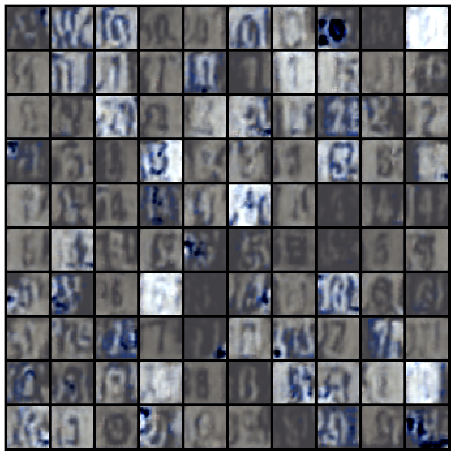
Low AUM (Hard) data

Randomly selected data

Figure 15: Images generated by an SVHN HMN with 1.1IPC storage budget. Images in each row are from the same class. Images with a low aum value are not well-aligned with its label and can be harmful for the training.

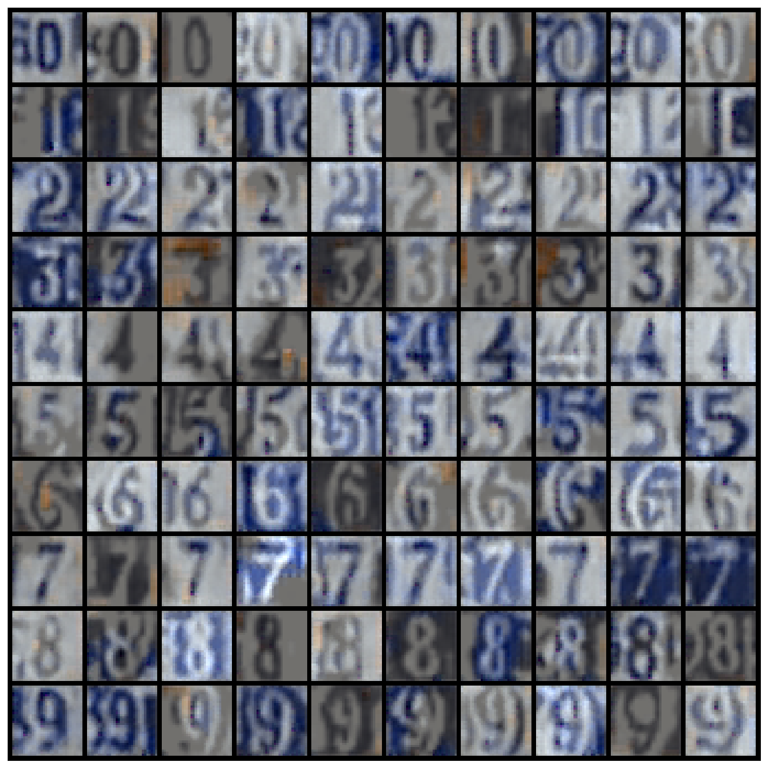
High AUM (Easy) data

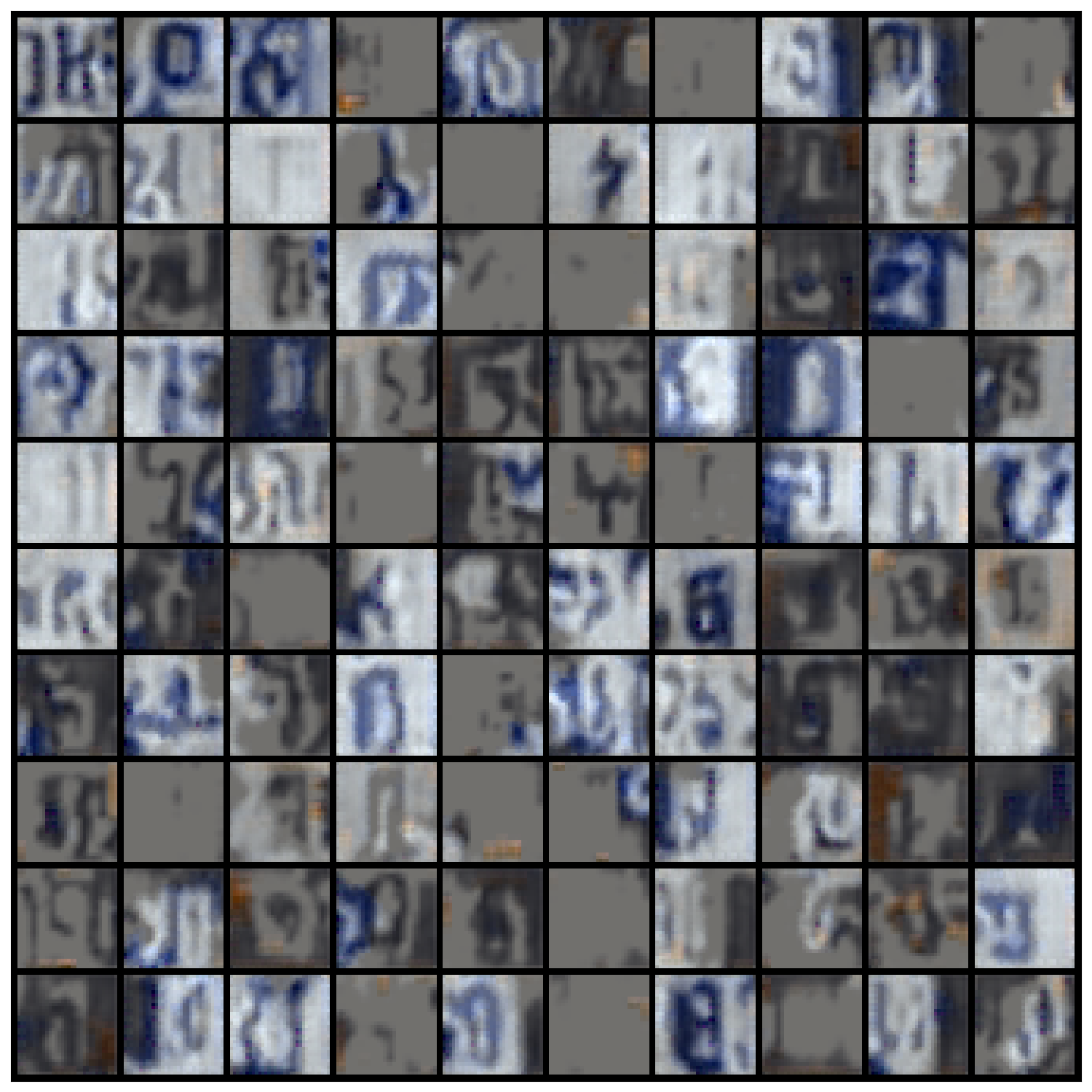
Low AUM (Hard) data

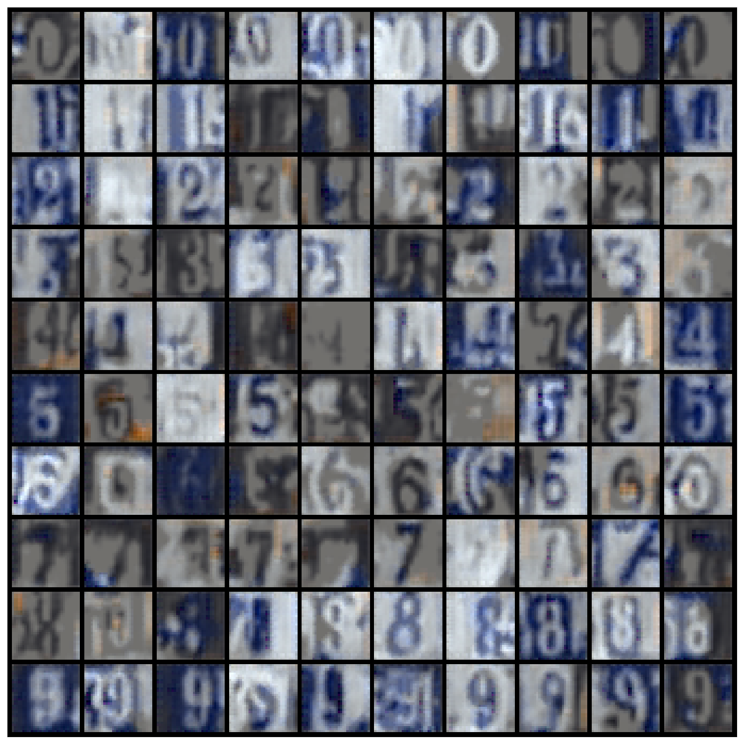
Randomly selected data

Figure 16: Images generated by an SVHN HMN with 11IPC storage budget. Images in each row are from the same class.

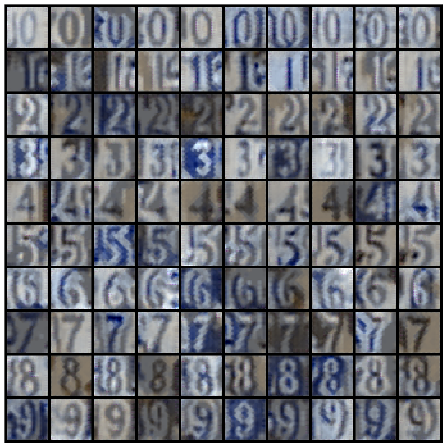
High AUM (Easy) data

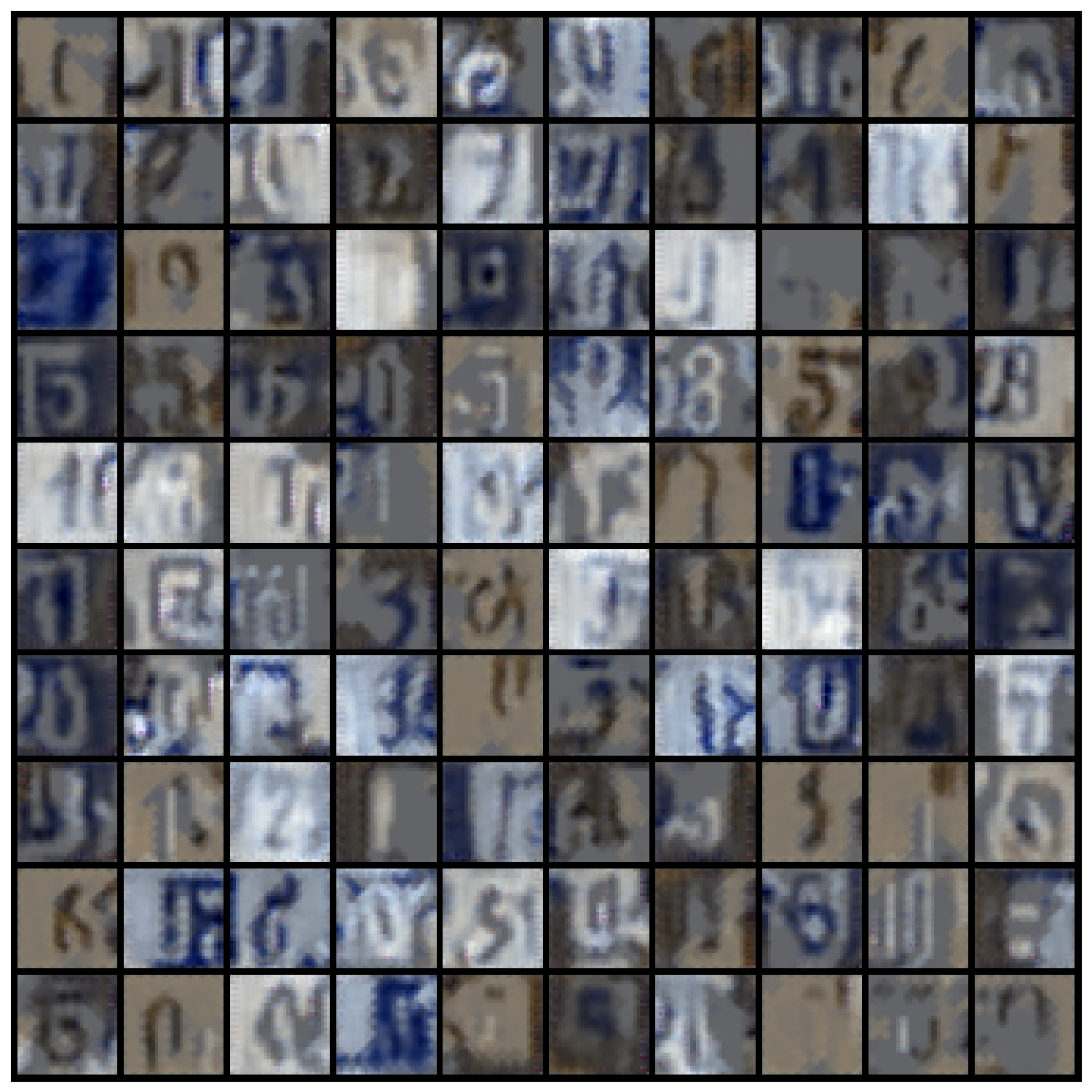
Low AUM (Hard) data

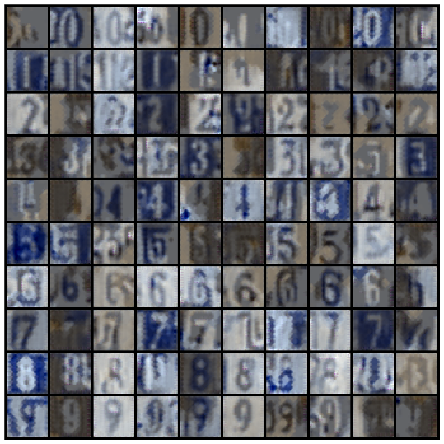
Randomly selected data

Figure 17: Images generated by an SVHN HMN with 55IPC storage budget. Images in each row are from the same class.

References

- Bang et al. (2021) Jihwan Bang, Heesu Kim, YoungJoon Yoo, Jung-Woo Ha, and Jonghyun Choi. Rainbow memory: Continual learning with a memory of diverse samples. In Proceedings of the IEEE/CVF Conference on Computer Vision and Pattern Recognition, pp. 8218–8227, 2021.
- Bartoldson et al. (2023) Brian R Bartoldson, Bhavya Kailkhura, and Davis Blalock. Compute-efficient deep learning: Algorithmic trends and opportunities. Journal of Machine Learning Research, 24:1–77, 2023.
- Brock et al. (2017) Andrew Brock, Theodore Lim, James Millar Ritchie, and Nicholas J Weston. Neural photo editing with introspective adversarial networks. In 5th International Conference on Learning Representations 2017, 2017.
- Cazenavette et al. (2022) George Cazenavette, Tongzhou Wang, Antonio Torralba, Alexei A Efros, and Jun-Yan Zhu. Dataset distillation by matching training trajectories. In Proceedings of the IEEE/CVF Conference on Computer Vision and Pattern Recognition, pp. 4750–4759, 2022.
- Cazenavette et al. (2023) George Cazenavette, Tongzhou Wang, Antonio Torralba, Alexei A Efros, and Jun-Yan Zhu. Generalizing dataset distillation via deep generative prior. In Proceedings of the IEEE Conference on Computer Vision and Pattern Recognition (CVPR), 2023.
- Chai et al. (2021a) Lucy Chai, Jonas Wulff, and Phillip Isola. Using latent space regression to analyze and leverage compositionality in gans. In International Conference on Learning Representations, 2021a.
- Chai et al. (2021b) Lucy Chai, Jun-Yan Zhu, Eli Shechtman, Phillip Isola, and Richard Zhang. Ensembling with deep generative views. In Proceedings of the IEEE/CVF Conference on Computer Vision and Pattern Recognition, pp. 14997–15007, 2021b.
- Chaudhry et al. (2019) Arslan Chaudhry, Marcus Rohrbach, Mohamed Elhoseiny, Thalaiyasingam Ajanthan, Puneet K Dokania, Philip HS Torr, and Marc’Aurelio Ranzato. On tiny episodic memories in continual learning. arXiv preprint arXiv:1902.10486, 2019.
- Coleman et al. (2019) Cody Coleman, Christopher Yeh, Stephen Mussmann, Baharan Mirzasoleiman, Peter Bailis, Percy Liang, Jure Leskovec, and Matei Zaharia. Selection via proxy: Efficient data selection for deep learning. In International Conference on Learning Representations, 2019.
- Cui et al. (2022) Justin Cui, Ruochen Wang, Si Si, and Cho-Jui Hsieh. Dc-bench: Dataset condensation benchmark. In Thirty-sixth Conference on Neural Information Processing Systems Datasets and Benchmarks Track, 2022.
- Cui et al. (2023) Justin Cui, Ruochen Wang, Si Si, and Cho-Jui Hsieh. Scaling up dataset distillation to imagenet-1k with constant memory. In International Conference on Machine Learning, pp. 6565–6590. PMLR, 2023.
- Deng et al. (2009) Jia Deng, Wei Dong, Richard Socher, Li-Jia Li, Kai Li, and Li Fei-Fei. Imagenet: A large-scale hierarchical image database. In 2009 IEEE conference on computer vision and pattern recognition, pp. 248–255. Ieee, 2009.
- Deng & Russakovsky (2022) Zhiwei Deng and Olga Russakovsky. Remember the past: Distilling datasets into addressable memories for neural networks. In Advances in Neural Information Processing Systems, 2022.
- Du et al. (2022) Jiawei Du, Yidi Jiang, Vincent TF Tan, Joey Tianyi Zhou, and Haizhou Li. Minimizing the accumulated trajectory error to improve dataset distillation. arXiv preprint arXiv:2211.11004, 2022.
- Jiang et al. (2022) Zixuan Jiang, Jiaqi Gu, Mingjie Liu, and David Z Pan. Delving into effective gradient matching for dataset condensation. arXiv preprint arXiv:2208.00311, 2022.
- Kim et al. (2022) Jang-Hyun Kim, Jinuk Kim, Seong Joon Oh, Sangdoo Yun, Hwanjun Song, Joonhyun Jeong, Jung-Woo Ha, and Hyun Oh Song. Dataset condensation via efficient synthetic-data parameterization. In International Conference on Machine Learning, pp. 11102–11118. PMLR, 2022.
- Krizhevsky et al. (2009) Alex Krizhevsky, Geoffrey Hinton, et al. Learning multiple layers of features from tiny images. Technical report, Citeseer, 2009.
- Lee et al. (2022) Saehyung Lee, Sanghyuk Chun, Sangwon Jung, Sangdoo Yun, and Sungroh Yoon. Dataset condensation with contrastive signals. In International Conference on Machine Learning, pp. 12352–12364. PMLR, 2022.
- Li et al. (2023) Yize Li, Pu Zhao, Xue Lin, Bhavya Kailkhura, and Ryan Goldhahn. Less is more: Data pruning for faster adversarial training. arXiv preprint arXiv:2302.12366, 2023.
- Li & Hoiem (2018) Zhizhong Li and Derek Hoiem. Learning without forgetting. IEEE Transactions on Pattern Analysis and Machine Intelligence, 40(12):2935–2947, 2018. doi: 10.1109/TPAMI.2017.2773081.
- Liu et al. (2022) Songhua Liu, Kai Wang, Xingyi Yang, Jingwen Ye, and Xinchao Wang. Dataset distillation via factorization. In Advances in Neural Information Processing Systems, 2022.
- Liu et al. (2023) Yanqing Liu, Jianyang Gu, Kai Wang, Zheng Zhu, Wei Jiang, and Yang You. Dream: Efficient dataset distillation by representative matching. arXiv preprint arXiv:2302.14416, 2023.
- Loshchilov & Hutter (2017) Ilya Loshchilov and Frank Hutter. Sgdr: Stochastic gradient descent with warm restarts. In ICLR, 2017.
- Netzer et al. (2011) Yuval Netzer, Tao Wang, Adam Coates, Alessandro Bissacco, Bo Wu, and Andrew Y. Ng. Reading digits in natural images with unsupervised feature learning. In NIPS Workshop on Deep Learning and Unsupervised Feature Learning 2011, 2011. URL http://ufldl.stanford.edu/housenumbers/nips2011_housenumbers.pdf.
- Nguyen et al. (2020) Timothy Nguyen, Zhourong Chen, and Jaehoon Lee. Dataset meta-learning from kernel ridge-regression. In International Conference on Learning Representations, 2020.
- Nguyen et al. (2021) Timothy Nguyen, Roman Novak, Lechao Xiao, and Jaehoon Lee. Dataset distillation with infinitely wide convolutional networks. Advances in Neural Information Processing Systems, 34:5186–5198, 2021.
- Paul et al. (2021) Mansheej Paul, Surya Ganguli, and Gintare Karolina Dziugaite. Deep learning on a data diet: Finding important examples early in training. Advances in Neural Information Processing Systems, 34, 2021.
- Pleiss et al. (2020) Geoff Pleiss, Tianyi Zhang, Ethan Elenberg, and Kilian Q Weinberger. Identifying mislabeled data using the area under the margin ranking. Advances in Neural Information Processing Systems, 33:17044–17056, 2020.
- Rebuffi et al. (2017a) Sylvestre-Alvise Rebuffi, Alexander Kolesnikov, Georg Sperl, and Christoph H. Lampert. icarl: Incremental classifier and representation learning. In Proceedings of the IEEE Conference on Computer Vision and Pattern Recognition (CVPR), July 2017a.
- Rebuffi et al. (2017b) Sylvestre-Alvise Rebuffi, Alexander Kolesnikov, Georg Sperl, and Christoph H Lampert. icarl: Incremental classifier and representation learning. In Proceedings of the IEEE conference on Computer Vision and Pattern Recognition, pp. 2001–2010, 2017b.
- Rosasco et al. (2022) Andrea Rosasco, Antonio Carta, Andrea Cossu, Vincenzo Lomonaco, and Davide Bacciu. Distilled replay: Overcoming forgetting through synthetic samples. In Continual Semi-Supervised Learning: First International Workshop, CSSL 2021, Virtual Event, August 19–20, 2021, Revised Selected Papers, pp. 104–117. Springer, 2022.
- Sangermano et al. (2022) Mattia Sangermano, Antonio Carta, Andrea Cossu, and Davide Bacciu. Sample condensation in online continual learning. In 2022 International Joint Conference on Neural Networks (IJCNN), pp. 01–08. IEEE, 2022.
- Sener & Savarese (2017) Ozan Sener and Silvio Savarese. Active learning for convolutional neural networks: A core-set approach. arXiv preprint arXiv:1708.00489, 2017.
- Shin et al. (2023) Seungjae Shin, Heesun Bae, Donghyeok Shin, Weonyoung Joo, and Il-Chul Moon. Loss-curvature matching for dataset selection and condensation. In International Conference on Artificial Intelligence and Statistics, pp. 8606–8628. PMLR, 2023.
- Song et al. (2022) Rui Song, Dai Liu, Dave Zhenyu Chen, Andreas Festag, Carsten Trinitis, Martin Schulz, and Alois Knoll. Federated learning via decentralized dataset distillation in resource-constrained edge environments. arXiv preprint arXiv:2208.11311, 2022.
- Sorscher et al. (2022) Ben Sorscher, Robert Geirhos, Shashank Shekhar, Surya Ganguli, and Ari S Morcos. Beyond neural scaling laws: beating power law scaling via data pruning. arXiv preprint arXiv:2206.14486, 2022.
- Toneva et al. (2018) Mariya Toneva, Alessandro Sordoni, Remi Tachet des Combes, Adam Trischler, Yoshua Bengio, and Geoffrey J Gordon. An empirical study of example forgetting during deep neural network learning. In International Conference on Learning Representations, 2018.
- Wang et al. (2022) Kai Wang, Bo Zhao, Xiangyu Peng, Zheng Zhu, Shuo Yang, Shuo Wang, Guan Huang, Hakan Bilen, Xinchao Wang, and Yang You. Cafe: Learning to condense dataset by aligning features. In Proceedings of the IEEE/CVF Conference on Computer Vision and Pattern Recognition, pp. 12196–12205, 2022.
- Wang et al. (2018) Tongzhou Wang, Jun-Yan Zhu, Antonio Torralba, and Alexei A Efros. Dataset distillation. arXiv preprint arXiv:1811.10959, 2018.
- Xia et al. (2023) Xiaobo Xia, Jiale Liu, Jun Yu, Xu Shen, Bo Han, and Tongliang Liu. Moderate coreset: A universal method of data selection for real-world data-efficient deep learning. In International Conference on Learning Representations, 2023.
- Xiong et al. (2022) Yuanhao Xiong, Ruochen Wang, Minhao Cheng, Felix Yu, and Cho-Jui Hsieh. Feddm: Iterative distribution matching for communication-efficient federated learning. arXiv preprint arXiv:2207.09653, 2022.
- Zhao & Bilen (2021) Bo Zhao and Hakan Bilen. Dataset condensation with differentiable siamese augmentation. In International Conference on Machine Learning, pp. 12674–12685. PMLR, 2021.
- Zhao & Bilen (2022) Bo Zhao and Hakan Bilen. Synthesizing informative training samples with gan. In NeurIPS 2022 Workshop on Synthetic Data for Empowering ML Research, 2022.
- Zhao & Bilen (2023a) Bo Zhao and Hakan Bilen. Dataset condensation with distribution matching. In Proceedings of the IEEE/CVF Winter Conference on Applications of Computer Vision, pp. 6514–6523, 2023a.
- Zhao & Bilen (2023b) Bo Zhao and Hakan Bilen. Dataset condensation with distribution matching. In Proceedings of the IEEE/CVF Winter Conference on Applications of Computer Vision, pp. 6514–6523, 2023b.
- Zhao et al. (2021) Bo Zhao, Konda Reddy Mopuri, and Hakan Bilen. Dataset condensation with gradient matching. In Ninth International Conference on Learning Representations 2021, 2021.
- Zheng et al. (2020) Haizhong Zheng, Ziqi Zhang, Juncheng Gu, Honglak Lee, and Atul Prakash. Efficient adversarial training with transferable adversarial examples. In Proceedings of the IEEE/CVF Conference on Computer Vision and Pattern Recognition, pp. 1181–1190, 2020.
- Zheng et al. (2023) Haizhong Zheng, Rui Liu, Fan Lai, and Atul Prakash. Coverage-centric coreset selection for high pruning rates. In International Conference on Learning Representations 2023, 2023.