Sample-Driven Federated Learning for Energy-Efficient and Real-Time IoT Sensing

Abstract

In the domain of Federated Learning (FL) systems, recent cutting-edge methods heavily rely on ideal conditions convergence analysis. Specifically, these approaches assume that the training datasets on IoT devices possess similar attributes to the global data distribution. However, this approach fails to capture the full spectrum of data characteristics in real-time sensing FL systems. In order to overcome this limitation, we suggest a new approach system specifically designed for IoT networks with real-time sensing capabilities. Our approach takes into account the generalization gap due to the user’s data sampling process. By effectively controlling this sampling process, we can mitigate the overfitting issue and improve overall accuracy. In particular, We first formulate an optimization problem that harnesses the sampling process to concurrently reduce overfitting while maximizing accuracy. In pursuit of this objective, our surrogate optimization problem is adept at handling energy efficiency while optimizing the accuracy with high generalization. To solve the optimization problem with high complexity, we introduce an online reinforcement learning algorithm, named Sample-driven Control for Federated Learning (SCFL) built on the Soft Actor-Critic (A2C) framework. This enables the agent to dynamically adapt and find the global optima even in changing environments. By leveraging the capabilities of SCFL, our system offers a promising solution for resource allocation in FL systems with real-time sensing capabilities.

I Introduction

Federated Learning (FL) [1, 2] is a distributed learning algorithm that is widely utilized in Internet-of-Things (IoT) and wireless systems [3, 4, 5]. FL allows IoT devices to construct a collaborative learning model by locally training their collected data [6, 7, 8]. Instead of sharing the training data, the devices in FL can collaboratively perform a learning task by only uploading a local learning model to the aggregation server at the network edge [9]. As such, FL systems could improve wireless systems by addressing privacy constraints and limited data transfer bandwidth. Because it is not feasible for all the devices to transmit all of the data to a data center, which can use the collected data to implement centralized machine learning algorithms for data analysis and inference [10, 11]. Despite the considerable successes of FL, there are still technical issues, i.e., communication efficiency [12] and non-independent and identically distributed data (non-IID) [13], while deploying FL in the IoT networks, which need to be addressed.

I-A Example and Motivation

Recent studies in [14, 15, 16, 17] explored energy consumption in both local computation and wireless transmission; however, these studies derive the convergence rate according to the gradient descent on the training dataset, i.e., distributed device-specific data, without deep understanding of the FL performance on test dataset (the ideal global data). Hence, when employing FL in a real-time sensing (RTS) system, having sampling times that are too closely spaced can result in a high correlation among consecutive data. This correlation may give rise to two potential issues.

1. Bias in Gradient Descent: Correlated datasets may cause bias during the gradient descent process, causing the model to favor specific sets of unbalanced data [18].

2. Vanishing Gradient: Due to a high correlation with previously sampled data, the gradient of the new dataset may become too small, leading to the vanishing gradient problem [19]. This issue can hinder effective learning and slow down or halt the model’s training process. To illustrate this phenomenon, we consider the following example of RTS.

Example 1.

We have three images of a kitten running towards the security camera at different sampling times in Fig. 2. The security camera is trained for the object detection task. To fully comprehend the influence of real-time sampling on the data collected from security cameras, we consider the two descriptions for the difference of the images in three instances.

• Fig. 2(i) at time $t$ depicts the kitten at a distance from the camera, blurred and difficult to identify. After a very short time interval $\tau_{u}$, the cat in Fig. 2(ii) has almost the same detail and size as it is in Fig. 2(i)

• In Fig. 2(iii) at time $t+k\times\tau_{u}$, the kitten is noticeably different from itself in Fig. (i). As a result, the information about the kitten in these two figures bring is significantly different.

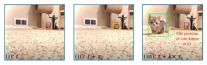
Figure 1: Illustration of how sampling delay impacts overfitting in AI.

From Example 1, it is evident that when using a short sampling time for the RTS setting in the FL system, there is little difference between the images captured at close and far distances of the kitten. This results in the Artificial Intelligence (AI) model struggling to identify the kitten when it is close to the camera, as it mainly becomes proficient at recognizing distant instances. Consequently, the system faces challenges in processing redundant data, leading to prolonged processing times and a higher risk of overfitting.

To address this issue in the RTS system, one straightforward approach is to increase the sampling interval between two samples. However, doing so necessitates careful consideration of sampling energy efficiency. Skipping more samples from sensing devices (i.e., surveillance cameras and sensors) results in increased energy consumption by the FL system and longer wait times to gather sufficient data for the training process. Therefore, a balance must be struck to optimize the sampling interval while efficiently utilizing energy and time resources. Moreover, to enhance AI training, sampling data with diverse information becomes crucial, especially considering the limited data storage capacity of distributed clients.

I-B Contributions

Upon acknowledging the severity of the issue identified in the aforementioned studies concerning the use of an ideal dataset, we have devised a solution in the form of Sample-driven Control for FL (SCFL) in real-time sensing. This approach is specifically designed to address the challenges arising from the generalization gap. To be more specific, the generalization gap is a fundamental concept that quantifies the disparity in the model’s performance between two distinct datasets. By drawing upon this concept, we can address the problem of AI model overfitting to non-ideal datasets, as opposed to assuming the data is ideal. Furthermore, by incorporating the generalization gap, we can establish a connection between the convergence of the training model and other data-related factors (e.g., data sampling interval). Consequently, implementing sample-driven control mechanisms improves the performance and reliability of FL systems while guaranteeing network performance in real-time sensing tasks.

In this paper, our focus lies on the resource allocation for multiple users within a considered IoT network. Specifically, we aim to minimize the overall energy consumption during the deployment of FL by employing sample-driven control with real-time sensing. To achieve this, we propose a new model called SCFL, which leverages the concept of the generalization gap and utilizes a Deep Reinforcement Learning (DRL) algorithm. In SCFL, a set of real-time data is used for training to effectively control the sampling process within the FL system. The main objective of SCFL is to obtain optimal network settings along with data-sampling intervals to allocate computation and communication resources efficiently while guaranteeing the FL process convergence with high generalization. To the best of our knowledge, this is the first work that considers the AI performance on non-ideal datasets (e.g., dataset collected from RTS system). In summary, the key contributions of this paper can be summarized as follows:

• We take the generalization gap due to the user’s sampling into consideration. On that account, we find that by controlling the user’s sampling process, we can significantly reduce the overfitting phenomenon.

• We formulate a first-ever optimization problem that utilizes the sampling process that can reduce the overfitting phenomenon at the same time with high accuracy.

• To solve this problem, we introduce an online reinforcement learning algorithm by leveraging an advanced DRL algorithm called Soft Actor-Critic (A2C). Therefore, the learning agent can automatically find the optimal solution adaptively to the changes in the environment.

• We conduct intensive experiments to evaluate our proposed problem and sampling control algorithm.

I-C Paper Organization

The subsequent sections of this paper are structured as follows. In Section II, we present the system model and FL system model. Section III provides a comprehensive overview of our proposed SCFL approach, along with the problem formulation. In Section IV, we delve into the investigation of a DRL approach for SCFL. Experimental settings and results are discussed in Section V. Finally, in Section VI, we provide concluding remarks.

II System Model

We consider a network that consists of one edge server (ES) that is equipped with computing capabilities and serves $U$ users, denoted as $\mathcal{U}=\{1,2,\ldots,U\}$ (as shown in Fig. 2). Each user $u$ has a local dataset $\mathcal{D}_{u}$ with $D_{u}$ data samples. For each dataset $\mathcal{D}_{u}=\{x_{u,i},y_{u,i}\}^{D_{u}}_{i=1}$, $x_{u,i}\in\mathbb{R}^{d}$ is an input vector of user $u$ and $y_{u,i}$ is its corresponding output (e.g., the truth predict labeled by experts). The BS and all IoT devices of users cooperatively perform an FL algorithm over wireless networks for data analysis and inference. Hereinafter, the FL model that is trained by each user’s dataset is called the local FL model, while the FL model that is generated by aggregation algorithms at the ES (e.g., FedAvg [1], FedProx [20], SCAFFOLD [8]) is called the global FL model.

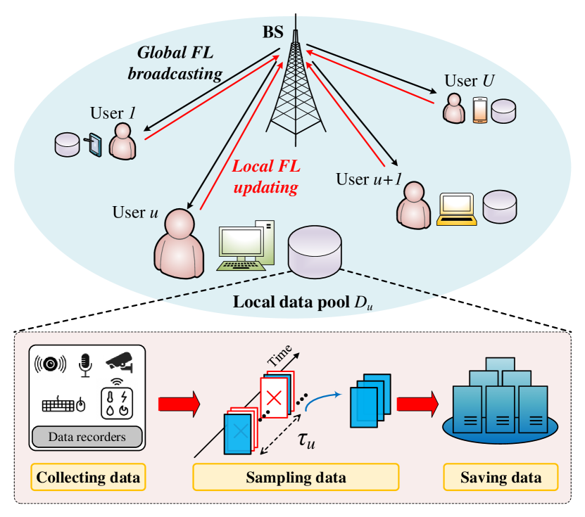
Figure 2: The architecture of our FL framework.

II-A Computation and Transmission Model

The FL cycle between the base station (BS) and the users in its service area consists of four steps: 1) Data sampling, which is performed at the user, with arbitrary sampling interval; 2) Local computation, which is performed at the user, with numerous local iterations; 3) Wireless communication (user sends local FL model after finishing and receiving parameters from BS); and 4) BS operation, which comprises aggregation and broadcasting.

II-A1 Local Sampling

User $u$ is equipped with real-time sensors to capture data for online AI learning. Each sensor possesses optimal sampling capabilities $\tau_{u}$ (e.g., the shortest possible time that a sensor can capture two consecutive data samples). Let’s denote $k_{u}$ as the number of sampling times skipped between two actual consecutive data points recorded by the sensor. The sensor consumes power $\mathcal{P}_{u}$ (Jules per sample) to capture each sampling data point. Thus, we can estimate the total sampling energy consumed by user $u$ as follows:

$$E_{u}^{\mathrm{S}}=k_{u}\mathcal{P}_{u}.$$ (1)

II-A2 Local Computation

The computation time required for data processing at user $u$ is defined as

$$t^{\textrm{comp}}_{u}=I_{u}\frac{C_{u}D_{u}}{f_{u}},\quad\forall u\in\mathcal{U},$$ (2)

where $I_{u}$ is the number of local iterations executed by each user $u$, $C_{u}$ [cycles/sample] and $f_{u}$ [Hz] is the number of CPU cycles needed to compute one sample data and the CPU frequency of user $u$, respectively. Denote by $\kappa$ the effective switching capacitance determined by the chip architecture. User $u$ needs the following energy consumption for local training [16]:

$$E_{u}^{\mathrm{C}}=\kappa I_{u}C_{u}D_{u}f_{u}^{2}.$$ (3)

II-A3 Wireless Communication

After local computation, all users employ frequency domain multiple access to submit their local FL model to the BS. The user $u$’s achievable rate is

$$r_{u}=b_{u}\log_{2}\left(1+\frac{g_{u}p_{u}}{n_{0}b_{u}}\right),\quad\forall u\in\mathcal{U},\sum^{U}_{u=1}b_{u}\leq B,$$ (4)

where $b_{u}$ is the user’s allocated bandwidth, $g_{u}$ is the channel gain of the wireless channel between user $u$ and the BS, $p_{u}$ is the average transmit power of user $u$, $n_{0}$ is the Gaussian noise power spectral density, and $B$ is the total bandwidth of FL system. Because the dimensions of the local FL model are fixed for all users, the data size required by each user is constant and expressed as $D_{0}$. We draw inspiration from the FL resource allocation algorithm concept introduced in [16]. Our objective is to manage the timeout for individual users denoted as $u$ by adjusting the coefficient $t_{u}^{\textrm{trans}}$. To upload data of size $D_{0}$ during transmission time $t_{u}^{\textrm{trans}}$, we hold the condition that $r_{u}t_{u}^{\textrm{trans}}\geq D_{0}$. To transfer data of size $D_{0}$ during a time length of $t_{u}^{\textrm{trans}}$, the user $u$’s transmit energy is

$$E^{T}_{u}=p_{u}t^{\textrm{trans}}_{u}.$$ (5)

II-A4 BS Operation

The BS receives the local parameters from all users in the global iteration and aggregates them for the global FL model at this stage. The BS transmits the global FL model to all users on the downlink. Because of the BS’s strong transmit power and the large bandwidth available for data broadcasting, the downstream time is disregarded compared to the uplink data transmission time. During this phase, the BS cannot access the user’s $\mathcal{D}_{u}$ dataset. This signifies that the FL algorithm’s privacy protection criterion protects the user’s privacy.

According to the aforementioned FL model system, each user’s energy consumption comprises both local computing energy $E^{C}_{u}$, sampling energy $E^{S}_{u}$ and wireless transmission energy $E^{T}_{u}$. The FL system implements a number of global communication rounds defined as $I_{\textrm{glob}}$, so the total energy consumption by all users participating in the FL procedure is

$$E=I_{\textrm{glob}}\sum_{u=1}^{U}\left(E_{u}^{C}+E_{u}^{T}+E_{u}^{S}\right).$$ (6)

The entire time required to complete the execution of the FL algorithm is referred to as the completion time. Based on (2) and the transmission time $t_{u}^{\textrm{trans}}$, the completion time $T_{\textrm{total}}$ of each user $u$ is defined as follows:

$$T_{u,\textrm{total}}=I_{\textrm{glob}}(t^{\textrm{comp}}_{u}+t_{u}^{\textrm{trans}})=I_{\textrm{glob}}\left(I_{u}\frac{C_{u}D_{u}}{f_{u}}+t_{u}^{\textrm{trans}}\right).$$ (7)

Let $T_{\textrm{max}}$ be the maximum completion time of the user for the whole FL algorithm, then we obtain:

$$T_{u,\textrm{total}}\leq T_{\textrm{max}},\quad\forall u\in\mathcal{U}.$$ (8)

II-B Federated Learning Model

In the FL framework, we propose that $\omega^{(n)}$ represents the parameter of the global FL model at the $n$-th global iteration, and $\vartheta_{u}$ signifies the disparity between the global model and the local model of each user’s IoT devices. In other words, $\omega^{(n)}+\vartheta_{u}$ denotes the local parameters of user $u$ at the $n$-th global iteration. In this context, we define the loss function for each user $u$, considering all their IoT devices on their dataset $\mathcal{D}_{u}$, as $\ell(x_{u,i},y_{u,i};\omega^{(n)})$. Since the dataset of user $u$ has $D_{u}$ samples, the total loss function in the $n$-th global iteration is defined as

$$\mathcal{L}_{u}\left(\omega^{(n)}\right)=\frac{1}{D_{u}}\sum^{D_{u}}_{i=1}\ell\left(x_{u,i},y_{u,i};\omega^{(n)}\right),$$ (9)

where the empirical loss function can be mapped as follows:

$$\ell\left(\cdot\right)=\begin{cases}\frac{1}{2}\left(x_{u,i}\times\omega^{(n)}-y_{u,i}\right)^{2},\text{ for linear regression,}\\ -\log\left(1+\exp{-y_{u,i}\times x_{u,i}^{\mathrm{T}}\times\omega^{(n)}}\right),\\ \quad\text{for logistic regression}.\end{cases}.$$

In the FL problem, all users $u\in\mathcal{U}$ are training for the depreciation of the global loss function:

$$\min_{\omega}\mathcal{L}\left(\omega^{(n)}\right)\triangleq\frac{1}{\mathcal{U}}\sum^{\mathcal{U}}_{i=1}\mathcal{L}_{u}\left(\omega^{(n)}\right).$$ (10)

In practice, each user solves the local optimization problem:

$$\min_{\vartheta_{u}\in\mathbb{R}^{d}}\mathcal{G}_{u}(\omega^{(n)},\vartheta_{u}) \triangleq\mathcal{L}_{u}(\omega^{(n)}+\vartheta_{u})$$

$$-(\nabla\mathcal{L}_{u}(\omega^{(n)})-\xi\nabla\mathcal{L}(\omega^{(n)}))^{\mathrm{T}}\vartheta_{u},$$ (11)

When $\vartheta_{u}=0$, we can obtain

$$\mathcal{G}_{u}(w^{(n)},0)=\mathcal{L}_{u}(w^{(n)}).$$ (12)

where $\vartheta_{u}$ is the learned step on user $u$ of parameters $\omega^{(n)}$. To establish the convergence condition for the gradient method, we adopt the concept of local accuracy from [16]. In this context, we define $\vartheta^{(n),(i)}_{u}$ of the problem (II-B) to have accuracy $\varpi$ if

$$\mathcal{G}_{u}\left(\omega^{(n)},\vartheta_{u}^{(n),(i+1)}\right)-\mathcal{G}_{u}\left(\omega^{(n)},\vartheta_{u}^{(n)*}\right)$$

$$\leq\varpi\left(\mathcal{G}_{u}\left(\omega^{(n)},0\right)-\mathcal{G}_{u}\left(\omega^{(n)},\vartheta_{u}^{(n)*}\right)\right),$$ (13)

$$\omega^{(n+1)}=\omega^{(n)}+\frac{1}{U}\sum^{U}_{u=1}\vartheta_{u}^{(n)},$$ (14)

$$I_{u}\geq\frac{2}{(2-L\delta)\delta\mu}\log_{2}(1/\varpi),$$ (15)

where $\varpi$ is the desired local accuracy of the AI model on distributed user. The equations (13), (14), (15) are adopted from [16] as mentioned above. We define a global accuracy $\varrho$ for the global FL model. The solution $\omega^{(n)}$ with accuracy $\varrho$ is a point that

$$\mathcal{L}\left(\omega^{(n)}\right)-\mathcal{L}\left(\omega^{*}\right)\leq\varrho\left(\mathcal{L}\left(\omega^{(0)}\right)-\mathcal{L}\left(\omega^{*}\right)\right),$$ (16)

where $\omega^{*}$ is the actual optimal solution of problem (9). As evident from equations (13) and (16), both local and global accuracy are assessed based on the extent to which an AI model deviates from the initial model and approaches the optimal point. For example, if the global accuracy value $\varrho=0$, the AI model at round $n$ will achieve the optimal position, and otherwise. However, as we can see from (9) and (16), the joint loss function $\mathcal{L}(w^{(n)})$ is considered on the ideal dataset (i.e., the dataset is not affected by external factors such as sampling delay that cause the non-IID). To achieve this objective and enable optimization for the FL system, we take into account the concept of the generalization gap, a commonly used term in the field of AI. It assists us in estimating the decline in AI performance when dealing with non-ideal datasets.

III SCFL: Generalization Gap based Convergence Analysis and Resource Allocation

In this section, we first investigate how the sampling process affects the FL training performance (i.e., how the sampling affects the overfitting). Next, based on the investigated data sampling constraint, we formulate a sample-driven optimization problem to minimize the network energy consumption while maintaining the FL performance.

III-A Generalization Gap of Decentralized Model

Given the FL model as demonstrated in Section II-B, we consider the distribution of dataset $Z_{u}$ on user $u$ as $\mathbb{P}_{u}=\mathbb{P}(Z_{u})$, i.e., the dataset $\mathcal{D}_{u}$ from each user is drawn from a probability distribution $\mathbb{P}_{u}$ over the set of possible datasets $\mathcal{D}$. The generalization gap, the so-called expected generalization error, measures the difference between the training loss $\mathcal{L}(Z^{\text{train}},w)$ (i.e., the loss received from the training process on the training data set) and the test loss $\mathcal{L}(Z^{\text{test}},w)$ (i.e., the loss evaluated on the test set with respect to the trained model on the training dataset).

Considering a Stochastic Gradient Descent algorithm (SGD) [21, 22, 23] and applying the generalization theory to FL, we have generalization gap, subbed local generalization gap and can be demonstrated as:

$$\mathfrak{R}^{(n)}_{u} =\mathbb{E}_{\{x_{i},y_{i}\}\sim\mathcal{D}_{u}}\left[\mathbb{E}_{(x,y)\sim\mathcal{D}^{\textrm{train}}_{u}}\left[\ell(x,y;w^{(n)}_{u})\right]-\right.$$

$$\left.\leavevmode\nobreak\ \leavevmode\nobreak\ \leavevmode\nobreak\ \leavevmode\nobreak\ \leavevmode\nobreak\ \leavevmode\nobreak\ \leavevmode\nobreak\ \leavevmode\nobreak\ \leavevmode\nobreak\ \leavevmode\nobreak\ \leavevmode\nobreak\ \leavevmode\nobreak\ \leavevmode\nobreak\ \leavevmode\nobreak\ \leavevmode\nobreak\ \leavevmode\nobreak\ \leavevmode\nobreak\ \leavevmode\nobreak\ \mathbb{E}_{(x,y)\sim\mathcal{D}^{\textrm{test}}}\left[\ell(x,y;w^{(n)}_{u})\right]\right],$$ (17)

and the global generalization gap:

$$\mathfrak{R}^{(n)}_{\textrm{glob}} =\mathbb{E}_{\{x_{i},y_{i}\}\sim\mathcal{D}}\left[\mathbb{E}_{(x,y)\sim\mathcal{D}^{\textrm{train}}}\left[\ell(x,y;w^{(n)})\right]-\right.$$

$$\left.\leavevmode\nobreak\ \leavevmode\nobreak\ \leavevmode\nobreak\ \leavevmode\nobreak\ \leavevmode\nobreak\ \leavevmode\nobreak\ \leavevmode\nobreak\ \leavevmode\nobreak\ \leavevmode\nobreak\ \leavevmode\nobreak\ \leavevmode\nobreak\ \leavevmode\nobreak\ \leavevmode\nobreak\ \leavevmode\nobreak\ \leavevmode\nobreak\ \leavevmode\nobreak\ \leavevmode\nobreak\ \leavevmode\nobreak\ \mathbb{E}_{(x,y)\sim\mathcal{D}^{\textrm{test}}}\left[\ell(x,y;w^{(n)})\right]\right]$$

$$=\mathbb{E}_{\{x_{i},y_{i}\}\sim\mathcal{D}}\left[\mathbb{E}_{u\in\mathcal{U}}\Big{\{}\mathbb{E}_{(x,y)\sim\mathcal{D}^{\textrm{train}}_{u}}\left[\ell(x,y;w^{(n)}_{u})\right]\Big{\}}-\right.$$

$$\left.\leavevmode\nobreak\ \leavevmode\nobreak\ \leavevmode\nobreak\ \leavevmode\nobreak\ \leavevmode\nobreak\ \leavevmode\nobreak\ \leavevmode\nobreak\ \leavevmode\nobreak\ \leavevmode\nobreak\ \leavevmode\nobreak\ \leavevmode\nobreak\ \leavevmode\nobreak\ \leavevmode\nobreak\ \leavevmode\nobreak\ \leavevmode\nobreak\ \leavevmode\nobreak\ \leavevmode\nobreak\ \leavevmode\nobreak\ \mathbb{E}_{(x,y)\sim\mathcal{D}^{\textrm{test}}}\left[\ell(x,y;w^{(n)}_{u})\right]\right],$$ (18)

where $\mathbb{E}(\cdot)$ represents the expectation over the specific distribution. $w^{(n)}_{u}$ is the local model parameters and defined by $w^{(n)}_{u}=w^{(n)}+\vartheta^{(n)}_{u}$. $\mathcal{D}^{\textrm{train}}_{u}$ represents the empirical train data set of user $u$ in the FL system. In practice, the training dataset of FL system $\mathcal{D}^{\textrm{train}}$ can be empirically considered as the combination of local datasets $\{\mathcal{D}_{u}|u\in\mathcal{U}\}$, which can be demonstrated as $\mathcal{D}^{\textrm{train}}=\{\mathcal{D}^{\textrm{train}}_{u}\}^{U}_{u=1}$.

Theorem 1 (Information-theoretic bound [22]).

Given any dataset $(X,Y)=\{(x_{i},y_{i})\}^{m}_{i=1}$. The generalization gap of any learning algorithm can be bounded as:

$$\mathfrak{R}\leq\sqrt{\frac{2\sigma^{2}I((X,Y),w)}{m}},$$ (19)

where $\sigma^{2}$ represents the variance of the loss $\ell(x,y;w^{(n)})$ under mean $\mu$ for all $w\in\{w_{1},\ldots,w_{U}\}$. We abuse the notation $m,m_{u}$ to denote the number of data over the FL system and user $u$, respectively. Then we have $m=\sum^{U}_{u=1}m_{u}$.

Therefore, the local and global generalization gap can be bounded as:

$$\mathfrak{R}^{(n)}_{u} \leq\sqrt{\frac{2\sigma^{2}I((X,Y),w^{(n)})}{m_{u}}},$$ (20)

and the global generalization gap:

$$\mathfrak{R}^{(n)}_{\textrm{glob}} \leq\sqrt{\frac{2\sigma^{2}I((X,Y),w^{(n)})}{m}}$$ (21)

III-B Generalization Gap and Local Sampling

We consider a general framework in which dataset $D_{u}$ from each user is drawn from a probability distribution $\mathcal{P}_{u}$ over the set of possible datasets $\mathcal{D}$. We want to control the data exploration bias via information theory. To consider the sampling problem in FL, we first adopt the following assumptions:

Assumption 1 (Section II [19]).

Given the global data pool $\mathcal{D}$, the data from each client $u$ can be considered to be sampled prior to the sampling rule $T_{u}\in\mathcal{T}$.

$$\mathbb{P}(X|x\in\mathcal{D}_{u},u=\{1,2,\dots,U\})=\mathbb{P}(\mathcal{D}|T_{u}).$$ (22)

Assumption 2 (Section V.G [19]).

The sampling rule on user $u$ is time-homogeneous and stationary with stationary distribution $\pi$ and satisfies a uniform mixing condition

$$\max_{x_{u}}\mathrm{D_{KL}}(\mathbb{P}(x_{u,t}|x_{u,t-1})\|\pi)\leq c_{0}e^{-c_{1}\tau_{u}}.$$ (23)

Here, $\tau_{u}$ represents the time delay between two sampled consecutive data points on the IoT device of user $u$, $\mathrm{D_{KL}}(\cdot\|\cdot)$ represents the KL divergence between two distributions.

The first assumption reveals a sampling mechanism in an IoT network. Specifically, in the IoT network, each device’s set of sampling rules $T_{u}$ with different characteristics (e.g., different data distribution, sampling rate, and data characteristics). The specific characteristics that influence the sampling rule $T_{u}$ for user $u$ result in a divergence between the dataset sampled by user $u$ and the user with the ideal sampling rule. In current works, the authors ignore the sampling rule, thus assuming that the data sampled from distributed IoT devices are ideal.

Meanwhile, the second assumption represents the relationship between the IoT device’s sampling rule can be considered as a Markov Decision Process. To be more specific, the IoT device’s sampling process needs to be sequential. Thus, the current sampling distribution depends on the last sample (i.e., the data sampled at the last time unit).

The mutual information $I\left(p\left(z|\tilde{\mathrm{Z}}\right),p\left(z|\mathrm{Z}\right)\right)$ is called information usage, and quantifies the dependence of the selection process on the noise in the estimates. In other words, it shows the dependence between the ideal sampled dataset $p\left(z|\tilde{\mathrm{Z}}\right)$ (the dataset with ideal sampling rule with stationary distribution $\pi$) and the actual sampled dataset $p\left(z|\mathrm{Z}\right)$. From the Assumption 2 we can have:

$$I\left(p\left(z|\tilde{\mathrm{Z}}\right),p\left(z|\mathrm{Z}\right)\right) \leq c_{0}e^{-c_{1}k(m-(m-\tau_{u}))}$$

$$=c_{0}e^{-c_{1}\times k\times\tau_{u}},$$ (24)

where $\tau_{u}$ is the last sampled time at user $u$, $c_{0}$ is defined as the subtraction entropy of mutual information and data entropy, $c_{1}$ is the time-variant coefficient, which shows the transition rate of images. There exists mutual information $I(.)$ between any two data samples within the data sampling period. Consequently, when sampling data over a brief period, the sampled data volume is relatively small. Utilizing regression in the machine learning process, the $c_{0}$, $c_{1}$ values of the mutual information and time-variant for this dataset can be easily calculated. Based on regression, we provide two parameters $c_{0}$, $c_{1}$ during the simulation to determine the dataset for the SFCL algorithm. Combining the Assumption 2 and Equations (20) we have the followings:

$$\mathfrak{R}^{(n)}_{u} =\mathbb{E}_{\{x_{i},y_{i}\}\sim\mathcal{D}_{u}}\left[\mathbb{E}_{(x,y)\sim\mathcal{D}^{\textrm{train}}_{u}}\left[\ell(x,y;w^{(n)})\right]-\right.$$

$$\left.\mathbb{E}_{(x,y)\sim\mathcal{D}^{\textrm{test}}}\left[\ell(x,y;w^{(n)})\right]\right]\leq\sqrt{\frac{2\sigma^{2}}{m_{u}}}c_{0}^{\frac{1}{2}}e^{\frac{-c_{1}(k_{u}\tau_{u})}{2}},$$ (25)

where $\tau_{u}$ is a consecutive sampling delay of the sampling device on user $u$, the sampling delay varies according to the device setting and design. As it can easily be seen from (25), as the sampling wait time between two samples is larger, the mutual information between two samples is less. Therefore, the data becomes more independent and identically distributed (IID) with others. This phenomenon makes the user’s learning become more generalized. As a result, the FL learning is improved significantly. However, if the sampling delay becomes large, the amount of data sampled from each IoT device reduces. This leads to information loss. Therefore, we also want to constrain the sampling delay. Thus, the sampling delay has lower constraints $\tau_{u}\leq\tau_{\textrm{uthreshold}}$.

III-C Convergence Analysis under-sampling control process

To analyze the convergence rate of SCFL, we first make the following assumptions on the loss function:

Assumption 3 ($L$-Lipschiz for second-order partial derivatives of loss function).

Each local loss function is $L$-Lipschitz, and its second-order partial derivatives are, i.e., $\nabla^{2}\mathcal{L}_{u}\leq L\mathbf{I}$.

Assumption 4 ($\mu$-strongly convex for second-order partial derivatives of loss function).

Each local loss function is $\mu$-strongly convex, and its second-order partial derivatives are, i.e., $\nabla^{2}\mathcal{L}_{u}\geq\mu\mathbf{I}$.

Assumption 5 ($L$-Smoothness).

Each local objective function is Lipschitz smooth, that is, $\|\nabla\mathcal{L}_{u}(x)-\nabla\mathcal{L}_{u}(y)\|\leq L\|x-y\|,\leavevmode\nobreak\ \forall x,y\in\mathbb{R}^{d},\forall u\in\{1,2,\dots,U\}$.

Assumption 6 ($\mu$-StronglyConvex).

Each local objective function is Strongly Convex, that is, $\|\nabla\mathcal{L}_{u}(x)-\nabla\mathcal{L}_{u}(y)\|\geq\mu\|x-y\|,\leavevmode\nobreak\ \forall x,y\in\mathbb{R}^{d},\forall u\in\{1,2,\dots,U\}$.

and the lemma on generalization gap:

Lemma 1 (Local generalization gap - Equation 25).

Each local objective function has a generalization gap, that is, $\|\mathcal{L}_{u}(x)-\mathcal{L}_{\textrm{glob}}(x)\|\leq\sqrt{\frac{2\sigma^{2}}{m}}c_{0}e^{-c_{1}(\tau_{u})}$.

Lemma 2 (Global generalization gap).

Given local objective functions, the global objective function has a generalization gap, that is, $\|\mathcal{L}_{\textrm{glob}}(x)-\mathcal{L}_{\textrm{glob}}(x)\|\leq\sqrt{\frac{2\sigma^{2}}{m}}c_{0}e^{-c_{1}(\tau_{u})}$.

Proof. The proof is demonstrated in Appendix B.

Next, we introduce two bounds on unbiased characteristics of Gradient and Hessian. These two bounds’ proofs are motivated from [24].

Lemma 3 (Unbiased Gradient and Bounded Variance).

Given local objective functions, the stochastic gradient at each client with an arbitrary sampling rule is an unbiased estimator of the global gradient $\nabla\tilde{\mathcal{L}}(\cdot)$ and has bounded variance: $\nabla\tilde{\mathcal{L}}\left(\omega^{(n)}\right)-\nabla\mathcal{L}\left(\omega^{(n)}\right)\\ \leq\|\vartheta_{u}^{(n)}\|2^{H(\mathrm{Z})}\sqrt{2\left[H\left(p\left(z|\mathrm{Z}\right)\right)-I\left(p\left(z|\tilde{\mathrm{Z}}\right),p\left(z|\mathrm{Z}\right)\right)\right]}$.

Proof. The proof is demonstrated in Appendix C.

Lemma 4 (Unbiased Hessian and Bounded Variance).

Given local objective functions, the stochastic Hessian at each client with an arbitrary sampling rule is an unbiased estimator of the global gradient $\nabla^{2}\tilde{\mathcal{L}}(\cdot)$ and has bounded variance: $\nabla^{2}\tilde{\mathcal{L}}\left(\omega^{(n)}\right)-\nabla^{2}\mathcal{L}\left(\omega^{(n)}\right)\\ \leq L2^{H(\mathrm{Z})}\sqrt{2\left[H\left(p\left(z|\mathrm{Z}\right)\right)-I\left(p\left(z|\tilde{\mathrm{Z}}\right),p\left(z|\mathrm{Z}\right)\right)\right]}$.

Proof. The proof is demonstrated in Appendix D.

From these Lemmas and Assumptions, we can have the following theorem, which will be demonstrated in Appendix A:

Theorem 2 (Theorem on Inductive generalization gap).

Due to the influence of the generalization gap, the value of validate loss changes after global iterations. The number of global iterations required to achieve the global accuracy $\varrho$ with sampling rule $\mathcal{T}$ can be represented as

$$I_{\mathrm{glob}}(\tau_{u},\varpi)\geq\ln{\left(\frac{1}{\varrho}\right)}\frac{2UL^{2}\xi}{\left[\xi\left(L+2\right)\Psi+\frac{\xi L}{U}-\varpi\mu\right]},$$ (26)

where $\Psi$ is the generalization gap statement and is demonstrated in Equation (58) and is demonstrated as:

$$\Psi=2^{H(\mathrm{Z})}\sqrt{2\left[H\left(p\left(z|\mathrm{Z}\right)\right)-I\left(p\left(z|\tilde{\mathrm{Z}}\right),p\left(z|\mathrm{Z}\right)\right)\right]}$$ (27)

The proposed theorem offers an alternative method for assessing the overall communication rounds of the FL system when the distributed devices $u\in\mathcal{U}$, are influenced by non-ideal data. This non-ideal data arises due to variations in sampling times represented as $k\times\tau$. Subsequently, we can establish a unified problem formulation for the FL system operating with non-ideal datasets.

III-D Problem Formulation

Founding upon the models in Section II and our proof of the SCFL generalization gap above, we aim to investigate an optimization problem of minimizing the overall energy usage of all users, taking into account the fluctuations in their settings within specified resource and time constraints. We can express the optimization problem as follows:

$$\min_{\mathbf{t},\mathbf{b},\mathbf{f},\mathbf{p},\varpi,\textbf{k}} I_{\textrm{glob}}(k_{u},\varpi)\sum_{u=1}^{U}\left[E_{u}^{C}(\mathbf{f})+E_{u}^{S}(k_{u})+E_{u}^{T}(\mathbf{t},\mathbf{b},\mathbf{p})\right],$$ (28a)

s.t. $$I_{\textrm{glob}}(k_{u},\varpi)\left(\frac{A_{u}\log_{2}(1/\varpi)}{f_{u}}+t^{\textrm{trans}}\right)$$

$$t_{u}\leq T_{\textrm{max}},\forall u\in\mathcal{U},$$ (28b)

$$t^{\textrm{trans}}_{u}b_{u}\log_{2}(1+\frac{g_{u}p_{u}}{n_{0}b_{u}})\geq D_{0},\forall u\in\mathcal{U},$$ (28c)

$$0<f_{u}\leq f^{\textrm{max}}_{u},\forall u\in\mathcal{U},$$ (28d)

$$0<p_{u}\leq p^{\textrm{max}}_{u},\forall u\in\mathcal{U},$$ (28e)

$$\sum^{U}_{u=1}b_{u}\leq B,\forall u\in\mathcal{U},$$ (28f)

$$0<\varpi<1,$$ (28g)

$$t^{\textrm{trans}}_{u}\geq 0,b_{u}\geq 0,\forall u\in\mathcal{U},$$ (28h)

$$k_{\textrm{lthreshold}}\leq k_{u}\leq k_{\textrm{uthreshold}},\forall u\in\mathcal{U},$$ (28i)

where $\mathbf{t}=\left[t^{\textrm{trans}}_{1},\cdots,t^{\textrm{trans}}_{U}\right]^{\mathrm{T}}$, $\mathbf{b}=\left[b_{1},\cdots,b_{U}\right]^{\mathrm{T}}$, $\mathbf{f}=\left[f_{1},\cdots,f_{U}\right]^{\mathrm{T}}$, $\mathbf{p}=\left[p_{1},\cdots,p_{U}\right]^{\mathrm{T}}$, $\mathbf{k}=\left[k_{1},\ldots,k_{U}\right]^{T}$, $A_{u}=\frac{2}{(2-L\delta)\delta\mu}C_{u}D_{u}$. The subscriptions $f_{u}^{\max}$ and $p_{u}^{\max}$ are respectively the maximum local computation capacity and maximum value of the average transmit power of user $u$, respectively. The completion time constraint in (28b) is obtained by substituting $I_{u}$ from (14) and $I_{\textrm{glob}}(k_{u},\varpi)$ from (26). The data transmission constraint in (28c) is derived to the achievable rate in (4). (28d), (28e) and (28f) denote the constraints of CPU frequency, transmit power, and bandwidth allocation, respectively. Constraint (28g) is the feasible range for local accuracy, (28h) indicates the feasible values of transmission time and bandwidth, and (28i) specifies the sampling duration.

Despite the research in [16] proves the feasibility of the optimization problem for FL energy efficiency. The main optimization problem remains inapplicable to networks with heterogeneous settings. To be more specific, due to the fixed multiplication between number communication round $I_{\textrm{glob}}(k,\varpi)$ and total energy each round $\sum_{u=1}^{U}\left[E_{u}^{C}(\mathbf{f})+E_{u}^{T}(\mathbf{t},\mathbf{b},\mathbf{p})\right]$, the proposed optimization problem is only feasible when the total energy function remains variant among communication rounds. This also means that the the FL network is assumed to be homogeneous (e.g., the users’ positions remain unchanged, and the channel model is static). To alleviate this issue, we reformulate the problem (28) as follow:

$$\min_{\mathbf{t},\mathbf{b},\mathbf{f},\mathbf{p},\varpi,k} \sum^{I_{\textrm{glob}}(\tau,\varpi)}_{i=1}\sum_{u=1}^{U}\left[E_{u,i}^{C}(\mathbf{f})+E_{u,i}^{T}(\mathbf{t},\mathbf{b},\mathbf{p})\right],$$ (29a)

s.t. $$\eqref{subeqn-opt-pro-general:time-transmission-constraint},\eqref{subeqn-opt-pro-general:min-bandwidth-constraint},\eqref{subeqn-opt-pro-general:computation-rate},\eqref{subeqn-opt-pro-general:power},\eqref{subeqn-opt-pro-general:bandwidth},\eqref{subeqn-opt-pro-general:learning-rate},\eqref{subeqn-opt-pro-general:bandwidth-transmissiontime},\eqref{subeqn-opt-pro-general:sample-control}$$

where the main optimization problem is to find the minimum total energy over $I_{\textrm{glob}}(\tau,\varpi)$ rounds. In this optimization problem, we can see that the total energy per round minimization and total iteration minimization problems are independent (i.e., two functions based on different sets of variables). Therefore, the total energy minimization problem can be relaxed into the minimization of two problems simultaneously:

$$\min_{\mathbf{t},\mathbf{b},\mathbf{f},\mathbf{p}} \sum_{u=1}^{U}\left[E_{u}^{C}(\mathbf{f})+E_{u}^{T}(\mathbf{t},\mathbf{b},\mathbf{p})\right],$$ (30a)

s.t. $$\eqref{subeqn-opt-pro-general:min-bandwidth-constraint},\eqref{subeqn-opt-pro-general:computation-rate},\eqref{subeqn-opt-pro-general:power},\eqref{subeqn-opt-pro-general:bandwidth},\eqref{subeqn-opt-pro-general:learning-rate},\eqref{subeqn-opt-pro-general:bandwidth-transmissiontime},\eqref{subeqn-opt-pro-general:sample-control}$$

$$\left(\frac{A_{u}\log_{2}(1/\varpi)}{f_{u}}+t^{\textrm{trans}}\right)\leq T_{\textrm{max-round}},\forall u\in\mathcal{U}$$ (30b)

$$I_{\textrm{glob}}=\arg\min_{\mathbf{\tau},\mathbf{\varpi}}\ln{\left(\frac{1}{\varrho}\right)}\frac{2UL^{2}\xi}{\left[\xi\left(L+2\right)\Psi+\frac{\xi L}{U}-\varpi\mu\right]}.$$ (30c)

In (30b), we convert the maximum total time for the FL process $T_{\textrm{max}}$, represented by (28b), to the maximum total time for the FL communication round, denoted as $T_{\textrm{max-round}}$. By doing so, we transform the problem into two interdependent problems, and by controlling the sampling rate $\tau_{u}$, the learning becomes inconsistent as the global iterations are not predefined at the beginning of the learning state, thus making the optimization problem more complicated. This complexity renders traditional optimization methods inadequate for solving resource allocation in SCFL systems within IoT networks. Fortunately, the emergence of artificial intelligence (AI) technology offers a promising avenue for addressing these challenges [25, 26, 27]. DRL algorithms, in particular, have demonstrated their ability to solve previously intractable policy-making problems characterized by high-dimensional states and action spaces. Building upon these observations, we are inspired to leverage modern AI technology, specifically DRL algorithms, to tackle the resource allocation problem in the SCFL system. The next section focuses on the details of DRL for our proposed SCFL algorithm.

IV A Deep Reinforcement Learning Approach for SCFL

In this section, we provide a concise overview of the structures and processes involved in our algorithm based on A2C. To effectively employ DRL for solving the minimization problem, it is necessary to redefine the optimization problem in a manner that adheres to the operational principles of DRL. Thus, we need to carefully incorporate the DRL guidelines into the algorithm’s workflow.

IV-A Closed-form expression for Optimization Problem

In order to adapt the optimization problems (28a) for DRL, it is essential to determine the closed-form representations of these problems. To achieve this, we begin by categorizing the constraints in the optimization problem into two distinct groups: “Explicit constraints” and “Ambiguous constraints”.

1) Explicit constraints (ECS): The term “Explicit constraints” refers to constraints that are straightforward to configure. These constraints primarily involve setting limits on system variables such as bandwidth, computation capacity, and transmit power. Leveraging the outputs of a deep model can significantly enhance these components without incurring substantial computational overhead. Specifically, we can describe the constraints in an alternative manner by utilizing the fundamental activation function. This approach allows for significant improvements in these aspects while minimizing computational expenses.

1. In order to confine the variables within a specific range (e.g. $0<p_{u}\leq p^{\text{max}}_{u}$), we employ the sigmoid function as the initial step. Subsequently, the data is normalized using the appropriate normalization function to ensure it falls within the desired range.

2. To enforce a limit on the value and ensure that the variables consistently sum up to a value below a predefined threshold (e.g. $0<\sum^{U}_{u=1}b_{u}\leq B$), we utilize the softmax function. This allows us to appropriately constrain the variables while preserving their relative proportions. Following this, we can employ a normalization process, similar to the one described in (i), to further refine the variables and ensure they adhere to the desired range.

Implementing this strategy can simplify the loss function and enhance the performance of the DRL algorithm. Instead of directly embedding constraints into the reward function, the constraints are rigidly enforced, ensuring that variables automatically adhere to the required boundaries. This simplification of the loss function avoids the complexities introduced by constraints and mitigates the stronger non-convex nature of the loss function.

Furthermore, this approach improves the adaptability of the model, enabling it to rapidly learn and adjust to new constraints. By reducing computational complexity and enhancing system adaptability, we can optimize performance without compromising result quality. Moreover, this technique significantly boosts the DRL algorithm’s performance by facilitating swift learning and adaptation to new constraints. Through the reduction of computational complexity and the increase in system adaptability, we can optimize the system’s performance without impacting result quality.

2) Ambiguous constraints (ACS): Unlike explicit constraints, “ambiguous constraints” are more challenging to configure and cannot be resolved solely by normalizing the model’s output. To address this issue, we employ the Lagrange approach [28] as a means to tackle these constraints effectively.

IV-B Designing Observation for SCFL

1) State Space: We denote $g^{t}_{u}$ is the channel gain between BS and the user $u$ at the time step $t$. Then the state space of the FL system, denoted by $\mathbf{S}$:

$$\mathbf{s}^{t}=\left\{g^{t}_{1},g^{t}_{2},\cdots,g^{t}_{U}\right\}$$ (31)

As a consequence, the state space $\mathbf{S}$ can be defined as $\mathbf{S}=\{\mathbf{s}^{1},\cdots,\mathbf{s}^{T_{\mathrm{step}}}\}$, where $T_{\mathrm{step}}$ is the total number of time step used for the RL training phase.

2) Action Space: Let $\mathbf{A}$ denote the action space of the system. Given a certain state $\mathbf{s}$, a control action is perfomed to determine $\mathbf{t}=\left[t^{\textrm{trans}}_{1},\cdots,t^{\textrm{trans}}_{U}\right]^{\mathrm{T}}$ as the set of transmission time of user, $\mathbf{b}=\left[b_{1},\cdots,b_{U}\right]^{\mathrm{T}}$ as the set of user’s bandwidth, $\mathbf{f}=\left[f_{1},\cdots,f_{U}\right]^{\mathrm{T}}$ is the set of user’s computation capacity and $\mathbf{p}=\left[p_{1},\cdots,p_{U}\right]^{\mathrm{T}}$ as the set of average transmission power of user $u$. Thus, the action space can be defined as

$$\mathbf{A} =\{\mathbf{a}_{1},\cdots,\mathbf{a}_{U}\}$$ (32)

$$=\{t^{\textrm{trans}}_{1},b_{1},f_{1},p_{1},\cdots,t^{\textrm{trans}}_{U},b_{U},f_{U},p_{U}\}$$

3) Reward Space: Considering the aforementioned system model, our objective is to optimize the overall energy consumption while preserving the AI performance through local computation. This includes the execution of AI models during task execution, task training, and transmission of local parameters to BS. Intending to minimize total energy consumption over time, we adopt the total energy consumed as the reward metric.

In order to achieve this objective, we aim to establish an upper bound on the completion time, ensuring timely completion. Additionally, we impose constraints on the transmission time to prevent excessive divergence in total energy consumption beyond a predetermined threshold. These constraints are utilized as penalties in our optimization framework. Therefore, the reward can be defined as follows:

$$\mathbf{R}=\{\mathbf{r}^{1}(s^{1},a^{1}),\cdots,\mathbf{r}^{T}(s^{T},a^{T})\},$$ (33)

where the immediate reward $\mathbf{r}^{t}$ as

$$\mathbf{r}^{t}(s^{t},a^{t})=-\sum_{u=1}^{U}\left(E_{u}^{C}+E_{u}^{T}\right)+\lambda_{1}\mathcal{P}_{1}+\lambda_{2}\mathcal{P}_{2},$$ (34)

where coefficients $\lambda_{1},\lambda_{2}$ are utilized as controls for the regularization. The penalties, denoted as $\mathcal{P}_{1}$ and $\mathcal{P}_{2}$, are defined as constraints on the total energy consumption, accounting for the variations in the user’s settings over time. The core concept behind these constraints is that if a specific value surpasses a predetermined threshold, the AI model aims to minimize the deviation from that threshold. Therefore, the penalty for the completion time of computing and transmission tasks for users is defined as follows:

$$\mathcal{P}_{1}=\max\left\langle\left[\left(\frac{A_{u}\log_{2}(1/\varpi)}{\mathcal{L}_{u}}+t^{\textrm{trans}}\right)-T_{\textrm{max-round}}\right],0\right\rangle,$$ (35)

and the penalty function for constraints on the transmission time:

$$\mathcal{P}_{2}=\max\left\langle\left[s-t^{\textrm{trans}}_{u}b_{u}\log_{2}(1+\frac{g_{u}p_{u}}{N_{0}b_{u}})\right],0\right\rangle,$$ (36)

where the $\max(\cdot)$ function emulates the resilience property by imposing a penalty only when the total completion time exceeds the upper threshold.

Given the immediate reward defined as in Equation (34), we have the accumulative long-term reward for the system, which can be expressed as follows:

$$\mathcal{R}(\pi)=\sum^{I_{\textrm{glob}}}_{t}\gamma^{I_{\textrm{glob}}-t}\mathbf{r}^{t}(s^{t},\pi(s^{t})),$$ (37)

where $\mathcal{R}(\pi)$ is the accumulative long-term reward of the agent under policy $\pi(\cdot)$ and $\mathbf{r}^{t}(s^{t},\pi(s^{t}))$ at time step $t$. The subscript $\gamma$ denotes the discount factor for the reward that reflects how much the reward depends on the past performance (i.e., when $\gamma$ is near $0$, the policy evaluation ignores the historical performance, and vice versa). As we can see from Eq. (37), the accumulative reward function is similar to the main optimization in Eq. (28a). Therefore, applying DRL to our relaxed optimization problem in Eq. (30a) also solve the original optimization problem. Thus, our DRL approach can solve the optimization problem under the FL system with heterogeneous settings, while retaining feasibility as in [16]. Furthermore, the state space $\mathbf{S}$ contains only one communicating class, i.e., from a given state the process can go to any other states after $t$ steps. In other words, the MDP with states $\mathbf{S}$ is irreducible. Thus, for every $\pi$, the average throughput $\mathcal{R}(\pi)$ is well defined and does not depend on the initial state.

IV-C Constraints Co-operation Soft Actor-Critic for SCFL

A2C is an advanced DRL algorithm that operates within the maximum entropy reinforcement learning framework. It follows an off-policy actor-critic approach, where the actor strives to maximize both the expected reward and the entropy of its policy. This unique objective encourages the agent to excel at the task while maintaining a high level of randomness in its actions.

Unlike previous DRL algorithms based on maximum entropy RL, which were primarily formulated as Q-learning methods, A2C combines the benefits of off-policy updates with a stable stochastic actor-critic formulation. This combination leads to improved performance and outperforms both on-policy and off-policy methods in a variety of continuous control benchmark tasks.

By utilizing off-policy updates, A2C can learn from data collected by different policies, enhancing its sample efficiency. It leverages a stable stochastic actor-critic formulation, which provides a more robust and reliable learning framework. These features contribute to A2C’s state-of-the-art performance across various continuous control tasks. We define a parameterized $Q_{\phi}(\mathbf{s}^{t},\mathbf{a}^{t})$ as soft Q-function with the Q-network parameter is $\phi$ and a manageable policy $\pi_{\theta}(\mathbf{s}^{t}|\mathbf{a}^{t})$ with network parameter $\theta$. The expressive neural networks can be utilized to model the soft Q-function, while the policy can be represented as a Gaussian distribution with its mean and covariance parameterized by neural networks. In addition, the soft state value function of A2C is defined as

$$V(\mathbf{s}^{t})=\mathbf{E}_{\mathbf{a}^{t}\thicksim\pi}\left[Q_{\phi}(\mathbf{s}^{t},\mathbf{a}^{t})-\alpha\pi_{\theta}(\mathbf{s}^{t}|\mathbf{a}^{t})\right],$$ (38)

where $\alpha$ is the temperature coefficient.

The parameters of the soft Q-function can be optimized to minimize the soft Bellman remainder:

$$J_{Q}(\phi) =\mathbb{E}_{\left(\mathbf{s}^{t},\mathbf{a}^{t}\right)\sim\mho}\left[\frac{1}{2}\left(Q_{\phi}\left(\mathbf{s}^{t},\mathbf{a}^{t}\right)-\left(r\left(\mathbf{s}^{t},\mathbf{a}^{t}\right)\right.\right.\right.$$

$$\left.\left.\left.+\gamma\mathbb{E}_{\mathbf{s}_{t+1}\sim p}\left[V_{\bar{\phi}}\left(\mathbf{s}_{t+1}\right)\right]\right)\right)^{2}\right],$$ (39)

where $\bar{\phi}$ is the target Q-network parameters.Then the soft Bellman again be optimized with stochastic gradients as follows

$$\hat{\nabla}_{\phi}J_{Q}(\phi)= \nabla_{\phi}Q_{\phi}\left(\mathbf{a}^{t},\mathbf{s}^{t}\right)\left(Q_{\phi}\left(\mathbf{s}^{t},\mathbf{a}^{t}\right)-r\left(\mathbf{s}^{t},\mathbf{a}^{t}\right)\right.$$

$$\left.-\gamma V\left(\mathbf{s}^{t+1}\right)\right)$$ (40)

The target update with parameters $\bar{\theta}$ are calculated as an exponentially moving average of the soft Q-function weights and have been demonstrated to stabilize training. Furthermore, the policy is adjusted towards the exponential of the new soft Q-function during the policy improvement stage. This particular modification can be assured to result in a better policy in terms of soft value. Because tractable policies are preferred in reality, we shall limit the policy to some set of policies $\prod$, which can correspond, for example, to a parameterized family of distributions such as Gaussian distributions. The policy is improved into the intended collection of policies to account for the limitation imposed by policy $\pi\in\prod$. While we could use any projection in principle, the information projection specified in terms of the Kullback-Leibler (KL) divergence becomes more convenient. To put it another way, during the policy enhancement stage, we update the policy for each state in accordance with

$$\pi_{\text{new }}=\arg\min_{\pi^{t+1}\in\Pi}\mathrm{D}_{\mathrm{KL}}\left(\pi^{t+1}\left(\cdot\mid\mathbf{s}^{t}\right)\|\frac{\exp\left(Q^{\pi_{\mathrm{old}}}\left(\mathbf{s}^{t},\cdot\right)\right)}{Z^{\pi_{\mathrm{old}}}\left(\mathbf{s}^{t}\right)}\right)$$ (41)

Therefore, the policy parameters may be learned by directly minimizing the anticipated KL divergence, as shown below

$$J_{\pi}(\theta)=\mathbb{E}_{\mathbf{s}^{t}\sim\mho}\left[\mathrm{D}_{\mathrm{KL}}\left(\pi_{\theta}\left(\cdot\mid\mathbf{s}^{t}\right)\|\frac{\exp\left(Q_{\phi}\left(\mathbf{s}^{t},\cdot\right)\right)}{Z_{\phi}\left(\mathbf{s}^{t}\right)}\right)\right],$$ (42)

where $\mho$ is the experience replay buffer. To minimize $J_{\pi}$ and lower the variance estimator of the target density Q-function, the policy is parameterized by using a neural network transformation

$$\mathrm{a}^{t}=f_{\theta}\left(\aleph^{t};\mathrm{s}^{t}\right),$$ (43)

where $\aleph^{t}$ is an input noise vector, which is sampled from a fixed spherical Gaussian distribution. Therefore, the policy in (42) could be rewrite as

$$J_{\pi}(\theta)= \mathbb{E}_{\mathbf{s}^{t}\sim\mho,\aleph^{t}\sim\mathcal{N}}\left[\log\pi_{\theta}\left(f_{\phi}\left(\aleph^{t};\mathbf{s}^{t}\right)\mid\mathbf{s}^{t}\right)\right.$$

$$\left.-Q_{\phi}\left(\mathbf{s}^{t},f_{\theta}\left(\aleph^{t};\mathbf{s}^{t}\right)\right)\right],$$ (44)

with $\pi_{\theta}$ is implicitly defined in terms of $f_{\theta}$.

We propose a policy optimization for SCFL based on the fundamental A2C method termed Constraints Co-operation Soft Actor-Critic (A2C-EI). To obtain effective learning performance for the SCFL system, A2C-EI is a flexible mix of the regular A2C algorithm with explicit restrictions from SCFL.

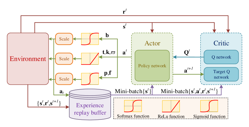
Figure 3: A2C Architecture

Algorithm 1 A2C-EI

Require: Initialize policy parameters $\theta$, Q-function parameter $\phi$.

Initialize target network weights $\phi_{\mathrm{targ}}$.

Initialize experience replay buffer $\mho$.

Initialize the total number of time steps for the RL training phase $T_{\mathrm{step}}$.

Repeat

while $t\leq T_{\mathrm{step}}$ do

     Observer state $\mathbf{s}^{t}$ and select action $\mathbf{a}^{t}\sim\pi_{\theta}(\cdot|\mathbf{s}^{t})$.

     Apply ECS and ACS then scale $\mathbf{a}^{t}$.

     Execute $\mathbf{a}^{t}$ in the environment.

     Observer next state $\mathbf{s}^{t+1}$, reward $\mathbf{r}^{t}$ and the done flag $d$ whether $\mathbf{s}^{t+1}$ is terminal.

     Store $\left(\mathbf{s}^{t},\mathbf{a}^{t},\mathbf{r}^{t},\mathbf{s}^{t+1},d\right)$ in experience replay buffer $\mho$.

     If $\mathbf{s}^{t+1}$ is terminal, reset the environment state.

     for $i$ in range (however many updates) do

         Randomly sample a batch of transitions

         $\mathcal{B}=\{\left(\mathbf{s}^{t},\mathbf{a}^{t},\mathbf{r}^{t},\mathbf{s}^{t+1},d\right)\}\in\mho$

         Compute targets for the Q-functions:

$$y \left(\mathbf{r}^{t},\mathbf{s}^{t+1},d\right)=\mathbf{r}^{t}+\gamma(1-d)\left(\min Q_{\phi_{\mathrm{targ}}}\left(\mathbf{s}^{t+1},\tilde{\mathbf{a}}^{t+1}\right)\right.$$

$$\left.\quad-\alpha\log\pi_{\theta}(\tilde{\mathbf{a}}^{t+1}|\mathbf{s}^{t+1})\right),\quad\tilde{\mathbf{a}}^{t+1}\in\pi^{t+1}\left(\cdot\mid\mathbf{s}^{t}\right),$$

where $\tilde{\mathbf{a}}^{t+1}$ is highlighted that the next actions have to be sampled fresh from the policy, whereas by contrast, $\mathbf{s}^{t+1}$ and $\mathbf{r}^{t}$ come from the experience relay buffer $\mho$.

         Update Q-functions by one step of gradient descent using

$$\nabla_{\phi}\frac{1}{|\mathcal{B}|}\sum\left(Q_{\phi_{\mathrm{targ}}}\left(\mathbf{s}^{t},\mathbf{a}^{t}\right)-y\left(\mathbf{r}^{t},\mathbf{s}^{t+1},d\right)\right)^{2}.$$

         Update policy by one step of gradient ascent using

$$\nabla_{\theta}\frac{1}{|\mathcal{B}|}\sum_{\mathbf{s}^{t}\in\mathcal{B}}\left(\min Q_{\phi}\left(\mathbf{s}^{t},\tilde{\mathbf{a}}^{t}_{\theta}(\mathbf{s}^{t})\right)-\alpha\log\pi_{\theta}(\tilde{\mathbf{a}}^{t}_{\theta}(\mathbf{s}^{t})|\mathbf{s}^{t})\right)^{2}.$$

         Update target networks with

$$\phi_{\mathrm{targ}}\leftarrow\rho\phi_{\mathrm{targ}}+(1-\rho)\phi,$$

where $\rho$ is polyak.      

until convergence

V Simulation Evaluation

In this section, we study the performance of the proposed SCFL for IoT networks with RTS by using computer simulation results. All statistical results are averaged over $10$ independent runs.

V-A IoT Network Setting

The BS is located at the center of a circular area with a radius of $1$ km, serving 100 users uniformly distributed. The path loss model is given by $128.1+37.6\log_{10}d$, where $d$ is the distance between the BS and the user (in km). The standard deviation of shadow fading is 8 dB, and the Gaussian noise power spectral density is $n_{0}=-174$ dBm/Hz. The transmit power is in the range of (0, 10] W, and the system bandwidth is $B=20$ MHz. We define the max number of sampling data skipped as $100$, and CPU frequency on each user is $f_{u}=5$ GHz. The number of CPU cycles for computing one sample data $C_{u}$ is uniformly distributed in [1:3] $\times 10^{4}$ cycles/sample, and computation capacity is in the normalized range (0,2] GHz. The effective switched capacitance in local computation is $\kappa=10^{-28}$. To evaluate the FL transmission, we use the ResNet-9 with a data size of $28$ MB.

V-B AI Model settings

To properly simulate the AI task behavior, we must consider the key features that capture all characteristics of training data and training AI model, i.e., $L$-smooth and $\mu$-strongly convex. To this end, we deploy a classification task on Convolutional Neural Network (CNN) on the CIFAR-10 dataset [29]. We sample data and feed through the AI model to consider the Hessian of the loss function. We follow the theory [30, 31, 32] that the minimizer tends to be the sharpest at the initial phase of the AI training. Therefore, by considering the Hessian of the loss function of the untrained AI model with the specific dataset, we can have the minimizer with the highest $2$nd derivative value, which is approximately close to the $L$-smooth and $\mu$ strongly convex value. Our theoretical implementation for $L$-smooth and $\mu$ strongly convex estimation can be found via experimental evaluation code. According to our evaluation, we found that the $L$ and $\mu$ value on MNIST and CIFAR-10 dataset is higher than $90$ and $150$, respectively. Therefore, we choose the $L$ and $\mu$ for our experimental evaluation with a set of values with an absolute value equal to: $\{100,125,150,175,200\}$ ($L$ are the set with positive values while $\mu$ are the sets with negative one).

V-C Iteration Time Bound Evaluation

Fig. 4 describes the influence of the sampling rate on the bound of convergence rate to verify the correctness of our bounded function in (26). We evaluate the crucial parameters, including sampling delay, $L$-smooth, global accuracy, and the number of users.

Fig. 4a shows the convergence rate by varying the sampling period from $0.01$s to $0.1$s. At the delay level with $\tau_{u}=0.01$s, the number of global iterations rapidly decreases from over $1000$ to just over $100$ rounds at the converged point, reducing nearly tenfold as the number $k$ increases from $0$ to $100$. When $\tau_{u}$ reaches $0.0325$s or higher, the number of rounds needed for convergence decreases to 600 and stabilizes around $400$ at $k=0$. Afterward, the number of iterations quickly reaches convergence at approximately $100$ rounds when $k=40$. Therefore, striking a balance between the choice of $\tau_{u}$ and the number of skip samples $k$ aids the SCFL algorithm in achieving stable and rapid convergence.

Fig. 4b compares different levels of data complexity (i.e., $L$-smoothness coefficient); containing sharper minimizers and higher $L$-smooth values. We can observe that as the $L$-smoothness level increases, the number of iterations required for the SCFL algorithm to converge also increases. This indicates that optimizing an FL algorithm is dependent on the variations in dataset complexity. As such, for datasets with low complexity like MNIST or CIFAR-10, we only need a small number of iterations for the algorithm to reach convergence.

Fig. 4c illustrates the influence of the bound of convergence rate by the variations in global accuracy. We recall that the global accuracy $\varpi$ represents the difference between the training model parameters and the optimal model parameters, and a lower global accuracy indicates a better match. When the global accuracy is lower, the number of rounds required to achieve convergence increases as mathematically shown in (26). Therefore, it is essential to strike a balance between the number of rounds for convergence and the global accuracy $\varpi$ to ensure optimization. As observed, for $\varpi$ values within the range of $[0.06,0.2]$, only around 200 iterations are needed for the SCFL algorithm to converge with approximately $k=20$.

Fig. 4d represents the influence of the number of users on the number of iterations required for the SCFL algorithm to converge. As $U$ increases, the complexity of the system model increases, leading to a higher number of iterations needed for convergence. When the number of users is sufficiently large (i.e., $U=100$), the number of iterations for SCFL to converge exceeds 6000 rounds. For $U$ values smaller than 100, the algorithm can quickly reach convergence with $k=20$, and the required number of rounds also decreases by 10 times compared to scenarios with a large number of users in the network. Notably, regardless of the network size, we can control the sampling rate to speed up the learning process of SCFL.

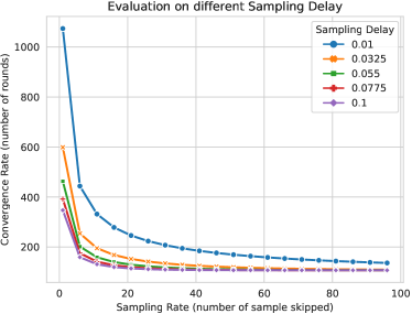
(a)

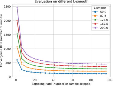
(b)

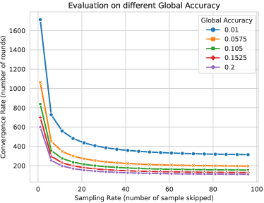
(c)

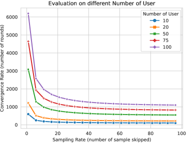
(d)

Figure 4: Illustration of the lower boundary on the number of global iterations (a) with different learning rates, and (b) with the different number of user values. (c) with different sampling delays, and (d) with different $L$-smooth values.

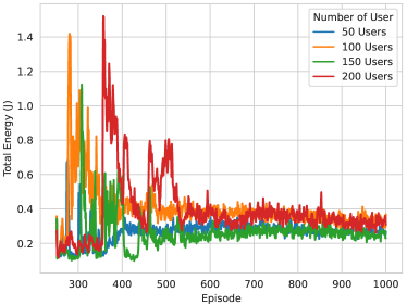
(a)

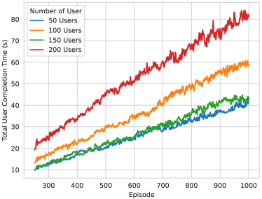
(b)

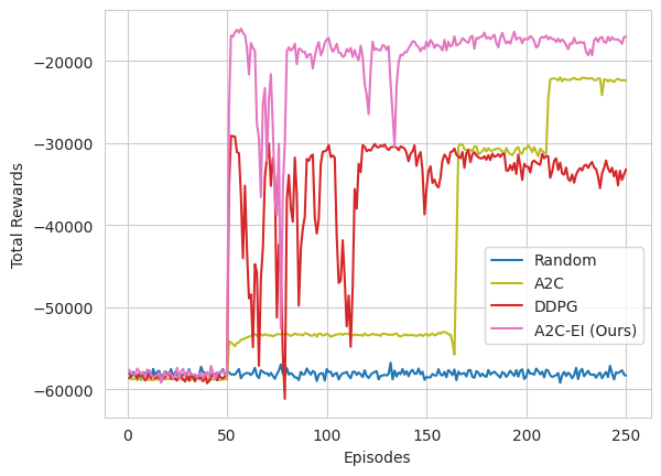
(c)

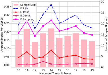
(d)

Figure 5: Illustration of DRL performance for SCFL. (a) Average energy per user in a different number of users scenario, (b) Completion time versus maximum transmit power, (c) Comparison between proposed A2C-EI with other baselines (d) Total energy versus maximum transmit power.

V-D Learning Performance of SCFL

Figures 5a and 5b illustrate the changes in total energy consumption and total completion time during the training process with different numbers of users. As described in Fig. 4d, as $U$ increases, the FL model becomes more complex, resulting in a higher number of global rounds. In Fig. 5a, during the first 500 episodes, the highest energy consumption occurs with $U=200$, and the lowest with $U=50$, respectively. However, after 500 episodes, the total energy converges, and there is little difference among different user counts.

As the number of episodes increases, the total completion time linearly increases in Fig. 5b. The total completion time is separated for different user numbers. Specifically, with $U=200$, the total completion time is the highest, and with $U=50$, it is the lowest. The linear change in total completion time is caused by the number of samples skipped in (1), which plays a crucial role in the problem. To reduce energy consumption, the model must decrease the number of samples skipped at the initialization time to approximately half of the largest number of skipped samplings. Consequently, the number of global iterations must increase, leading to a linear increase in total energy consumption.

V-E Performance Comparison

Fig. 5c illustrates the convergence performance of the A2C-EI algorithm that we propose in comparison to two other baselines, i.e., A2C [33] and DDPG [34]. Based on our observations and the reward definition presented in Section IV-B, the total reward increases and reaches convergence when it achieves a relatively stable value in all three methods: A2C-EI, A2C, and DDPG, except for the random scheme. Moreover, we have noticed that A2C-EI outperforms both A2C and DDPG regarding the total reward, while A2C performs better than DDPG. The higher performance of A2C comes at the cost of configuring all cases in problem (28) as mentioned in Section IV-C, leading to the need for multiple learning iterations to achieve the highest reward. On the other hand, our A2C-EI algorithm integrates A2C with resource constraints for output actions, thus resulting in a more optimized efficiency compared to the regular A2C algorithm.

Fig. 5d illustrates the influence of the maximum transmit power on the average energy consumption of each user. The graph consists of four curves representing the total energy consumption, transmission energy, computation energy, and sampling energy. The total energy consumption for each user is depicted by the distribution of energy types used for transmission, computation, and sampling. We observe that the optimal energy level lies at the maximum transmit power of $\{10,12,19\}$ W, and users consume higher energy at maximum power levels $\{11,14\}$ W. This fluctuation is attributed to the impact of the agent’s choice of the number of samples skipped for each maximum transmit power it learns. Hence, it is evident that the appropriate selection of the maximum transmit power and the number of samples skipped is crucial in improving energy efficiency.

VI Conclusion

In this paper, we have introduced a novel FL framework called SCFL and carried out the mathematical proof of the convergence analysis on the test set with arbitrary aspects. Our focus is on analyzing the data sampling characteristics in RTS distributed systems. By considering the impact of sampling delay between consecutive data samples on AI learning efficiency, our proposed SCFL ensures energy efficiency in the FL system while maintaining high performance on the test dataset. Notably, our research contributes significantly by being the first to propose a convergence analysis on the test dataset. This pioneering work lays a strong foundation for future research in optimizing FL networks. Specifically, it opens avenues to explore the relationship between data-related features, such as the number of training data and data relevance among distributed devices, and the FL convergence via the generalization gap.

Appendix A Inductive generalization gap

Based on Lagrange theory [35]:

$$f^{\prime}(c)=\frac{f(a)-f(b)}{b-a},$$ (45)

where $f(a)=\nabla\mathcal{L}_{u}\left(\omega^{(n)}+\vartheta_{u}^{(n)}\right)$,$f(b)=\nabla\mathcal{L}_{u}\left(\omega^{(n)}\right)$, $f(c)=\nabla\mathcal{L}_{u}\left(\omega\right)$. As a result

$$\left(\nabla\mathcal{L}_{u}\left(\omega^{(n)}+\vartheta_{u}^{(n)}\right)-\nabla\mathcal{L}_{u}\left(\omega^{(n)}\right)\right)=\nabla^{2}\mathcal{L}_{u}(\omega)\vartheta_{u}^{(n)}$$ (46)

Considering the inequality on the left of Lemma 5 in [16], the formula (46) and the assumption 3 we have

$$\frac{1}{L} \left\|\nabla\mathcal{L}_{u}\left(\omega^{(n)}+\vartheta_{u}^{(n)}\right)-\nabla\mathcal{L}_{u}\left(\omega^{(n)}\right)\right\|^{2}$$

$$=\frac{1}{L}(\nabla\mathcal{L}_{u}\left(\omega^{(n)}+\vartheta_{u}^{(n)}\right)-\nabla\mathcal{L}_{u}\left(\omega^{(n)}\right))^{\mathrm{T}}$$

$$\times(\nabla\mathcal{L}_{u}\left(\omega^{(n)}+\vartheta_{u}^{(n)}\right)-\nabla\mathcal{L}_{u}\left(\omega^{(n)}\right))$$

$$=\frac{1}{L}(\nabla\mathcal{L}_{u}\left(\omega^{(n)}+\vartheta_{u}^{(n)}\right)-\nabla\mathcal{L}_{u}\left(\omega^{(n)}\right))^{\mathrm{T}}\nabla^{2}\mathcal{L}_{u}(\omega)\vartheta_{u}^{(n)}$$

$$\leq\frac{1}{L}(\nabla\mathcal{L}_{u}\left(\omega^{(n)}+\vartheta_{u}^{(n)}\right)-\nabla\mathcal{L}_{u}\left(\omega^{(n)}\right))^{\mathrm{T}}L\boldsymbol{I}\vartheta_{u}^{(n)}$$

$$=\left(\nabla\mathcal{L}_{u}\left(\omega^{(n)}+\vartheta_{u}^{(n)}\right)-\nabla\mathcal{L}_{u}\left(\omega^{(n)}\right)\right)^{\mathrm{T}}\vartheta_{u}^{(n)}.$$ (47)

Similarly for the inequality on the right of Lemma 5 in [16] provided that assumption 4 obtains the formula

$$\frac{1}{L} \left\|\nabla\mathcal{L}_{u}\left(\omega^{(n)}+\vartheta_{u}^{(n)}\right)-\nabla\mathcal{L}_{u}\left(\omega^{(n)}\right)\right\|^{2}$$

$$\leq\left(\nabla\mathcal{L}_{u}\left(\omega^{(n)}+\vartheta_{u}^{(n)}\right)-\nabla\mathcal{L}_{u}\left(\omega^{(n)}\right)\right)^{\mathrm{T}}\vartheta_{u}^{(n)}$$

$$\leq\frac{1}{\mu}\left\|\nabla\mathcal{L}_{u}\left(\omega^{(n)}+\vartheta_{u}^{(n)}\right)-\nabla\mathcal{L}_{u}\left(\omega^{(n)}\right)\right\|^{2}.$$ (48)

For the optimal solution $\omega^{*}$ of $\mathcal{L}\left(\omega^{*}\right)$, we always have $\nabla\mathcal{L}\left(\omega^{*}\right)=\mathbf{0}$. Combining (10) and (A), we also have $\mu{I}\preceq$ $\nabla^{2}\mathcal{L}(\omega)$, which indicates that

$$\left\|\nabla\mathcal{L}(\omega)-\nabla\mathcal{L}\left(\omega^{*}\right)\right\|\geq\mu\left\|\omega-\omega^{*}\right\|$$ (49)

and

$$\mathcal{L}(\omega^{*})\geq\mathcal{L}(\omega)+\nabla\mathcal{L}(\omega)^{\mathrm{T}}\left(\omega^{*}-\omega\right)+\frac{\mu}{2}\left\|\omega^{*}-\omega\right\|^{2}.$$ (50)

As a result, we have

$$\|\nabla\mathcal{L}(\omega)\|^{2} =\left\|\nabla\mathcal{L}(\omega)-\nabla\mathcal{L}\left(\omega^{*}\right)\right\|^{2}$$

$$\stackrel{{\scriptstyle\leavevmode\nobreak\ \eqref{E:B4}}}{{\geq}}\mu\left\|\nabla\mathcal{L}(\omega)-\nabla\mathcal{L}\left(\omega^{*}\right)\right\|\left\|\omega-\omega^{*}\right\|$$

$$\geq\mu\left(\nabla\mathcal{L}(\omega)-\nabla\mathcal{L}\left(\omega^{*}\right)\right)^{\mathrm{T}}\left(\omega-\omega^{*}\right)$$

$$=\mu\nabla\mathcal{L}(\omega)^{\mathrm{T}}\left(\omega-\omega^{*}\right)$$

$$\stackrel{{\scriptstyle\leavevmode\nobreak\ \eqref{E:B5}}}{{\geq}}\mu\left(\mathcal{L}(\omega)-\mathcal{L}\left(\omega^{*}\right)\right)$$ (51)

which proves (52):

$$\|\nabla\mathcal{L}(\omega)\|^{2}\geq\mu\nabla\mathcal{L}(\omega)^{\mathrm{T}}\left(\omega-\omega^{*}\right).$$ (52)

For the optimal solution of the problem (II-B), the first-order derivative condition always holds, i.e.,

$$\nabla\mathcal{L}_{u}\left(\omega^{(n)}+\vartheta_{u}^{(n)*}\right)-\nabla\mathcal{L}_{u}\left(\omega^{(n)}\right)+\xi\nabla\mathcal{L}\left(\omega^{(n)}\right)=\mathbf{0}$$ (53)

$$\Rightarrow\nabla\mathcal{L}_{u}\left(\omega^{(n)}+\vartheta_{u}^{(n)*}\right)=\nabla\mathcal{L}_{u}\left(\omega^{(n)}\right)-\xi\nabla\mathcal{L}\left(\omega^{(n)}\right).$$ (54)

With Taylor expansion [36] we have the formula:

$$f(x_{t}+\Delta x)\approx f(x_{t})+(\Delta x)^{\mathrm{T}}\nabla f(x_{t})+\frac{1}{2}(\Delta x)^{\mathrm{T}}\nabla^{2}f(x_{t})\Delta x$$ (55)

We are now ready to prove Theorem 1 with the above inequalities and equalities, we have

$$\widetilde{\mathcal{L}}\left(\omega^{(n+1)}\right)=\mathcal{L}\left(\omega^{(n+1)}\right)+\mathfrak{R}_{\textrm{glob}}^{(n+1)}$$

$$\stackrel{{\scriptstyle\leavevmode\nobreak\ \eqref{Eq:10}}}{{=}}\mathcal{L}\left(\omega^{(n)}+\frac{1}{U}\sum^{U}_{u=1}\vartheta_{u}^{(n)}\right)+\mathfrak{R}_{\textrm{glob}}^{(n+1)}$$

$$\stackrel{{\scriptstyle\leavevmode\nobreak\ \eqref{Eq:Taylor},\mathrm{Assumption}\leavevmode\nobreak\ \ref{eq:YangA1}}}{{\leq}}\mathcal{L}\left(\omega^{(n)}\right)+\frac{1}{U}\sum_{u=1}^{U}\nabla\mathcal{L}\left(\omega^{(n)}\right)^{\mathrm{T}}\vartheta_{u}^{(n)}+\mathfrak{R}_{\textrm{glob}}^{(n+1)}$$

$$\quad+\frac{L}{2U^{2}}\left\|\sum_{u=1}^{U}\vartheta_{u}^{(n)}\right\|^{2}$$

$$\stackrel{{\scriptstyle\leavevmode\nobreak\ \eqref{Eq:10}}}{{=}}\mathcal{L}\left(\omega^{(n)}\right)+\mathfrak{R}_{\textrm{glob}}^{(n+1)}+\frac{1}{U\xi}\sum_{u=1}^{U}\left[\mathcal{G}_{u}\left(\omega^{(n)},\vartheta_{u}^{(n)}\right)\right.$$

$$\left.\quad+\nabla\mathcal{L}_{u}\left(\omega^{(n)}\right)\vartheta_{u}^{(n)}-\mathcal{L}_{u}\left(\omega^{(n)}+\vartheta_{u}^{(n)}\right)\right]$$

$$\quad+\frac{L}{2U^{2}}\left\|\sum_{u=1}^{U}\vartheta_{u}^{(n)}\right\|^{2}$$

$$\stackrel{{\scriptstyle\leavevmode\nobreak\ \eqref{Eq:Taylor},\mathrm{Assumption}\leavevmode\nobreak\ \ref{eq:YangA2}}}{{\leq}}\mathcal{L}\left(\omega^{(n)}\right)+\mathfrak{R}_{\textrm{glob}}^{(n+1)}$$

$$\quad+\frac{1}{U\xi}\sum_{u=1}^{U}\left[\mathcal{G}_{u}\left(\omega^{(n)},\vartheta_{u}^{(n)}\right)-\mathcal{L}_{u}\left(\omega^{(n)}\right)-\frac{\mu}{2}\left\|\vartheta_{u}^{(n)}\right\|^{2}\right]$$

$$\quad+\frac{L}{2U^{2}}\left\|\sum_{u=1}^{U}\vartheta_{u}^{(n)}\right\|^{2}.$$ (56)

To analyze Equation (A), base on (14), we replace $\omega^{(n+1)}$ with $\omega^{(n)}+\frac{1}{U}\sum^{U}_{u=1}\vartheta_{u}^{(n)}$. In the next, with the Taylor expansion in (55), we decompose

$$\mathcal{L}\left(\omega^{(n)}+\frac{1}{U}\sum^{U}_{u=1}\vartheta_{u}^{(n)}\right)=\mathcal{L}\left(\omega^{(n)}\right)$$

$$+\frac{1}{U}\sum_{u=1}^{U}\nabla\mathcal{L}\left(\omega^{(n)}\right)^{\mathrm{T}}\vartheta_{u}^{(n)}+\frac{\nabla^{2}\mathcal{L}(w)}{2U^{2}}\left\|\sum_{u=1}^{U}\vartheta_{u}^{(n)}\right\|^{2}$$

then combine with assumption 3, we have the inequality $\nabla^{2}F(\omega^{(n)})\leq LI$, we replace $\nabla^{2}F(\omega^{(n)})$ with $L$. Based on (14) replace

$$\nabla\mathcal{L}\left(\omega^{(n)}\right)^{\mathrm{T}}\vartheta_{u}^{(n)}=\frac{1}{\xi}\left[\mathcal{G}_{u}\left(\omega^{(n)},\vartheta_{u}^{(n)}\right)\right.$$

$$\left.\quad+\nabla\mathcal{L}_{u}\left(\omega^{(n)}\right)\vartheta_{u}^{(n)}-\mathcal{L}_{u}\left(\omega^{(n)}+\vartheta_{u}^{(n)}\right)\right]$$

In the next step, using Taylor expansion to decompose $\mathcal{L}_{u}\left(\omega^{(n)}+\vartheta_{u}^{(n)}\right)$, based on the assumption 3
$\nabla\mathcal{L}_{u}\left(\omega^{(n)}\right)\vartheta_{u}^{(n)}-\mathcal{L}_{u}\left(\omega^{(n)}+\vartheta_{u}^{(n)}\right)$ then is replaced by $-\mathcal{L}_{u}\left(\omega^{(n)}\right)-\frac{\mu}{2}\left\|\vartheta_{u}^{(n)}\right\|^{2}$.

According to (72), we have

$$\mathfrak{R}_{\textrm{glob}}^{(n)}=\frac{1}{U}\sum_{u=1}^{U}\mathfrak{R}_{u}^{(n)}$$

$$\mathfrak{R}_{\textrm{glob}}^{(n+1)}=\frac{1}{U}\sum_{u=1}^{U}\mathfrak{R}_{u}^{(n+1)}.$$

In addition, applying Lemmas 3, and 4, we have the followings

$$\mathfrak{R}_{u}^{(n+1)}-\mathfrak{R}_{u}^{(n)}$$

$$\leq\|\vartheta_{u}^{(n)}\|^{2}2^{H(\mathrm{Z})}\sqrt{2\left[H\left(p\left(z|\mathrm{Z}\right)\right)-I\left(p\left(z|\tilde{\mathrm{Z}}\right),p\left(z|\mathrm{Z}\right)\right)\right]}$$

$$+\frac{1}{2}\|\vartheta_{u}^{(n)}\|^{2}L2^{H(\mathrm{Z})}\sqrt{2\left[H\left(p\left(z|\mathrm{Z}\right)\right)-I\left(p\left(z|\tilde{\mathrm{Z}}\right),p\left(z|\mathrm{Z}\right)\right)\right]}$$

$$=\left(L+2\right)2^{H(\mathrm{Z})-1}\sqrt{2\left[H\left(p\left(z|\mathrm{Z}\right)\right)-I\left(p\left(z|\tilde{\mathrm{Z}}\right),p\left(z|\mathrm{Z}\right)\right)\right]}$$

$$\quad\times\|\vartheta_{u}^{(n)}\|^{2}$$

$$=\frac{\left(L+2\right)\Psi}{2}\|\vartheta_{u}^{(n)}\|^{2},$$ (57)

where $\Psi$ is the generalization gap statement and is demonstrated as:

$$\Psi=2^{H(\mathrm{Z})}\sqrt{2\left[H\left(p\left(z|\mathrm{Z}\right)\right)-I\left(p\left(z|\tilde{\mathrm{Z}}\right),p\left(z|\mathrm{Z}\right)\right)\right]}.$$ (58)

Thus, component $\mathfrak{R}_{\textrm{glob}}^{(n+1)}$ in (A) can be replaced by $\frac{1}{U}\sum_{u=1}^{U}\mathfrak{R}_{u}^{(n+1)}$. In addition, based on (A), component $\frac{1}{U}\sum_{u=1}^{U}\mathfrak{R}_{u}^{(n+1)}$ can be decomposed into the following:

$$\frac{1}{U}\sum_{u=1}^{U}\mathfrak{R}_{u}^{(n+1)}=\frac{1}{U}\sum_{u=1}^{U}\mathfrak{R}_{u}^{(n)}+\frac{1}{U}\sum_{u=1}^{U}\frac{\left(L+2\right)\Psi}{2}\|\vartheta_{u}^{(n)}\|^{2}.$$

From there, Equation (A) becomes

$$\widetilde{\mathcal{L}}\left(\omega^{(n+1)}\right)$$

$$\leq\mathcal{L}\left(\omega^{(n)}\right)+\frac{1}{U}\sum_{u=1}^{U}\mathfrak{R}_{u}^{(n+1)}$$

$$\quad+\frac{1}{U\xi}\sum_{u=1}^{U}\left[\mathcal{G}_{u}\left(\omega^{(n)},\vartheta_{u}^{(n)}\right)-\mathcal{L}_{u}\left(\omega^{(n)}\right)-\frac{\mu}{2}\left\|\vartheta_{u}^{(n)}\right\|^{2}\right]$$

$$\quad+\frac{L}{2U^{2}}\left\|\sum_{u=1}^{U}\vartheta_{u}^{(n)}\right\|^{2}$$

$$\stackrel{{\scriptstyle\leavevmode\nobreak\ \eqref{Eq:Pr-Gap}}}{{\leq}}\mathcal{L}\left(\omega^{(n)}\right)+\frac{1}{U}\sum_{u=1}^{U}\mathfrak{R}_{u}^{(n)}+\frac{1}{U}\sum_{u=1}^{U}\frac{\left(L+2\right)\Psi}{2}\|\vartheta_{u}^{(n)}\|^{2}$$

$$\quad+\frac{1}{U\xi}\sum_{u=1}^{U}\left[\mathcal{G}_{u}\left(\omega^{(n)},\vartheta_{u}^{(n)}\right)-\mathcal{L}_{u}\left(\omega^{(n)}\right)-\frac{\mu}{2}\left\|\vartheta_{u}^{(n)}\right\|^{2}\right]$$

$$\quad+\frac{L}{2U^{2}}\left\|\sum_{u=1}^{U}\vartheta_{u}^{(n)}\right\|^{2}.$$ (59)

Based on

$$\mathcal{L}\left(\omega^{(n)}\right)+\frac{1}{U}\sum_{u=1}^{U}\mathfrak{R}_{u}^{(n)}=\mathcal{L}\left(\omega^{(n)}\right)+\mathfrak{R}^{(n)}_{\textrm{glob}}=\widetilde{\mathcal{L}}\left(\omega^{(n)}\right)$$

and according to the triangle inequality and mean inequality that

$$\left\|\frac{1}{U}\sum_{u=1}^{U}\vartheta_{u}^{(n)}\right\|^{2}\leq\left(\frac{1}{U}\sum_{u=1}^{U}\left\|\vartheta_{u}^{(n)}\right\|\right)^{2}\leq\frac{1}{U}\sum_{u=1}^{U}\left\|\vartheta_{u}^{(n)}\right\|^{2},$$ (60)

we use $\widetilde{\mathcal{L}}\left(\omega^{(n)}\right)$ in place of $\mathcal{L}\left(\omega^{(n)}\right)+\frac{1}{U}\sum_{u=1}^{U}\mathfrak{R}_{u}^{(n)}$. Besides, based on (60), $\frac{L}{2U^{2}}\left\|\sum_{u=1}^{U}\vartheta_{u}^{(n)}\right\|^{2}$ could be replaced by $\frac{L}{2U^{2}}\sum_{u=1}^{U}\left\|\vartheta_{u}^{(n)}\right\|^{2}$. Combining the commutative, associative, and distributive properties in mathematics, Equation (A) can be transformed as follows

$$\widetilde{\mathcal{L}}\left(\omega^{(n+1)}\right)$$

$$\stackrel{{\scriptstyle\leavevmode\nobreak\ \eqref{E:B9}}}{{\leq}}\widetilde{\mathcal{L}}\left(\omega^{(n)}\right)+\frac{1}{U}\sum_{u=1}^{U}\frac{\left(L+2\right)\Psi}{2}\|\vartheta_{u}^{(n)}\|^{2}$$

$$\quad+\frac{1}{U\xi}\sum_{u=1}^{U}\left[\mathcal{G}_{u}\left(\omega^{(n)},\vartheta_{u}^{(n)}\right)-\mathcal{L}_{u}\left(\omega^{(n)}\right)-\frac{\mu}{2}\left\|\vartheta_{u}^{(n)}\right\|^{2}\right]$$

$$\quad+\frac{L}{2U^{2}}\sum_{u=1}^{U}\left\|\vartheta_{u}^{(n)}\right\|^{2}$$

$$=\widetilde{\mathcal{L}}\left(\omega^{(n)}\right)+\left[\frac{\left(L+2\right)\Psi}{2}+\frac{L}{2U}\right]\frac{1}{U}\sum_{u=1}^{U}\|\vartheta_{u}^{(n)}\|^{2}$$

$$\quad+\frac{1}{U\xi}\sum_{u=1}^{U}\left[\mathcal{G}_{u}\left(\omega^{(n)},\vartheta_{u}^{(n)}\right)-\mathcal{L}_{u}\left(\omega^{(n)}\right)-\frac{\mu}{2}\left\|\vartheta_{u}^{(n)}\right\|^{2}\right]$$

$$=\widetilde{\mathcal{L}}\left(\omega^{(n)}\right)+\frac{1}{U\xi}\sum_{u=1}^{U}\left[\mathcal{G}_{u}\left(\omega^{(n)},\vartheta_{u}^{(n)}\right)-\mathcal{L}_{u}\left(\omega^{(n)}\right)\right.$$

$$\left.\quad\frac{1}{2}\left(\xi\left(L+2\right)\Psi+\frac{\xi L}{U}-\mu\right)\left\|\vartheta_{u}^{(n)}\right\|^{2}\right].$$ (61)

Based on (12), we can obtain

$$\mathcal{G}_{u}\left(\omega^{(n)},\vartheta_{u}^{(n)}\right)-\mathcal{L}_{u}\left(\omega^{(n)}\right)$$

$$\stackrel{{\scriptstyle\leavevmode\nobreak\ \eqref{eq:Yang11}}}{{=}}\mathcal{G}_{u}\left(\omega^{(n)},\vartheta_{u}^{(n)}\right)-\mathcal{G}_{u}\left(\omega^{(n)},0\right)$$

$$=\mathcal{G}_{u}\left(\omega^{(n)},\vartheta_{u}^{(n)}\right)-\mathcal{G}_{u}\left(\omega^{(n)},\vartheta_{u}^{(n)*}\right)$$

$$\quad-\left[\mathcal{G}_{u}\left(\omega^{(n)},0\right)-\mathcal{G}_{u}\left(\omega^{(n)},\vartheta_{u}^{(n)*}\right)\right]$$

$$\stackrel{{\scriptstyle\leavevmode\nobreak\ \eqref{eq:Yang15}}}{{\leq}}(\varpi-1)\left[\mathcal{G}_{u}\left(\omega^{(n)},0\right)-\mathcal{G}_{u}\left(\omega^{(n)},\vartheta_{u}^{(n)*}\right)\right]$$

$$\stackrel{{\scriptstyle\leavevmode\nobreak\ \eqref{eq:Yang11}}}{{=}}(\varpi-1)\left[\mathcal{L}_{u}\left(\omega^{(n)}\right)-\mathcal{L}_{u}\left(\omega^{(n)}+\vartheta_{u}^{(n)*}\right)\right.$$

$$\left.\quad+\left(\nabla\mathcal{L}_{u}\left(\omega^{(n)}\right)-\xi\nabla\mathcal{L}\left(\omega^{(n)}\right)\right)^{\mathrm{T}}\vartheta_{u}^{(n)*}\right]$$

$$\stackrel{{\scriptstyle\leavevmode\nobreak\ \eqref{E:EB7}}}{{=}}(\varpi-1)\left[\mathcal{L}_{u}\left(\omega^{(n)}\right)-\mathcal{L}_{u}\left(\omega^{(n)}+\vartheta_{u}^{(n)*}\right)\right.$$

$$\left.\quad+\nabla\mathcal{L}_{u}\left(\omega^{(n)}+\vartheta_{u}^{(n)*}\right)^{\mathrm{T}}\vartheta_{u}^{(n)*}\right].$$ (62)

Based on assumption assumption 4, we can obtain

$$\mathcal{L}_{u}\left(\omega^{(n)}\right)\geq\mathcal{L}_{u}\left(\omega^{(n)}+\vartheta_{u}^{(n)*}\right)$$

$$\quad-\nabla\mathcal{L}_{u}\left(\omega^{(n)}+\vartheta_{u}^{(n)*}\right)^{\mathrm{T}}\vartheta_{u}^{(n)*}+\frac{\mu}{2}\left\|\vartheta_{u}^{(n)*}\right\|^{2}$$

$$\Leftrightarrow\mathcal{L}_{u}\left(\omega^{(n)}\right)-\mathcal{L}_{u}\left(\omega^{(n)}+\vartheta_{u}^{(n)*}\right)$$

$$\quad+\nabla\mathcal{L}_{u}\left(\omega^{(n)}+\vartheta_{u}^{(n)*}\right)^{\mathrm{T}}\vartheta_{u}^{(n)*}\geq\frac{\mu}{2}\left\|\vartheta_{u}^{(n)*}\right\|^{2}$$ (63)

Applying (A) to (A), we can obtain

$$\mathcal{G}_{u}\left(\omega^{(n)},\vartheta_{u}^{(n)}\right)-\mathcal{L}_{u}\left(\omega^{(n)}\right)\leq(1-\varpi)\frac{\mu}{2}\left\|\vartheta_{u}^{(n)*}\right\|^{2}.$$ (64)

Applying (64) to (A), we can receive

$$\widetilde{\mathcal{L}}\left(\omega^{(n+1)}\right)\leq\widetilde{\mathcal{L}}\left(\omega^{(n)}\right)+\frac{1}{U\xi}\sum_{u=1}^{U}\left[(1-\varpi)\frac{\mu}{2}\left\|\vartheta_{u}^{(n)*}\right\|^{2}\right.$$

$$\left.\quad+\frac{1}{2}\left(\xi\left(L+2\right)\Psi+\frac{\xi L}{U}-\mu\right)\left\|\vartheta_{u}^{(n)}\right\|^{2}\right].$$ (65)

From (A), the following relationship is received:

$$\left\|\vartheta_{u}^{(n)*}\right\|^{2}\geq\frac{1}{L^{2}}\|\nabla\mathcal{L}_{u}\left(\omega^{(n)}+\vartheta_{u}^{(n)*}\right)-\nabla\mathcal{L}_{u}\left(\omega^{(n)}\right)\|^{2}$$ (66)

In order to streamline the training process for local clients, we employ several techniques to enhance efficiency and performance. These include early stopping [37] for termination of training, small batch gradient descent [38] for improved optimization, and the utilization of dropout [39] to regularize the AI model. By implementing these strategies, we can achieve a more stable convergence of the local gradient training, resulting in reduced fluctuations and enhanced generalization. Consequently, the trained model satisfies the following condition:

$$\left\|\vartheta_{u}^{(n)}\right\|^{2}\leq\left\|\vartheta_{u}^{(n)*}\right\|^{2}.$$ (67)

Because of the lack of data changes caused by the environment, $\left\|\vartheta_{u}^{(n)*}\right\|^{2}$ cannot capture the entire observation of data, then $\nabla\mathcal{L}_{u}$ fluctuates more than $\nabla\widetilde{\mathcal{L}}_{u}$, and the inequality (66) becomes

$$\left\|\vartheta_{u}^{(n)*}\right\|^{2}\geq\frac{1}{L^{2}}\left\|\nabla\widetilde{\mathcal{L}}_{u}\left(\omega^{(n)}+\vartheta_{u}^{(n)*}\right)-\nabla\widetilde{\mathcal{L}}_{u}\left(\omega^{(n)}\right)\right\|^{2}$$ (68)

According to (67) and (A), we can obtain

$$\mathcal{L}\left(\omega^{(n+1)}\right)\leq\mathcal{L}\left(\omega^{(n)}\right)$$

$$\quad-\frac{\left(\xi\left(L+2\right)\Psi+\frac{\xi L}{U}-\varpi\mu\right)}{2U\xi}\sum_{u=1}^{U}\left\|\vartheta_{u}^{(n)*}\right\|^{2}$$

$$\leq\mathcal{L}\left(\omega^{(n)}\right)-\frac{\left(\xi\left(L+2\right)\Psi+\frac{\xi L}{U}-\varpi\mu\right)}{2UL^{2}\xi}\sum_{u=1}^{U}\left[\right.$$

$$\left.\times\left\|\nabla\mathcal{L}_{u}\left(\omega^{(n)}+\vartheta_{u}^{(n)*}\right)-\nabla\mathcal{L}_{u}\left(\omega^{(n)}\right)\right\|^{2}\right]$$

$$=\mathcal{L}\left(\omega^{(n)}\right)-\frac{\left(\xi\left(L+2\right)\Psi+\frac{\xi L}{U}-\varpi\mu\right)}{2UL^{2}\xi}\left\|\nabla\mathcal{L}\left(\omega^{(n)}\right)\right\|^{2}$$

$$\leq\mathcal{L}\left(\omega^{(n)}\right)-\frac{\left(\xi\left(L+2\right)\Psi+\frac{\xi L}{U}-\varpi\mu\right)}{2UL^{2}\xi}$$

$$\quad\times\left(\mathcal{L}\left(\omega^{(n)}\right)-\mathcal{L}\left(\omega^{*}\right)\right).$$ (69)

Based on (A), we obtain:

$$\mathcal{L}\left(\omega^{(n+1)}\right)-\mathcal{L}\left(\omega^{*}\right)$$

$$\leq\left(1-\frac{\left[\xi\left(L+2\right)\Psi+\frac{\xi L}{U}-\varpi\mu\right]}{2UL^{2}\xi}\right)\left(\mathcal{L}\left(\omega^{(n)}\right)-\mathcal{L}\left(\omega^{*}\right)\right)$$

$$\leq\left(1-\frac{\left[\xi\left(L+2\right)\Psi+\frac{\xi L}{U}-\varpi\mu\right]}{2UL^{2}\xi}\right)^{n+1}$$

$$\quad\times\left(\mathcal{L}\left(\omega^{(0)}\right)-\mathcal{L}\left(\omega^{*}\right)\right)$$

$$\leq\exp\left(-(n+1)\frac{\left[\xi\left(L+2\right)\Psi+\frac{\xi L}{U}-\varpi\mu\right]}{2UL^{2}\xi}\right)$$

$$\quad\times\left(\mathcal{L}\left(\omega^{(0)}\right)-\mathcal{L}\left(\omega^{*}\right)\right).$$ (70)

where the last inequality follows from the fact that $1-x\leq$ $\exp(-x)$. To ensure that $\mathcal{L}\left(\omega^{(n+1)}\right)-\mathcal{L}\left(\omega^{*}\right)\leq\varrho\left(\mathcal{L}\left(\omega^{(0)}\right)-\right.$ $\mathcal{L}\left(\omega^{*}\right)$ ), we have (26).

Appendix B Proof on lemma 2: Global generalization gap

We consider the global generalization gap as demonstrated in Equation (21):

$$\mathfrak{R}_{\textrm{glob}} =\mathbb{E}_{\{x_{i},y_{i}\}\sim\mathcal{D}}\left[\mathbb{E}_{(x,y)\sim\mathcal{D}^{\textrm{train}}}\left[\ell(x,y;w)\right]-\right.$$

$$\left.\leavevmode\nobreak\ \leavevmode\nobreak\ \leavevmode\nobreak\ \leavevmode\nobreak\ \leavevmode\nobreak\ \leavevmode\nobreak\ \leavevmode\nobreak\ \leavevmode\nobreak\ \leavevmode\nobreak\ \leavevmode\nobreak\ \leavevmode\nobreak\ \leavevmode\nobreak\ \leavevmode\nobreak\ \leavevmode\nobreak\ \leavevmode\nobreak\ \leavevmode\nobreak\ \leavevmode\nobreak\ \leavevmode\nobreak\ \mathbb{E}_{(x,y)\sim\mathcal{D}^{\textrm{test}}}\left[\ell(x,y;w)\right]\right]$$

$$=\mathbb{E}_{\{x_{i},y_{i}\}\sim\mathcal{D}}\left[\mathbb{E}_{u\in\mathcal{U}}\Big{\{}\mathbb{E}_{(x,y)\sim\mathcal{D}^{\textrm{train}}_{u}}\left[\ell(x,y;w)\right]\Big{\}}-\right.$$

$$\left.\leavevmode\nobreak\ \leavevmode\nobreak\ \leavevmode\nobreak\ \leavevmode\nobreak\ \leavevmode\nobreak\ \leavevmode\nobreak\ \leavevmode\nobreak\ \leavevmode\nobreak\ \leavevmode\nobreak\ \leavevmode\nobreak\ \leavevmode\nobreak\ \leavevmode\nobreak\ \leavevmode\nobreak\ \leavevmode\nobreak\ \leavevmode\nobreak\ \leavevmode\nobreak\ \leavevmode\nobreak\ \leavevmode\nobreak\ \mathbb{E}_{(x,y)\sim\mathcal{D}^{\textrm{test}}}\left[\ell(x,y;w)\right]\right]$$

$$=\mathbb{E}_{\{x_{i},y_{i}\}\sim\mathcal{D}}\left[\mathbb{E}_{u\in\mathcal{U}}\Big{\{}\mathbb{E}_{(x,y)\sim\mathcal{D}^{\textrm{train}}_{u}}\left[\ell(x,y;w)\right]\Big{\}}-\right.$$

$$\left.\leavevmode\nobreak\ \leavevmode\nobreak\ \leavevmode\nobreak\ \leavevmode\nobreak\ \leavevmode\nobreak\ \leavevmode\nobreak\ \leavevmode\nobreak\ \leavevmode\nobreak\ \leavevmode\nobreak\ \leavevmode\nobreak\ \leavevmode\nobreak\ \leavevmode\nobreak\ \leavevmode\nobreak\ \leavevmode\nobreak\ \leavevmode\nobreak\ \leavevmode\nobreak\ \leavevmode\nobreak\ \leavevmode\nobreak\ \mathbb{E}_{u\in\mathcal{U}}\mathbb{E}_{(x,y)\sim\mathcal{D}^{\textrm{test}}}\left[\ell(x,y;w)\right]\right]$$

$$=\mathbb{E}_{u\in\mathcal{U}}\Big{\{}\mathbb{E}_{\{x_{i},y_{i}\}\sim\mathcal{D}}\left[\mathbb{E}_{(x,y)\sim\mathcal{D}^{\textrm{train}}_{u}}\left[\ell(x,y;w)\right]-\right.$$

$$\left.\leavevmode\nobreak\ \leavevmode\nobreak\ \leavevmode\nobreak\ \leavevmode\nobreak\ \leavevmode\nobreak\ \leavevmode\nobreak\ \leavevmode\nobreak\ \leavevmode\nobreak\ \leavevmode\nobreak\ \leavevmode\nobreak\ \leavevmode\nobreak\ \leavevmode\nobreak\ \leavevmode\nobreak\ \leavevmode\nobreak\ \leavevmode\nobreak\ \leavevmode\nobreak\ \leavevmode\nobreak\ \leavevmode\nobreak\ \mathbb{E}_{(x,y)\sim\mathcal{D}^{\textrm{test}}}\left[\ell(x,y;w)\right]\right]\Big{\}}.$$ (71)

Thus, we can have the equivalent equality:

$$\mathfrak{R}_{\textrm{glob}}=\mathbb{E}_{u\in\mathcal{U}}[\mathfrak{R}_{u}]\leq\sum^{U}_{u=1}\sqrt{\frac{2\sigma^{2}}{n_{u}}}c_{0}e^{-c_{1}(\tau_{u})}$$ (72)

Appendix C Proof on lemma 3: Unbiased Gradient and Bounded Variance

We decompose the gradients as follows:

$$\nabla\tilde{\mathcal{L}}\left(\omega^{(n)}\right)-\nabla\mathcal{L}\left(\omega^{(n)}\right)$$

$$=\Big{\lVert}\sum_{z\in\mathrm{Z}}\nabla\ell(z,w)\left[p\left(z|\tilde{\mathrm{Z}}\right)-p\left(z|\mathrm{Z}\right)\right]\Big{\rVert}$$

$$\overset{(a1)}{\leq}\lVert\nabla\ell(z,w)\rVert\Big{\lVert}p\left(z|\tilde{\mathrm{Z}}\right)-p\left(z|\mathrm{Z}\right)\Big{\rVert}$$

$$\overset{(a2)}{\leq}\|\vartheta_{u}^{(n)}\|\frac{1}{p\left(z|\mathrm{Z}\right)}\sqrt{2\mathrm{D_{KL}}\left[p\left(z|\tilde{\mathrm{Z}}\right)\|p\left(z|\mathrm{Z}\right)\right]},$$ (73)

where $(a1)$ is due to the Hölder’s inequality, and $(a2)$ is inferred based on the Pinsker Inequality [40]. Because $\tilde{\mathrm{Z}}$ is the empirical global dataset, we take $p\left(z|\tilde{\mathrm{Z}}\right)=1$ so we have

$$p\left(z|\mathrm{Z}\right)=\frac{p\left(z|\tilde{\mathrm{Z}}\right)p\left(\tilde{z}\right)}{p(z)}=\frac{1}{p(z)}=2^{H(\mathrm{Z})}$$ (74)

with $H(.)$ is the entropy of the dataset.

Based on the information theory we have the following:

$$\mathrm{D_{KL}}\left[p\left(z|\tilde{\mathrm{Z}}\right)\|p\left(z|\mathrm{Z}\right)\right]$$

$$=H\left(p\left(z|\tilde{\mathrm{Z}}\right),p\left(z|\mathrm{Z}\right)\right)-H\left(p\left(z|\tilde{\mathrm{Z}}\right)\right)$$

$$=\left[H\left(p\left(z|\tilde{\mathrm{Z}}\right),p\left(z|\mathrm{Z}\right)\right)-H\left(p\left(z|\tilde{\mathrm{Z}}\right)\right)-H\left(p\left(z|\mathrm{Z}\right)\right)\right]$$

$$\quad+H\left(p\left(z|\mathrm{Z}\right)\right)$$

$$=H\left(p\left(z|\mathrm{Z}\right)\right)$$

$$\quad-\left[H\left(p\left(z|\tilde{\mathrm{Z}}\right)\right)+H\left(p\left(z|\mathrm{Z}\right)\right)-H\left(p\left(z|\tilde{\mathrm{Z}}\right),p\left(z|\mathrm{Z}\right)\right)\right]$$

$$=H\left(p\left(z|\mathrm{Z}\right)\right)-I\left(p\left(z|\tilde{\mathrm{Z}}\right),p\left(z|\mathrm{Z}\right)\right).$$ (75)

Arcording to the (C), (74), (C) we have

$$\nabla\tilde{\mathcal{L}}\left(\omega^{(n)}\right)-\nabla\mathcal{L}\left(\omega^{(n)}\right)$$

$$\leq\|\vartheta_{u}^{(n)}\|2^{H(\mathrm{Z})}\sqrt{2\left[H\left(p\left(z|\mathrm{Z}\right)\right)-I\left(p\left(z|\tilde{\mathrm{Z}}\right),p\left(z|\mathrm{Z}\right)\right)\right]}$$ (76)

Appendix D Proof on lemma 4: Unbiased Hessian and Bounded Variance

We decompose the Hessians as follows:

$$\nabla^{2}\tilde{\mathcal{L}}\left(\omega^{(n)}\right)-\nabla^{2}\mathcal{L}\left(\omega^{(n)}\right)$$

$$=\Big{\lVert}\sum_{z\in\mathrm{Z}}\nabla^{2}\ell(z,w)\left[p\left(z|\tilde{\mathrm{Z}}\right)-p\left(z|\mathrm{Z}\right)\right]\Big{\rVert}$$

$$\overset{(b1)}{\leq}\lVert\nabla^{2}\ell(z,w)\rVert\Big{\lVert}p\left(z|\tilde{\mathrm{Z}}\right)-p\left(z|\mathrm{Z}\right)\Big{\rVert}$$

$$\overset{(b2)}{\leq}L\frac{1}{p\left(z|\mathrm{Z}\right)}\sqrt{2\mathrm{D_{KL}}\left[p\left(z|\tilde{\mathrm{Z}}\right)\|p\left(z|\mathrm{Z}\right)\right]},$$ (77)

where $(b1)$ is due to the Hölder’s inequality, and $(b2)$ is inferred based on the Pinsker Inequality [40], and the hessian follows the $L$-smooth assumption. Because $\tilde{\mathrm{Z}}$ is the empirical global dataset, we take $p\left(z|\tilde{\mathrm{Z}}\right)=1$ so we have:

$$p\left(z|\mathrm{Z}\right)=\frac{p\left(z|\tilde{\mathrm{Z}}\right)p\left(\tilde{z}\right)}{p(z)}=\frac{1}{p(z)}=2^{H(\mathrm{Z})}$$ (78)

with $H(.)$ is the entropy of the dataset. According to (C), (D) and (78) we have

$$\nabla^{2}\tilde{\mathcal{L}}\left(\omega^{(n)}\right)-\nabla^{2}\mathcal{L}\left(\omega^{(n)}\right)$$

$$\leq L2^{H(\mathrm{Z})}\sqrt{2\left[H\left(p\left(z|\mathrm{Z}\right)\right)-I\left(p\left(z|\tilde{\mathrm{Z}}\right),p\left(z|\mathrm{Z}\right)\right)\right]}$$ (79)

References

• [1] B. McMahan, E. Moore, D. Ramage, S. Hampson, and B. A. y. Arcas, “Communication-efficient learning of deep networks from decentralized data,” in Proc. Int. Conf. on Artificial Intelligence and Statistics.   PMLR, Apr. 2017, pp. 1273–1282.
• [2] W. Y. B. Lim, N. C. Luong, D. T. Hoang, Y. Jiao, Y.-C. Liang, Q. Yang, D. Niyato, and C. Miao, “Federated learning in mobile edge networks: A comprehensive survey,” IEEE Communications Surveys & Tutorials, pp. 2031–2063, Apr. 2020.
• [3] H. H. Yang, Z. Liu, T. Q. Quek, and H. V. Poor, “Scheduling policies for federated learning in wireless networks,” IEEE Trans. on Comm., pp. 317–333, Sep. 2019.
• [4] S. Wang, T. Tuor, T. Salonidis, K. K. Leung, C. Makaya, T. He, and K. Chan, “Adaptive federated learning in resource constrained edge computing systems,” IEEE Journ. on Sel. Areas in Comm. (JSAC), pp. 1205–1221, Mar. 2019.
• [5] T.-A. Nguyen, J. He, L. T. Le, W. Bao, and N. H. Tran, “Federated pca on grassmann manifold for anomaly detection in IoT networks,” in Proc. IEEE Conf. on Computer Comm. (INFOCOM), Jun. 2023, pp. 1387–1395.
• [6] M. Chen, O. Semiari, W. Saad, X. Liu, and C. Yin, “Federated echo state learning for minimizing breaks in presence in wireless virtual reality networks,” IEEE Trans. on Wire. Comm., pp. 177–191, 2019.
• [7] S. Samarakoon, M. Bennis, W. Saad, and M. Debbah, “Distributed federated learning for ultra-reliable low-latency vehicular communications,” IEEE Trans. on Comm., pp. 1146–1159, Nov. 2019.
• [8] S. P. Karimireddy, S. Kale, M. Mohri, S. Reddi, S. Stich, and A. T. Suresh, “SCAFFOLD: Stochastic controlled averaging for federated learning,” in Proceedings of the 37th International Conference on Machine Learning, Jul. 2020.
• [9] J. Konečnỳ, H. B. McMahan, D. Ramage, and P. Richtárik, “Federated optimization: Distributed machine learning for on-device intelligence,” arXiv preprint arXiv:1610.02527, Oct. 2016. [Online]. Available: https://arxiv.org/abs/1610.02527
• [10] S. Wang, T. Tuor, T. Salonidis, K. K. Leung, C. Makaya, T. He, and K. Chan, “When edge meets learning: Adaptive control for resource-constrained distributed machine learning,” in Proc. IEEE Conf. on Computer Comm. (INFOCOM), Apr. 2018, pp. 63–71.
• [11] K. Bonawitz, H. Eichner, W. Grieskamp, D. Huba, A. Ingerman, V. Ivanov, C. Kiddon, J. Konečnỳ, S. Mazzocchi, B. McMahan et al., “Towards federated learning at scale: System design,” Proc. of Mach. Learn. and Syst., pp. 374–388, Mar. 2019. [Online]. Available: https://arxiv.org/abs/1902.01046
• [12] M.-D. Nguyen, S.-M. Lee, Q.-V. Pham, D. T. Hoang, D. N. Nguyen, and W.-J. Hwang, “Hcfl: A high compression approach for communication-efficient federated learning in very large scale iot networks,” IEEE Trans. on Mob. Comp., pp. 1–13, Jul. 2022.
• [13] M.-D. Nguyen, Q.-V. Pham, D. T. Hoang, L. Tran-Thanh, D. N. Nguyen, and W.-J. Hwang, “Label driven knowledge distillation for federated learning with non-IID data,” arXiv preprint arXiv:2209.14520, Mar. 2022.
• [14] M. Chen, Z. Yang, W. Saad, C. Yin, H. V. Poor, and S. Cui, “A joint learning and communications framework for federated learning over wireless networks,” IEEE Trans. on Wire. Comm., pp. 269–283, Oct. 2020.
• [15] N. H. Tran, W. Bao, A. Zomaya, M. N. H. Nguyen, and C. S. Hong, “Federated learning over wireless networks: Optimization model design and analysis,” in IEEE INFOCOM 2019 - IEEE Conference on Computer Communications, Jun. 2019, pp. 1387–1395.
• [16] Z. Yang, M. Chen, W. Saad, C. S. Hong, and M. Shikh-Bahaei, “Energy efficient federated learning over wireless communication networks,” IEEE Trans. on Wire. Comm., vol. 20, no. 3, pp. 1935–1949, Nov. 2020.
• [17] C. T. Dinh, N. H. Tran, M. N. H. Nguyen, C. S. Hong, W. Bao, A. Y. Zomaya, and V. Gramoli, “Federated learning over wireless networks: Convergence analysis and resource allocation,” IEEE/ACM Transactions on Networking, vol. 29, no. 1, pp. 398–409, Nov. 2020.
• [18] S. Barua, M. M. Islam, X. Yao, and K. Murase, “MWMOTE–majority weighted minority oversampling technique for imbalanced data set learning,” IEEE Trans. on Knowl. and Data Eng., Feb. 2014.
• [19] D. Russo and J. Zou, “How much does your data exploration overfit? controlling bias via information usage,” IEEE Transactions on Information Theory, vol. 66, no. 1, pp. 302–323, Oct. 2020.
• [20] T. Li, A. K. Sahu, M. Zaheer, M. Sanjabi, A. Talwalkar, and V. Smith, “Federated optimization in heterogeneous networks,” arXiv:1812.06127, Apr. 2020. [Online]. Available: https://arxiv.org/abs/1812.06127
• [21] G. Neu, G. K. Dziugaite, M. Haghifam, and D. M. Roy, “Information-theoretic generalization bounds for stochastic gradient descent,” in Proceedings of Machine Learning Research, vol. 134.   PMLR, Aug. 2021, pp. 3526–3545.
• [22] A. Xu and M. Raginsky, “Information-theoretic analysis of generalization capability of learning algorithms,” in Proceedings of the 31st International Conference on Neural Information Processing Systems, Dec. 2017.
• [23] Y. Cao and Q. Gu, “Generalization bounds of stochastic gradient descent for wide and deep neural networks,” in 33rd Conference on Neural Information Processing Systems, Dec. 2019.
• [24] A. Fallah, A. Mokhtari, and A. Ozdaglar, “Personalized federated learning with theoretical guarantees: A model-agnostic meta-learning approach,” in Proc. Adv. Neural Inf. Process. Syst. (NeurIPS), Dec. 2020, pp. 3557–3568.
• [25] M. Min, L. Xiao, Y. Chen, P. Cheng, D. Wu, and W. Zhuang, “Learning-based computation offloading for IoT devices with energy harvesting,” IEEE Trans. on Vehi. Tech., pp. 1930–1941, Jan. 2019.
• [26] X. Chen, H. Zhang, C. Wu, S. Mao, Y. Ji, and M. Bennis, “Optimized computation offloading performance in virtual edge computing systems via deep reinforcement learning,” IEEE Internet of Things Journal, pp. 4005–4018, Oct. 2018.
• [27] J. Chen, S. Chen, Q. Wang, B. Cao, G. Feng, and J. Hu, “iRAF: A deep reinforcement learning approach for collaborative mobile edge computing IoT networks,” IEEE Internet of Things Journal, pp. 7011–7024, Apr. 2019.
• [28] S. P. Boyd and L. Vandenberghe, Convex Optimization.   Cambridge University Press, 2004.
• [29] A. Krizhevsky, “Learning multiple layers of features from tiny images,” University of Toronto, Tech. Rep., Aug. 2009.
• [30] L. Dinh, R. Pascanu, S. Bengio, and Y. Bengio, “Sharp minima can generalize for deep nets,” in Proc. Int. Conf. Mach. Learn. (ICML), July 2017.
• [31] P. Goyal, P. Dollár, R. Girshick, P. Noordhuis, L. Wesolowski, A. Kyrola, A. Tulloch, Y. Jia, and K. He, “Accurate, large minibatch sgd: Training imagenet in 1 hour,” arXiv, 2018.
• [32] Y. You, J. Li, S. Reddi, J. Hseu, S. Kumar, S. Bhojanapalli, X. Song, J. Demmel, K. Keutzer, and C.-J. Hsieh, “Large batch optimization for deep learning: Training bert in 76 minutes,” in Proc. Int. Conf. Rep. Learn. (ICLR), May 2020.
• [33] T. Haarnoja, A. Zhou, P. Abbeel, and S. Levine, “Soft actor-critic: Off-policy maximum entropy deep reinforcement learning with a stochastic actor,” in Proc. Int. Conf. Mach. Learn. (ICML), vol. 80, May 2018, pp. 1861–1870.
• [34] Z. Ding, R. Schober, and H. V. Poor, “No-pain no-gain: DL assisted optimization in energy-constrained cr-noma networks,” IEEE Trans. on Comm., pp. 5917–5932, 2021.
• [35] L. Hörmander, The Analysis of Linear Partial Differential Operators I: Distribution Theory and Fourier Analysis.   Springer, Mar. 2015.
• [36] P. Benigno and M. Woodford, “Linear-quadratic approximation of optimal policy problems,” Journal of Economic Theory, vol. 147, no. 1, pp. 1–42, Jan. 2012.
• [37] L. Prechelt, “Early stopping-but when?” in Neural Networks: Tricks of the Trade.   Springer, 1996, pp. 55–69.
• [38] B. E. Woodworth, K. K. Patel, and N. Srebro, “Minibatch vs local sgd for heterogeneous distributed learning,” in Proc. Adv. Neural Inf. Process. Syst. (NeurIPS), Mar. 2022, pp. 6281–6292.
• [39] P. Baldi and P. J. Sadowski, “Understanding dropout,” in Proc. Adv. Neural Inf. Process. Syst. (NeurIPS).   Curran Associates, Inc., Jan. 2013.
• [40] I. Csiszár and J. Körner, Information Theory: Coding Theorems for Discrete Memoryless Systems, 2nd ed.   Cambridge University Press, Aug. 2012.