Boosting Black-box Attack to Deep Neural Networks with Conditional Diffusion Models

Abstract

Existing black-box attacks have demonstrated promising potential in creating adversarial examples (AE) to deceive deep learning models. Most of these attacks need to handle a vast optimization space and require a large number of queries, hence exhibiting limited practical impacts in real-world scenarios. In this paper, we propose a novel black-box attack strategy, Conditional Diffusion Model Attack (CDMA), to improve the query efficiency of generating AEs under query-limited situations. The key insight of CDMA is to formulate the task of AE synthesis as a distribution transformation problem, i.e., benign examples and their corresponding AEs can be regarded as coming from two distinctive distributions and can transform from each other with a particular converter. Unlike the conventional query-and-optimization approach, we generate eligible AEs with direct conditional transform using the aforementioned data converter, which can significantly reduce the number of queries needed. CDMA adopts the conditional Denoising Diffusion Probabilistic Model as the converter, which can learn the transformation from clean samples to AEs, and ensure the smooth development of perturbed noise resistant to various defense strategies. We demonstrate the effectiveness and efficiency of CDMA by comparing it with nine state-of-the-art black-box attacks across three benchmark datasets. On average, CDMA can reduce the query count to a handful of times; in most cases, the query count is only ONE. We also show that CDMA can obtain $>99\%$ attack success rate for untarget attacks over all datasets and targeted attack over CIFAR-10 with the noise budget of $\epsilon=16$.

I Introduction

In recent years, Deep Learning (DL) has experienced rapid development, and DL models are widely deployed in many real-world applications, such as facial recognition [1], autonomous driving [2], financial services [3], etc. However, existing DL models have been proven to be fragile that they can be easily fooled by adding elaborately calculated imperceptible perturbations to the benign inputs, known as adversarial examples (AEs). Therefore, the security of DL models has been attracting more and more attention from researchers.

Typically, adversarial attacks can be classified into two categories based on their settings. The first one is white-box attacks [4, 5], where the attacker has complete information of the victim models, including the model structure, weights, gradients, etc. Such information can assist the attacker to achieve a very high attack success rate. A variety of attack techniques have been proposed to effectively generate AEs under the white-box setting, e.g., FGSM [6], C&W [4], etc.

The second one is black-box attacks [7, 8, 9, 10, 11], which is more practical in the real world. The attacker is not aware of the victim model’s information. He has to repeatedly query the victim model with carefully crafted inputs and adjust the perturbations based on the returned soft labels (prediction probability) or even hard labels [12, 13]. Many query-efficient and transfer-based attack methods have been proposed recently. However, they suffer from several limitations. First, these methods still need hundreds to thousands of queries to generate one AE [8]), especially in the targeted attack setting. This makes the attack costly in terms of computation resources, time and monetary expense, restricting their practicality in real-world scenarios. Besides, more queries can remarkably increase the risk of being detected [14]. Second, AEs generated by the noise-adding manner are easy to be identified or denoised, decreasing the attack performance to a large extent [15, 16]. Once the victim model is equipped with some defense mechanisms, the attacker needs to consume more model queries to optimize a new AE. Third, the quality of the generated AE highly depends on the similarity between the local surrogate model and the victim model, which normally cannot be guaranteed. This also limits the performance of existing attack methods.

Driven by the above drawbacks, the goal of this paper is to design new hard-label black-box attack approaches, which can generate AEs with limited queries for both untarget and targeted settings. This is challenging due to the restrictions of limited information about the victim model, and query budget. Our observation is that clean samples and their corresponding AEs follow two adjacent distributions, connected by certain relationships. This presents an opportunity to build a converter, which can easily transfer each clean sample to its corresponding AE without complex optimization operations. Following this hypothesis, we propose CDMA, a novel Conditional Diffusion Model Attack to attack black-box DL models efficiently. Different from prior attacks using the iterative query-and-optimization strategy, CDMA converts the AE generation task into an image translation task, and adopts a conditional diffusion model (i.e., the converter) to directly synthesize high-quality AEs. In detail, we first execute the diffusion process to train a conditional diffusion model with pre-collected pair-wised clean-adversarial samples, where the AEs are generated with white-box attack methods from local shadow models. During the training, the clean images are used as the condition to guide the diffusion model to generate eligible AEs from a given unique input. Once the diffusion model is trained, we can execute the reverse process for the clean input to formulate corresponding AEs.

Compared to existing works, CDMA has the following advantages. (1) It significantly improves the attack effectiveness by conditional synthesis instead of query and optimization. (2) CDMA does not rely on the inherent attribute of the target model. It only requires the hard labels to verify whether the victim model has been attacked successfully. As a result, the pre-trained diffusion model has a high generalization ability to attack any DL models. (3) Once the diffusion model is well-trained, the attacker can batch-wisely sample sufficient candidate AEs, further improving the attack efficiency and scalability. (4) Benefiting from the smooth synthesizing processes, the formulated AEs are challenging to be purified and can keep high robustness against different defense mechanisms.

We evaluate CDMA on mainstream datasets (CIFAR-10, CIFAR-100 and Tiny-ImageNet-200), and compare it with state-of-the-art black-box attack methods, including pure black-box attacks (soft- and hard-label), query-based and transfer-based attacks. Extensive experiment results demonstrate our superior query efficiency. In all attack settings, CDMA achieves a comparable attack success rate to all baselines but with significantly reduced numbers of queries. Besides, AEs generated from CDMA exhibit higher robustness to several mainstream defense strategies. Finally, the empirical results of data-independent and model-independent attacks have validated our assumption, i.e., the clean and adversarial examples come from two disparate distributions, which can be transformed into each other, and the proposed CDMA can well learn this transformation relationship.

To summarize, our main contributions are as follows:

• We model the adversarial example generation as a distribution transform problem with a perfect data converter on certain conditions to achieve efficient black-box attacks.

• We build the data converter with a diffusion model and propose a novel diffusion model-based black-box attack named CDMA, which can directly formulate the corresponding AE by conditional sampling on the original clean image without the complex iterative process of query and optimization.

• CDMA can generate AEs with high attack ability and robustness. These AEs can be well transferred to different victim models and datasets.

• We perform extensive experiments to demonstrate the superiority of CDMA over state-of-the-art black-box methods, in terms of query efficiency, attack robustness and effectiveness in both untargeted and targeted settings.

The remainder of this paper is organized as follows: we briefly review the existing literature on adversarial attacks in Sec. II. We define our distribution transformation-based attack and propose the diffusion model-based CDMA method in Sec. III. In Sec. IV, we perform extensive experiments to show that CDMA is more efficient and effective than other baseline attacks under untarget and targeted situations. It can also successfully keep the high attack performance against different defense strategies. Finally, we conclude this paper in Sec. V.

II Related Work

Adversarial attacks against deep learning models refer to the process of intentionally manipulating benign inputs to fool well-trained models. Based on the setting, existing attacks can be classified into two categories: in the white-box setting, the attacker knows every detail about the victim model, based on which he creates the corresponding AEs. In the black-box setting, the attacker does not have the knowledge of the victim model, and are only allowed to query the model for AE generation. In this paper, we focus on the black-box one, which is more practical but also more challenging.

There are three types of techniques to achieve black-box adversarial attacks. The first one is transfer-based attacks. Papernot et al. [17] proposed the pioneering work towards black-box attacks, which first utilizes Jacobian-based Dataset Augmentation to train a substitute model by iteratively querying the oracle model, and then attacking the oracle using the transferability of AEs generated from the substitute model. TREMBA [18] trains a perturbation generator and traverses over the low-dimensional latent space. ODS [19] optimizes in the logit space to diversify perturbations for the output space. GFCS [20] searches along the direction of surrogate gradients and falls back to ODS. CG-Attack [21] combines a well-trained c-glow model and CAM-ES to extend attacks. However, these transfer-based attacks heavily rely on the similarity between the substitute model and the oracle model.

The second type is score-based attacks. Ilyas et al. [13] proposed a bandit optimization-based algorithm to integrate priors, such as gradient priors, to reduce the query counts and improve the attack success rate. Chen et al. [22] proposed zeroth order optimization-based attacks (ZOO) to directly estimate the gradients of the target DNN for generating AEs. Although this attack achieves a comparable attack success rate, its coordinate-wise gradient estimation requires excessive evaluations of the target model and is hence not query-efficient. AdvFlow [8] combines a normalized flow model and NES to search the adversarial perturbations in the latent space to balance the query counts and distortion and accelerate the attack process.

The third type is decision-based attacks, which are specifically designed for the hard-label setting. Boundary attack [12] is the earliest one that starts from a large adversarial perturbation and then seeks to reduce the magnitude of perturbation while keeping it adversarial. Bayes_Attack [9] uses Bayesian optimization to find adversarial perturbations in the low-dimension subspace and maps it back to the original input space to obtain the final perturbation. NPAttack [11] considers the structure information of pixels in one image rather than individual pixels during the attack with the help of a pre-trained Neural Process model. Rays [7] introduces a Ray Searching Method to reformulate the continuous problem of finding the nearest decision boundary as a discrete problem that does not require any zero-order gradient estimation, which significantly improves the previous decision-based attacks. Triangle Attack (TA) [10] optimizes the perturbation in the low-frequency space by utilizing geometric information for effective dimensionality reduction.

The above query-and-optimization black-box attacks are inefficient and uneconomical because they require thousands of queries on the target model. In this situation, the time and computational consumption could be very considerable. On the other hand, the performance of transfer-based black-box attacks is often limited by the similarity between the surrogate model and the oracle model. Besides, these attacks cannot extend to the data-independent or model-independent scenario or keep robustness to different defense strategies, which fades the attack capability to a considerable extent.

Therefore, it is necessary to have a method that can efficiently generate AEs within limited queries, which are effective against different models and datasets. We propose to use the diffusion model to achieve this goal. The diffusion model is an advanced technique for image translation tasks. We can train such a model to convert clean images to AEs against the black-box victim model. Our attack, CDMA, does not require a large number of queries or detailed information regarding the victim model in the attacking process and the formulated AEs can be resistant to most defense strategies.

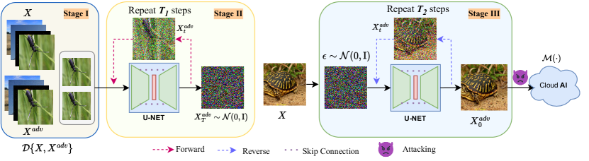
Figure 1: Overview of CDMA. $\mathcal{D}\{X,X^{adv}\}$ is the collected pair-wised clean and adversarial dataset and $X_{t}^{adv}$ is the adversarial example $X^{adv}$ at the forward or reverse step $t$. $\epsilon\sim\mathcal{N}(0,\mathrm{I})$ is the Gaussian noise and $\mathcal{M}(\cdot)$ is the target victim model.

III Methodology

III-A Problem Definition

Given a well-trained DNN model $\bm{\mathcal{M}}$ and an input $\bm{x}$ with its corresponding label $y$, we have $\bm{\mathcal{M}}(\bm{x})=y$. The AE $\bm{x}^{adv}$ is a neighbor of $\bm{x}$ that satisfies $\bm{\mathcal{M}}(\bm{x}^{adv})\neq y$ and $\left\|\bm{x}^{adv}-\bm{x}\right\|_{p}\leq\epsilon$, where $\bm{L}_{p}$ norm is used as the metric function and $\epsilon$ is a small noise budget. With this definition, the problem of generating an AE becomes a constrained optimization problem:

$$\bm{x}_{adv}=\underset{\left\|\bm{x}^{adv}-\bm{x}\right\|_{p}\leq\epsilon}{\mathop{arg\ max}\mathcal{L}}(\bm{\mathcal{M}}(\bm{x}^{adv})\neq y),$$ (1)

where $\mathcal{L}$ stands for a loss function that measures the confidence of the model outputs.

Existing attack methods normally utilize the information (e.g., the prediction results, model weights, etc.) obtained from the target model to optimize the above loss function. Different from them, in this paper, we convert the AE generation problem into an image-to-image task: an adversarial image $\bm{x}_{adv}$ can be regarded as a particular transformation from its corresponding clean image $\bm{x}$. These two different images ($\bm{x}$ and $\bm{x}_{adv}$) can be mutually transformed from each other by a converter. We choose a rising star generative model, the diffusion model, as our image converter and propose a Conditional Diffusion Model-based Attack framework for synthesizing AEs.

III-B Denoising Diffusion Probabilistic Models

Unlike VAE or Flow models, diffusion models are inspired by non-equilibrium thermodynamics to learn through a fixed process. The latent space has a relatively high dimensionality. It first defines a Markov chain of diffusion steps and corrupts the training data by continuously adding Gaussian noise until it becomes pure Gaussian noise. Then it reverses the process by removing noise and reconstructing the desired data. Once the model is well-trained, it can generate data through the learned denoising process by inputting randomly sampled noise. Here, we briefly review the representative Denoising Diffusion Probabilistic Models (DDPM) [23].

In the forward progress (i.e., adding noise), given an image $x_{0}\sim q(x)$, the diffusion process can obtain $x_{1},x_{2},...,x_{T}$ by adding Gaussian noise $T$ times, respectively. This process can be expressed as a Markov chain:

$$q(x_{t}|x_{t-1}) =\mathcal{N}(x_{t};\sqrt{1-\beta_{t}}x_{t-1},\beta_{t}\mathrm{I}),$$ (2)

$$q(x_{1:T}|x_{0}) =\prod_{t=1}^{T}q(x_{t}|x_{t-1})=\prod_{t=1}^{T}(x_{t};\sqrt{1-\beta_{t}}x_{t-1},\beta_{t}\mathrm{I})$$

where $t\in{1,2,...,T}$, $\left\{\beta_{t}\in(0,1)\right\}_{t=1}^{T}$ is the hyper-parameter of the Gaussian distribution’s variance. In this process, $x_{t}$ tends to be pure Gaussian noise with the increase of $t$. It finally becomes the Standard Gaussian noise $\mathcal{N}(0,\mathrm{I})$ when $T\to\infty$.

Suppose $\alpha_{t}:=1-\beta_{t}$ and $\bar{\alpha}_{t}:={\textstyle\prod_{i=1}^{T}\alpha_{i}}$. Then $x$ of arbitrary $t$ can be written in the following closed form:

$$q(x_{t}|x_{0})=\mathcal{N}(x_{t};\sqrt{\bar{a}_{t}}x_{0},(1-a_{t})\mathrm{I}),$$ (3)

$$x_{t}=\sqrt{\bar{\alpha}_{t}}x_{0}+\sqrt{1-\bar{\alpha}_{t}}\delta$$

where $\delta\sim\mathcal{N}(0,\mathrm{I})$. $x_{t}$ satisfies $q(x_{t}|x_{0})=\mathcal{N}(x_{t};\sqrt[]{\bar{a_{t}}}x_{0},(1-\bar{a_{t}})\mathrm{I})$.

The reverse process is the denoising of diffusion. If we can gradually obtain the reversed distribution $q(x_{t-1}|x_{t})$, we can restore the original image $x_{0}$ from the standard Gaussian distribution $\mathcal{N}(0,\mathrm{I})$.

As $q(x_{t}|x_{t-1})$ is a Gaussian distribution and $\beta_{t}$ is small enough, $q(x_{t-1}|x_{t})$ is a Gaussian distribution. However, we do not have a simple way to infer $q(x_{t-1}|x_{t})$. DDPM adopts a deep neural network, typically U-Net, to predict the mean and covariance of $x_{t-1}$ of the given input $x_{t}$. In this situation, the reverse process can be written as the parameterized Gaussian transitions:

$$p_{\theta}(X_{0:T)=P(x_{T}})\prod_{t=1}^{T}p_{\theta}(x_{t-1}|x_{t}),$$ (4)

$$P_{\theta}(x_{t-1}|x_{t})=\mathcal{N}(x_{t-1};\mu(x_{t},t),{\textstyle\sum_{\theta}(x_{t},t)})$$

With Bayes’s theorem, DDPM predicts the noise $\delta_{\theta}(x_{t},t)$ instead and computes $\mu(x_{t},t)$ as follows:

$$\mu(x_{t},t)=\frac{1}{\sqrt{\alpha_{t}}}(x_{t}-\frac{\beta_{t}}{\sqrt{1-\bar{\alpha}_{t}}}\delta_{\theta}(x_{t},t))$$ (5)

III-C Conditional Diffusion Model Attack (CDMA)

The whole framework of CDMA is illustrated in Figure 1, which can be split into the following three stages: training sample collection, model training (forward process), and AE generating (reverse process). Specifically, in Stage I, the attacker collects the clean-adversarial example pairs, where the adversarial examples are built from local shadow models using standard white-box attack techniques. In Stage II, the attacker trains a conditional diffusion model with the pair-wised $(\bm{x},\bm{x}_{adv})$ sampled from the pre-collocated dataset $\mathcal{D}\{X,X^{adv}\}$. The conditional diffusion model is composed of a series of encoder-decoder-like neural networks (UNET [24] is adopted in this work). Once the model is well-fitted, the attacker can perform the attacks against the victim model in a sampling manner in Stage III instead of a query-and-optimization way. Below we give details of each stage.

III-C1 Training Sample Collection

Recall that our training data are paired with clean and adversarial samples, where the clean example is used as an inference image and concatenated with its corresponding adversarial example to compose the diffusion model’s input. More specifically, for a given dataset, we first use typical white-box attack methods (e.g., PGD [25] and et al.) to attack the local shadow model and obtain the corresponding adversarial examples, which are then paired with the original clean examples to formulate the training dataset $\mathcal{D}=\{X,X^{adv}\}$ of our diffusion model.

III-C2 Conditional Diffusion Model Training

The core of training a diffusion model is to make it predict reliable noise $\delta$. Unlike [23], we need to consider the additional conditional variable $x$. We use $\delta$ to represent the real noise added to $x^{adv}$ at each step $t$, and use $\hat{\delta}_{\theta}$ to represent the noise predicted by model $f(\cdot)$ (U-NET in this paper). Then the final objective function can be written as:

$$\mathcal{L}=E_{t,\{x,x_{0}^{adv}\},\delta}\left\|\delta-\hat{\delta}_{\theta}(x_{t}^{adv},t,x)\right\|_{p}$$ (6)

where $t\sim[1,2,...,T],\{x,x_{0}^{adv}\}\sim\mathcal{D}\{x,x^{adv}\},x_{t}^{adv}\sim q(x_{t}^{adv}|x_{0}^{adv},x)$, $\delta\sim\mathcal{N}(0,\mathrm{I})$, $\|\cdot\|_{p}$ represents the $L_{p}$-norm and $p\in\{0,1,2,L_{\infty}\}$. As demonstrated in [26], $L_{1}$ yields significantly lower sample diversity compared to $L_{2}$. Since we aim to generate diversified adversarial examples, we also adopt $L_{2}$, i.e., MSE, as our loss function to constrain the true noise $\delta$ and the predicted noise $\hat{\delta}_{\theta}$.

Algorithm 1 Conditional Diffusion Model Training

0:  $\{x,x^{adv}\}$: the clean image and adversarial image pair; $t\sim\mathcal{U}({1,...,T})$: The time-steps belong to Uniform distribution.

0:  The well-trained model $M(\cdot)$.

1:  repeat

2:     Take the gradient step on $\mathcal{L}=E_{t,\{x,x_{0}^{adv}\},\delta}\left\|\delta-\hat{\delta}_{\theta}(x_{t}^{adv},t,x)\right\|_{p}$.

3:  until converged

Algorithm 2 Conditional Diffusion Model Attacking

0:  $\bm{\mathcal{C}}$: the target model to be attacked; $\bm{x}$: the clean image, the conditioning information for conditional sampling; $\bm{Q}$: the maximum querying number; $q$: the current querying number; $\epsilon$: the noise budget.

0:  The adversarial example $\bm{x}_{adv}$ used for attack.

1:  $\bm{x}_{T}^{adv}\sim\mathcal{N}(\bm{0},\bm{I})$.

2:  while $q<=Q$ do

3:     for $t=T,...,1$ do

4:        $\bm{z}\sim\mathcal{N}(\bm{0},\bm{I})$ if $t>1$, else $\bm{z}=0$

5:        $\bm{x_{t-1}}\sim q(x_{t-1}|x)$

6:        $\bm{x}_{t-1}^{adv}\leftarrow p_{\theta}(\bm{x}_{t-1}^{adv}|\bm{x}_{t}^{adv},\bm{x})$

7:     end for

8:     $\delta=clip(\bm{x}_{0}^{adv}-x,-\epsilon,\epsilon)$

9:     $\bm{x}^{adv}=clip(x+\delta,0,1)$

10:     if $\bm{x}^{adv}$ attack $\bm{\mathcal{C}}$ successfully then

11:        break.

12:     end if

13:  end while

14:  return $\bm{x}^{adv}$

III-C3 Generate Adversarial Examples.

In CDMA, the attacker generates adversarial examples for benign images by sampling from the well-trained conditional diffusion model. Our generation process becomes sampling from the conditional distribution $P(x_{0}^{adv}|c)$, where $c$ is the clean image $x$. As the aforementioned sampling process of DDPM [23, 27] (Eq. 4), the conditional sampling can be written as follows:

$$p_{\theta}(x_{0}^{adv}|x)=\int p_{\theta}(x_{0:T}^{adv}|x)dx_{1:T}^{adv}$$ (7)

$$p_{\theta}(x_{0}^{adv}|x)=p(x_{T}^{adv})\prod_{t=1}^{T}p_{\theta}(x_{t-1}^{adv}|x_{t}^{adv},x)$$

Here each transition $p_{\theta}(x_{t-1}^{adv}|x_{t}^{adv},x)$ in the sampling process depends on the condition $x$, i.e., the clean image. The sampling (Eq.4) in the conditional version is re-written as:

$$p_{\theta}(x_{t-1}^{adv}|x_{t}^{adv},x)=\mathcal{N}(x_{t-1}^{adv};\mu_{\theta}(x_{t}^{adv},t,x),{\textstyle\sum_{\theta}(x_{t}^{adv},t,x))}$$ (8)

As shown in Eq. 8, CDMA generates the adversarial example $\bm{x}^{adv}$ via the diffusion model’s reverse Markov process and starts from $\bm{x}_{0}^{adv}=\epsilon\sim\mathcal{N}(0,\mathrm{I})$ with the conditional clean image $x$. To make the final adversarial examples meet the similarity requirements, we impose the extra $clip(\cdot)$ constraints on $L_{\infty}$-norm as:

$$\bm{x}_{final}^{adv}=clip(clip(\bm{x}_{0}^{adv},x-\epsilon,x+\epsilon),0,1)$$ (9)

where $\epsilon$ is the adversarial perturbation budget.

The training and attacking algorithms of CDMA are listed in Alg. 1 and Alg. 2, respectively, which could help readers to re-implement our method step-by-step.

TABLE I: Experimental results on attack success rate and the query counts on CIFAR-10.

	Methods	VGG-19			Inception-V3			ResNet-50			DenseNet-169
		ASR	Avg.Q	Med.Q	ASR	Avg.Q	Med.Q	ASR	Avg.Q	Med.Q	ASR	Avg.Q	Med.Q
untarget	AdvFlow	80.60	396.79	358	61.5	423.68	358	63.20	403.76	358	65.87	440.29	409
	RayS	98.93	160.25	126	96.01	224.52	176.5	96.53	202.43	150	96.65	215.62	159
	Bayes_Attack	75.24	45.87	5	79.39	48.2	5	81.44	42.37	5	77.10	45.42	5
	TA	25.05	66.60	11	23.77	67.01	5	28.60	74.02	6	27.69	66.29	8
	NPAttack	97.75	225.79	150	96.73	229.3	150	96.11	234.72	150	96.54	239.45	150
	ODS	97.49	11.79	10	99.00	28.50	13	97.80	18.03	10	99.1	25.26	12
	GFCS	98.83	8.66	6	98.29	28.02	7	98.43	10.38	6	99.45	18.05	7
	CG-Attack	96.57	86.94	1	97.98	101.65	1	96.48	84.97	1	97.16	97.91	1
	MCG-Attack	96.87	75.41	1	98.14	80.67	1	97.38	76.92	1	99.10	81.67	1
	CDMA(Ours)	99.46	1.63	1	99.58	2.97	1	99.58	3.16	1	99.68	5.31	1
targeted	AdvFlow	10.93	653.12	600	9.16	674.17	650	10.64	672.13	650	9.87	681.67	650
	RayS	18.82	209.95	159	18.40	331.5	283	17.82	297.91	258	17.25	306.82	222
	Bayes_Attack	28.62	587.16	490	24.94	505.61	535	19.87	549.48	570	27.84	497.99	515
	TA	14.63	238.65	210	13.58	267.21	231	15.87	227.41	204	14.92	219.36	198
	NPAttack	48.71	279.16	250	51.87	278.13	200	47.40	400	450	42.88	322.92	300
	ODS	76.71	204.08	80	88.42	152.17	75	92.01	130.81	66	95.08	133.14	70
	GFCS	79.08	141.88	23	90.68	111.9	32	93.39	95.53	24.5	95.40	99.41	25
	CG-Attack	74.03	487.61	441	78.67	511.13	501	76.94	491.67	481	77.15	534.16	501
	MCG-Attack	79.17	361.47	281	81.92	306.28	261	80.69	297.63	261	78.16	342.19	301
	CDMA(Ours)	94.31	27.85	1	91.67	8.88	1	94.65	7.47	1	95.52	8.09	1

TABLE II: Experimental results on ASR and the query counts on CIFAR-100.

	Methods	VGG-19			Inception-V3			ResNet-50			DenseNet-169
		ASR	Avg.Q	Med.Q	ASR	Avg.Q	Med.Q	ASR	Avg.Q	Med.Q	ASR	Avg.Q	Med.Q
untarget	AdvFlow	75.30	321.02	256	79.00	392.24	358	76.10	365.17	307	81.80	354.82	307
	RayS	99.86	101.28	71	98.63	134.8	96	99.47	130.87	82	98.76	130.39	84.5
	Bayes_Attack	89.70	13.82	5	89.03	14.8	5	88.76	17.24	5	87.58	18.69	5
	TA	55.96	38.85	5	48.82	38.57	5	53.39	43.54	5	54.42	57.27	6
	NPAttack	94.74	161.34	100	94.11	172.84	100	95.39	173.39	100	94.61	174.54	100
	ODS	97.90	35.84	17	97.59	28.89	19	96.78	32.60	18	96.72	28.93	17
	GFCS	98.84	8.66	6	98.27	28.02	7	97.97	10.38	6	97.49	18.05	7
	CG–Attack	98.74	78.94	1	87.59	97.38	21	98.27	79.14	1	97.76	96.83	1
	MCG-Attack	98.87	69.19	1	90.64	84.61	1	98.82	71.66	1	98.47	85.73	1
	CDMA(Ours)	99.25	5.16	1	98.71	6.86	1	99.63	4.28	1	99.37	4.92	1
targeted	AdvFlow	7.12	697.58	650	8.32	681.65	650	7.98	657.29	600	8.42	642.13	600
	RayS	13.44	269.90	182	12.74	232.17	267	14.05	216.125	194	11.12	212.67	181
	Bayes_Attack	16.94	645.61	710	13.48	687.15	695	15.49	597.34	625	17.61	578.67	600
	TA	13.67	281.52	247	11.92	277.40	239	12.00	274.58	235	13.94	264.59	232
	NPAttack	40.59	451.63	400	41.25	318.52	300	42.13	487.35	450	40.38	507.49	550
	ODS	75.78	301.89	224.5	76.95	224.11	157	79.51	291.93	208	73.67	257.95	187
	GFCS	74.53	292.10	198	80.75	155.17	68.5	81.66	181.79	75	78.30	164.37	71
	CG-Attack	62.91	648.29	601	60.74	676.49	621	63.15	542.67	481	61.94	704.61	641
	MCG-Attack	66.28	546.58	481	62.18	516.94	441	67.16	486.27	441	63.35	536.93	501
	CDMA(Ours)	73.95	70.17	2	83.42	40.43	1	82.79	24.29	1	77.25	38.10	1

TABLE III: Experimental results on attack success rate and the query counts on Tiny-ImageNet.

	Methods	VGG-19			Inception-V3			ResNet-50			DenseNet-169
		ASR	Avg.Q	Med.Q	ASR	Avg.Q	Med.Q	ASR	Avg.Q	Med.Q	ASR	Avg.Q	Med.Q
untarget	AdvFlow	88.30	302.44	256	92.89	322.28	256	93.50	313.44	256	98.8	241.86	205
	RayS	98.98	100.2	68	99.39	117.83	68	98.77	107.73	67	99.64	93.5	65
	Bayes_Attack	74.13	24.14	5	76.28	66.13	5	72.41	24.83	5	80.00	26.37	5
	TA	69.32	73.62	18	64.72	82.41	18	67.76	71.74	16	78.29	59.53	11
	NPAttack	91.77	241.55	150	93.77	259.48	150	95.59	242.68	150	98.83	192.16	150
	ODS	99.61	43.47	24	99.17	45	30	99.53	42.28	27	98.82	47.43	25.5
	GFCS	98.41	36.64	9	99.37	35	11	99.21	36.38	10	99.67	25.12	8
	CG-Attack	98.34	97.81	21	97.73	113.94	21	97.62	136.81	21	98.16	127.43	21
	MCG-Attack	98.76	80.64	1	98.47	110.49	21	97.91	109.84	21	99.17	89.76	21
	CDMA(Ours)	99.67	3.90	1	99.55	7.27	1	99.71	5.53	1	99.83	3.75	1
targeted	AdvFlow	5.32	754.38	700	5.73	724.69	700	6.52	671.94	650	5.84	714.61	700
	RayS	9.27	255.57	215	8.89	223.17	197	10.45	192.33	223	9.72	217.70	184.5
	Bayes_Attack	10.94	284.64	245	13.14	297.92	305	12.49	273.25	280	11.76	318.16	315
	TA	8.64	263.59	243.5	7.48	316.78	284	8.12	323.43	251	8.47	297.69	267
	NPAttack	32.26	585.71	600	32.12	605.35	625	36.69	596.02	650	33.90	690.52	600
	ODS	74.09	391.22	271	81.01	336.33	286	81.80	340.50	280.5	80.64	341.62	252.5
	GFCS	79.37	298.25	235	81.54	220.46	110.5	84.83	250.64	142	82.34	326.30	157
	CG-Attack	71.67	367.45	381	69.46	416.97	401	73.97	437.41	421	68.63	443.37	421
	MCG-Attack	70.16	417.28	401	71.91	429.71	401	75.63	431.67	421	70.38	427.16	401
	CDMA(Ours)	77.95	46.04	1	82.20	26.87	1	85.13	17.80	1	82.82	23.40	1

IV Evaluation

We present the experimental results of CDMA. We first compare it with other black-box attack baselines in untarget and targeted scenarios. Then we measure the attack effectiveness against state-of-the-art defenses. Next, we show the results of data-independent and model-independent attacks. Finally, we show the ablation study results to explore the attack ability of CDMA under different settings.

IV-A Experimental Setup

Implementation. We set the maximum number of queries as $Q_{max}=1000$ to simulate a realistic attack scenario. We stop the attack once a specific input is mispredicted by the victim model successfully. We set the noise budget as $\epsilon=8/255.$ and $\epsilon=16/255.$, which is shortened as $\epsilon=8$ and $\epsilon=16$ for all attacks. To train the diffusion model in CDMA, the total number of diffusion steps is $T=2000$. The number of training epochs is $E=1e8$ with the batch size of $B=256$. The noise scheduler is ”linear” starting from $1e-6$ and ending with $0.01$. All the experiments are conducted on a GPU server with 4*NVIDIA Tesla A100 40GB GPU, 2*Xeon Glod 6112 CPU and RAM 512GB.

Datasets. We verify the performance of CDMA on three benchmark datasets for computer vision task, named CIFAR-10 [28], CIFAR-100 [28] and Tiny-ImageNet-200 [29]. In detail, CIFAR-10 contains 50,000 training images and 10,000 testing images with the size of $3\times 32\times 32$ from 10 classes; CIFAR-100 has 100 classes, including the same number of training and testing images as the CIFAR-10; Tiny-ImageNet-200 has 200 categories, containing about 1.3M samples for training and 50,000 samples for validation. In our experiments, we first generate adversarial examples using white-box attacks on the training set of the above three datasets to train the diffusion model, and then randomly sample 1,000 images from the test set of these datasets for attacks.

Models. We train a few widely-used deep neural networks, including VGG [30], Inception [31, 32], ResNet [33], and DenseNets [34] over the aforementioned datasets until the models achieve the best classification results. Among them, We adopt VGG-13, ResNet-18 and DeseNet-121 as the shadow models for all query- and transfer-based baselines and CDMA, while VGG-19, Inception-V3, ResNet-50 and DenseNet-169 as the victim models to be attacked for all the methods. The top-1 classification accuracy of these victim models are 90.48%, 84.51%, 94.07%, and 94.24% for CIFAR-10, 66.81%, 77.86%, 76.05% and 77.18% for CIFAR-100 and 57.62%, 65.89%, 65.41% and 56.04% for Tiny-ImageNet-200, respectively.

Baselines. We select nine state-of-the-art black-box attacks as the baselines, including score-based, decision-based, and query- and transfer-based methods. These include Rays [7], AdvFlow [8], Bayes_Attack [9], TA [10], NPAttack [11], ODS [19], GFCS [20], CG-Attack [21] and MCG-Attack [35]. We reproduce the attacks from the code released in the original papers with the default settings.

Metrics. We perform evaluations with the following metrics: Attack Success Rate (ASR) measures the attack effectiveness. Average and Median numbers of queries (Avg.Q and Med.Q) measure the attack efficiency.

IV-B Comparisons with Baseline Attacks

Tables I, II and III present the untarget and targeted attack performance comparison with all baselines under the noise budget $\epsilon=16$ on VGG-19, Inception-V3, ResNet-50, and DenseNet-169, respectively. Specifically, in both untarget and targeted situations, we observe that our proposed CDMA enjoys much higher efficiency in terms of the average and median numbers of queries, as well as much higher attack success rate than AdvFlow, Bayes_Attack and TA for all datasets. Compared to the rest baselines, although the attack success rate of CDMA does not exceed too much, in some cases, even lower than Rays (when extending the untarget attack on VGG-19 with CIFAR-100) and GFCS (when extending the targeted attack on VGG-19 with Tiny-ImageNet-200), the Avg.Q and Med.Q are always lowest than all methods, especially in the target setting. CDMA only needs several queries to obtain a near 100% attack success rate and the Med.Q of CDMA is 1. These experimental results demonstrate the superiority of our proposed method in terms of attack effectiveness and efficiency.

Table. IV presents the performance comparison of all attack baselines on VGG-19, Inception-V3, ResNet-50 and DenseNet-169, respectively, where the noise budget is set to $\epsilon=8$. Although the attack becomes more challenging with a small noise budget, compared with all the attack baselines, the proposed CDMA can also get the best attack performance in most situations. Especially the average and median queries of CDMA are still the lowest in all cases, which have exhibited the high effectiveness of the proposed methods.

TABLE IV: untarget attack on CIFAR-10, CIFAR-100 and Tiny-ImageNet, the noise budget is $\epsilon=8$.

	Methods	VGG-19			Inception-V3			ResNet-50			DenseNet-169
		ASR	Avg.Q	Med.Q	ASR	Avg.Q	Med.Q	ASR	Avg.Q	Med.Q	ASR	Avg.Q	Med.Q
CIFAR-10	AdvFlow	50.1	414.19	358	37.43	431.9	409	41.50	409.62	358	39.72	438.49	409
	RayS	80.96	303.45	231	75.08	342.30	286	79.06	339.32	254	77.14	331.54	255
	Bayes_Attack	33.73	91.57	8	36.80	95.01	5	38.92	84.93	7	34.98	78.45	6
	TA	7.56	95.39	14	5.60	63.24	5	6.37	52.58	7	7.16	87.95	9.5
	NPAttack	64.67	330.30	250	64.17	336.37	250	65.90	328.98	250	65.19	339.95	250
	ODS	95.16	11.71	9	92.10	25.19	12	96.24	15.84	10	95.80	26.28	12
	GFCS	94.7	25.49	6	91.30	37.83	7	96.20	22.27	6	94.80	29.03	7
	CG-Attack	94.84	125.95	1	92.94	137.64	41	94.87	115.57	1	94.91	134.63	1
	MCG-Attack	95.07	105.63	1	93.25	110.91	1	95.71	99.14	1	95.68	100.84	1
	CDMA(Ours)	94.36	9.38	1	94.08	16.66	1	96.66	10.83	1	96.50	10.78	1
CIFAR-100	AdvFlow	58.68	340.3	307	53.10	375.77	307	52.41	383.79	358	55.30	369.44	307
	RayS	94.54	197.51	135.5	86.93	227.89	158	92.00	214.4	139.5	91.19	222.94	148.5
	Bayes_Attack	65.16	36.62	5	65.21	46.50	5	63.86	45.34	5	62.61	56.06	5
	TA	22.43	63.26	5	17.45	58.55	5	22.60	66.49	5	21.35	64.26	5
	NPAttack	71.20	236.55	150	70.43	253.03	150	70.13	240.68	150	69.13	271.60	150
	ODS	93.90	33.13	11	94.65	18.89	12	92.70	22.00	12	91.70	28.27	14
	GFCS	94.20	33.44	5	95.50	30.65	6	93.60	30.42	6	92.00	29.41	6
	CG-Attack	93.67	112.67	21	93.47	138.59	21	93.29	100.93	41	92.61	125.48	41
	MCG-Attack	94.15	105.64	1	94.39	110.94	1	93.68	89.14	1	93.62	98.07	1
	CDMA(Ours)	92.42	16.17	1	90.70	19.28	1	94.75	18.17	1	92.07	20.20	1
Tiny-ImageNet	AdvFlow	76.98	319.2	256	79.96	334.42	256	82.3	319.08	256	95.70	273.27	205
	RayS	89.51	185.96	124.5	87.97	199.93	132	88.10	170.94	109	93.56	160.74	98
	Bayes_Attack	43.58	59.27	5	40.18	77.91	5	42.23	82.09	5	55.36	53.51	5
	TA	34.66	100.99	26	29.29	107.02	30.5	33.07	103.05	24.5	49.61	98.07	29
	NPAttack	71.57	315.75	250	73.32	315.14	250	74.46	317.67	250	88.70	57.39	150
	ODS	91.50	42.55	23	91.21	45.47	28	91.17	44.10	28	93.31	42.33	28
	GFCS	92.70	62.18	9	93.40	71.52	12	92.10	79.95	12	95.00	49.39	9
	CG-Attack	92.64	111.42	21	87.65	164.97	41	88.49	157.49	41	90.48	146.73	21
	MCG-Attack	92.93	104.91	21	89.46	146.18	41	89.07	139.73	21	91.86	124.61	21
	CDMA(Ours)	93.57	19.69	1	93.53	31.98	1	92.13	27.26	1	95.34	11.63	1

Figure 2 shows the attack success rate versus the number of queries for all baseline methods over CIFAR-10, CIFAR-100, and Tiny-ImageNet-200 in untarget and target attack settings. Again we can see that CDMA achieves the highest attack success rate in most situations and the best query efficiency compared with other black-box attack baselines. The results show that our proposed CDMA can achieve the highest attack success rate under the same query counts. Note that CDMA can obtain a boosting attack success rate at the first few queries, especially under targeted attack settings, while other attacks only can obtain a satisfactory attack success rate after hundreds of queries.

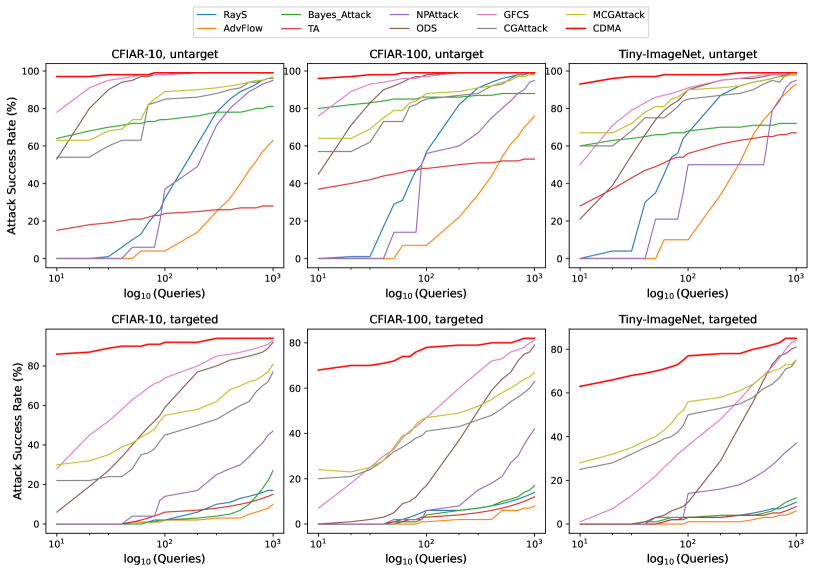
Figure 2: Queries vs. ASR on CIFAR-100 and Tiny-ImageNet for untarget and targeted attack settings. The maximal query counts are limited to 1000 and the noise budget’s $L_{\infty}$ norm is set to $\epsilon=16$.

IV-C Adversarial Robustness to Defense Strategies

To further evaluate the generated adversarial examples’ robustness, we adopt some defense methods to purify or pre-process the malicious examples, and then measure their effectiveness. The defense methods in our consideration involve JPEG compression (JPEG) [36], NRP [37], pixel deflection (PD) [38], GuidedDiffusionPur (GDP) [16], RP-Regularizer (RP) [39], BitDepthReduce (BDR) [40] and MedianSmoothing2D (MS) [40]. We first synthesize adversarial examples on ResNet-50 for CIFAR-10, and then measure their attack success rate against these defense strategies. The results are shown in Table. V. Among all the black-box attack methods, our proposed method has the highest attack success rate in most cases, which implies the adversarial examples generated by CDMA are more robust to current defense methods compared with other attacks.

IV-D Data-independent and Model-independent Attacks

IV-D1 Data-independent Attack

We carry out attacks across different datasets to verify the generalization of our CDMA. The datasets include STL-10 [41], Caltech-256 [42], Places-365 [43]) and CeleBA [44]. These datasets are not used for training the diffusion model, and we only sample images from their test set to test the effectiveness of CDMA.

TABLE V: The attack success rate under defense strategies.

Methods	JPEG	NRP	PD	GDP	RP	BDR	MS
AdvFlow	46.36	44.46	87.15	27.30	61.86	46.79	52.88
RayS	60.99	15.73	90.07	21.65	63.36	57.44	58.73
Bayes_Attack	43.36	22.01	87.89	25.52	66.02	80.99	49.35
TA	42.91	33.20	82.81	21.88	53.82	71.88	45.49
NPAttack	38.93	31.84	90.40	11.61	64.25	59.54	41.89
ODS	21.08	41.74	91.10	4.91	66.42	41.84	30.19
GFCS	21.72	42.34	89.79	6.36	66.73	44.35	29.23
CG-Attack	47.61	38.72	78.16	18.67	59.86	68.29	52.63
M-CG-Attack	48.43	40.81	82.69	22.38	60.53	69.62	54.27
DMA(Ours)	72.61	77.01	90.40	44.20	93.86	91.53	80.19

TABLE VI: The attack success rate of data-independent attack.

Noise	Models	STL-10		Places-365		Caltech256		CeleBA
		ASR	Avg.Q	ASR	Avg.Q	ASR	Avg.Q	ASR	Avg.Q
$\epsilon=8$	VGG-19	94.29	10.15	99.5	4.47	96.9	11.94	98.2	9.43
	ResNet-50	95.95	15.13	99.6	4.55	97.9	9.58	99.7	13.57
$\epsilon=16$	VGG-19	99.41	4.38	99.9	2.02	99.7	1.99	100	2.18
	ResNet-50	100	6.43	100	1.56	99.9	3.00	100	2.21

In detail, we train a diffusion model based on a specific dataset (CFAIR-10 and Tiny-ImageNet-200) and then apply the attack on another dataset (STL-10, Caltech-256, Places-365 and CeleBA) to verify whether it can transform clean data into its corresponding adversarial examples. The results are listed in Table VI, which illustrates that even on the dataset not involved in the diffusion model training, CDMA can also achieve a 90+% (in some cases, even 100%) attack success rate. This phenomenon strongly supports our proposition that adversarial examples can be transformed from normal examples. Furthermore, the evasion attack success rate of various query counts is illustrated in Figure 3. As we can see, CDMA can achieve a good attack success rate even in relatively fewer queries. Taking Places365 as an example, it can obtain 98% $\sim$ 99.6% attack success rate when the noise budget is set as $\epsilon=8$ and 99.7% $\sim$ 100% when $\epsilon=16$.

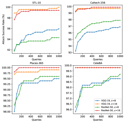
Figure 3: ASR vs. Queries under data-independent settings.

IV-D2 Model-independent Attack.

Existing black-box attack methods can only generate adversarial samples for a specific victim model. Our CDMA is not restricted by this requirement. It can synthesize adversarial examples by performing a conditional sampling manner, and we call it the model-independent attack. Specifically, in this situation, we don’t know what the victim model is but just do the conditional sampling once for the specific dataset, and then verify whether these sampled examples are adversarial or not. Figure 4 shows that the average success rate of such attack on CIFAR-10 is higher than 80% over different victim models. It can also achieve a 60+% average attack success rate on CIFAR-100 and Tiny-ImageNet. This phenomenon demonstrates that even in model-independent attack scenarios, CDMA can still generate adversarial examples and achieve good attack effects on different models. Furthermore, it illustrates the high adaptability of CDMA in model-independent black-box scenarios.

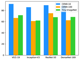
Figure 4: Model-independent attack.

IV-E Transfer Attack Effectiveness

Recall that the transferability of adversarial examples is crucial to carry out transfer attacks, especially for the black-box model deployed in the real world. Therefore following the previous works [8, 45], we examine the transferability of the generated AE for each of the attack methods in Table. VII. We randomly sample 1000 images from CIFAR-10, CIFAR-100 and Tiny-ImageNet datasets, and generate AEs against on ResNet-50 model. Then we transfer these AEs to attack the VGG-19, Inception V3 and DenseNet-169. As seen, the generated AE by CDMA transfer to other models easier than other attacks. This observation precisely matches our intuition about the mechanics of CDMA. More specifically, we know that in CDMA the model is learning a transformation between a benign image and its adversarial counterpart. Comparing to other queries and optimization attacks, which calculate specific perturbations for each sample, CDMA learns to use the transformation to build AEs. Thus, CDMA tends to generate AEs with high transferability.

TABLE VII: Transfer attack on different models.

	Methods	$\epsilon$=8			$\epsilon$=16
		VGG	Inception	DenseNet	VGG	Inception	DenseNet
CIFAR-10	AdvFlow	21.58	9.82	10.78	15.75	9.43	11.89
	RayS	14.74	7.38	12.74	23.53	9.76	15.00
	bayes_attack	24.24	34.38	28.01	51.44	47.54	59.10
	TA	21.15	8.77	19.30	23.05	26.47	24.91
	NPAttack	12.05	18.84	19.08	21.94	30.03	29.49
	ODS	50.86	45.94	53.18	49.12	43.61	50.22
	GFCS	55.92	49.19	55.33	54.76	51.03	57.45
	CG-Attack	57.64	48.28	56.18	61.93	58.67	62.79
	MCG-Attack	53.73	46.91	53.17	58.62	52.96	61.45
	CDMA	82.43	76.06	87.13	98.06	95.21	98.51
CIFAR-100	AdvFlow	12.74	5.59	15.30	14.93	11.48	12.83
	RayS	23.20	9.94	13.90	28.08	13.52	18.09
	bayes_attack	51.39	52.40	40.04	79.86	79.13	71.89
	TA	22.61	26.54	24.93	45.12	39.01	30.24
	NPAttack	39.81	41.38	35.37	60.00	58.84	54.07
	ODS	50.78	39.65	41.76	54.49	37.96	37.54
	GFCS	68.57	48.51	52.17	65.83	49.53	53.24
	CG-Attack	61.73	55.49	59.47	62.94	58.62	60.49
	MCG-Attack	58.61	53.97	58.63	58.46	53.61	56.37
	CDMA	71.74	60.96	68.55	89.57	82.12	87.71
Tiny-ImageNet	AdvFlow	8.82	5.75	12.03	8.56	7.06	12.37
	RayS	15.97	12.72	18.49	23.80	20.70	20.11
	bayes_attack	31.84	30.41	46.27	63.25	64.43	72.12
	TA	18.72	24.40	26.98	35.37	28.72	35.80
	NPAttack	12.78	13.64	18.53	16.25	17.38	25.28
	ODS	44.49	31.58	42.20	47.04	27.89	42.16
	GFCS	63.27	43.28	57.32	64.60	47.37	60.60
	CG-Attack	58.61	46.94	57.37	60.98	52.61	59.16
	MCG-Attack	57.92	44.28	54.37	61.94	53.63	58.61
	CDMA	76.36	68.22	86.46	90.33	84.31	95.82

IV-F Ablation Study

IV-F1 Scheduling & Steps.

Although the typical training and sampling steps of DDPM are $T=1000$, previous work [26] shows that such number of steps for the diffusion model can be inconsistent. Here, we aim to explore the effect of the number of sampling steps $T$ on the final attack performance without other acceleration schemes [46, 47]. The victim model is ResNet-50, the noise budget is set as $\epsilon=8$ and $\epsilon=16$, and the maximal number of queries is set as $Q=10$.

As shown in Figure 5, the obtained attack success rate always fluctuates regardless of using cosine or linear sampling. Compared with liner sampling, cosine sampling can achieve a higher attack success rate with fewer sampling steps. Especially when the number of sampling steps is small, the attack success rate of linear sampling is relatively lower. For example, when the number of sampling steps is $t=10$, the attack success rate of linear sampling is around 40%-60%, while the cosine sampling is 80%-90%. Note that for each sampling schedule, the final attack success rate is roughly the same as the number of sampling steps increases. To obtain more effective and efficient attack results, we set the sampling strategies in the attack process as follows: the sampling schedule is cosine and the number of steps is $t=50$. By doing this, the attack effectiveness is significantly promoted owning to a smaller sample step $t$.

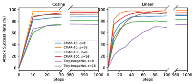
Figure 5: The attack performance v.s. different sample schedules under multiple sample steps.

IV-F2 Comparisons with Generative Attacks

Existing generative-based attacks usually use GAN to generate adversarial perturbations. We choose the most representative one, AdvGAN, among these methods to compare with our CDMA. As the experimental results are illustrated in Figure 6, we can find that although the attack success rate of our method is lower than AdvGAN in some cases, as the number of queries increases, the attack success rate of our method will increase with the number of queries, on the contrary, AdvGAN will not, which thoroughly verifies our assertion that the AEs generated by our CDMA can generate diversiform adversarial examples, even for the same clean example $x$.

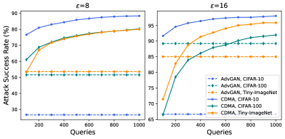
Figure 6: Queries vs. ASR of AdvGAN and CDMA on three different datasets.

V Conclusions

In this work, we find that adversarial examples are a particular form of benign examples, i.e., these two types of samples come from two distinct but adjacent distributions that can be transformed from each other with a perfect converter. Based on this observation, we propose a novel hard-label black-box attack, CDMA, which builds a converter to transform clean data to its corresponding adversarial counterpart. Specifically, we leverage a diffusion model to formulate the data converter and synthesize adversarial examples by conditioning on clean images to improve the query efficiency significantly. Extensive experiments demonstrate that CDMA achieves a much higher attack success rate within 1,000 queries and needs fewer queries to achieve the attack results, even in the targeted attack setting. Besides, most adversarial examples generated by CDMA can escape from mainstream defense strategies and maintain high robustness. Furthermore, CDMA can generate adversarial examples that are well transferred to different victim models or datasets.

Acknowledgements This work is supported in part by Yunnan Province Education Department Foundation under Grant No.2022j0008, in part by the National Natural Science Foundation of China under Grant 62162067 and 62101480, Research and Application of Object Detection based on Artificial Intelligence, in part by the Yunnan Province expert workstations under Grant 202205AF150145.

References

- [1] J. Chen, L. Yang, L. Tan, and R. Xu, “Orthogonal channel attention-based multi-task learning for multi-view facial expression recognition,” Pattern Recognition, vol. 129, p. 108753, 2022.
- [2] G. Li, Y. Zhang, D. Ouyang, and X. Qu, “An improved lightweight network based on yolov5s for object detection in autonomous driving,” in ECCV, vol. 13801, 2022, pp. 585–601.
- [3] X. Zhang, Y. Han, W. Xu, and Q. Wang, “HOBA: A novel feature engineering methodology for credit card fraud detection with a deep learning architecture,” Information Sciences, vol. 557, pp. 302–316, 2021.
- [4] N. Carlini and D. A. Wagner, “Towards evaluating the robustness of neural networks,” in S&P, 2017.
- [5] T. Combey, A. Loison, M. Faucher, and H. Hajri, “Probabilistic jacobian-based saliency maps attacks,” Machine Learning and Knowledge Extraction, vol. 2, no. 4, pp. 558–578, 2020.
- [6] I. J. Goodfellow, J. Shlens, and C. Szegedy, “Explaining and harnessing adversarial examples,” in ICLR, 2015.
- [7] J. Chen and Q. Gu, “Rays: A ray searching method for hard-label adversarial attack,” in KDD, 2020, pp. 1739–1747.
- [8] H. M. Dolatabadi, S. M. Erfani, and C. Leckie, “Advflow: Inconspicuous black-box adversarial attacks using normalizing flows,” in NeurIPS, 2020.
- [9] S. N. Shukla, A. K. Sahu, D. Willmott, and J. Z. Kolter, “Simple and efficient hard label black-box adversarial attacks in low query budget regimes,” in KDD, 2021, pp. 1461–1469.
- [10] X. Wang, Z. Zhang, K. Tong, D. Gong, K. He, Z. Li, and W. Liu, “Triangle attack: A query-efficient decision-based adversarial attack,” in ECCV, vol. 13665, 2022, pp. 156–174.
- [11] Y. Bai, Y. Wang, Y. Zeng, Y. Jiang, and S. Xia, “Query efficient black-box adversarial attack on deep neural networks,” Pattern Recognition, vol. 133, p. 109037, 2023.
- [12] W. Brendel, J. Rauber, and M. Bethge, “Decision-based adversarial attacks: Reliable attacks against black-box machine learning models,” in ICLR, 2018.
- [13] A. Ilyas, L. Engstrom, and A. Madry, “Prior convictions: Black-box adversarial attacks with bandits and priors,” in ICLR, 2019.
- [14] S. B. Shah, P. Raval, H. Khakhi, and M. S. Raval, “Frequency centric defense mechanisms against adversarial examples,” in MM, 2021, pp. 62–67.
- [15] W. Nie, B. Guo, Y. Huang, C. Xiao, A. Vahdat, and A. Anandkumar, “Diffusion models for adversarial purification,” in ICML, vol. 162, 2022, pp. 16 805–16 827.
- [16] J. Wang, Z. Lyu, D. Lin, B. Dai, and H. Fu, “Guided diffusion model for adversarial purification,” CoRR, vol. abs/2205.14969, 2022.
- [17] N. Papernot, P. D. McDaniel, I. J. Goodfellow, S. Jha, Z. B. Celik, and A. Swami, “Practical black-box attacks against machine learning,” in Asia@CCS, 2017, pp. 506–519.
- [18] Z. Huang and T. Zhang, “Black-box adversarial attack with transferable model-based embedding,” in ICLR, 2020.
- [19] Y. Tashiro, Y. Song, and S. Ermon, “Diversity can be transferred: Output diversification for white- and black-box attacks,” in NeurIPS, 2020.
- [20] N. A. Lord, R. Müller, and L. Bertinetto, “Attacking deep networks with surrogate-based adversarial black-box methods is easy,” in ICLR, 2022.
- [21] Y. Feng, B. Wu, Y. Fan, L. Liu, Z. Li, and S. Xia, “Boosting black-box attack with partially transferred conditional adversarial distribution,” in CVPR, 2022, pp. 15 074–15 083.
- [22] P. Chen, H. Zhang, Y. Sharma, J. Yi, and C. Hsieh, “ZOO: zeroth order optimization based black-box attacks to deep neural networks without training substitute models,” in AISec@CCS, 2017, pp. 15–26.
- [23] J. Ho, A. Jain, and P. Abbeel, “Denoising diffusion probabilistic models,” in NeurIPS, 2020.
- [24] O. Ronneberger, P. Fischer, and T. Brox, “U-net: Convolutional networks for biomedical image segmentation,” in MICCAI, vol. 9351, 2015, pp. 234–241.
- [25] A. Madry, A. Makelov, L. Schmidt, D. Tsipras, and A. Vladu, “Towards deep learning models resistant to adversarial attacks,” in ICLR, 2018.
- [26] C. Saharia, W. Chan, H. Chang, C. A. Lee, J. Ho, T. Salimans, D. J. Fleet, and M. Norouzi, “Palette: Image-to-image diffusion models,” in SIGGRAPH, 2022, pp. 15:1–15:10.
- [27] J. Choi, S. Kim, Y. Jeong, Y. Gwon, and S. Yoon, “ILVR: conditioning method for denoising diffusion probabilistic models,” in ICCV, 2021, pp. 14 347–14 356.
- [28] A. Krizhevsky and G. Hinton, “Learning multiple layers of features from tiny images,” Computer Science Department, University of Toronto, Tech. Rep, vol. 1, 01 2009.
- [29] J. Deng, W. Dong, R. Socher, L. Li, K. Li, and L. Fei-Fei, “Imagenet: A large-scale hierarchical image database,” in CVPR, 2009, pp. 248–255.
- [30] K. Simonyan and A. Zisserman, “Very deep convolutional networks for large-scale image recognition,” in ICLR, 2015.
- [31] C. Szegedy, V. Vanhoucke, S. Ioffe, J. Shlens, and Z. Wojna, “Rethinking the inception architecture for computer vision,” in CVPR, 2016, pp. 2818–2826.
- [32] C. Szegedy, S. Ioffe, V. Vanhoucke, and A. A. Alemi, “Inception-v4, inception-resnet and the impact of residual connections on learning,” in AAAI, 2017, pp. 4278–4284.
- [33] K. He, X. Zhang, S. Ren, and J. Sun, “Deep residual learning for image recognition,” in CVPR, 2016, pp. 770–778.
- [34] G. Huang, Z. Liu, L. van der Maaten, and K. Q. Weinberger, “Densely connected convolutional networks,” in CVPR, 2017, pp. 2261–2269.
- [35] F. Yin, Y. Zhang, B. Wu, Y. Feng, J. Zhang, Y. Fan, and Y. Yang, “Generalizable black-box adversarial attack with meta learning,” CoRR, vol. abs/2301.00364, 2023.
- [36] R. Shin and D. Song, “Jpeg-resistant adversarial images,” in NeurIPS, vol. 1, 2017, p. 8.
- [37] M. Naseer, S. H. Khan, M. H. Khan, F. S. Khan, and F. Porikli, “Cross-domain transferability of adversarial perturbations,” in NeurIPS, 2019, pp. 12 885–12 895.
- [38] A. Prakash, N. Moran, S. Garber, A. DiLillo, and J. A. Storer, “Deflecting adversarial attacks with pixel deflection,” in CVPR, 2018, pp. 8571–8580.
- [39] “Improved robustness to adversarial examples using lipschitz regularization of the loss,” CoRR, vol. abs/1810.00953, 2018.
- [40] W. Xu, D. Evans, and Y. Qi, “Feature squeezing: Detecting adversarial examples in deep neural networks,” in NDSS, 2018.
- [41] A. Coates, A. Y. Ng, and H. Lee, “An analysis of single-layer networks in unsupervised feature learning,” in AISTATS, ser. JMLR Proceedings, vol. 15, 2011, pp. 215–223.
- [42] L. Fei-Fei, R. Fergus, and P. Perona, “Learning generative visual models from few training examples: An incremental bayesian approach tested on 101 object categories,” computer vision and image understanding, vol. 106, no. 1, pp. 59–70, 2007.
- [43] B. Zhou, A. Lapedriza, A. Khosla, A. Oliva, and A. Torralba, “Places: A 10 million image database for scene recognition,” IEEE Transactions on Pattern Analysis and Machine Intelligence, 2017.
- [44] Z. Liu, P. Luo, X. Wang, and X. Tang, “Deep learning face attributes in the wild,” in ICCV, 2015, pp. 3730–3738.
- [45] P. Zhao, P. Chen, S. Wang, and X. Lin, “Towards query-efficient black-box adversary with zeroth-order natural gradient descent,” in AAAI, 2020, pp. 6909–6916.
- [46] L. Liu, Y. Ren, Z. Lin, and Z. Zhao, “Pseudo numerical methods for diffusion models on manifolds,” in ICLR, 2022.
- [47] R. Rombach, A. Blattmann, D. Lorenz, P. Esser, and B. Ommer, “High-resolution image synthesis with latent diffusion models,” in CVPR, 2022, pp. 10 674–10 685.