The Quantum Transition of the Two-Dimensional Ising Spin Glass: A Tale of Two Gaps
Abstract
Quantum annealers are commercial devices aiming to solve very hard computational problems Johnson et al. (2011) named spin glasses Charbonneau et al. (2023). Just like in metallurgic annealing one slowly cools a ferrous metal Kirkpatrick et al. (1983), quantum annealers seek good solutions by slowly removing the transverse magnetic field at the lowest possible temperature. The field removal diminishes quantum fluctuations but forces the system to traverse the critical point that separates the disordered phase (at large fields) from the spin-glass phase (at small fields). A full understanding of this phase transition is still missing. A debated, crucial question regards the closing of the energy gap separating the ground state from the first excited state. All hopes of achieving an exponential speed-up, as compared to classical computers, rest on the assumption that the gap will close algebraically with the number of qspins Rieger and Young (1994); Guo et al. (1994); Rieger and Young (1996); Singh and Young (2017), but renormalization group calculations predict that the closing will be instead exponential Miyazaki and Nishimori (2013). Here we solve this debate through extreme-scale numerical simulations, finding that both parties grasped parts of the truth. While the closing of the gap at the critical point is indeed super-algebraic, it remains algebraic if one restricts the symmetry of possible excitations. Since this symmetry restriction is experimentally achievable (at least nominally), there is still hope for the Quantum Annealing paradigm Kadowaki and Nishimori (1998); Brooke et al. (1999); Farhi et al. (2001).
I Introduction
Optimization problems are ubiquitous in everyday life (think, for instance, of deciding the best delivery route, or deciding assignments in the national budget). These problems can be mathematically formalized: agents (e.g. ministries seaking their part in the budget) compete, trying to satisfy their mutually contradicting goals. The overall frustration produced by a particular solution is quantified through a cost function, that we attempt to minimize. This task is best solved with the help of a computer, even for quite small . Computational complexity studies how the computational resources (memory, computing time, etc.) grow with Papadimitriou (1994). If, for all known algorithms, the necessary resources grow faster with than any polynomial, e.g. like , the problem is considered hard. A small subset of these problems, named NP-complete, is of particular interest: if an efficient algorithm (i.e. resources scaling polynomially in ) were discovered for any of the NP-complete problems, then a vast family of hard optimization problems would become easy. For physicists, the most familiar example of a NP-complete problem is finding the minimal energy state —the Ground state (GS)— of an Ising spin-glass Hamiltonian on a non-planar graph Barahona (1982); Istrail (2000). This explains the up-surge of hardware specifically designed for minimizing a spin-glass Hamiltonian through a variety of algorithms and/or physical principles (see e.g Goto et al. (2019); Matsubara et al. (2020); McGeoch and Farré (2020); McMahon et al. (2016); Baity-Jesi et al. (2014)).
Specifically, the strategy that concerns us here is Quantum Annealing. Both in the original formulation Kadowaki and Nishimori (1998), and also in its hardware implementation Johnson et al. (2011); McGeoch and Farré (2020), people aim at solving spin glasses. In particular, D-wave chips solve Ising spin glass in space dimension ( can be coded over D-wave’s graph King et al. (2023); see Baxter (2008) for more on the definition of ).
The spin glass is the paradigmatic statistical model for quenched disorder Parisi (1994). The Hamiltonian for spins (or qspin) is
| (1) |
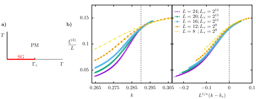
where the are the random couplings that define the problem instance under consideration, is the transverse field and and are, respectively, the first and third Pauli matrices acting on the spin that lies in site . The phase diagram for a two-dimensional interaction matrix is sketched in Fig. 1–(a). For , the GS has all spins as much aligned with the transverse field as Quantum Mechanics allows them to be (paradoxically enough, from the point of view of the computational basis that diagonalizes the matrices, this GS seems a totally random statistical mixture). As is diminished at zero temperature, the GS varies. In particular, at , the GS encodes the solution of the Optimization problem we are interested in. At some point along the annealing, goes through the critical value that separates the disordered GS from the spin-glass GS that does show a glassy order in the computational basis. This is not just theorist daydreaming. In a recent experiment conducted on a D-wave chip King et al. (2023), some 5000 qubits displayed coherent quantum dynamics as went through , for annealings lasting several nanoseconds.
A strong theoretical command on the phase transition at is clearly necessary. A very powerful tool in the analytical study of phase transitions is the Renormalization Group (RG), which helps to clarify which properties of the critical point are not modified by microscopic details in which different experiments may differ. Only very broad features, such as symmetries, matter (making it possible to classify problems into universality classes). In fact, the study of disordered systems was one of the early applications of the RG group (see, e.g., Refs. Grinstein and Luther (1976); Parisi (1979); Parisi and Sourlas (1979)), a strategy that is firmly established in Cardy (1996). Yet, it has taken considerable time and effort to show that the RG —and the accompanying universality— applies to disordered systems in as well Ballesteros et al. (1998); Hasenbusch et al. (2008); Fytas and Martín-Mayor (2013); Fytas et al. (2016, 2019) (even in this was a hard endeavor for spin glasses Fernandez et al. (2016)). Unfortunately, the study of the quantum spin-glass transition at finite is a lot behind its thermal counterpart. Essentially, only the case is well understood McCoy and Wu (1968); McCOY and WU (1969); McCOY (1969); Fisher (1992).
The second-simplest problem to analyze, the spin glass in , poses quite a challenge. Indeed, different approaches have produced mutually contradicting predictions for the crucial physical quantity that will ultimately decide whether or not the quantum computational complexity of the problem to be considered is smaller than its classical counterpart. We are referring to the energy gap that separates the GS from the first excited state of the Hamiltonian (1). Indeed, the required annealing time is proportional to . In a spin glass with qspins at ( is the linear size of the system), ( is the so called dynamic critical exponent). Early Monte Carlo simulations Rieger and Young (1994); Guo et al. (1994); Rieger and Young (1996) and a series-expansion study Singh and Young (2017) found finite values of (e.g., for spin glasses Rieger and Young (1994)). A finite is also a crucial assumption of the droplet model for the quantum spin glass transition Thill and Huse (1995). On the other hand, a real-space RG analysis concludes in space dimension and Miyazaki and Nishimori (2013) (a Monte Carlo simulation claims as well in Matoz-Fernandez and Romá (2016)).
The starting assumption of Refs. Rieger and Young (1994); Guo et al. (1994); Rieger and Young (1996); King et al. (2023) was a finite value of exponent . Yet, to clarify the aforementioned controversy, our analysis will be completely agnostic about . Just as Rieger and Young pushed to their very limit the computational capabilities at that time by using special hardware (Transputers) Rieger and Young (1994), we have performed unprecedented large scale simulations on GPUs by using highly tuned custom codes. A careful consideration of the global spin-flip symmetry, implemented by the parity operator , turns out to be crucial to clarify the situation.
II The Ground State
Our aim here is studying the phase transition as seen from the GS (so that the spectra of excitations, and hence exponent , does not play any role in the analysis in Sect. II.2). This entails taking the limit .
In the Trotter formulation that we use (see Methods), the original qspins on a lattice are replaced by classical spins on a lattice, . The extra dimension is named the Euclidean time. is replaced by a new parameter , that grows as decreases. An energy gap translates into a correlation length along the Euclidean time. In this formulation, the limits and are equivalent.
Although our main results stem from Monte Carlo simulations, a complementary exact diagonalization effort on small systems —see Sect. II.1 and Methods— has being extremely useful both to shape our analysis, and to understand how the limit is approached (Sect. II.3).
II.1 Exact diagonalization
The main lessons that exact diagonalization of systems with size have taught us are the following.
The parity operator splits the spectrum of the Hamiltonian (1) into even energy levels () and odd levels (). The GS is even and its energy is .
The first excited state is . The minimal gap displays dramatic fluctuations among samples, up to the point that the statistical analysis should be conducted in terms of . Furthermore, varies significantly with . Instead, the sample-to-sample fluctuations of the same-parity gaps, and are very mild (also their -dependence is mild). For all our samples, and are of similar magnitude and, unless turns out to be inordinately large, .
Thermal expected values of even operators (i.e., operators such that ) reach their limit for a surprisingly small values of . The reasons explaining this benign behavior are understood, see Methods.
II.2 The phase transition
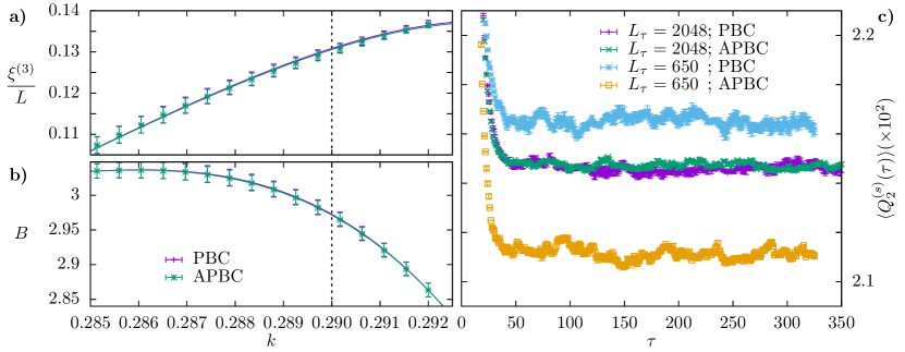
The standard spin-glass correlation function, when computed on the GS (see Methods), is afflicted by a very large anomalous dimension that makes the spin-glass susceptibility barely divergent at the critical point Rieger and Young (1994). We have circumvented this problem by considering instead, the correlation matrix (see Methods and Refs. Yang (1962); Sinova et al. (2000); Correale et al. (2002)). From , one can compute not only , but also a better behaved susceptibility . The corresponding correlation length is suitable for a standard Finite-Size scaling study of the phase transition, see e.g. Amit and Martín-Mayor (2005), that is illustrated in Figs. 1–(b).
The analysis in Methods finds for the critical point , the correlation-length exponent and exponents []:
| (2) | |||||
| (3) |
The first error estimate is statistical whereas the second error accounts for systematic effects (see Methods) Note that the bound Chayes et al. (1986) is verified, and that is, indeed, barely divergent Rieger and Young (1994).
II.3 On the limit of zero temperature
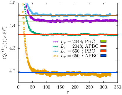
The naive approach to the limit would be studying a fixed set of samples for a sequence of growing Euclidean lengths and check when the results become independent (indeed, effects die out as ). However, on the view of Sect. II.1, this is just a wishful thinking. Indeed, some instances have an inordinately small gap (hence a huge Euclidean correlation length ), and so for all the values of that we can simulate (one wishes to have , instead).
Fortunately, considering simultaneously periodic and anti-periodic boundary conditions (PBC and APBC, respectively) along the Euclidean time offers a way out. The detailed analysis in Methods shows that the sequence of results for growing converges to from opposite sides. As grows, see Fig. 2-(c), the PBC sequence monotonically decreases, while the APBC sequence increases. Thus, statistical compatibility for both boundary conditions ensures that the zero-temperature limit has been reached.
III Spectra of excitations at the transition
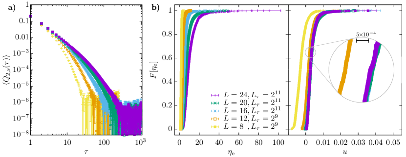
The main tool to investigate excitations is the dependence of the Euclidean correlation function of several operators, see Methods. It will be crucial to distinguish even operators (i.e. ) from odd operators (). For even operators, the decay with is sensitive only to same-parity gaps (such as and defined in Sect. II.1). Instead, odd operators feel the different-parity energy gap .
For both symmetry sectors, the correlation functions computed in a sample decay exponentially (to zero in the case of odd operators or, Fig. 2–c, to a plateaux for even operators). In both cases, correlation lengths and the energy gaps of appropriate symmetry are related as . Therefore, what the average over samples of an Euclidean correlation function really features is the probability distribution function (as computed over the different samples) of the correlation lengths .
From now on, we specialize to the critical point at .
III.1 Even operators
This case is of utmost relevance because only even excited states may cause the system to leave its GS in an (ideal) quantum annealing for the Hamiltonian (1). Our approach is not entirely satisfying in this respect because, for a given sample, we obtain the smallest of the two same-parity gaps and (one would like to study only ). Fortunately, see Methods, both gaps are of similar magnitude.
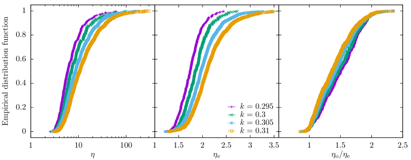
The first optimistic indication comes from the (substracted) correlation function in Fig 3–a that indeed goes to zero (within errors) for a moderate value of . Indeed, the empirical distribution function for the correlation length in Fig 3–b indicates mild sample-to-sample fluctuations and a relatively weak dependence on . Indeed, as shown Fig 3–b, for all , the probability distribution function turns out to depend on the scaling variable
| (4) |
(Setting , the whole curve cannot be made to scale and the resulting estimate is lower). Thus, as anticipated, we conclude that the even symmetry sector shows algebraic scaling for its gap.
III.2 Odd operators
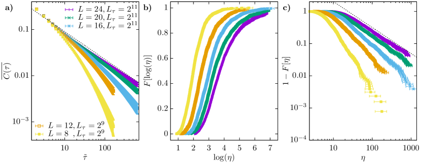
As it could be expected from the exact results in McCoy and Wu (1968); McCOY (1969); Fisher (1992) and the approximate Renormalization Group for Miyazaki and Nishimori (2013), the odd correlation function in Fig. 4–a displays, for large , a power law decay with . This implies that the magnetic susceptibility —the linear response to a magnetic field aligned with the Z axis— is divergent at the critical point. Indeed, the susceptibility diverges if (because it is twice the integral of for going from to ).
Furthermore, also for , see Methods. We therefore conclude that the susceptibility is divergent in the paramagnetic phase. This is exactly the same behaviour encountered in . Accordingly, the probability distribution function of the Euclidean correlation length —recall that — displays a extremely fat tail, see Figs. 4–b and 4–c. We are in the presence of a Levy flight, which strongly suggests that the scenario of an infinite-randomness fixed-point Miyazaki and Nishimori (2013) is, indeed, realized for the Ising spin glass.
IV Conclusions and Outlook
We have solved a decades-long controversy through an extreme-scale simulation on GPUs, and a careful consideration of the main symmetries of the problem. Our main conclusion is very optimistic: there is no objection of principle impeding a quantum annealer to remain in the ground state while entering the spin-glass phase, recall Fig. 1–(a). However, as discussed below, this is not quite the same as solving our optimization problem. In order to adiabatically enter the spin-glass phase, the annealing time would just need to grow as a power-law with the number of qspins, recall Eq. (4), provided that parity-changing excitations are avoided (something that, at least nominally, is within the capabilities of current hardware). Universality and the Renormalization Group suggest that this optimistic conclusion extends to a vast family of problems (all problems that share the space-dimension and the basic symmetries with our spin glass on the square lattice).
However, our findings pose as well many questions. Let us list a few.
We have seen that entering the spin-glass phase with a quantum annealer should be doable with an effort polynomial in the number of qbits. However, in order to solve an optimization problem, one still needs to go adiabatically all the way from the critical point to . This is a difficult journey, at least for problems with space dimension Knysh (2016). However, it has been recently argued that an algebraic speed-up, as compared to classical algorithms, is within reach King et al. (2023). Having a finite exponent is a basic prerequisite also for algebraic speed-up.
We know that Ising glasses may be both hard and easy to solve on a classical computer. For instance, problems formulated in the square lattice with nearest-neighbor interactions can be solved quite efficiently (see, e.g., Khoshbakht and Weigel (2018)). However, adding second-neighbor interactions results into a NP-complete problem. As far as we know, it is still unclear whether or not these two problems belong to the same (quantum) computational complexity-class. Since the second-neighbor interactions should play no role at , differences between the two kind of problems (if any) should arise for transverse fields .
In this work, we have chosen problem instances with uniform probability, but this is not a necessity. One could focus, instead, on samples that are particularly hard to solve with a classic digital computer Fernandez et al. (2013); Marshall et al. (2016); Billoire et al. (2018). It would be interesting to test if the benign scaling in Eq. (4) remains unchanged under these challenging circumstances. We know that these classically hard problems are even harder to solve in a D-wave’s annealer Martín-Mayor and Hen (2015), but there are many possible explanations for this poor performance of quantum hardware (see,e.g., Albash et al. (2017, 2019)).
Another possible venue of research is concerned with three dimensional systems. A recent experiment conducted on D-wave hardware suggests King et al. (2023). Whether this finite dynamic exponent refers only to even excitations (as it would be the case in two dimensions) or it is unrestricted Guo et al. (1994) is, probably, worthy of investigation.
Acknowledgements.
We thank Antonello Scardicchio for useful discussions. We also thank Andrew King for a most useful correspondence. We benefited from two EuroHPC computing grants: specifically, we had access to the Meluxina-GPU cluster through grant EHPC-REG-2022R03-182 (158306.5 GPU computing hours) and to the Leonardo facility (CINECA) through a LEAP grant ( GPU computing hours). Besides, we received a small grant (10000 GPU hours) from the Red Española de Supercomputación, through contract no. FI-2022-2-0007. Finally we thank Gianpaolo Marra for the access to the Dariah cluster in Lecce. This work was partially supported by Ministerio de Ciencia, Innovación y Universidades (Spain), Agencia Estatal de Investigación (AEI, Spain, 10.13039/501100011033), and European Regional Development Fund (ERDF, A way of making Europe) through Grant PID2022-136374NB-C21. This research has also been supported by the European Research Council under the European Unions Horizon 2020 research and innovation program (Grant No. 694925—Lotglassy, G. Parisi). IGAP was supported by the Ministerio de Ciencia, Innovación y Universidades (MCIU, Spain) through FPU grant No. FPU18/02665.Conflict of interests
The authors declare no conflict of interests.
Authors’ contributions
G.P. suggested to undertake this project. M.B., I.G.-A.P. and V.M.-M. planned research. M.B., I.G.-A.P., V.M.-M., and G.P. contributed computer code. M.B. and I.G.-A.P. carried out the simulations. M.B., I.G.-A.P., V.M.-M., and G.P. analyzed the data and wrote the paper.
Availability of data
Data can be obtained from the corresponding author (I.G.-A.P.) upon reasonable request.
Code availability
The authors will make their code publicly available through a separate publication. Meanwhile, upon reasonable request, the code can be obtained from M.B.
Appendix A Methods
A.1 Model and simulations
Our qspins occupy the nodes of a square lattice of side , endowed with periodic boundary conditions. The coupling matrix in Eq. (1) is non-vanishing only for nearest lattice-neighbors. A problem instance, or sample, is defined by the choice of the matrix. The non-vanishing matrix elements, are random, independent variables in our simulations. Specifically, we chose with probability. We chose energy units such that .
Given an observable , we shall refer to its thermal expectation value in a given sample as , see below Eq. (8) (the temperature is as low as possible, ideally ). Thermal expectation values are averaged over the choice of couplings (quenched disorder, see e.g. Parisi (1994)). We shall denote the second average —over disorder— as .
A.1.1 Crucial symmetries

The most prominent symmetries in this problem are the gauge and the parity symmetries. Both symmetries are exact for the Hamiltonian (1) and for its Trotter-Suzuki approximation (see Sect. A.1.2).
The parity symmetry is a self-adjoint, unitary operator that commutes with the Hamiltonian (1), as well as with the exact (7) and approximate (8) transfer matrices. The Hilbert space is divided into two sub-spaces of the same dimension, according to the parity eigenvalue, either (even states) or (odd states). We classify also operators as either even (i.e. ) or odd operators (). Matrix elements of even operators can be non-vanishing only if the two states have the same parity (on the contrary, for odd operators the parity of the states should differ). An oversimplified but enlightening cartoon of the spectra in our problem is represented in Fig. 5 (see below some exact-diagonalization results that support this view).
The parity symmetry is just a particular case of gauge transformation. Let us arbitrarily choose for each site or 1. The corresponding gauge operator is self-adjoint and unitary. It transforms the Hamiltonian in Eq. (1) in a Hamiltonian of the same type, but with modified couplings Toulouse (1977): The gauge symmetry is enforced by the process of taking the disorder average. Indeed, the gauge-transformed coupling matrix has the same probability as the original one. Hence, meaningful observables should be invariant under an arbitrary gauge transformation. The parity operator is obtained by setting for all sites, which does not modify the (hence, parity is a symmetry for a given problem instance not just a symmetry induced by the disorder average).
A.1.2 The Trotter-Suzuki formula
We follow the Trotter-Suzuki approximation Trotter (1959); Suzuki (1976) that replaces the original qspins on a lattice by classical spins on a lattice, . The extra dimension is named Euclidean time. We shall write as a shorthand for the spins in the system (, here). Instead, will refer to the spins at time . The probability of is given by
| (5) |
with [ in Eq. (5) is named the partition function]
Periodic boundary conditions (PBC) are assumed along the Euclidean time. Below, we shall find it useful to consider as well antiperiodic boundary conditions only along the direction (APBC). Besides, as the reader may check, is a monotonically decreasing function of .
Maybe the most direct connection between the classical spin system and the original quantum problem is provided by the transfer matrix Kogut (1979); Parisi (1988). Let us define and . The quantum thermal expectation value at temperature is
| (7) |
Now, for being an arbitrary function, the Trotter-Suzuki approximation amounts to substitute the true transfer matrix in Eq. (7) by its proxy []:
| (8) |
can be computed as well by averaging , evaluated over configurations distributed according to (5) (the value of is arbitrary, hence one may gain statistics by averaging over ).
Finally, let us emphasize that both and are self-adjoint, positive-define transfer matrices that share the crucial symmetries discussed in Sect. A.1.1.
A.2 Observables
The quantities defined in Sect. A.2.1 aim at probing the ground state as [and hence (A.1.2)] varies. These quantities will always be averaged over disorder before we proceed with the analysis.
Instead, the time correlations in Sect. A.2.2 will probe the excitations. These time correlations will be analyzed individually for each sample (sample-to-sample fluctuations are considered in Sect. A.5).
A.2.1 One-time observables
We consider the correlation matrices and Yang (1962); Sinova et al. (2000) — or :
| (9) |
The -body spin-glass susceptibilities at both zero and minimal momentum are
| (10) |
and give us access to the second-moment correlation length (see, e.g., Ref. Amit and Martín-Mayor (2005))
| (11) |
As grows, and remain of order 1 in the paramagnetic phase whereas, in the critical region, they diverge as and . In the spin-glass phase, ( with some unknown exponent ).
Our and are just the standard quantities in the spin-glass literature Palassini and Caracciolo (1999); Ballesteros et al. (2000). In fact, in the simplest approximation —see Ref. Correale et al. (2002) for a more paused exposition— at criticality and for large separations between and , with (so, in this approximation). Hence, if , grows with . Indeed, turns out to be a good compromise between statistical errors, that grow with , and a strong enough critical divergence of ( barely diverges Rieger and Young (1994)).
Besides, we have computed the Binder cumulant as ()
| (12) |
The Gaussian nature of the fluctuations in the paramagnetic phase causes to approach 3 as grows for fixed . reaches different large- limits for fixed (for different behaviors are possible, depending on the degree of Replica Symmetry Breaking Mézard et al. (1987)).
A.2.2 Two-times observables
Let us start by defining the time-correlation function of an observable (for simplicity, consider a product of operators at some sites):
| (13) |
can be computed from our spin configurations distributed according to the classical weight (5) by averaging (notations as in Sect. A.1.2).
Specifically, we have considered
| (14) |
Let us briefly recall some general results Kogut (1979); Parisi (1988) about , that follow from the spectral decomposition of the transfer matrix (to simplify notations, let us first disregard the parity symmetry and consider PBC).
The -dependence is given by the additive contribution of every pair of states ( is the Ground State). Every pair generates an exponentially decaying term with correlation length , . The amplitude is , with . Hence if the contribution of this pair of states can be neglected. Besides, in the presence of parity symmetry, for an even we find if the parity of and differ (for odd operators if both parities are equal). This is why the largest correlation length for is the maximum of and , whereas the relevant correlation length for is (recall Fig. 5).
Moreover, for even operators, every state provides an additive contribution to a -independent term (namely, the plateau in Fig. 6): . Instead, for odd operators (hence, odd operators lack a plateau). To manage the case of APBC, one just needs to add an extra parity operator as a final factor in both the numerator and the denominator of both Eqs. (8, 13). If parity is a symmetry, as is the case for our problem, is modified as ( is the parity of the state) and the contribution to the APBC plateau gets an extra factor , as well.
A.2.3 The limit of zero temperature
We shall assume that we can reach large enough to have (notations are explained in Fig. 5). Instead, we shall not assume that is small (in fact, for some samples one could even have ).
Now, consider an even operator , and let us define and (the thermal expectation value at exactly is ). The plateau at , see Fig. 6, is given ( for PBC and for APBC)
| (15) |
Thus, we get for the plateau of
| (16) |
where and are, respectively, the average over all pairs of and [, recall Eq. (14)]. To an excellent numerical accuracy, the l.h.s. of Eq. (16) is also the value one gets for , see Fig. 6. As a matter of fact, the difference between and its plateau is [hence, quadratic in rather than linear as in Eq. (15)].
First, the limit (or ) is approached monotonically. Furthermore, the systems with PBC and APBC [Fig. 6] approach the limit from opposite sides. We have explicitly checked all our samples, finding no instance where the APBC plateau lies above the PBC one (it is intuitively natural to expect that the PBC system will be more ordered than the APBC one). Hence, we conclude that the samples with PBC converge to from above, whereas the APBC ones converge from below.
Second, since is bounded between 0 and 1 also for APBC, we conclude that . Hence, quite paradoxically, the particularly difficult samples with generate a very small finite-temperature bias in the PBC estimator [compare the dependence of the PBC and the APBC plateaux in Fig. 6]. This is why we are able to reach the limit for the even operators, even if a fraction of our samples suffer from a large value of .
A.2.4 Simulation details
We have followed two approaches: exact diagonalization of the transfer matrix (8) and Markov Chain Monte Carlo simulations of the classical weight (5). GPUs were crucial for both. We provide here only the main details (the interested reader is referred to Bernaschi et al. (2023)).
Exact diagonalization is limited to small systems (up to in our case). Indeed, the transfer matrix has a size . Parity symmetry has allowed us to represent as a direct sum of two sub-matrices of half that size Bernaschi et al. (2023). Specifically, we have computed the eigenvalues , , , , as well as the corresponding eigenvectors , , , , for 1280 samples of at and (the same samples at both values). We repeated the calculations for a subset of 350 samples at and . We managed to keep the computing time within an acceptable time frame of 20 minutes per diagonalization using 256 GPU, thanks to a highly tuned custom matrix-vector product Bernaschi et al. (2023). These computations have proven to be invaluable in the process of taking the limit . (see Sect. A.3)
Our Monte Carlo simulations employed the Parallel Tempering algorithm Hukushima and Nemoto (1996), implemented over the parameter in (5), to ensure equilibration. We equilibrated 1280 samples of every of our lattice sizes (see Table 1). As a rule, we have estimated errors using the bootstrap method Efron and Tibshirani (1994), as applied to the disordered average.
We have simulated 6 real replicas of every sample (i.e. six statistically independent simulations of the system), for multiple reasons. Replicas allow us to implement the equilibration tests based on the tempering dynamics Billoire et al. (2018). They also provide unbiased estimators of products of thermal averages (10). Finally, fluctuations between replicas allow us to estimate errors for the time correlation functions (14), as computed in a single sample (see Sect. A.5).
The Monte Carlo code exploits a three-level parallelization (multispin coding, domain decomposition, parallel tampering) that allows keeping the spin-update time below 0.5 picoseconds Bernaschi et al. (2023), competitive with dedicated hardware Baity-Jesi et al. (2014).
| of | MC steps | ||||
|---|---|---|---|---|---|
A.3 Exact diagonalization
The schematic representation of the spectrum in Fig. 5 is based on the distribution functions in Figure 7 (we typically compute the inverse distribution function, see Sect. A.5 for details).
Indeed, see Fig. 7-a, the correlation length displays very large sample-to-sample fluctuations (to the point that a logarithmic representation is advisable) and a very strong -dependence. Instead, is always a number of order one in our samples (Fig. 7-b). Furthermore, Fig. 7-c, in all cases.
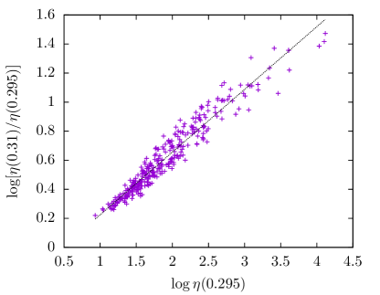
In fact, recall Fig. 4-c, the distribution for is a Levy flight [i.e. for large , ]. The mechanism allowing exponent to vary with [hence with transverse field (A.1.2)] is sketched in Fig. 8. Let us compare the value of for the same sample at and (). With great accuracy, , where are constants (for fixed and ) and . This monotonic relation implies that the same sample occupies percentile in the distribution for both and . It follows that for the exponent characterizing the Levy flight. In other words, because , the tail at large becomes heavier as increases (see Sect. A.6 for an extended discussion).
A.4 The critical point and critical exponents
After taking care of the limit (within errors), in our study of the phase transition, we still need to cope with the finite spatial dimension . We shall do so using Finite-Size scaling Fisher and Ferdinand (1967); Fisher and Barber (1972); Barber (1983); Cardy (2012) (see Fig. 1-c). The main questions we shall address are the computation of the critical exponents and the estimation of the critical point. Our main tool will be the quotients method Nightingale (1976); Ballesteros et al. (1996); Amit and Martín-Mayor (2005) that, surprisingly, keeps somewhat separate our two questions.
The quotients method starts by comparing a dimensionless quantity at two sizes (in our case, as a function of ). First, we locate a coupling such that the curves for and cross, see Fig. 1-b. Now, for dimensionful quantities , scaling in the thermodynamic limit as , we consider the quotient at . Barring scaling corrections, which yields an effective estimate of . Indeed, considering only the leading correction to the scaling exponent, , we have for the effective exponent
| (17) |
where is an amplitude. Our estimates for the effective exponents can be found in Table 2. Yet, effective exponents need to be extrapolated to the thermodynamic limit through Eq. (17). Unfortunately, we have not been able to estimate exponent (there were two difficulties: first, the range of values at our disposal was small, second the analytic background Amit and Martín-Mayor (2005) for the observables and for the Binder parameter —Sect. A.2.1— compete with the corrections). Hence, we have followed an alternative strategy. We have fitted our effective exponents to Eq. (17) with fixed (the fit parameters were the extrapolated and the amplitude . To account for our ignorance about , we made it vary in a wide range . The central values in Eqs. (2, 3) were obtained with , whereas the second error estimate accounts for the -dependence of the . As for the first error estimate, it is the statistical error as computed for . To take into account data we employed a bootstrap method Yllanes (2011). We considered only the diagonal part of the covariance matrix in the fits, performing a new fit for every bootstrap realization. Errors were computed from the fluctuations of the fit parameters. Fortunately, systematic errors turned out to be comparable (for smaller) with the statistical ones.
As for the critical point, one expects scaling corrections of the form ( is an amplitude) Binder (1981):
| (18) |
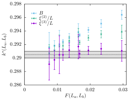
Unfortunately, this result is not of much use without a estimate. Fortunately, see Table 2 and Fig. 9, the values of obtained from seem not to depend on size. In fact, our estimate for in Eq. (2) is an interval that encompasses all our results (the shaded area in Fig. 9). Furthermore, the crossing points for and , see Fig. 9, seem also reasonably well represented by Eq. (18).
A.5 Fitting process and Euclidean correlation length estimation
Our aim here is to determine the relevant correlation-lengths for and at a fixed , for our samples. The results will be characterized through their empirical distribution function, recall Figs. 3 and 4. Given that is large, we need an automated approach.
The first step is estimating, for a given sample, and , as well as their standard errors, by using our 6 replicas. Now, the analysis of a noisy correlation function [such as and —see, e.g., Fig. 6] needs a fitting window Sokal (1997); Belletti et al. (2008). We chose the window upper limit as , with either or ( is the plateau, see Fig. 6), and the corresponding standard error. We need to face two problems. First, for the odd some samples have . For these samples, , and hence it is impossible to estimate, see Fig. 4-b. is not afflicted by this problem, see Fig.3. Second, we need to estimate the plateau . To do so, we fit for to a constant . In the few exceptions where this fit was not acceptable (as determined by its figure of merit computed with the diagonal part of the covariance matrix), we proceeded as explained below (we used in those cases).
We determined the correlation lengths through fits to , and . The fit parameters were the amplitudes and the correlation lengths (and, for the above-mentioned exceptional samples, also ). Actually, for we consider fits with one and with two exponential terms, keeping the fit with the smallest (since we cannot tell apart which of the two correlation lengths obtained in the fit corresponds to the even gap, Fig. 5, we shall name hereafter to the largest of the two). As for the lowest limit of the fitting window, we started from and , and kept increasing the corresponding until went below 0.5 for [below 1 for ].
Finally, we determine the empirical distribution function for the correlation lengths. Let be either or (see below for some subtleties regarding ). We actually compute the inverse function by sorting in increasing order the values of and setting as the -th item in the ordered list. We obtain at the value of of our interest through linear interpolation of computed at the two nearest value s of in the Parallel Tempering grid. To estimate errors in we employ a bootstrap method with 10000 as resampling value. In each resampling, we randomly pick values (for the chosen sample we extract from a normal distribution centered in as obtained from the fit and with standard deviation the fitting error for ).
For we need to cope with the problem that we could determine for only of our samples. We decided to determine only up to (i.e. the maximum possible minus four standard deviates). We imposed for every bootstrap resampling that could be obtained in at least samples (this limitation was irrelevant in practice).
A.6 On the magnetic susceptibilities
The sample-averaged linear susceptibility to an external magnetic field at , , may diverge only if decays slowly for large [because ], see Fig. 10. Yet, the periodicity induced by the PBC, Fig. 10-a makes it difficult to study the behavior at large . Fortunately, representing as a function of greatly alleviates this problem, see Fig. 10-b. Thus armed, we can study the long-time decay of as a function of , see Fig. 10-c. Indeed, decreases as increases. Clearly, recall that for any sample, the mechanism discussed in Sect. A.3 is at play: the heavy tail of becomes heavier as increases, which results in a decreasing exponent . In fact, the critical exponent is encountered at , well into the paramagnetic phase ( if ).
Indeed, the Levy-flight perspective provides a simple explanation for the results in Ref. Guo et al. (1994); Thill and Huse (1995). In a single sample, the different susceptibilities to a magnetic field (linear, third-order, etc.) are proportional to increasing powers of . Hence, the existence of the disorder average of a given (generalized) susceptibility boils down to the existence of the corresponding moment of the distribution : as soon as decays for large as a power-law, some (probably a higher-order one) disorder-averaged susceptibility will diverge. Lower-order susceptibilities diverge at larger values of . Hence, it is not advisable to use this approach to locate the critical point.
References
- Johnson et al. (2011) M. W Johnson et al., “Quantum annealing with manufactured spins,” Nature 473, 194–198 (2011).
- Charbonneau et al. (2023) Patrick Charbonneau, Enzo Marinari, Marc Mézard, Giorgio Parisi, Federico Ricci-Tersenghi, Gabriele Sicuro, and Francesco Zamponi, eds., Spin Glass Theory and Far Beyond (World Sientific, 2023).
- Kirkpatrick et al. (1983) S. Kirkpatrick, C. D. Gelatt, and M. P. Vecchi, “Optimization by simulated annealing,” Science 220, 671–680 (1983).
- Rieger and Young (1994) H. Rieger and A. P. Young, “Zero-temperature quantum phase transition of a two-dimensional ising spin glass,” Phys. Rev. Lett. 72, 4141–4144 (1994).
- Guo et al. (1994) Muyu Guo, R. N. Bhatt, and David A. Huse, “Quantum critical behavior of a three-dimensional ising spin glass in a transverse magnetic field,” Phys. Rev. Lett. 72, 4137–4140 (1994).
- Rieger and Young (1996) H. Rieger and A. P. Young, “Griffiths singularities in the disordered phase of a quantum ising spin glass,” Phys. Rev. B 54, 3328–3335 (1996).
- Singh and Young (2017) R. R. P. Singh and A. P. Young, “Critical and griffiths-mccoy singularities in quantum ising spin glasses on -dimensional hypercubic lattices: A series expansion study,” Phys. Rev. E 96, 022139 (2017).
- Miyazaki and Nishimori (2013) Ryoji Miyazaki and Hidetoshi Nishimori, “Real-space renormalization-group approach to the random transverse-field ising model in finite dimensions,” Phys. Rev. E 87, 032154 (2013).
- Kadowaki and Nishimori (1998) Tadashi Kadowaki and Hidetoshi Nishimori, “Quantum annealing in the transverse ising model,” Phys. Rev. E 58, 5355–5363 (1998).
- Brooke et al. (1999) J Brooke, David Bitko, Rosenbaum, and Gabriel Aeppli, “Quantum annealing of a disordered magnet,” Science 284, 779–781 (1999).
- Farhi et al. (2001) E. Farhi, J. Goldstone, S. Gutmann, J. Lapan, A. Lundgren, and Preda D., “A quantum adiabatic evolution algorithm applied to random instances of an np-complete problem,” Science 292 (2001).
- Amit and Martín-Mayor (2005) D. J. Amit and V. Martín-Mayor, Field Theory, the Renormalization Group and Critical Phenomena, 3rd ed. (World Scientific, Singapore, 2005).
- Nightingale (1976) M.P Nightingale, “Scaling theory and finite systems,” Physica A: Statistical Mechanics and its Applications 83, 561 – 572 (1976).
- Papadimitriou (1994) C. Papadimitriou, Computational Complexity (Addison-Wesley, Readings, 1994).
- Barahona (1982) F Barahona, “On the computational complexity of ising spin glass models,” Journal of Physics A: Mathematical and General 15, 3241 (1982).
- Istrail (2000) S. Istrail, “Statistical mechanics, three-dimensionality and np-completeness: I. universality of intracatability for the partition function of the ising model across non-planar surfaces (extended abstract),” in Proceedings of the thirty-second annual ACM symposium on Theory of computing (2000) pp. 87–96.
- Goto et al. (2019) Hayato Goto, Kosuke Tatsumura, and Alexander R. Dixon, “Combinatorial optimization by simulating adiabatic bifurcations in nonlinear hamiltonian systems,” Science Advances 5, eaav2372 (2019).
- Matsubara et al. (2020) Satoshi Matsubara, Motomu Takatsu, Toshiyuki Miyazawa, Takayuki Shibasaki, Yasuhiro Watanabe, Kazuya Takemoto, and Hirotaka Tamura, “Digital annealer for high-speed solving of combinatorial optimization problems and its applications,” in 2020 25th Asia and South Pacific Design Automation Conference (ASP-DAC) (2020) pp. 667–672.
- McGeoch and Farré (2020) C. McGeoch and P. Farré, “The d-wave advantage system: an overview,” D-Wave Technical Report Series (2020).
- McMahon et al. (2016) Peter L. McMahon, Alireza Marandi, Yoshitaka Haribara, Ryan Hamerly, Carsten Langrock, Shuhei Tamate, Takahiro Inagaki, Hiroki Takesue, Shoko Utsunomiya, Kazuyuki Aihara, Robert L. Byer, M. M. Fejer, Hideo Mabuchi, and Yoshihisa Yamamoto, “A fully programmable 100-spin coherent ising machine with all-to-all connections,” Science 354, 614–617 (2016).
- Baity-Jesi et al. (2014) M. Baity-Jesi, R. A. Baños, Andres Cruz, Luis Antonio Fernandez, Jose Miguel Gil-Narvion, Antonio Gordillo-Guerrero, David Iniguez, Andrea Maiorano, F. Mantovani, Enzo Marinari, Victor Martín-Mayor, Jorge Monforte-Garcia, Antonio Muñoz Sudupe, Denis Navarro, Giorgio Parisi, Sergio Perez-Gaviro, M. Pivanti, F. Ricci-Tersenghi, Juan Jesus Ruiz-Lorenzo, Sebastiano Fabio Schifano, Beatriz Seoane, Alfonso Tarancon, Raffaele Tripiccione, and David Yllanes (Janus Collaboration), “Janus II: a new generation application-driven computer for spin-system simulations,” Comp. Phys. Comm 185, 550–559 (2014).
- King et al. (2023) Andrew D King, Jack Raymond, Trevor Lanting, Richard Harris, Alex Zucca, Fabio Altomare, Andrew J Berkley, Kelly Boothby, Sara Ejtemaee, Colin Enderud, et al., “Quantum critical dynamics in a 5,000-qubit programmable spin glass,” Nature , 1–6 (2023).
- Baxter (2008) Rodney Baxter, Exactly Solved Models in Statistical Mechanics (Dover Publications, 2008).
- Parisi (1994) G. Parisi, Field Theory, Disorder and Simulations (World Scientific, 1994).
- Grinstein and Luther (1976) G. Grinstein and A. Luther, “Application of the renormalization group to phase transitions in disordered systems,” Phys. Rev. B 13, 1329–1343 (1976).
- Parisi (1979) G. Parisi, “Infinite number of order parameters for spin-glasses,” Phys. Rev. Lett. 43, 1754–1756 (1979).
- Parisi and Sourlas (1979) G. Parisi and N. Sourlas, “Random magnetic fields, supersymmetry, and negative dimensions,” Phys. Rev. Lett. 43, 744–745 (1979).
- Cardy (1996) J. Cardy, Scaling and Renormalization in Statistical Field Theory, Lecture notes in physics, Vol. 5 (P. Goddard and J. Yeomans, Cambridge University Press, Cambridge, 1996).
- Ballesteros et al. (1998) H. G. Ballesteros, L. A. Fernández, V. Martín-Mayor, A. Muñoz Sudupe, G. Parisi, and J. J. Ruiz-Lorenzo, “Critical exponents of the three-dimensional diluted ising model,” Phys. Rev. B 58, 2740–2747 (1998).
- Hasenbusch et al. (2008) Martin Hasenbusch, Andrea Pelissetto, and Ettore Vicari, “Critical behavior of three-dimensional ising spin glass models,” Phys. Rev. B 78, 214205 (2008).
- Fytas and Martín-Mayor (2013) Nikolaos G. Fytas and Víctor Martín-Mayor, “Universality in the three-dimensional random-field ising model,” Phys. Rev. Lett. 110, 227201 (2013).
- Fytas et al. (2016) Nikolaos G. Fytas, Víctor Martín-Mayor, Marco Picco, and Nicolas Sourlas, “Phase transitions in disordered systems: The example of the random-field ising model in four dimensions,” Phys. Rev. Lett. 116, 227201 (2016).
- Fytas et al. (2019) Nikolaos G. Fytas, Víctor Martín-Mayor, Giorgio Parisi, Marco Picco, and Nicolas Sourlas, “Evidence for supersymmetry in the random-field ising model at ,” Phys. Rev. Lett. 122, 240603 (2019).
- Fernandez et al. (2016) L. A. Fernandez, E. Marinari, V. Martin-Mayor, G. Parisi, and J. J. Ruiz-Lorenzo, “Universal critical behavior of the two-dimensional ising spin glass,” Phys. Rev. B 94, 024402 (2016).
- McCoy and Wu (1968) Barry M. McCoy and Tai Tsun Wu, “Theory of a two-dimensional ising model with random impurities. i. thermodynamics,” Phys. Rev. 176, 631–643 (1968).
- McCOY and WU (1969) BARRY M. McCOY and TAI TSUN WU, “Theory of a two-dimensional ising model with random impurities. ii. spin correlation functions,” Phys. Rev. 188, 982–1013 (1969).
- McCOY (1969) BARRY M. McCOY, “Theory of a two-dimensional ising model with random impurities. iii. boundary effects,” Phys. Rev. 188, 1014–1031 (1969).
- Fisher (1992) Daniel S. Fisher, “Random transverse field ising spin chains,” Phys. Rev. Lett. 69, 534–537 (1992).
- Thill and Huse (1995) MJ Thill and DA Huse, “Equilibrium behaviour of quantum ising spin glass,” Physica A: Statistical Mechanics and its Applications 214, 321–355 (1995).
- Matoz-Fernandez and Romá (2016) D. A. Matoz-Fernandez and F. Romá, “Unconventional critical activated scaling of two-dimensional quantum spin glasses,” Phys. Rev. B 94, 024201 (2016).
- Yang (1962) C. N. Yang, “Concept of off-diagonal long-range order and the quantum phases of liquid he and of superconductors,” Rev. Mod. Phys. 34, 694–704 (1962).
- Sinova et al. (2000) Jairo Sinova, Geoff Canright, and A. H. MacDonald, “Nature of ergodicity breaking in ising spin glasses as revealed by correlation function spectral properties,” Phys. Rev. Lett. 85, 2609–2612 (2000).
- Correale et al. (2002) L. Correale, E. Marinari, and V. Martín-Mayor, “Eigenvalue analysis of the density matrix of four-dimensional spin glasses supports replica symmetry breaking,” Phys. Rev. B 66, 174406 (2002).
- Chayes et al. (1986) J. T. Chayes, L. Chayes, Daniel S. Fisher, and T. Spencer, “Finite-size scaling and correlation lengths for disordered systems,” Phys. Rev. Lett. 57, 2999–3002 (1986).
- Knysh (2016) Sergey Knysh, “Zero-temperature quantum annealing bottlenecks in the spin-glass phase,” Nature communications 7, 12370 (2016).
- Khoshbakht and Weigel (2018) Hamid Khoshbakht and Martin Weigel, “Domain-wall excitations in the two-dimensional ising spin glass,” Phys. Rev. B 97, 064410 (2018).
- Fernandez et al. (2013) L. A. Fernandez, V. Martín-Mayor, G. Parisi, and B. Seoane, “Temperature chaos in 3d ising spin glasses is driven by rare events,” EPL 103, 67003 (2013).
- Marshall et al. (2016) Jeffrey Marshall, Victor Martin-Mayor, and Itay Hen, “Practical engineering of hard spin-glass instances,” Phys. Rev. A 94, 012320 (2016).
- Billoire et al. (2018) A Billoire, L A Fernandez, A Maiorano, E Marinari, V Martin-Mayor, J Moreno-Gordo, G Parisi, F Ricci-Tersenghi, and J J Ruiz-Lorenzo, “Dynamic variational study of chaos: spin glasses in three dimensions,” Journal of Statistical Mechanics: Theory and Experiment 2018, 033302 (2018).
- Martín-Mayor and Hen (2015) V. Martín-Mayor and I. Hen, “Unraveling quantum annealers using classical hardness,” Scientific Reports 5, 15324 (2015).
- Albash et al. (2017) Tameem Albash, Victor Martin-Mayor, and Itay Hen, “Temperature scaling law for quantum annealing optimizers,” Phys. Rev. Lett. 119, 110502 (2017).
- Albash et al. (2019) Tameem Albash, Victor Martin-Mayor, and Itay Hen, “Analog errors in ising machines,” Quantum Science and Technology 4, 02LT03 (2019).
- Toulouse (1977) G. Toulouse, “Theory of the frustration effect in spin glasses,” Communications on Physics 2, 115 (1977).
- Trotter (1959) H. F. Trotter, “On the product of semi-groups of operators,” Proc. Amer. Math. Soc. 10, 545–551 (1959).
- Suzuki (1976) Masuo Suzuki, “Relationship between d-Dimensional Quantal Spin Systems and (d+1)-Dimensional Ising Systems: Equivalence, Critical Exponents and Systematic Approximants of the Partition Function and Spin Correlations,” Progress of Theoretical Physics 56, 1454–1469 (1976).
- Kogut (1979) John B. Kogut, “An introduction to lattice gauge theory and spin systems,” Rev. Mod. Phys. 51, 659–713 (1979).
- Parisi (1988) G. Parisi, Statistical Field Theory (Addison-Wesley, 1988).
- Palassini and Caracciolo (1999) M. Palassini and S. Caracciolo, “Universal finite-size scaling functions in the 3D Ising spin glass,” Phys. Rev. Lett. 82, 5128–5131 (1999).
- Ballesteros et al. (2000) H. G. Ballesteros, A. Cruz, L. A. Fernandez, V. Martín-Mayor, J. Pech, J. J. Ruiz-Lorenzo, A. Tarancon, P. Tellez, C. L. Ullod, and C. Ungil, “Critical behavior of the three-dimensional Ising spin glass,” Phys. Rev. B 62, 14237–14245 (2000).
- Mézard et al. (1987) M. Mézard, G. Parisi, and M. Virasoro, Spin-Glass Theory and Beyond (World Scientific, Singapore, 1987).
- Bernaschi et al. (2023) M. Bernaschi, I. Gonzáled-Adalid Pemartín, V. Martín-Mayor, and G. Parisi, “The qisg suite: high-performance codes for studying quantum ising spin glasses,” (2023), manuscript in preparation.
- Hukushima and Nemoto (1996) K. Hukushima and K. Nemoto, “Exchange Monte Carlo method and application to spin glass simulations,” J. Phys. Soc. Japan 65, 1604 (1996).
- Efron and Tibshirani (1994) B. Efron and R. J. Tibshirani, An Introduction to Bootstrap (Chapman & Hall/CRC, London, 1994).
- Fisher and Ferdinand (1967) Michael E. Fisher and Arthur E. Ferdinand, “Interfacial, boundary, and size effects at critical points,” Phys. Rev. Lett. 19, 169–172 (1967).
- Fisher and Barber (1972) Michael E. Fisher and Michael N. Barber, “Scaling theory for finite-size effects in the critical region,” Phys. Rev. Lett. 28, 1516–1519 (1972).
- Barber (1983) M. N. Barber, “Finite-size scaling,” (Academic Press, 1983).
- Cardy (2012) John Cardy, Finite-size scaling (Elsevier, 2012).
- Ballesteros et al. (1996) H. G. Ballesteros, L. A. Fernandez, V. Martín-Mayor, and A. Muñoz Sudupe, “New universality class in three dimensions?: the antiferromagnetic RP2 model,” Phys. Lett. B 378, 207 (1996).
- Yllanes (2011) D. Yllanes, Rugged Free-Energy Landscapes in Disordered Spin Systems, Ph.D. thesis, Universidad Complutense de Madrid (2011), arXiv:1111.0266 .
- Binder (1981) K. Binder, “Finite size scaling analysis of ising model block distribution functions,” Z. Phys. B – Condensed Matter 43, 119–140 (1981).
- Sokal (1997) A. D. Sokal, “Monte Carlo methods in statistical mechanics: Foundations and new algorithms,” in Functional Integration: Basics and Applications (1996 Cargèse School), edited by C. DeWitt-Morette, P. Cartier, and A. Folacci (Plenum, N. Y., 1997).
- Belletti et al. (2008) F. Belletti, M Cotallo, A. Cruz, L. A. Fernandez, A. Gordillo-Guerrero, M. Guidetti, A. Maiorano, F. Mantovani, E. Marinari, V. Martín-Mayor, A. M. Sudupe, D. Navarro, G. Parisi, S. Perez-Gaviro, J. J. Ruiz-Lorenzo, S. F. Schifano, D. Sciretti, A. Tarancon, R. Tripiccione, J. L. Velasco, and D. Yllanes (Janus Collaboration), “Nonequilibrium spin-glass dynamics from picoseconds to one tenth of a second,” Phys. Rev. Lett. 101, 157201 (2008).