Iterative solution of relativistic Boltzmann equation in curved spacetime with application to kinetic coefficients

Abstract

Under relaxation time approximation, we obtain an iterative solution to the relativistic Boltzmann equation in generic stationary spacetime. This solution provides a scheme to study non-equilibrium system order by order. As a specific example, we analytically calculated the covariant expressions of the particle flow and the energy momentum tensor up to the first order in relaxation time. Finally and most importantly, we present all 14 kinetic coefficients for a neutral system, which are verified to satisfy the Onsager reciprocal relation and guarantee a non-negative entropy production.

1 Introduction

Relativistic kinetic theory set up a powerful framework to study non-equilibrium phenomena in curved spacetime. In general, at long wavelength and low frequency, non-equilibrium systems can be excellently described by hydrodynamics which, from a modern perspective, is an effective theory consists of a gradient expansion about the local equilibrium state. At linear level, the property of the fluid system is totally determined by a set of phenomenological transport coefficients which can be measured by experiment and can be determined by calculations in the underlying microscopic theory. Although there are multiple approaches with different domain of validity to calculate the transport coefficients, in a curved spacetime background the relativistic kinetic theory turns out to be the most efficient and convenient option with many important applications ranging from stability theory [1, 2, 3], astrophysics[4, 5] to cosmology [6, 7, 8].

Historically, kinetic theory is developed to study thermodynamic behaviors of classical gaseous systems. However, from quantum field theoretical point of view, many thermodynamic properties of weakly coupled systems can be also obtained using kinetic theory as an effective theory. One of the most well-known example is the effective kinetic theory for quark-gluon plasma where at high temperature or large density the gauge coupling constant becomes sufficiently small to allow for perturbative calculations [9, 10, 11]. Although LHC experiment is the main motivation for interests in quark-gluon plasma, such a state also occurs in the early universe and the core of some neutron stars where the effect of spacetime curvature is un-negligible. Unfortunately, non-equilibrium thermodynamics in curved spacetime, even for classical system, remains to some extent an open question. In this direction, relativistic kinetic theory in curved spacetime is expected to be still alive and well applicable.

The earliest statistical description of the equilibrium of relativistic gases began with Jüttner [12], who extended the Maxwell-Boltzmann distribution of equilibrium gases to the relativistic case. Based on the curved spacetime, Tolman and Ehrenfest [13, 14] were the first to note that relativistic gases can only be in equilibrium when the effects of the temperature gradient and the gravitational field cancel out. Tauber and Weinberg [15] had earlier formulated the kinetic theory under general relativity. Israel [16] established the non-equilibrium distribution function and transport coefficient of relativistic gas by using the Chapman-Enskog method. Lindquist [17] calculated the transport equation of a gaseous system composed of zero rest mass particles in spherically symmetric spacetime. Kremer [18, 19] calculated the bulk viscosity and shear viscosity coefficients of gases in Schwarzschild spacetime under the post-Newton approximation, obtained Fourier’s laws for a single gas, and Fick’s law for gas mixtures. However, there is a scarce literature on the study of relativistic gases that deviate from equilibrium in general curved spacetime in the framework of relativistic kinetic theory.

Our goal is to calculate the kinetic coefficients in a covariant formalism in a generic stationary spacetime. In the previous works [20, 21], the solution of the relativistic Boltzmann equation was constructed through the gravito-electromagnetism analogy which facilitate the discussion of particle and energy transport, but not the viscosity phenomena. In the present work, we construct the solution of the relativistic Boltzmann equation by use of an iterative procedure in terms of the relaxation time, which allows us to calculate all the kinetic coefficients to any order in relaxation time. Each of these kinetic coefficients can be expressed as a function of temperature and chemical potential. Compared with the previous literature, our formalism is simpler and more intuitive, and also applies to the case of degenerate gases. For simplicity, this paper includes only kinetic coefficients up to the first order in relaxation time, and focuses on the gaseous system composed of massive neutral particles, which act as a probe system in the background spacetime. In this framework, the computations are fully analytical and clearly covariant.

It is worth emphasizing that calculations are not carried out in a specific hydrodynamic frame [22], since the kinetic coefficients reflects the response of the “flow” to the thermodynamic force, which should not be related to the choice of hydrodynamic frame. By imposing appropriate constraints, our results can be reduced to the well-known Eckart frame or Landau frame.

The paper is structured as follows. In section 2, we review the relativistic Boltzmann equation and the detailed balance distribution. Section 3 discusses the deviation from the detailed balance and iteratively solves the Boltzmann equation under the relaxation time approximation. In section 4, we use the first order iterative solution to calculate all the transport coefficients up to the first order in relaxation time. Section 5 verifies that the above result satisfies the Onsager reciprocal relation and lead to a non-negative entropy production.

We adopt the metric signature $(-,+,\cdots,+)$, where the dimension of space is $d$. The Greek letters $\mu,\nu,\cdots=0,1,\cdots,d$ refer to spacetime indices and the Latin letters with hat $\hat{a},\hat{b}=\hat{0},\hat{1},\cdots,\hat{d};\enspace\hat{i},\hat{j},\cdots=\hat{1},\hat{2},\cdots,\hat{d}$ refer to basis indices. In addition, quantities with an overbar (such as $\bar{f},\bar{T},\bar{\mu},\cdots$) indicate the values in detailed balance.

2 Relativistic Boltzmann equation and detailed balance

Let us start with a brief review of the kinetic theory description of relativistic fluids. The background spacetime $M$ is taken as general as possible, and the tangent bundle of the spacetime manifold $M$ is denoted as $TM$. In relativistic kinetic theory, the one particle distribution function (1PDF) $f$ is defined on the future mass shell bundle [23, 24]

$$\Gamma_{m}^{+}:=\{(x,p)\in TM|p^{\mu}p^{\nu}g_{\mu\nu}=-m^{2}c^{2}\},\quad x\in M,p\in T_{x}M,$$ (1)

where $p^{\mu}$ is the momentum and $m$ is the mass of particles.

The particle flow $N^{\mu}$, energy momentum tensor $T^{\mu\nu}$ and entropy flow $S^{\mu}$ can be expressed in terms of the 1PDF $f(x,p)$ as

$$N^{\mu}=c\int\boldsymbol{\varpi}p^{\mu}f,\quad T^{\mu\nu}=c\int\boldsymbol{\varpi}p^{\mu}p^{\nu}f,$$ (2)

$$S^{\mu}=-k_{B}c\int\boldsymbol{\varpi}p^{\mu}f\left[\log\left(\frac{h^{d}f}{f^{\ast}\mathfrak{g}}\right)-\frac{\mathfrak{g}\log f^{\ast}}{\varsigma h^{d}f}\right],$$ (3)

where $k_{B}$ is Boltzmann constant, $h$ is Planck constant, $\mathfrak{g}$ is degree of degeneracy, $\varsigma=0,1,-1$ denote the non-degenerate, bosonic and fermionic cases respectively, $f^{\ast}=1+\varsigma\mathfrak{g}^{-1}h^{d}f$ and $\displaystyle\boldsymbol{\varpi}=\frac{\sqrt{g}}{|p_{0}|}(\mathrm{d}p)^{d}$ is the invariant volume element in the momentum space (in which $g=|\det(g_{\mu\nu})|$).

It is customary to decompose $N^{\mu},T^{\mu\nu}$ using the proper velocity $U^{\mu}$ ($U^{\mu}U_{\mu}=-c^{2}$) of some prescribed observer $\mathcal{O}$,

$$N^{\mu} = n\,U^{\mu}+j^{\mu},$$

$$T^{\mu\nu} = \frac{1}{c^{2}}\epsilon\,U^{\mu}U^{\nu}+\frac{1}{c^{2}}q^{\mu}U^{\nu}+\frac{1}{c^{2}}q^{\nu}U^{\mu}+(P+\Pi)\Delta^{\mu\nu}+\Pi^{\mu\nu},$$ (4)

where $n$ is the particle number density, $\varepsilon$ is the energy density, $j^{\mu}$ is the particle flux, $q^{\mu}$ is the energy flux, $P$ is the hydrostatic pressure, $\Pi$ is the dynamic pressure, $\Pi^{\mu\nu}$ is the deviatoric stress tensor, and $\displaystyle\vspace{2pt}\Delta^{\mu\nu}=g^{\mu\nu}+\frac{1}{c^{2}}U^{\mu}U^{\nu}$ is the induced metric on the spacelike hypersurface with normal vector field $U^{\mu}$. All the above mentioned hydrodynamic variables are measured by the observer $\mathcal{O}$, and they satisfy the orthogonal relations $j^{\mu}U_{\mu}=q^{\mu}U_{\mu}=\Pi^{\mu\nu}U_{\mu}=0$.

The evolution of the 1PDF is determined by the relativistic Boltzmann equation

$$\mathcal{L}_{\mathcal{H}}f=\mathcal{C}(x,p),$$ (5)

where

$$\mathcal{L}_{\mathcal{H}}=p^{\mu}\cfrac{\partial}{\partial x^{\mu}}-\Gamma^{\mu}_{\alpha\beta}p^{\alpha}p^{\beta}\cfrac{\partial}{\partial p^{\mu}}$$ (6)

is the Liouville vector field which is tangent to both $TM$ and $\Gamma_{m}^{+}$, and

$$\mathcal{C}(x,p)=\int\boldsymbol{\varpi}_{2}\boldsymbol{\varpi}_{3}\boldsymbol{\varpi}_{4}[W_{x}(p_{3}+p_{4}\mapsto p+p_{2})f_{3}f_{4}f^{\ast}f_{2}^{\ast}-W_{x}(p+p_{2}\mapsto p_{3}+p_{4})ff_{2}f_{3}^{\ast}f_{4}^{\ast}]$$ (7)

is the collision integral [25] where $W_{x}$ is referred to as the transition probability. Further, requiring that the collision process satisfies microscopic reversibility $W_{x}(p_{3}+p_{4}\mapsto p+p_{2})=W_{x}(p+p_{2}\mapsto p_{3}+p_{4})$, the collision integral can be reduced to

$$\mathcal{C}(x,p)=\int\boldsymbol{\varpi}_{2}\boldsymbol{\varpi}_{3}\boldsymbol{\varpi}_{4}[W_{x}(p_{3}+p_{4}\mapsto p+p_{2})(f_{3}f_{4}f^{\ast}f_{2}^{\ast}-ff_{2}f_{3}^{\ast}f_{4}^{\ast})].$$ (8)

According to the symmetry of collision integral (8), the divergence-free nature of $N^{\mu}$ and $T^{\mu\nu}$ is guaranteed and the H-theorem follows [23],

$$\nabla_{\mu}N^{\mu}=0,\quad\nabla_{\mu}T^{\mu\nu}=0,$$ (9)

$$\nabla_{\mu}S^{\mu}\geqslant 0.$$ (10)

When the total entropy of the system reaches the maximum, the distribution function no longer evolves (collision integral $\mathcal{C}(x,p)=0$), the state of the fluid is referred to as detailed balance and the corresponding 1PDF reads

$$\bar{f}=\frac{\mathfrak{g}}{h^{d}}\frac{1}{\mathrm{e}^{\bar{\alpha}-\bar{\mathcal{B}}_{\mu}p^{\mu}}-\varsigma}.$$ (11)

For a fluid composed of massive neutral particles in detailed balance state, $\bar{\alpha}$ is a constant scalar and $\bar{\mathcal{B}}^{\mu}$ is a timelike Killing vector field. This in turn requires that the underlying spacetime must be stationary. We can express $\bar{\mathcal{B}}^{\mu}$ as $\bar{\mathcal{B}}^{\mu}=\bar{\beta}\bar{U}^{\mu}$ where $\bar{U}^{\mu}$ satisfies $\bar{U}^{\mu}\bar{U}_{\mu}=-c^{2}$, and we shall see later that $\bar{U}^{\mu}$ represents the proper velocity of the fluid in detailed balance.

Substituting eq.(11) into eqs.(2) and (3), we can obtain the particle flow $\bar{N}^{\mu}$, the energy momentum tensor $\bar{T}^{\mu\nu}$ and the entropy flow $\bar{S}^{\mu}$ in detailed balance

$$\bar{N}^{\mu} = \bar{n}\,\bar{U}^{\mu}$$ (12)

$$= \frac{\mathfrak{g}}{h^{d}}(mc)^{d}\mathcal{A}_{d-1}\bar{J}_{d-1,1}\bar{U}^{\mu},$$

$$\bar{T}^{\mu\nu} = \frac{1}{c^{2}}\bar{\epsilon}\,\bar{U}^{\mu}\bar{U}^{\nu}+\bar{P}\bar{\Delta}^{\mu\nu}$$ (13)

$$= \frac{\mathfrak{g}}{h^{d}}(mc)^{d+1}c\mathcal{A}_{d-1}\left(\bar{J}_{d-1,2}\frac{1}{c^{2}}\bar{U}^{\mu}\bar{U}^{\nu}+\frac{1}{d}\bar{J}_{d+1,0}\bar{\Delta}^{\mu\nu}\right),$$

$$\bar{S}^{\mu} = \bar{s}\,\bar{U}^{\mu}$$ (14)

$$= k_{B}\frac{\mathfrak{g}}{h^{d}}(mc)^{d}\mathcal{A}_{d-1}\left(\bar{\alpha}\bar{J}_{d-1,1}+\bar{\beta}mc^{2}\bar{J}_{d-1,2}+\frac{1}{d}\bar{\beta}mc^{2}\bar{J}_{d+1,0}\right)\bar{U}^{\mu},$$

where $\bar{J}_{m,n}$ is a function in $(\bar{\alpha},\bar{\zeta}=\bar{\beta}mc^{2})$ defined as

$$\bar{J}_{m,n}(\bar{\alpha},\bar{\zeta})\equiv\int_{0}^{\infty}\frac{\sinh^{m}\vartheta\cosh^{n}\vartheta}{\mathrm{e}^{\bar{\alpha}+\bar{\zeta}\cosh\vartheta}-\varsigma}\mathrm{d}\vartheta,$$ (15)

$\mathcal{A}_{d-1}$ is the area of the $(d-1)$-dimensional unit sphere $S^{d-1}$, and $\displaystyle\vspace{4pt}\bar{\Delta}^{\mu\nu}=g^{\mu\nu}+\frac{1}{c^{2}}\bar{U}^{\mu}\bar{U}^{\nu}$. It is easy to see that $\bar{N}^{\mu}$ is parallel to $\bar{U}^{\mu}$, and also $\bar{U}^{\mu}$ is the unique normalized timelike eigenvector of $\bar{T}^{\mu\nu}$. This means that the particle transport and energy transport directions are parallel to $\bar{U}^{\mu}$. For this reason, $\bar{U}^{\mu}$ is interpreted as the proper velocity of the fluid.

From eqs.(12)-(14) we can extract the particle number density $\bar{n}$, energy density $\bar{\epsilon}$, pressure $\bar{P}$ and entropy density $\bar{s}$ measured by the comoving observer $\bar{\mathcal{O}}$ (i.e. that with proper velocity $\bar{U}^{\mu}$) in detailed balance, which are all function in $(\bar{\alpha},\bar{\zeta})$:

$$\bar{n} = -\frac{1}{c^{2}}\bar{U}_{\mu}\bar{N}^{\mu}=\frac{\mathfrak{g}}{h^{d}}(mc)^{d}\mathcal{A}_{d-1}\bar{J}_{d-1,1},$$

$$\bar{\epsilon} = \frac{1}{c^{2}}\bar{U}_{\mu}\bar{U}_{\nu}\bar{T}^{\mu\nu}=\frac{\mathfrak{g}}{h^{d}}m^{d+1}c^{d+2}\mathcal{A}_{d-1}\bar{J}_{d-1,2},$$

$$\bar{P} = \frac{1}{d}\bar{\Delta}_{\mu\nu}\bar{T}^{\mu\nu}=\frac{\mathfrak{g}}{h^{d}}m^{d+1}c^{d+2}\frac{\mathcal{A}_{d-1}}{d}\bar{J}_{d+1,0},$$

$$\bar{s} = -\frac{1}{c^{2}}\bar{U}_{\mu}\bar{S}^{\mu}=k_{B}\frac{\mathfrak{g}}{h^{d}}(mc)^{d}\mathcal{A}_{d-1}\left(\bar{\alpha}\bar{J}_{d-1,1}+\bar{\zeta}\bar{J}_{d-1,2}+\frac{1}{d}\bar{\zeta}\bar{J}_{d+1,0}\right).$$

It’s easy to verify that these four scalars satisfy the local Euler relation and the Gibbs-Duhem relation

$$\bar{s}=k_{B}\left(\bar{\alpha}\bar{n}+\bar{\beta}\bar{\epsilon}+\bar{\beta}\bar{P}\right),$$ (16)

$$-\bar{s}\,\mathrm{d}\left(\frac{1}{k_{B}\bar{\beta}}\right)+\mathrm{d}\bar{P}+\bar{n}\,\mathrm{d}\left(\frac{\bar{\alpha}}{\bar{\beta}}\right)=0,$$ (17)

which implies that $\bar{\alpha},\bar{\beta}$ have further thermodynamic correspondence

$$\bar{\alpha}=-\frac{\bar{\mu}}{k_{B}\bar{T}},\quad\bar{\beta}=\frac{1}{k_{B}\bar{T}},$$ (18)

where $\bar{\mu}$ is the chemical potential and $\bar{T}$ is the temperature in detailed balance.

Recall that $\bar{\alpha}$ is constant scalar and $\bar{\mathcal{B}}^{\mu}=\bar{\beta}\bar{U}^{\mu}$ is Killing, i.e.

$$\nabla_{\mu}\bar{\alpha}=0,\quad\nabla_{(\mu}\bar{\mathcal{B}}_{\nu)}=0.$$ (19)

Substituting eq.(18) into eq.(19) and decomposing the results into scalar, vector and tensor parts, we get the following equations. For the scalar part, we have

$$\bar{U}^{\mu}\nabla_{\mu}\bar{T}=0,\quad\bar{U}^{\mu}\nabla_{\mu}\bar{\mu}=0,\quad\nabla_{\mu}\bar{U}^{\mu}=0,$$ (20)

which means that the temperature and chemical potential of the fluid in detailed balance remain constant along the direction of motion, and the fluid has no expansion. For the vector part, we have

$$\nabla_{\mu}\bar{T}+\frac{\bar{T}}{c^{2}}\bar{U}^{\nu}\nabla_{\nu}\bar{U}_{\mu}=0,\quad\nabla_{\mu}\bar{\mu}+\frac{\bar{\mu}}{c^{2}}\bar{U}^{\nu}\nabla_{\nu}\bar{U}_{\mu}=0,$$ (21)

these two equations encode the well-known Tolman-Ehrenfest and the Klein effects. For the tensor part,

$$\Delta^{\mu\rho}\Delta^{\nu\sigma}\nabla_{(\rho}\bar{U}_{\sigma)}-\frac{1}{d}\nabla_{\rho}\bar{U}^{\rho}\bar{\Delta}^{\mu\nu}=0,$$ (22)

which indicates that the fluid has no shear effect in detailed balance.

In later calculations, we will not replace the variables $(\bar{\alpha},\bar{\beta})$ by $(\bar{T},\bar{\mu})$ for convenience. In terms of $(\bar{\alpha},\bar{\beta})$, eqs.(20) and (21) can be written as

$$\bar{U}^{\mu}\nabla_{\mu}\bar{\alpha}=0,\quad\bar{U}^{\mu}\nabla_{\mu}\bar{\beta}=0,\quad\nabla_{\mu}\bar{U}^{\mu}=0,$$ (23)

$$\Delta^{\mu\nu}\nabla_{\nu}\bar{\alpha}=0,\quad\nabla_{\mu}\bar{\beta}-\frac{\bar{\beta}}{c^{2}}\bar{U}^{\nu}\nabla_{\nu}\bar{U}_{\mu}=0.$$ (24)

We will see in Section 4 that the deviation from 0 of eqs. (22), (23) and (24) leads to correction terms for the particle flow and the energy momentum tensor.

3 Deviation from the detailed balance

For the near equilibrium fluid, we can reasonably use the local equilibrium assumption to approximate the zeroth order 1PDF as

$$f^{(0)}=\frac{\mathfrak{g}}{h^{d}}\frac{1}{\mathrm{e}^{\alpha-\mathcal{B}_{\mu}p^{\mu}}-\varsigma},$$ (25)

and we still have the hydrodynamics implications

$$\alpha=-\cfrac{\mu}{k_{B}T},\quad\mathcal{B}^{\mu}=\beta U^{\mu}=\dfrac{1}{k_{B}T}U^{\mu},$$ (26)

where $\mu$ is the local chemical potential, $T$ is the local temperature and $U^{\mu}$ is still referred to as the velocity of the fluid. However, $\alpha$ is no longer the constant and $\mathcal{B}^{\mu}$ needs not be Killing. Therefore $\nabla_{\mu}\alpha$ and $\nabla_{(\mu}\mathcal{B}_{\nu)}$ provide a measure for how far the state of the fluid deviates from detailed balance. It should be remarked that the previous works [20, 21] considered only the case in which only the magnitude of $\mathcal{B}^{\mu}$ differs from the detailed balance value. However, in this work, we allow both the magnitude and the direction of $\mathcal{B}^{\mu}$ differ from the detailed balance case.

A subtle point that needs to be clarified is that for non-equilibrium systems (even if the system is only slightly out of equilibrium), there is no prior definition for temperature, chemical potential and fluid velocity. One is free to define temperature, chemical potential and fluid velocity in different ways, but different definitions are often not equivalent [26]. Choosing a set of definitions of temperature, chemical potential and fluid velocity is known as selecting a hydrodynamic frame [22]. Different hydrodynamic frames affect the division of fluid orders without changing the physics itself. In the subsequent calculations, we just keep the form of $f^{(0)}$ without constraints on $\alpha$ and $\mathcal{B}^{\mu}$, which means that our calculation is not carried out in a specific hydrodynamic frame. When discussing the transport coefficients in Section 4, we will return to the specific hydrodynamic frame by imposing constraints on $\alpha,\beta$ and $U^{\mu}$.

The full Boltzmann equation is an extremely complicated integral-differential equation, where the collision integral makes it difficult to solve analytically. In this work, we adopt the standard relaxation time approximation by replacing the collision integral with an Anderson-Witting-like collision model

$$\mathcal{C}(x,p)\simeq-\frac{\varepsilon}{c^{2}\tau}(f-f^{(0)})=\frac{U_{\mu}p^{\mu}}{c^{2}\tau}(f-f^{(0)}),$$ (27)

where $\varepsilon=-U_{\mu}p^{\mu}$ is the energy of a single particle measured by the observer $\mathcal{O}$, and $\tau$ is referred to as the relaxation time which represents the time scale for the system to restore balance.

Next, we shall try to solve the Boltzmann equation using a standard iterative procedure. To the first order in relaxation time, we have

$$\mathcal{L}_{H}f^{(0)}=-\frac{\varepsilon}{c^{2}\tau}(f_{[1]}-f^{(0)}),$$ (28)

where $f_{[1]}=f^{(0)}+f^{(1)}$ denotes the first order iterative solution. In general, the iterative solution of order $n$ satisfy

$$\mathcal{L}_{H}f_{[n-1]}=-\frac{\varepsilon}{c^{2}\tau}(f_{[n]}-f^{(0)}),$$ (29)

where we can solve the expression for $f_{[n]}$:

$$f_{[n]}=\sum_{i=0}^{n}f^{(i)}=\sum_{i=0}^{n}(-1)^{i}\left(\frac{c^{2}\tau}{\varepsilon}\right)^{i}(\mathcal{L}_{H})^{i}f^{(0)}.$$ (30)

While there are potential issues regarding the convergence of the iteration procedure even in the non-relativistic case [27, 28, 29], it is known that a cut-off at the first or second order yields reasonable results for describing the behaviors of lower order fluids. Following this spirit, in the rest part of this work, we will focus on the first order iterative solution.

Substituting eq.(25) into eq.(6), we have

$$\mathcal{L}_{H}f^{(0)}=(-p^{\mu}p^{\nu}\nabla_{\mu}\mathcal{B}_{\nu}+p^{\mu}\nabla_{\mu}\alpha)\frac{\partial f^{(0)}}{\partial\alpha}.$$ (31)

Thus the first order iterative solution reads

$$f_{[1]}=f^{(0)}+f^{(1)}=f^{(0)}-\frac{c^{2}\tau}{\varepsilon}(-p^{\mu}p^{\nu}\nabla_{\mu}\mathcal{B}_{\nu}+p^{\mu}\nabla_{\mu}\alpha)\frac{\partial f^{(0)}}{\partial\alpha}.$$ (32)

It is clear that $\nabla_{(\mu}\mathcal{B}_{\nu)}$, $\nabla_{\mu}\alpha$ represents the deviation of the system from the detailed balance.

4 First order kinetic coefficients

Using eqs.(2) and (32), we can analytically calculate the particle flow and the energy momentum tensor (see Appendix A for details). At the zeroth order, we have

$$N^{(0)\mu} =c\int\boldsymbol{\varpi}p^{\mu}f^{(0)}=n^{(0)}U^{\mu}$$

$$=\frac{\mathfrak{g}}{h^{d}}(mc)^{d}\mathcal{A}_{d-1}J_{d-1,1}U^{\mu},$$ (33)

$$T^{(0)\mu\nu} =c\int\boldsymbol{\varpi}p^{\mu}p^{\nu}f^{(0)}=\frac{1}{c^{2}}\epsilon^{(0)}U^{\mu}U^{\nu}+P\Delta^{\mu\nu}$$

$$=\frac{\mathfrak{g}}{h^{d}}m^{d+1}c^{d+2}\mathcal{A}_{d-1}\left(J_{d-1,2}\frac{1}{c^{2}}U^{\mu}U^{\nu}+\frac{1}{d}J_{d+1,0}\Delta^{\mu\nu}\right),$$ (34)

where $J_{m,n}$ is a function in $(\alpha,\zeta=\beta mc^{2})$

$$J_{m,n}(\alpha,\zeta)\equiv\int_{0}^{\infty}\frac{\sinh^{m}\vartheta\cosh^{n}\vartheta}{\mathrm{e}^{\alpha+\zeta\cosh\vartheta}-\varsigma}\mathrm{d}\vartheta.$$ (35)

At the first order, using the relation $\mathcal{B}^{\mu}=\beta U^{\mu}$, we can simplify the results as

$$N^{(1)\mu} =c\int\boldsymbol{\varpi}p^{\mu}f^{(1)}$$

$$=n^{(1)}U^{\mu}+j^{(1)\mu},$$ (36)

$$T^{(1)\mu\nu} =c\int\boldsymbol{\varpi}p^{\mu}p^{\nu}f^{(1)}$$

$$=\frac{1}{c^{2}}\epsilon^{(1)}U^{\mu}U^{\nu}+\frac{1}{c^{2}}q^{(1)\mu}U^{\nu}+\frac{1}{c^{2}}q^{(1)\nu}U^{\mu}+\Pi^{(1)}\Delta^{\mu\nu}+\Pi^{(1)\mu\nu},$$ (37)

where the first order hydrodynamic variables are

$$n^{(1)} =-\frac{1}{c^{2}}U_{\mu}N^{(1)\mu}$$

$$=-\tau\frac{\mathfrak{g}}{h^{d}}\mathcal{A}_{d-1}(mc)^{d}\left(\frac{\partial J_{d-1,1}}{\partial\alpha}U^{\nu}\nabla_{\nu}\alpha+mc^{2}\frac{\partial J_{d-1,2}}{\partial\alpha}U^{\nu}\nabla_{\nu}\beta-mc^{2}\frac{1}{d}\frac{\partial J_{d+1,0}}{\partial\alpha}\beta\nabla_{\nu}U^{\nu}\right),$$ (38)

$$\epsilon^{(1)} =\frac{1}{c^{2}}U_{\mu}U_{\nu}T^{(1)\mu\nu}$$

$$=-\tau\frac{\mathfrak{g}}{h^{d}}\mathcal{A}_{d-1}(mc)^{d+1}c\left(\frac{\partial J_{d-1,2}}{\partial\alpha}U^{\rho}\nabla_{\rho}\alpha+mc^{2}\frac{\partial J_{d-1,3}}{\partial\alpha}U^{\rho}\nabla_{\rho}\beta-mc^{2}\frac{1}{d}\frac{\partial J_{d+1,1}}{\partial\alpha}\beta\nabla_{\rho}U^{\rho}\right),$$ (39)

$$\Pi^{(1)} =\frac{1}{d}T^{(1)\mu\nu}\Delta_{\mu\nu}$$

$$=-\tau\frac{\mathfrak{g}}{h^{d}}\mathcal{A}_{d-1}(mc)^{d+1}\frac{c}{d}\left(\frac{\partial J_{d+1,0}}{\partial\alpha}U^{\rho}\nabla_{\rho}\alpha+mc^{2}\frac{\partial J_{d+1,1}}{\partial\alpha}U^{\rho}\nabla_{\rho}\beta-mc^{2}\frac{1}{d}\frac{\partial J_{d+3,-1}}{\partial\alpha}\beta\nabla_{\rho}U^{\rho}\right),$$ (40)

$$j^{(1)\mu} =\Delta^{\mu}_{\enspace\nu}N^{(1)\nu}$$

$$=-\tau\frac{\mathfrak{g}}{h^{d}}\mathcal{A}_{d-1}(mc)^{d}\frac{c^{2}}{d}\left(\frac{\partial J_{d+1,-1}}{\partial\alpha}\nabla_{\nu}\alpha+mc^{2}\frac{\partial J_{d+1,0}}{\partial\alpha}\left(\nabla_{\nu}\beta-\frac{\beta}{c^{2}}U^{\rho}\nabla_{\rho}U_{\nu}\right)\right)\Delta^{\mu\nu},$$ (41)

$$q^{(1)\mu} =-U_{\nu}T^{(1)\nu\sigma}\Delta^{\mu}_{\enspace\sigma}$$

$$=-\tau\frac{\mathfrak{g}}{h^{d}}\mathcal{A}_{d-1}(mc)^{d+1}\frac{c^{3}}{d}\left(\frac{\partial J_{d+1,0}}{\partial\alpha}\nabla_{\rho}\alpha+mc^{2}\frac{\partial J_{d+1,1}}{\partial\alpha}\left(\nabla_{\rho}\beta-\frac{\beta}{c^{2}}U^{\rho}\nabla_{\rho}U_{\sigma}\right)\right)\Delta^{\rho\mu},$$ (42)

$$\Pi^{(1)\mu\nu} =T^{(1)\rho\sigma}\Delta^{\mu}_{\enspace\rho}\Delta^{\nu}_{\enspace\sigma}-\frac{1}{d}T^{(1)\rho\sigma}\Delta_{\rho\sigma}\Delta^{\mu\nu}$$

$$=\tau\frac{\mathfrak{g}}{h^{d}}\mathcal{A}_{d-1}(mc)^{d+2}\frac{2c^{2}}{(d+2)d}\frac{\partial J_{d+3,-1}}{\partial\alpha}\beta\left(\Delta^{\rho\mu}\Delta^{\sigma\nu}\nabla_{(\rho}U_{\sigma)}-\frac{1}{d}\nabla_{\rho}U^{\rho}\Delta^{\mu\nu}\right).$$ (43)

From the tensor part $\displaystyle\Pi^{(1)\mu\nu}=-\eta\left(\Delta^{\rho\mu}\Delta^{\sigma\nu}\nabla_{(\rho}U_{\sigma)}-\frac{1}{d}\nabla_{\rho}U^{\rho}\Delta^{\mu\nu}\right)$, we can read off the shear viscosity coefficient

$$\eta=-c^{2}\tau\frac{\mathfrak{g}}{h^{d}}\mathcal{A}_{d-1}(mc)^{d+2}\frac{2}{(d+2)d}\frac{\partial J_{d+3,-1}}{\partial\alpha}\beta.$$ (44)

According to the definition of the special function $J_{m,n}$ (35), we can easily conclude that $\eta>0$ and $\eta$ increases with temperature.

Now, introducing a new variable $u=\zeta(\cosh\vartheta-1)$, we can rewrite the integral $J_{m,n}$ as

$$J_{m,n}=\int_{0}^{\infty}\frac{\left(\frac{u^{2}}{\zeta^{2}}+2\frac{u}{\zeta}\right)^{\frac{m-1}{2}}\left(\frac{u}{\zeta}+1\right)^{n}}{\zeta(\mathrm{e}^{\alpha+\zeta+u}-\varsigma)}\mathrm{d}u.$$

In the high temperature limit, $\beta\rightarrow 0$, $\zeta=\beta mc^{2}\rightarrow 0$, we have

$$J_{m,n} \rightarrow \left(\frac{1}{\zeta}\right)^{m+n}\int_{0}^{\infty}\frac{u^{m+n-1}}{\mathrm{e}^{\alpha+u}-\varsigma}\mathrm{d}u=\left(\frac{1}{\zeta}\right)^{m+n}\frac{1}{\varsigma}\Gamma(m+n)\operatorname{Li}_{m+n}(\mathrm{e}^{-\alpha}\varsigma),$$ (45)

$$\frac{\partial J_{m,n}}{\partial\alpha} \rightarrow -\left(\frac{1}{\zeta}\right)^{m+n}\frac{1}{\varsigma}\Gamma(m+n)\operatorname{Li}_{m+n-1}(\mathrm{e}^{-\alpha}\varsigma).$$ (46)

It is easy to see that the shear viscosity coefficient $\eta$ diverges in the high temperature limit due to the asymptotic behavior $\cfrac{\partial J_{d+3,-1}}{\partial\alpha}\beta\sim\left(\cfrac{1}{\zeta}\right)^{d+1}$.

The vector part $\{j^{(1)\mu},q^{(1)\mu}\}$ has been investigated in the previous works [20, 21], and it has been shown that the Onsager reciprocal relation and Wiedemann-Franz law hold, and the heat and electric conductivities have divergent behavior near the ergosphere. Nevertheless, it is meaningful to show again the procedure for obtaining the heat conductivity coefficient because now we are using a different solution of the Boltzmann equation.

In Eckart frame, $n^{(1)}=0,\epsilon^{(1)}=0,j^{(1)}=0$. The last condition $j^{(1)}=0$ gives a constraint between $\nabla_{\nu}\alpha$ and $\displaystyle\nabla_{\nu}\beta-\frac{\beta}{c^{2}}U^{\rho}\nabla_{\rho}U_{\nu}$:

$$\frac{\partial J_{d+1,-1}}{\partial\alpha}\nabla_{\nu}\alpha+mc^{2}\frac{\partial J_{d+1,0}}{\partial\alpha}\left(\nabla_{\nu}\beta-\frac{\beta}{c^{2}}U^{\rho}\nabla_{\rho}U_{\nu}\right)=0.$$ (47)

In this frame, the energy flow is simply the heat flow. We can eliminate $\nabla_{\nu}\alpha$ and making use of the relation $T=\dfrac{1}{k_{B}\beta}$ to express the heat flow as

$$q^{(1)\mu}=-\kappa\left(\nabla_{\rho}T+\frac{T}{c^{2}}U^{\rho}\nabla_{\rho}U_{\sigma}\right)\Delta^{\rho\mu},$$ (48)

where the heat conductivity coefficient reads

$$\kappa=-\tau\frac{\mathfrak{g}}{h^{d}}\mathcal{A}_{d-1}(mc)^{d+2}\frac{c^{4}}{d}\frac{1}{k_{B}T^{2}}\left(-\frac{\left(\dfrac{\partial J_{d+1,0}}{\partial\alpha}\right)^{2}}{\dfrac{\partial J_{d+1,-1}}{\partial\alpha}}+\frac{\partial J_{d+1,1}}{\partial\alpha}\right).$$ (49)

It is east to verify that $\kappa>0$ and $\kappa$ increases with temperature. In the high temperature limit, $\kappa\sim\left(\cfrac{1}{\zeta}\right)^{d}$.

For the scalar part $\{n^{(1)},\epsilon^{(1)},\Pi^{(1)}\}$, the bulk viscosity coefficient is usually discussed in the Eckart frame or Landau frame. These two frames require $n^{(1)}=0,\epsilon^{(1)}=0$, which gives us two constraints

$$\frac{\partial J_{d-1,1}}{\partial\alpha}U^{\nu}\nabla_{\nu}\alpha+mc^{2}\frac{\partial J_{d-1,2}}{\partial\alpha}U^{\nu}\nabla_{\nu}\beta-mc^{2}\frac{1}{d}\frac{\partial J_{d+1,0}}{\partial\alpha}\beta\nabla_{\nu}U^{\nu} =0,$$ (50)

$$\frac{\partial J_{d-1,2}}{\partial\alpha}U^{\rho}\nabla_{\rho}\alpha+mc^{2}\frac{\partial J_{d-1,3}}{\partial\alpha}U^{\rho}\nabla_{\rho}\beta-mc^{2}\frac{1}{d}\frac{\partial J_{d+1,1}}{\partial\alpha}\beta\nabla_{\rho}U^{\rho} =0.$$ (51)

From these two equations, we can express $U^{\nu}\nabla_{\nu}\alpha$ and $U^{\nu}\nabla_{\nu}\beta$ in terms of $\nabla_{\nu}U^{\nu}$, so that $\Pi^{(1)}$ can be written as

$$\Pi^{(1)}=-\xi\nabla_{\rho}U^{\rho},$$ (52)

where the bulk viscosity coefficient $\xi$ reads

$$\xi =c^{2}\tau\frac{\mathfrak{g}}{h^{d}}\frac{\mathcal{A}_{d-1}}{d^{2}}(mc)^{d+2}\beta\cdot$$

$$~{}~{}~{}~{}\left(\frac{\left(\dfrac{\partial J_{d+1,0}}{\partial\alpha}\right)^{2}\dfrac{\partial J_{d-1,3}}{\partial\alpha}+\left(\dfrac{\partial J_{d+1,1}}{\partial\alpha}\right)^{2}\dfrac{\partial J_{d-1,1}}{\partial\alpha}-2\dfrac{\partial J_{d-1,2}}{\partial\alpha}\dfrac{\partial J_{d+1,1}}{\partial\alpha}\dfrac{\partial J_{d+1,0}}{\partial\alpha}}{-\left(\dfrac{\partial J_{d-1,2}}{\partial\alpha}\right)^{2}+\dfrac{\partial J_{d-1,1}}{\partial\alpha}\dfrac{\partial J_{d-1,3}}{\partial\alpha}}-\frac{\partial J_{d+3,-1}}{\partial\alpha}\right),$$ (53)

which, in the high temperature limit, behaves as $\xi\sim\left(\cfrac{1}{\zeta}\right)^{d-3}$. The different asymptotic behaviors for the shear viscosity coefficient $\eta$ and the bulk viscosity coefficient $\xi$ indicate that these two viscosities are of different order of magnitude in nature. The above results extends Kremer’s works [18, 19] on shear and bulk viscosity to generic stationary backgrounds.

5 Onsager reciprocal relation and local entropy production

According to the definition of entropy flow $S^{\mu}$ (3), up to the zeroth order in relaxation time, we can verify the covariant Euler relation and the covariant Gibbs-Duhem relation

$$S^{(0)\mu}= ~{}-k_{B}c\int\boldsymbol{\varpi}p^{\mu}f^{(0)}\left[\log\left(\frac{h^{d}f^{(0)}}{{f^{(0)}}^{\ast}\mathfrak{g}}\right)-\frac{{\mathfrak{g}\log f^{(0)}}^{\ast}}{\varsigma h^{d}f^{(0)}}\right]$$

$$= ~{}k_{B}(\Xi^{\mu}-\mathcal{B}_{\nu}T^{(0)\mu\nu}+\alpha N^{(0)\mu}),$$ (54)

$$\mathrm{d}\Xi^{\mu}=T^{(0)\mu\nu}\mathrm{d}\mathcal{B}_{\nu}-N^{(0)\mu}\mathrm{d}\alpha,$$ (55)

where

$$\Xi^{\mu}=P\mathcal{B}^{\mu}=c\int\boldsymbol{\varpi}p^{\mu}\frac{\mathfrak{g}}{\varsigma h^{d}}{\log\bigg{(}1+\frac{\varsigma h^{d}}{\mathfrak{g}}f\bigg{)}}.$$ (56)

Considering that in the first order, the deviation $f^{(1)}$ from the local equilibrium is a small correction, then

$$S^{(1)\mu}= ~{}-k_{B}c\int\boldsymbol{\varpi}p^{\mu}f^{(1)}\log\frac{f^{(0)}}{\mathfrak{g}/h^{d}+\varsigma f^{(0)}}$$

$$= ~{}k_{B}c\int\boldsymbol{\varpi}p^{\mu}f^{(1)}(\alpha-\mathcal{B}_{\nu}p^{\nu})$$

$$= ~{}k_{B}(\alpha N^{(1)\mu}-\mathcal{B}_{\nu}T^{(1)\mu\nu}).$$ (57)

Therefore, up to the first order, we can conclude that

$$S^{\mu}=S^{(0)\mu}+S^{(1)\mu}=k_{B}(P\mathcal{B}^{\mu}-\mathcal{B}_{\nu}T^{\mu\nu}+\alpha N^{\mu}).$$ (58)

Up to the first order, using the conservation equation $\nabla_{\mu}N^{\mu}=0$, $\nabla_{\mu}T^{\mu\nu}=0$ and the corollary derived from the Gibbs-Duhem relation

$$\nabla_{\mu}\Xi^{\mu}=T^{(0)\mu\nu}\nabla_{\mu}\mathcal{B}_{\nu}-N^{(0)\mu}\nabla_{\mu}\alpha,$$ (59)

we can obtain

$$\frac{1}{k_{B}}\nabla_{\mu}S^{\mu}= ~{}-T^{(1)\mu\nu}\nabla_{\mu}\mathcal{B}_{\nu}+N^{(1)\mu}\nabla_{\mu}\alpha$$

$$= ~{}n^{(1)}U^{\mu}\nabla_{\mu}\alpha+\epsilon^{(1)}U^{\mu}\nabla_{\mu}\beta-\Pi^{(1)}\beta\nabla_{\mu}U^{\mu}$$

$$~{}+j^{(1)\mu}\Delta_{\mu}^{\enspace\nu}\nabla_{\nu}\alpha+q^{(1)\mu}\Delta_{\mu}^{\enspace\rho}\left(\nabla_{\rho}\beta-\frac{\beta}{c^{2}}U^{\sigma}\nabla_{\sigma}U_{\rho}\right)$$

$$~{}-\Pi^{(1)\mu\nu}\beta\left(\Delta_{\mu}^{\enspace\rho}\Delta_{\nu}^{\enspace\sigma}\nabla_{(\rho}U_{\sigma)}-\frac{1}{d}\nabla_{\rho}U^{\rho}\Delta_{\mu\nu}\right).$$ (60)

It is worth noting that in addition to the vector part $\{j^{(1)\mu},q^{(1)\mu}\}$, the entropy production also contains contributions from the scalar part $\{n^{(1)},\epsilon^{(1)},\Pi^{(1)}\}$ and the tensor part $\{\Pi^{(1)\mu\nu}\}$.

Recalling the expressions of the first order quantity of hydrodynamics (38)-(43), we can simply write the constitutive relations of the first order hydrodynamic variables as

$$n^{(1)} =\nu_{1}U^{\nu}\nabla_{\nu}\alpha+\nu_{2}U^{\nu}\nabla_{\nu}\beta-\nu_{3}\beta\nabla_{\nu}U^{\nu},$$

$$\epsilon^{(1)} =\rho_{1}U^{\nu}\nabla_{\nu}\alpha+\rho_{2}U^{\nu}\nabla_{\nu}\beta-\rho_{3}\beta\nabla_{\nu}U^{\nu},$$

$$\Pi^{(1)} =\pi_{1}U^{\nu}\nabla_{\nu}\alpha+\pi_{2}U^{\nu}\nabla_{\nu}\beta-\pi_{3}\beta\nabla_{\nu}U^{\nu},$$

$$j^{(1)\mu} =\sigma_{1}\Delta^{\mu\nu}\nabla_{\nu}\alpha+\sigma_{2}\Delta^{\mu\nu}\left(\nabla_{\nu}\beta-\frac{\beta}{c^{2}}U^{\rho}\nabla_{\rho}U_{\nu}\right),$$ (61)

$$q^{(1)\mu} =\kappa_{1}\Delta^{\mu\nu}\nabla_{\nu}\alpha+\kappa_{2}\Delta^{\mu\nu}\left(\nabla_{\nu}\beta-\frac{\beta}{c^{2}}U^{\rho}\nabla_{\rho}U_{\nu}\right),$$

$$\Pi^{(1)\mu\nu} =-\eta\left(\Delta^{\rho\mu}\Delta^{\sigma\nu}\nabla_{(\rho}U_{\sigma)}-\frac{1}{d}\nabla_{\rho}U^{\rho}\Delta^{\mu\nu}\right),$$

where all the kinetic coefficients $\{\nu_{i},\sigma_{i},\rho_{i},\kappa_{i},\pi_{i},\eta\}$ are calculated in eqs.(38)-(43). It is easy to see that

$$\boldsymbol{F}\equiv ~{}\biggl{[}U^{\mu}\nabla_{\mu}\alpha,U^{\mu}\nabla_{\mu}\beta,-\beta\nabla_{\mu}U^{\mu},\Delta^{\mu\nu}\nabla_{\nu}\alpha,\Delta^{\mu\rho}\left(\nabla_{\rho}\beta-\frac{\beta}{c^{2}}U^{\sigma}\nabla_{\sigma}U_{\rho}\right),-\beta\left(\Delta^{\mu\rho}\Delta^{\nu\sigma}\nabla_{(\rho}U_{\sigma)}-\frac{1}{d}\nabla_{\rho}U^{\rho}\Delta^{\mu\nu}\right)\biggl{]}$$ (62)

are the generalized force which cause the local entropy production and vanish in the detailed balance state (c.f. eqs.(23),(24) and (22)).

It remains to verify that all the kinetic coefficients in (61) satisfy a more complete Onsager reciprocity relation. This can be easily achieved by observing that the coefficient matrix is not only symmetric in the vector part of the constitutive relation, but also symmetric in the scalar part, i.e.

$$\left(\begin{array}[]{cc}\sigma_{1}&\sigma_{2}\\ \kappa_{1}&\kappa_{2}\end{array}\right),\quad\left(\begin{array}[]{ccc}\nu_{1}&\nu_{2}&\nu_{3}\\ \rho_{1}&\rho_{2}&\rho_{3}\\ \pi_{1}&\pi_{2}&\pi_{3}\end{array}\right)$$ (63)

are both symmetric.

Another interesting thing is to investigate whether the approximate solution (32) ensure a non-negative entropy production at the first order in relaxation time. Substituting eq.(61) into eq.(60) we can obtain a quadratic form

$$\frac{1}{k_{B}}\nabla_{\mu}S^{\mu}=\boldsymbol{F}\left(\begin{array}[]{ccc|cc|c}\nu_{1}&(\nu_{2}+\rho_{1})/2&(\nu_{3}+\pi_{1})/2&0&0&0\\ (\nu_{2}+\rho_{1})/2&\rho_{2}&(\rho_{3}+\pi_{2})/2&0&0&0\\ (\nu_{3}+\pi_{1})/2&(\rho_{3}+\pi_{2})/2&\pi_{3}&0&0&0\\ \hline\cr 0&0&0&\sigma_{1}&(\sigma_{2}+\kappa_{1})/2&0\\ 0&0&0&(\sigma_{2}+\kappa_{1})/2&\kappa_{2}&0\\ \hline\cr 0&0&0&0&0&\eta/\beta\end{array}\right)\boldsymbol{F}^{T},$$ (64)

and the non-negative entropy production means that all eigenvalues of the quadratic form are non-negative.

For the tensor part $\{\Pi^{(1)\mu\nu}\}$, the only transport coefficient $\eta>0$ ensures that the eigenvalue of the tensor part is non-negative.

For the vector part $\{j^{(1)\mu},q^{(1)\mu}\}$, the condition that the quadratic form is non-negative can be written as $\sigma_{1}\geqslant 0,4\sigma_{1}\kappa_{2}-(\sigma_{2}+\kappa_{1})^{2}\geqslant 0$. Substituting the value of the transport coefficient, it is easy to verify that both conditions are satisfied

$$\sigma_{1}= ~{}-c^{2}\tau\frac{\mathfrak{g}}{h^{d}}\frac{\mathcal{A}_{d-1}}{d}(mc)^{d}\frac{\partial J_{d+1,-1}}{\partial\alpha}>0,$$ (65)

$$4\sigma_{1}\kappa_{2}-(\sigma_{2}+\kappa_{1})^{2}= ~{}4\left(\tau\frac{\mathfrak{g}}{h^{d}}(mc)^{d+1}\mathcal{A}_{d-1}\frac{c^{3}}{d}\right)^{2}\left[\frac{\partial J_{d+1,-1}}{\partial\alpha}\frac{\partial J_{d+1,1}}{\partial\alpha}-\left(\frac{\partial J_{d+1,0}}{\partial\alpha}\right)^{2}\right]>0.$$ (66)

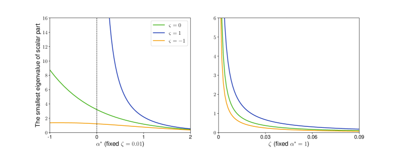
Figure 1: The smallest eigenvalue of the dimensionless coefficient matrix for the scalar part. The left plot depicts the smallest eigenvalue as a function of $\alpha^{\ast}=\alpha+\zeta$ at fixed $\zeta=\beta mc^{2}=0.01$. The right plot depicts the smallest eigenvalue as a function of $\zeta$ at fixed $\alpha^{\ast}=1$. The curve with $\varsigma=1$ in the left plot does not cross the vertical line at $\alpha^{\ast}=0$ because the chemical potential $\mu$ of relativistic Bose gas is not greater than $mc^{2}$.

For the scalar part $\{n^{(1)},\epsilon^{(1)},\Pi^{(1)}\}$ (which corresponds to the upper-left block of the matrix in eq.(64)), it is too difficult to calculate the eigenvalues analytically. However, based on numerical calculations, no eigenvalue less than zero is found. We plot the dimensionless coefficient matrix’s smallest eigenvalue for the scalar part, see Figure 1.

6 Conclusions and remarks

In this work, we have iteratively solved the relativistic Boltzmann equation under the relaxation time approximation in generic stationary spacetime, calculated the first order hydrodynamic variables using the first order solution, and analyzed the first order kinetic coefficients. Moreover, given the important role of Onsager reciprocal relation in conventional non-equilibrium statistical physics [30, 31], we further analyzed these kinetic coefficients. Our calculations show that, up to the first order of the relaxation time the kinetic coefficients satisfy a more generalized Onsager reciprocal relation in the relativistic context, and lead to a non-negative entropy production up to the first order in relaxation time.

A point need to be clarified is that the kinetic coefficients $\{\nu_{i},\sigma_{i},\rho_{i},\kappa_{i},\pi_{i}\}$ are different from the transport coefficients $\{\kappa,\xi\}$. The kinetic coefficients are only relevant to the microscopic theory and not to the choice of hydrodynamic frame, while the definition of transport coefficients depends on the particular hydrodynamic frame. By imposing constraints on the variables $\{\alpha,\beta,U^{\mu}\}$, it is possible to restrict our results to some fixed hydrodynamic frame. In the spirit of BDNK theory [32, 33], a causal, stable, and locally well-posed first order relativistic fluid can be obtained in some particular hydrodynamic frame.

For relativistic systems, the choice of observer can greatly affect the phenomena. Therefore, a question that deserves further consideration is the effect of the choice of observer on the constitutive relations. In addition, at the first order in relaxation time, all the kinetic coefficients are scalars. At the second order of the relaxation time, the kinetic coefficients will be tensors, which lead to more abundant phenomena. We hope to investigate these questions in later study.

Appendix A Calculation of particle flow and energy momentum tensor

We work in orthonormal basis $\{(e_{\hat{a}})^{\mu}\}$ obeying $\eta_{\hat{a}\hat{b}}=g_{\mu\nu}(e_{\hat{a}})^{\mu}(e_{\hat{b}})^{\nu}$. Without loss of generality, we require that $U^{\mu}=c(e_{\hat{0}})^{\mu}$, which implies that the induced metric can be expressed as $\Delta^{\mu\nu}=\delta^{\hat{i}\hat{j}}(e_{\hat{i}})^{\mu}(e_{\hat{j}})^{\nu}$.

For massive particles, the momentum $p^{\hat{a}}=p^{\mu}(e^{\hat{a}})_{\mu}$ can be parameterized by mass shell conditions

$$p^{\hat{a}}=mc(\cosh\vartheta,n^{\hat{i}}\sinh\vartheta),$$ (67)

where $n^{\hat{i}}\in S^{d-1}$ is a spacelike unit vector. Then the momentum space volume element be represented as

$$\boldsymbol{\varpi}=\frac{(\mathrm{d}p)^{d}}{|p_{\hat{0}}|}=\frac{|\boldsymbol{p}|^{d-1}\mathrm{d}|\boldsymbol{p}|\mathrm{d}\Omega_{d-1}}{p^{\hat{0}}}=(mc\sinh\vartheta)^{d-1}\mathrm{d}\vartheta\mathrm{d}\Omega_{d-1},$$ (68)

where $\mathrm{d}\Omega_{d-1}$ is the volume element of the $(d-1)$-dimensional unit sphere $S^{d-1}$. In this way, the integration in the momentum space can be decomposed into integration over $\vartheta\in(0,\infty)$ and integration over the unit sphere $S^{d-1}$.

Here we list some useful integration formulae,

$$\int\mathrm{d}\Omega_{d-1} =\mathcal{A}_{d-1},$$ (69)

$$\int n^{\hat{i}}n^{\hat{j}}\mathrm{d}\Omega_{d-1} =\frac{1}{d}\mathcal{A}_{d-1}\delta^{\hat{i}\hat{j}},$$ (70)

$$\int n^{\hat{i}}n^{\hat{j}}n^{\hat{k}}n^{\hat{l}}\mathrm{d}\Omega_{d-1} =\frac{3}{(d+2)d}\mathcal{A}_{d-1}\delta^{(\hat{i}\hat{j}}\delta^{\hat{k}\hat{l})},$$ (71)

$$\int n^{\hat{i}}\mathrm{d}\Omega_{d-1}=\int n^{\hat{i}}n^{\hat{j}}n^{\hat{k}}\mathrm{d}\Omega_{d-1}=0.$$ (72)

Using eqs.(67)-(72), we can further calculate

$$\int\boldsymbol{\varpi}p^{\mu}f^{(0)}= ~{}\frac{\mathfrak{g}}{h^{d}}\mathcal{A}_{d-1}(mc)^{d}J_{d-1,1}\frac{1}{c}U^{\mu},$$ (73)

$$\int\boldsymbol{\varpi}p^{\mu}p^{\nu}f^{(0)}= ~{}\frac{\mathfrak{g}}{h^{d}}\mathcal{A}_{d-1}(mc)^{d+1}\left(J_{d-1,2}\frac{1}{c^{2}}U^{\mu}U^{\nu}+\frac{1}{d}J_{d+1,0}\Delta^{\mu\nu}\right),$$ (74)

$$\int\boldsymbol{\varpi}\frac{1}{p^{\hat{0}}}p^{\mu}p^{\nu}f^{(0)}= ~{}\frac{\mathfrak{g}}{h^{d}}\mathcal{A}_{d-1}(mc)^{d}\left(J_{d-1,1}\frac{1}{c^{2}}U^{\mu}U^{\nu}+\frac{1}{d}J_{d+1,-1}\Delta^{\mu\nu}\right),$$ (75)

$$\int\boldsymbol{\varpi}\frac{1}{p^{\hat{0}}}p^{\mu}p^{\nu}p^{\sigma}f^{(0)}= ~{}\frac{\mathfrak{g}}{h^{d}}\mathcal{A}_{d-1}(mc)^{d+1}\left(J_{d-1,2}\frac{1}{c^{3}}U^{\mu}U^{\nu}U^{\sigma}+\frac{3}{d}J_{d+1,0}\frac{1}{c}U^{(\mu}\Delta^{\nu\sigma)}\right),$$ (76)

$$\int\boldsymbol{\varpi}\frac{1}{p^{\hat{0}}}p^{\mu}p^{\nu}p^{\sigma}p^{\rho}f^{(0)}= ~{}\frac{\mathfrak{g}}{h^{d}}\mathcal{A}_{d-1}(mc)^{d+2}\biggl{(}J_{d-1,3}\frac{1}{c^{4}}U^{\mu}U^{\nu}U^{\sigma}U^{\rho}$$

$$~{}+\frac{6}{d}J_{d+1,1}\frac{1}{c^{2}}U^{(\mu}U^{\nu}\Delta^{\sigma\rho)}+\frac{3}{(d+2)d}J_{d+3,-1}\Delta^{(\mu\nu}\Delta^{\sigma\rho)}\biggl{)}.$$ (77)

The following calculations are then straightforward,

$$N^{(1)\mu}= ~{}c\int\boldsymbol{\varpi}p^{\mu}f^{(1)}$$

$$= -c^{3}\tau\int\boldsymbol{\varpi}\frac{1}{\varepsilon}p^{\mu}(-p^{\nu}p^{\sigma}\nabla_{\nu}\mathcal{B}_{\sigma}+p^{\nu}\nabla_{\nu}\alpha)\frac{\partial f^{(0)}}{\partial\alpha}$$

$$= -c^{2}\tau\left(-\nabla_{\nu}\mathcal{B}_{\sigma}\frac{\partial}{\partial\alpha}\int\boldsymbol{\varpi}\frac{1}{p^{\hat{0}}}p^{\mu}p^{\nu}p^{\sigma}f^{(0)}+\nabla_{\nu}\alpha\frac{\partial}{\partial\alpha}\int\boldsymbol{\varpi}\frac{1}{p^{\hat{0}}}p^{\mu}p^{\nu}f^{(0)}\right)$$

$$= -c^{2}\tau\frac{\mathfrak{g}}{h^{d}}(mc)^{d}\mathcal{A}_{d-1}\biggl{[}\left(\frac{\partial J_{d-1,1}}{\partial\alpha}\frac{1}{c^{2}}U^{\nu}\nabla_{\nu}\alpha-m\frac{\partial J_{d-1,2}}{\partial\alpha}\frac{1}{c^{2}}U^{\nu}U^{\sigma}\nabla_{\nu}\mathcal{B}_{\sigma}-m\frac{1}{d}\frac{\partial J_{d+1,0}}{\partial\alpha}\Delta^{\nu\sigma}\nabla_{\nu}\mathcal{B}_{\sigma}\right)U^{\mu}$$

$$+\frac{1}{d}\left(-2m\frac{\partial J_{d+1,0}}{\partial\alpha}U^{\sigma}\nabla_{(\sigma}\mathcal{B}_{\nu)}+\frac{\partial J_{d+1,-1}}{\partial\alpha}\nabla_{\nu}\alpha\right)\Delta^{\mu\nu}\biggl{]}$$

$$= -\tau\frac{\mathfrak{g}}{h^{d}}(mc)^{d}\mathcal{A}_{d-1}\biggl{[}\left(\frac{\partial J_{d-1,1}}{\partial\alpha}U^{\nu}\nabla_{\nu}\alpha+mc^{2}\frac{\partial J_{d-1,2}}{\partial\alpha}U^{\nu}\nabla_{\nu}\beta-mc^{2}\frac{1}{d}\frac{\partial J_{d+1,0}}{\partial\alpha}\beta\nabla_{\nu}U^{\nu}\right)U^{\mu}$$

$$+\frac{c^{2}}{d}\left(\frac{\partial J_{d+1,-1}}{\partial\alpha}\nabla_{\nu}\alpha+mc^{2}\frac{\partial J_{d+1,0}}{\partial\alpha}\left(\nabla_{\nu}\beta-\frac{1}{c^{2}}\beta U^{\rho}\nabla_{\rho}U_{\nu}\right)\right)\Delta^{\mu\nu}\biggl{]},$$ (78)

$$T^{(1)\mu\nu}= ~{}c\int\boldsymbol{\varpi}p^{\mu}p^{\nu}f^{(1)}$$

$$= -c^{3}\tau\int\boldsymbol{\varpi}\frac{1}{\varepsilon}p^{\mu}p^{\nu}(-p^{\rho}p^{\sigma}\nabla_{\rho}\mathcal{B}_{\sigma}+p^{\sigma}\nabla_{\sigma}\alpha)\frac{\partial f^{(0)}}{\partial\alpha}$$

$$= -c^{2}\tau\left(-\nabla_{\rho}\mathcal{B}_{\sigma}\frac{\partial}{\partial\alpha}\int\boldsymbol{\varpi}\frac{1}{p^{\hat{0}}}p^{\mu}p^{\nu}p^{\rho}p^{\sigma}f^{(0)}+\nabla_{\sigma}\alpha\frac{\partial}{\partial\alpha}\int\boldsymbol{\varpi}\frac{1}{p^{\hat{0}}}p^{\mu}p^{\nu}p^{\sigma}f^{(0)}\right)$$

$$= -c\tau\frac{\mathfrak{g}}{h^{d}}\mathcal{A}_{d-1}(mc)^{d+1}\biggl{[}\frac{1}{c^{2}}\left(-mc^{2}\frac{\partial J_{d-1,3}}{\partial\alpha}\frac{1}{c^{2}}U^{\sigma}U^{\rho}\nabla_{\rho}\mathcal{B}_{\sigma}-mc^{2}\frac{1}{d}\frac{\partial J_{d+1,1}}{\partial\alpha}\nabla_{\rho}\mathcal{B}_{\sigma}\Delta^{\sigma\rho}+\frac{\partial J_{d-1,2}}{\partial\alpha}U^{\sigma}\nabla_{\sigma}\alpha\right)U^{\mu}U^{\nu}$$

$$+\frac{1}{d}\left(-2mc^{2}\frac{\partial J_{d+1,1}}{\partial\alpha}\frac{1}{c^{2}}U^{\sigma}\nabla_{(\rho}\mathcal{B}_{\sigma)}+\frac{\partial J_{d+1,0}}{\partial\alpha}\nabla_{\rho}\alpha\right)2U^{(\mu}\Delta^{\nu)\rho}$$

$$+\frac{1}{d}(-mc^{2}\frac{\partial J_{d+1,1}}{\partial\alpha}\frac{1}{c^{2}}\nabla_{\rho}\mathcal{B}_{\sigma}U^{\sigma}U^{\rho}-mc^{2}\frac{1}{d}\frac{\partial J_{d+3,-1}}{\partial\alpha}\nabla_{\rho}\mathcal{B}_{\sigma}\Delta^{\sigma\rho}+\frac{\partial J_{d+1,0}}{\partial\alpha}U^{\sigma}\nabla_{\sigma}\alpha)\Delta^{\mu\nu}$$

$$-mc^{2}\frac{2}{(d+2)d}\frac{\partial J_{d+3,-1}}{\partial\alpha}\left(\nabla_{(\rho}\mathcal{B}_{\sigma)}\Delta^{\mu\sigma}\Delta^{\nu\rho}-\frac{1}{d}\nabla_{\rho}\mathcal{B}_{\sigma}\Delta^{\sigma\rho}\Delta^{\mu\nu}\right)\biggl{]}$$

$$= -c\tau\frac{\mathfrak{g}}{h^{d}}\mathcal{A}_{d-1}(mc)^{d+1}\biggl{[}\frac{1}{c^{2}}\left(\frac{\partial J_{d-1,2}}{\partial\alpha}U^{\sigma}\nabla_{\sigma}\alpha+mc^{2}\frac{\partial J_{d-1,3}}{\partial\alpha}U^{\sigma}\nabla_{\sigma}\beta-mc^{2}\frac{1}{d}\frac{\partial J_{d+1,1}}{\partial\alpha}\beta\nabla_{\rho}U^{\rho}\right)U^{\mu}U^{\nu}$$

$$+\frac{1}{d}\left(\frac{\partial J_{d+1,0}}{\partial\alpha}\nabla_{\rho}\alpha+mc^{2}\frac{\partial J_{d+1,1}}{\partial\alpha}\left(\nabla_{\rho}\beta-\frac{1}{c^{2}}\beta U^{\rho}\nabla_{\rho}U_{\sigma}\right)\right)(\Delta^{\rho\nu}U^{\mu}+\Delta^{\rho\mu}U^{\nu})$$

$$+\frac{1}{d}\left(\frac{\partial J_{d+1,0}}{\partial\alpha}U^{\rho}\nabla_{\rho}\alpha+mc^{2}\frac{\partial J_{d+1,1}}{\partial\alpha}U^{\rho}\nabla_{\rho}\beta-mc^{2}\frac{1}{d}\frac{\partial J_{d+3,-1}}{\partial\alpha}\beta\nabla_{\rho}U^{\rho}\right)\Delta^{\mu\nu}$$

$$-mc^{2}\frac{2}{(d+2)d}\frac{\partial J_{d+3,-1}}{\partial\alpha}\beta\left(\Delta^{\rho\mu}\Delta^{\sigma\nu}\nabla_{(\rho}U_{\sigma)}-\frac{1}{d}\nabla_{\rho}U^{\rho}\Delta^{\mu\nu}\right)\biggl{]}.$$ (79)

Data Availability Statement

This work is purely theoretical and contains only analytic analysis. Hence there is no associated numeric data.

Declaration of competing interest

The authors declare no competing interest.

References

[1]
Z. Banach and S. Piekarski, “Perturbation theory based on the Einstein–Boltzmann system. I. Illustration of the theory for a Robertson–Walker geometry,” J. Math. Phys.35 no. 9, (1994) 4809–4831.
[3]
G. Rein, “Stability and instability results for equilibria of a (relativistic) self-gravitating collisionless gas – A review,” [arXiv:2305.02098 [gr-qc]].
[8]
G. V. Vereshchagin and A. G. Aksenov, Relativistic kinetic theory: with applications in astrophysics and cosmology.
Cambridge University Press, 2017.
[21]
X. Hao, S. Liu, and L. Zhao, “Gravito-thermal transports, Onsager reciprocal relation and gravitational Wiedemann-Franz law,” [arXiv:2306.04545 [cond-mat.stat-mech]].
[32]
F. S. Bemfica, M. M. Disconzi, C. Rodriguez, and Y. Shao, “Local well-posedness in Sobolev spaces for first-order conformal causal relativistic viscous hydrodynamics,” [arXiv:1911.02504 [math.AP]].