Non-equilibrium statistical mechanics of the turbulent energy cascade:
irreversibility and response functions

Abstract

The statistical properties of turbulent flows are fundamentally different from those of systems at equilibrium due to the presence of an energy flux from the scales of injection to those where energy is dissipated by the viscous forces: a scenario dubbed “direct energy cascade”. From a statistical mechanics point of view, the cascade picture prevents the existence of detailed balance, which holds at equilibrium, e.g. in the inviscid and unforced case. Here, we aim at characterizing the non-equilibrium properties of turbulent cascades in a shell model of turbulence by studying an asymmetric time-correlation function and the relaxation behavior of an energy perturbation, measured at scales smaller or larger than the perturbed one. We shall contrast the behavior of these two observables in both non-equilibrium (forced and dissipated) and equilibrium (inviscid and unforced) cases. Finally, we shall show that equilibrium and non-equilibrium physics coexist in the same system, namely at scales larger and smaller, respectively, of the forcing scale.

I Introduction

Understanding non-equilibrium systems is one of the most challenging open problem of modern statistical mechanics [1, 2]. A key aspect of non equilibrium phenomena is the presence of currents induced by some external constraints, which entail the breaking of detailed balance and, consequently, of the time-reversal symmetry, or, equivalently, imply the positivity of entropy production [3, 4, 5]. Measuring entropy production is not an easy task as it requires to measure the log-ratio between the probability of a long trajectory of the system and that of its time reversed [6]. This is feasible in relatively simple Markov models but it is hard in general non-equilibrium systems. However, non-equilibrium properties can be inferred by other means: suitable asymmetric time correlation functions can be constructed to unmask the breaking of time reversal symmetry providing a proxy for the departure from equilibrium [7, 8, 9]. Looking at the time evolution of response functions, which describe how some system variables relax to their statistically steady state after a perturbation on the same or different degrees of freedom, can reveal aspects of the asymmetries between degrees of freedom induced by the presence of currents [10, 11, 12].

Fluid flows maintained by an external supply of kinetic energy, acting at large scales, which is dissipated into heat at small scales by viscous forces are characterized by a turbulent-state which is an important example of non-equilibrium statistically steady state [13, 14, 15]. In such a turbulent-state, a current of energy flows from the large to the small scales thanks to the nonlinearity of the Navier-Stokes equation (NSE), with a constant (on average) flux across the scales – after Richardson this is dubbed the direct energy cascade scenario [14]. Typically the energy cascade is studied in terms of single time statistical objects, e.g. the third order moment of the velocity differences between points at distance $r$ is directly linked to the energy flux via the celebrated $4/5$ law [14], which is one of the few exact results that can be obtained on the turbulent-state and entails a spatial asymmetry in the statistics of the fluctuations of the velocity field. Much fewer studies attempted a direct study of the energy cascade, and the consequential asymmetries, with reference to the time evolution of the flow [8, 9].

In this paper, we aim at studying the temporal properties of the turbulent energy cascade in terms of two statistical tools: asymmetric time correlations and response functions. We apply these tools to shell models [16, 17, 18] that are relatively (with respect to NSE) low dimensional dynamical systems that phenomenologically (and to some extent quantitatively) reproduce the main features of the turbulent energy cascade. Such models are constructed without a spatial structure using a discrete number of Fourier shells with an associated complex variable, representing the velocity fluctuation at that scale (inverse of wavenumber). This simplified structure makes, in comparison to real fluid flows, the study of the temporal properties easier while maintaining the main phenomenological features of the problem [19, 20, 21]. In particular, we consider the so-called Sabra shell model [22] and study suitable asymmetric time correlations of the energy at a given shell and response functions to energy perturbations. Specifically, concerning the latter, we test non-diagonal responses, i.e. we study how a perturbation of the energy at a given shell alters the relaxation of the energy of neighboring shells both in and against the direction of the energy flux. Previous studies in the shell model [23, 24] focused on diagonal response functions considering perturbations of the shell velocity. While such a procedure is interesting with respect to the fluctuation dissipation relations [25, 11, 26], it is not able to reveal the asymmetries induced by the cascade, which are, instead, clearly detected when perturbing the shell energy and looking at non-diagonal response functions.

At first we compare the behavior of the asymmetric time correlations and response functions either when the system is forced and dissipated or unforced and inviscid. In the latter case, unlike the former, an equilibrium state establishes similarly to the well known absolute equilibrium of the truncated Euler equations [27, 13], which were numerically studied by looking either at the transient stages leading to the equilibrium state [28] or at the spatio-temporal decorrelation of two copies of the system [29]. The inviscid shell model represents a toy model version of the truncated Euler equations. The asymmetric time correlations of the energy vanish for the inviscid (equilibrium) shell model while are clearly different from zero in the forced and dissipated (non-equilibrium) shell model, quantifying the breaking of time reversibility. In particular, we show that it is enough to look at the short time behavior of such correlations which is associated to the third order moment of the shell energy rate of change, similarly to what observed in Ref. [9] for tracer dynamics. Similarly, clear asymmetries in the relaxation of energy at wavenumbers smaller or larger than the perturbed shell distinguish the non-equilibrium and equilibrium cases and the direction of the cascade in the former case. Then, we apply these tools to the case in which the shell model is forced at intermediate scales. At scales smaller than the forced one the usual energy cascade is expected while, as we will show, at larger scales the behavior of correlations and responses is compatible with an equilibrium state as conjectured [14] and to some extent shown also in direct numerical simulations of NSE [30, 31] and experiments [32], although this was recently challenged [33, 34].

The paper is organized as follows. In Sec. II we introduce the shell model for turbulent energy cascade and make a resume of its main properties. Section III presents the main tools used to probe the non-equilibrium properties of the energy cascade, namely the asymmetric correlation functions and the non-diagonal energy response functions. In Sec. IV we present the results, in particular: first we contrast the behavior of the asymmetric correlations of the shell energy in the shell model forced at large scales with those of the inviscid and unforced shell model; then we explore the non-diagonal energy response functions in the same settings; finally we consider the forced shell model and explore the behavior of the two quantities at scales larger and smaller than the forcing scale in order to ascertain the equilibrium or non-equilibrium character of the former. Section V is devoted to conclusions and offers a perspective on future investigations. Several Appendices complement the main text: App. A provides some details on the simulations including a table with the parameters; App. B discusses some subtleties related to the computation of the asymmetric correlation functions; App. C complements the study of the inviscid unforced shell model; finally, App. D provides a derivation for the small time behavior of the energy response functions.

II Model

Shell models are finite-dimensional dynamical systems designed to reproduce the phenomenology of the turbulent energy cascade [16, 17, 18]. The basic idea is to consider a discrete set of wavenumber $k_{n}\!=\!k_{0}2^{n-1}$, the shells with index $n\!=\!1,\ldots,N$. A single complex variable, $u_{n}$, is used to represent the velocity fluctuations at scale $k_{n}$. The velocity variables $\{u_{n}\}_{n=1}^{N}$ evolve with a set of equations formally analogous to the Navier-Stokes equation in Fourier space:

$$\dot{u}_{n}\!=ik_{n}Q[u,u]\!-\!\nu k_{n}^{2}u_{n}\!+\!f_{n}\,,$$ (1)

where $\nu$ is the viscosity and $f_{n}$ the forcing. The quadratic term $Q(u,u)$ is built to ensure that in the unforced and inviscid limit ($f_{n}\!=\!\nu\!=\!0$), as for the three-dimensional Euler equation, the dynamics preserves both energy $E$ and helicity $H$, that, for the shell model, read

$$E = \sum_{n=1}^{N}e_{n}\,,$$ (2)

$$H = \sum_{n=1}^{N}(-1)^{n}k_{n}e_{n}\,,$$ (3)

where $e_{n}=|u_{n}|^{2}/2$ is the energy of shell $n$. Yet there is some freedom in choosing the quadratic term $Q(u,u)$; here, we consider the Sabra model [22], for which

$$Q(u,u)=2u_{n+2}u_{n+1}^{*}\!-\!\tfrac{1}{2}u_{n+1}u_{n-1}^{*}\!+\!\tfrac{1}{4}u_{n-1}u_{n-2}\,,$$ (4)

where ^∗ denotes complex conjugation, with boundary conditions $u_{-1}\!=\!u_{0}\!=u_{N+1}\!=\!u_{N+2}\!=\!0$. The choice to restrict the quadratic interactions to neighboring shells is justified by the idea that the energy cascade is local in scale [13], i.e. the energy transfer is mainly due to the interaction with close-by scales. As demonstrated in many studies (see, e.g., Refs. [16, 17, 18]), shell models, including the Sabra [22], display the same phenomenology of the turbulent energy cascade.

The forcing $f_{n}$, usually localized around some scale $1/k_{n_{f}}$ ($f_{n}\neq 0$ for $n\sim n_{f}$), injects energy at a rate $\epsilon=\sum_{n}\langle\Re\{f_{n}u_{n}^{*}\}\rangle$, where $\langle\cdot\rangle$ denotes time averages and $\Re\{\cdot\}$ the real part. The nonlinear term transfers the energy at smaller scales, on average, with a constant flux equal to $\epsilon$. And, at large enough wavenumber, the viscous term becomes important and removes the energy at a rate $\nu\sum_{n}k_{n}^{2}\langle|u_{n}|^{2}\rangle=\nu\Omega=\epsilon$ ($\Omega$ being the enstrophy). In this way, a non-equilibrium steady state is established, which can be described by the energy balance equation

$$\dot{E}_{M}=-\Pi_{M}-\nu\Omega_{M}+\sum_{m=1}^{M}\langle\Re\{f_{m}u_{m}^{*}\}\rangle\ ,$$ (5)

where $E_{M}=\sum_{m=1}^{M}\langle e_{m}\rangle$ and $\Omega_{M}=\sum_{m=1}^{M}k_{m}^{2}\langle e_{m}\rangle$ ($M\leq N$) are the average energy and enstrophy up to wavenumber $M$, respectively; while

$$\Pi_{M}\!\!=\!\Delta_{M+1}\!+\!\tfrac{1}{2}\Delta_{M}\,,\quad\Delta_{m}\!\!=\!k_{m}\Im\{u_{m+1}u^{*}_{m}u^{*}_{m-1}\}\,,$$ (6)

$\Im\{\cdot\}$ denoting the imaginary part, is the energy flux transferred to shells $>M$ (viz. minus the rate of energy loss from shells $\leq M$) due to the nonlinear terms. Notice that $E_{N}=E$ and $\Pi_{N}=0$, since the non-linear term preserves energy, so that when summing over all the shells $\dot{E}=\epsilon-\nu\Omega=0$, i.e. energy is conserved on average. For shells $m$ between the forced one ($n_{f}$) and that where dissipation becomes effective the average energy flux is constant $\Pi_{m}=\epsilon$ (as $\dot{E}_{m}=0$ for each $m$ at stationarity), which is the hallmark of the energy cascade. From $\Pi_{m}=\epsilon$ and (6) one can dimensionally see that $u_{n}\sim(\epsilon k_{n}^{-1})^{1/3}$ which is the Kolmogorov 1941 [14] prediction for the shell model, which allows to estimate the dissipative wavenumber as $k_{n_{d}}\approx(\epsilon/\nu^{3})^{1/4}$.

Remarkably, shell models also reproduce some quantitative aspects of the statistical properties of turbulent flows as, for instance, the anomalous scaling of the velocity structure functions (moments of velocity differences), which can be expressed as $\langle|u_{n}|^{p}\rangle$ and, in the inertial range ($n_{f}<n<n_{d}$), are found to scale as

$$S_{p}(k_{n})=\langle|u_{n}|^{p}\rangle\sim k_{n}^{-\zeta(p)}$$ (7)

with $\zeta(p)$ very close to the exponents measured in turbulent flows, and thus deviating from the Kolmogorov dimensional prediction $p/3$.

In the inviscid and unforced case ($\nu=f_{n}=0$), the system sets on an equilibrium statistically stationary state while evolving on a manifold dictated by the value of the energy and helicity, akin to the one of truncated Euler equations [27, 13] (see also Refs. [28, 29]). Thus, the SABRA model does offer a nice laboratory to contrast the equilibrium and non-equilibrium properties of the Euler and Navier-Stokes equations, which is the aim of this paper.

We will consider the Sabra model forced at large scales and contrast it with the unforced inviscid case and, also, the Sabra model forced at intermediate scales. In the latter case one expect that at scales above the forcing the physics will be akin to that of the inviscid case (i.e. equilibrium) and below the forcing scale characterized by a direct energy cascade (i.e. non-equilibrium) [30, 31, 32, 35].

We conclude this section mentioning that in the rest of the paper we shall present simulations obtained by using a forcing which imposes a fixed energy input $\epsilon=1$. However, we tested that the results remain qualitatively unchanged by using a constant forcing on a single shell. Appendix A provides other details on the numerical implementation and the parameters which have been used.

III Probing the non-equilibrium properties of the turbulent cascade

Let us now present the main statistical mechanics tools we used to characterize the non-equilibrium properties of the energy cascade, namely: asymmetric correlation functions, which allow for detecting irreversibility [7, 8, 9], and response functions [11], which by describing how observables at a given shell $n$ behave after a suitable perturbation is performed at shell $m$ allow for highlighting the asymmetries between shell variables induced by the energy flux.

III.1 Testing the breaking of time-revesal symmetry via asymmetric correlation functions

The hallmark of out-of-equilibrium systems is the breaking of the time-reversal symmetry that, mathematically, stems from the absence of detailed balance with the associated positive entropy production [3, 4, 5]. However, entropy production is a global quantity difficult to measure. Here, to detect temporal asymmetries, we take an alternative route by looking at the behavior of suitable correlation functions. Indeed, as made clear e.g. by Onsager [36], for any choice of observable functions $f$ and $g$ of the system state, at equilibrium one has $\langle f(t)g(0)\rangle=\langle f(0)g(t)\rangle$ due to time reversibility. This result entails that if there exist $f$ and $g$ such that $\langle f(t)g(0)\rangle\neq\langle f(0)g(t)\rangle$ the system is out-of-equilibrium, and the difference $\langle f(t)g(0)\rangle-\langle f(0)g(t)\rangle$ can be taken as a proxy of the distance from equilibrium. The functions $f$ and $g$ could refer to different observables of the system, e.g. different dynamical variables, or if the same observable is used one must consider appropriate functions thereof.

Here, following Refs. [7, 8], after denoting with $x(t)$ a statistically stationary signal representing the temporal evolution of an observable of the system, we will consider asymmetric time-correlation functions of $x$ to detect breaking of time reversal and thus the signature of non-equilibrium. In particular, we consider the function [8]

$$\Psi_{x}(\tau)\equiv\langle x^{2}(t)x(t+\tau)\rangle-\langle x(t)x^{2}(t+\tau)\rangle\,,$$ (8)

which, for a stationary signal, can be equivalently written as

$$\Psi_{x}(\tau)=\tfrac{1}{3}\langle[x(t+\tau)-x(t)]^{3}\rangle\equiv\Phi_{x}(\tau)\ .$$ (9)

This latter expression was used in [9] to reveal the irreversibility of tracers dynamics in turbulence. While mathematically $\Phi_{x}(\tau)=\Psi_{x}(\tau)$, in numerical computation of Eqs. (8) and (9) some differences may appear due to unlike statistical convergence, especially at small time lags. Such differences, as discussed in Appendix B, if not properly considered may lead to spurious results.

In particular, in the case of the shell model, we shall compute the above introduced correlation function using as observable the instantaneous energy at shell $n$, i.e. $x(t)=e_{n}(t)=\frac{1}{2}|u_{n}(t)|^{2}$, and consider different shells. As clear from Eq. (9), this choice is expected to provide also some hints on the energy cascade process as it informs us about how the energy of a shell varies in time. We notice that taking as $x(t)$ the signal of the real or imaginary part of the shell velocity leads to results essentially indistinguishable from equilibrium. This means that it is important to use proper observables.

III.2 Testing asymmetries among the degrees of freedom via non-diagonal response functions

One of the most distinguishing aspects of out-of-equilibrium systems is the presence of currents, e.g. of matter or energy [37]. Besides breaking the time-reversal symmetry, as discussed in the previous section, these currents generate asymmetries in the degrees of freedom of the system. In the specific case of turbulence, energy flows from the injection scale towards smaller scales until it is dissipated at very small ones. Thus there is a wide range of scales, which increases with the Reynolds number [15], interested by such an asymmetry. In other systems the lack of symmetry may lead to spatial inhomogeneity between the degrees of freedom [12].

A powerful statistical mechanics tool to explore such asymmetries is the study of response functions (RFs) [11]. The idea is rather simple, if we consider generic time-dependent observables having $M$ components with $\bm{A}(t)=\{A_{m}(t)\}_{m=1,\dots,M}$ and $\bm{B}(t)=\{B_{n}(t)\}_{n=1,\dots,M}$, and we denote with $\bm{A}^{\prime}(t)$ and $\bm{B}^{\prime}(t)$ their trajectory after a perturbation of one of the components of $\bm{A}$, then the usual definition of (impulsive) response function reads:

$$R_{A_{m},B_{n}}(t)=\frac{\overline{B^{\prime}_{n}(t)-B_{n}(t)}}{A^{\prime}_{m}(0)-A_{m}(0)}\equiv\frac{\overline{\delta B_{n}}(t)}{\delta A_{m}(0)}\ ,$$ (10)

where $\delta[\cdot]$ is the difference between the value in the perturbed system and that in the unperturbed one, while $\overline{[\cdot]}$ denotes the statistical average over many different realizations of the experiment. The above formula measures how much an instantaneous perturbation on $A_{m}$ influences, on average, the variable $B_{n}$ at later times.

In the case of the shell model a natural observable to perturb is the energy at a given shell $e_{m}(t)=\frac{1}{2}|u_{m}(t)|^{2}$ and then to look at the effect of the perturbation on the energies at shells larger (scales smaller) and smaller (scales larger) than $m$. Owing to the energy flux a clear asymmetry between the two directions should be expected, while it should be absent in the equilibrium case, i.e. in the inviscid and unforced limit. To the best of our knowledge previous attempts to measure the response functions in the shell model [23, 38] only considered diagonal responses with respect to infinitesimal perturbations on the shell velocity $u_{m}$ at a given scale. Here, the main novelty is to perturb the energy by a non-infinitesimal amount (somehow similarly to Ref. [39]) and to explore non-diagonal responses, $R_{e_{m},e_{n}}(t)$ ($n\neq m$). In the following, we shall denote such response function as $R_{m,n}(t)$ to ease the notation.

In principle, it is not needed to physically perturb a system in order to study the response functions. In the linear perturbation regime, RFs are linked, via the fluctuation-dissipation relations (FDRs), to suitably defined correlation functions [25, 11, 26]. As an important example, we mention the Green-Kubo formulas [25] which link the response to an external field with correlations computed at equilibrium. FDRs, originally derived for equilibrium Hamiltonian systems, apply also to non-equilibrium systems as any response can be expressed as correlation functions whose functional form depends on the invariant measure of the system [40, 41]. It is worth stressing that there is still a certain confusion in the literature on this aspect. Indeed, FDRs hold under very general assumptions and are only slightly more complicated for dissipative chaotic systems. Such complications, which are independent of the equilibrium or non equilibrium nature of the system, arise due to the singular character of the invariant measure. However, with the addition of a small amount of noise in the dynamical equations (i.e. smoothing the measure) it is still possible to compute RFs via some correlation function [42, 43, 44]. This idea has been exploited, e.g., in the context of the shell model in [38].

In general, for all systems which cannot be directly probed via perturbations (the climate is in this respect an example of utmost importance [45, 46]) it is crucial to exploit FDRs to understand the possible effect of local disturbances. However, in our study we shall directly study the energy RFs, since from a computational point of view exploiting FDRs as in Refs. [42, 43, 44] would anyway require a modification of the equation with the addition of noise and a huge statistics in order to allow for cancellations in the correlation functions [38].

Figure 1: Asymmetric time-correlation functions $\Psi_{e_{n}}(t)$ at varying $n$ as labeled. (a) Turbulent case, shells $n$ in the inertial range. Different functions show a qualitatively similar behavior, and symmetry under time reversal is absent. Statistics: $6\cdot 10^{5}$ samples. (b) Inviscid case, shells $n$ as labeled in the range with energy equipartition. Small fluctuations around zero are compatible with $\Psi_{e_{n}}(t)=0$. Statistics: $5\cdot 10^{5}$ samples.

IV Results

We present now the results obtained with numerical simulations performed on the Sabra shell model, of both inviscid and viscous type. We will highlight the differences between a system at equilibrium (the former) and a system out-of-equilibrium (the latter). We shall first discuss the test of irreversibility (Sec. III.1) and the response-functions (Sec. III.2) for the shell model either forced at large scales (run-LSF) or unforced and inviscid (run-Eq), for the parameters see Table 1 of App. A. Then we shall discuss the shell model forced at intermediate scales (run-ISF), showing that the physics at scales larger than the forcing scale is akin to the inviscid model (equilibrium) while at scales smaller than the forcing is that of the non-equilibrium energy cascade.

IV.1 Irreversibility

As discussed in Sec. III.1 in order to test the irreversibility of the energy cascade we focus on the energy signal $e_{n}(t)=|u_{n}|^{2}/2$ at shell $n$ (by varying $n$). In particular, we measure the asymmetric correlation function $\Psi$ (8) or, equivalently, $\Phi$ (9), which we rewrite as

$$\Psi_{e_{n}}(\tau)=\frac{\langle e_{n}^{2}(t)e_{n}(t+\tau)\rangle-\langle e_{n}(t)e_{n}^{2}(t+\tau)\rangle}{\langle e_{n}^{3}(t)\rangle}=$$

$$= \Phi_{e_{n}}(\tau)=\frac{1}{3}\frac{\langle[e_{n}(t+\tau)-e_{n}(t)]^{3}\rangle}{\langle e_{n}^{3}(t)\rangle}\,,$$ (11)

to simplify the notation we have used the same symbol, even if the two quantities are now made nondimensional. We also recall that the two different expressions should coincide for a stationary signal, but can be numerically different for finite statistics (see App. B).

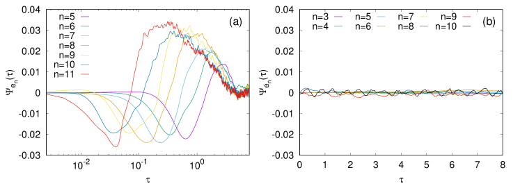
The inviscid and unforced shell model reaches an equilibrium statistically stationary state with no net currents and, thus, detailed balance holds, implying that forward and backward dynamics are indistinguishable. As a consequence we should expect that $\Psi_{e_{n}}(\tau)=\Phi_{e_{n}}(\tau)=0$. Conversely, for the forced and dissipated shell model, owing to the presence of an energy flux from the large to the small scales, the dynamics is irreversible and $\Psi_{e_{n}}(\tau)\neq 0$. Such expectations are well verified as shown in Fig. 1: apart from unavoidable fluctuations, $\Psi_{e_{n}}(\tau)=0$ for the inviscid model (Fig. 1b), while for the forced model is clearly different from zero (Fig. 1a) and, actually, it displays several interesting features.

Figure 2: Same as Fig. 1(a) with time rescaled by (a) $\tau_{n}=k_{n}^{-0.76}$ (see text for a discussion) and (b) $k_{n}^{-0.5}$, where $0.5$ was chosen in such a way to line up the maxima. The vertical dashed lines are drawn to guide the eyes making clearer the line up.

Figure 3: (a) Asymmetric moments $-\mathcal{A}_{q}(k_{n})$ (Eq. (14)) vs the shell number $n=\log_{2}(k_{n}/k_{0})$, for increasing $q=s/3$ with $s=4,\ldots,9$ (from bottom to top). The moments for $q<1$ are positive (not shown) and $\mathcal{A}_{1}(k_{n})=0$ by stationarity. The lowest and highest shells are omitted. (b) Symmetric moments $S_{q}(k_{n})$ (Eq. (13)) (empty symbols) and asymmetric ones $-A_{q}(k_{n})$ (filled symbols) rescaled by their value at $n=3$ for three values of $q$, as labeled. The black solid lines display the prediction (15). Inset: the ratio $-A_{q}(k_{n})/S_{q}(k_{n})$, with $q=s/3$ for $s=1,\ldots,9$ from bottom to top. Statistics is over $2.5\cdot 10^{6}$ samples.

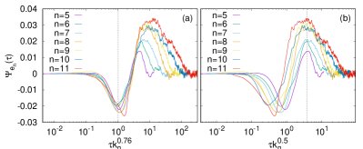
First of all, for small time lags $\Psi_{e_{n}}(\tau)$ is negative while it becomes positive at larger time lags and then it approaches zero at much larger $\tau$’s. This is consistent with the idea that energy decreases on a fast time scale and increases over a longer time scale (notice that by stationarity $\langle e_{n}(t+\tau)\rangle=\langle e(t)\rangle$). This is similar to the flight-crash events described in Ref. [9] but at the level of a single shell. The fact that the energy loss is faster than the energy gain is physically understood from the fact that the time scale of the shell decreases with the scale as $\tau_{n}\sim(u_{n}k_{n})^{-1}\sim k_{n}^{-2/3}$ (where we used Kolmogorov scaling). Therefore, it takes longer to receive energy from larger and slower scales (smaller $n$) than to transfer it to smaller scales (larger $n$). However, as already clear from Fig. 1a, in the temporal behavior of $\Psi_{e_{n}}(\tau)$ several time-scales are at play. Indeed one can see that the short time minima depends on the shell index $n$ while the large-time decay of the curves is essentially independent of $n$, as the curves reach zero at about the same time. The presence of many time scales is even clearer by looking at Fig. 2, showing that different rescaling of the time lags depending on the scale as $k_{n}^{\beta}$ are needed to make either the minima ($\beta\approx 0.76$, Fig. 2a) or the maxima ($\beta\approx 0.5$, Fig. 2b) line up. While we have no clear understanding of the latter exponent, the first one can be understood as follows.

As discussed in the next section and Appendix B, at short times it should hold

$$\Psi_{e_{n}}(\tau)=\Phi_{e_{n}}(\tau)\approx\frac{\langle\dot{e_{n}}^{3}\rangle}{\langle e_{n}^{3}\rangle}\tau^{3}\,.$$ (12)

Equations (7) and (15) (see next section) imply that ${\langle\dot{e_{n}}^{3}\rangle}/{\langle e_{n}^{3}\rangle}\sim k_{n}^{3-\zeta(9)+\zeta(6)}$. From our simulations we get $\zeta(6)\approx 1.70(2)$ and $\zeta(9)\approx 2.43(6)$. If we now re-scale $\tau$ in Eq. (12) with $\tau_{n}\sim k_{n}^{-\beta}$ by requiring that the expression does not depend on $n$ we have $\beta=(3-\zeta(9)+\zeta(6))/3\approx 0.76(3)$, which is well compatible with Fig. 2a. We also notice that $\Psi_{e_{n}}$ is the difference of two disconnected, single scale and multi-time correlation functions that, as thoroughly discussed in Ref. [20], should involve a whole hierarchy of fluctuating eddy-turnover times from the shortest up to the largest. In Ref. [20] it was discussed the general framework of multi-time and multiscale correlation functions, similarly to $\Psi_{e_{n}}$: one can define suitable correlations involving energy at different shells and different times, which besides providing information on the irreversibility can also further characterize the physics of the energy cascade. However, this goes beyond the aim of this work and we leave it for possible future studies.

Figure 4: Non-diagonal energy RFs $R_{m,n}$, with error bars, measured at the neighboring shells of the perturbed one. (a) Turbulent Sabra model. Initial energy perturbation: $\delta_{m=11}\simeq 9.93\cdot 10^{-3}$. (b) Inviscid Sabra model. The initial transient is plotted with logarithmic time axis up to the red vertical line, the later stages with a linear axis. Another RF has been added (green plot), with more distance between $m$ and $n$, in order to show the common asymptotic value. The dot-dashed line shows $R^{(\infty)}_{eq}$ which is the value that would be reached if perfect energy equipartition occurs, the dashed line shows $R^{(\infty)}_{corr}$ which is the asymptotic value taking into account the boundary corrections (see App. C and main text). Initial perturbation $\delta_{m=6}=\delta_{m=7}\simeq 1.79\cdot 10^{-3}$. The insets of both figures are enlargements of the initial-time range, showing respectively a non-zero and a zero first derivative at $t=0$. In all figures statistics is over $5\cdot 10^{5}$ realizations.

IV.1.1 Power fluctuations

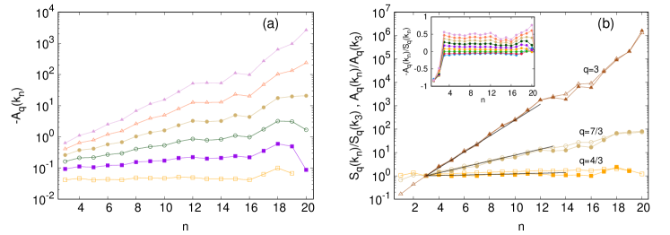
The negativity of $\Psi_{e_{n}}(\tau)$ for small $\tau$ can be further scrutinized by studying directly the $\tau\to 0$ limit. Indeed by expanding Eq. (11) for small $\tau$ (see Appendix B, also for a discussion on the subtle numerical aspects related to the short time behavior of $\Psi$ and $\Phi$) it is easy to realize that the initial negativity means that $\langle\dot{e}_{n}^{3}\rangle<0$, while we know by stationarity that $\langle\dot{e}_{n}\rangle=0$: this means that the statistics of $\dot{e}_{n}$ is negatively skewed, which confirms the fact that it is more probable to lose than to gain energy on the short time. This observation was originally made in Ref. [9] in the context of irreversibility of Lagrangian trajectories in turbulence, and further analyzed in [21] in both direct numerical simulations and in shell model version of Lagrangian motion. In particular, in Ref. [21] it was introduced a set of symmetric and asymmetric moments to probe the asymmetry of the distribution. Here, following [21], we consider the moments:

$$\mathcal{S}_{q}(k_{n}) = \langle|\dot{e}_{n}|^{q}\rangle/\epsilon^{q}$$ (13)

$$\mathcal{A}_{q}(k_{n}) = \langle\dot{e}_{n}|\dot{e_{n}}|^{q-1}\rangle/\epsilon^{q}$$ (14)

where the normalization by $\epsilon^{q}$ is only to make the quantities dimensionless. Numerical simulations show that $\mathcal{A}_{q}(k_{n})>0$ for $q<1$ and $<0$ for $q>1$, for $q=1$ is zero by stationarity. Moreover, as shown in Fig. 3a, the asymmetric moments display a power law behavior, $-A_{q}(n)\sim k_{n}^{\alpha(q)}$. To rationalize the exponents $\alpha(q)$ we can use dimensional analysis in the spirit of the multifractal model [14]. Noticing that $\dot{e}_{n}$ is energy divided by time, we can assume that for each shell one has to use its own characteristic eddy turnover time, that dimensionally can be estimated as $\tau_{n}\sim 1/(|u_{n}|k_{n})$, so that

$$\langle\dot{e}_{n}^{q}\rangle\sim\langle|u_{n}|^{2q}k_{n}^{q}|u_{n}|^{q}\rangle\sim k_{n}^{q}S_{3q}(k_{n})\sim k_{n}^{q-\zeta(3q)}\,,$$ (15)

where we used (7) in the last two steps. It should be noted that this argument is purely dimensional, thus it applies both to the symmetric and asymmetric moments. It is worth stressing that it is not obvious a priori that $S_{q}(k_{n})$ and $-A_{q}(k_{n})$ should scale in the same way nor that the asymmetric moment can be guessed with a dimensional argument, indeed it depends on cancellations which cannot be controlled. However, Fig. 3b shows that $S_{q}(n)$ and $-A_{q}(n)$ possess the same scaling behavior (see also the inset) and agree with the prediction (15).

IV.2 Energy response functions

In order to detect the scale asymmetry between shells, caused by the average energy flux from large to small scales, we study non-diagonal RFs on the shell energies $e_{n}(t)$ (see also Sec. III.2):

$$R_{m,n}(t)=\frac{\overline{\delta e_{n}}(t)}{\delta e_{m}(0)}\ ,$$ (16)

the first index referring to the perturbed shell and the second to the shell one looks at. To fix the initial energy perturbation $\delta e_{m}(0)$ of each experiment we introduce the following perturbation on the velocity at $t=0$:

$$u_{m}=\sqrt{2e_{m}}e^{i\theta_{m}}\quad\longrightarrow\quad u_{m}^{\prime}=\sqrt{2(e_{m}+\delta_{m})}e^{i\theta_{m}}$$ (17)

where $\theta_{m}$ is the phase of $u_{m}$, and $\sqrt{2e_{m}}$ its modulus. The constant $\delta_{m}$ quantifies the magnitude of the initial energy perturbation while keeping the phase of $u_{m}$ fixed, and is such that: $\delta e_{m}(0)=\delta_{m}$. The phases are crucial for the energy transfer [47] that is why we keep them constant. Moreover, we consider a non-infinitesimal perturbation: specifically, we choose $\delta_{m}$ to be a finite fraction of the typical fluctuation of the shell energy, namely its standard deviation:

$$\delta_{m}=f\sigma_{e_{n}}=\frac{f}{2}\sqrt{\langle|u_{n}|^{4}\rangle-\langle|u_{n}|^{2}\rangle^{2}}\ ,$$ (18)

in which $f\simeq 0.2$ was used.

Figure 5: Relative energy deviation (19) at consecutive shells, with fixed perturbed shell $m$, in the turbulent shell model: (a) for shells $n>m=5$, with $\delta_{m=5}\simeq 0.1$; (b) for shells $n<m=14$ and $\delta_{m=14}\simeq 2.74\cdot 10^{-3}$. The insets show the un-rescaled RFs. Statistics is over $5\cdot 10^{5}$ iterations.

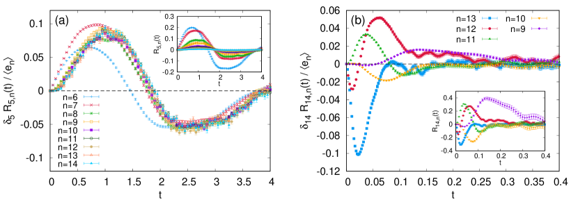
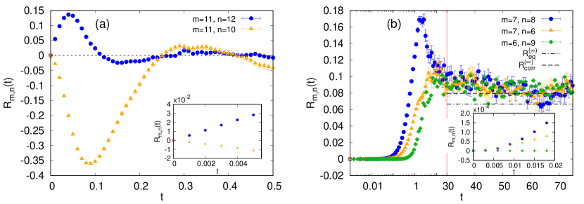
In Fig. 4 we compare the RFs $R_{m,n}$ with $n-m=\pm 1$ in the turbulent (panel a) and inviscid (panel b). The functions in Fig. 4(a) clearly display the asymmetry between degrees of freedom mentioned before: in the turbulent system the opposite sign of the “forward” (towards smaller scales) and “backward” (towards larger scales) RFs reveals the presence of an overall energy current, displacing energy from larger to smaller scales. The different amplitudes and relaxation times relates to the fact that larger scales have larger amplitudes and are slower than the smaller scales. On the other hand, such an asymmetry is clearly lost in the inviscid system, as shown in Fig. 4(b): the RFs are all positive, and after an initial transient they approach a common non-zero asymptotic value. This trend is explained as follows. In the inviscid system energy (but also helicity) is conserved, therefore the energy perturbation brings the system to a larger constant-energy hyper-surface in phase space. Assuming a perfect energy equipartition one can compute the expected long-time value $R_{\text{eq}}^{(\infty)}=1/N$, however as discussed in Appendix C boundary effects prevent perfect equipartition. Taking them into account one can compute a corrected asymptotic value, $R_{\text{corr}}^{(\infty)}$, which fits better with the data as shown in Fig. 4(b)

It is equally interesting to notice that short shell-distance RFs show non-zero initial derivatives in the turbulent case, whereas they are zero in the inviscid system (see the insets of Fig. 4). Briefly, this is due to the presence or absence, respectively, of energy cascades in the system, since these derivatives are related to the order-three correlator describing the energy flux through the shells, as detailed in Appendix D.

Figure 6: Energy spectrum $\langle e_{n}\rangle$ for the Sabra shell model with forcing at intermediate scales. The three regimes of energy equipartition, power-law scaling and viscous damping can be identified. The dashed line corresponds to the scaling $\langle e_{n}\rangle\sim k_{n}^{-\zeta(2)}$, with $\zeta(2)\approx 0.74(4)$. Inset: average flux $\Pi_{n}$ (6) out of shell $n$. There is a clear transition from zero to positive outward flux. The small arrows in both figures indicate the forced shells. Statistics: $10^{6}$ samples.

Figure 7: Asymmetric time correlation functions (11) measured at shells larger than the forced ones, as in label. Inset: the same correlations, measured at shells below forcing, $n$ ranging from 5 (lighter) to 11 (darker). Statistics: $5\cdot 10^{5}$ samples.

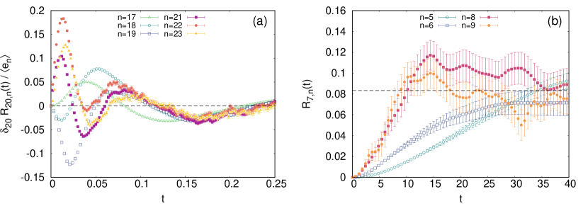
To offer a more complete investigation of the turbulent cascade we also studied the response of shells further-apart from the perturbed one. Owing to the fact that the energy spectrum decays as a power law, in the main panel of Fig 5(a) we show the relative energy deviation,

$$\frac{\delta_{m}}{\langle e_{n}\rangle}R_{m,n}=\frac{\overline{\delta e_{n}}(t)}{\langle e_{n}\rangle}\ ,$$ (19)

for $n>m$. The advantage of the relative deviation (19) is that it allows for normalizing the amplitude of the response making possible the comparison of the response of shells at different distances from the perturbed one. Figure 5(b) shows the same for shells smaller than the perturbed one. The insets represent the usual (non-normalized) RFs. The energy deviations in the forward direction collapse nicely onto the same curve, apart from the functions with $n-m=1,2$. These two are the only functions whose index $n$ is in the same wave-number triad of shell $m$, so a difference with the other functions can be expected. On the other hand, the energy deviations in the backward direction lack any kind of similarity between themselves, and their short-time value, before the relaxation, can be indeed positive (energy gain) or negative (energy loss) for different values of $n-m$. Unlike the forward functions, the backward ones show smaller amplitudes as the distance from the perturbed shell grows. Overall, a correct interpretation of the latter RFs requires a better understanding of how the different time-scales involved, from the slowest to the one with shell index $\text{max}\{m,n\}$, contribute to the energy deviation, in the same way as assumed for multi-time multi-scale correlation functions [20]. And this is out of the scope of the present work.

Figure 8: Energy response functions in the Sabra model with forcing at intermediate scales: (a) RFs normalized as in (19) when perturbing shell $m=20$ in the inertial range. Both the forward ($n>m$) and the backward ($n<m$) functions are qualitatively similar to those of Fig. 5a and b, respectively. (b) $R_{m,n}$ for $m=7$ in the middle of the equiparted part of the spectrum, above the forced shell. The RFs approach a common asymptotic value as in Fig. 4(b). The dashed line is estimated as $R_{eq}^{(\infty)}=1/N^{*}$, where $N^{*}$ is the number of shells for which energy equipartition holds. In both cases statistics is over $2\cdot 10^{5}$ realizations.

IV.3 Equilibrium/non-equilibrium at scales larger/smaller than the forcing scale

So far we have discussed either the case of the inviscid, unforced shell model or the forced shell model, showing how asymmetric energy correlations or the energy RFs can reveal the asymmetries and breaking of time reversal induced by the energy flux from the scale of forcing to the smaller scales. It is now natural to wonder what does happen at scales larger than the forcing scale. Since such scales are not directly influenced neither by the forcing nor by the viscous damping and owing to the direct cascade, it has been conjectured that the physics of these large scales should be akin to the equilibrium one [14]. Numerical [30, 48, 35, 31] and experimental [32] studies indeed seem to confirm that many aspects of the scales above the injection scale are well captured by absolute equilibrium theory [27]. Two recent studies [33, 34], however, seem to point to the fact that deviations from equilibrium can be detected in direct numerical simulations. In particular, in Ref. [33] it is shown that the third order velocity structure function is not zero (as a Gaussian-equilibrium statistics would have prescribed) but decays as the second power of the scale. This observation is substantiated by an inspection of the Kàrmàn-Howarth-Monin equation [14], which ultimately shows that such deviations can be ascribed to non-local interactions that, however, are absent by construction in the shell model. Furthermore, the $k$-dependence of the energy spectrum at large scales appears to be determined by the momentum injected by the forcing: for instance a solenoidal, localized-in-space forcing would yield a large-scale spectrum not compatible with absolute equilibrium [34].

From the above discussed works one can realize that it is interesting to investigate the behaviors of asymmetric correlations and energy response functions at scales smaller and larger of the forcing scale. To this aim we now study the Sabra model with $N=30$ shells forced at intermediate scales (i.e. $n_{f}=13$) so to have enough range of scales at shells larger and smaller than the forced ones (see Appendix A for details).

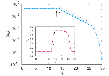
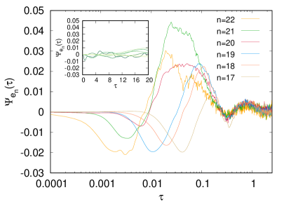
Figure 6 shows the energy spectrum, $\langle e_{n}\rangle$, and the energy flux, $\Pi_{n}$, (see inset): energy equipartition and zero energy flux obtained for shells smaller than the forced ones are good indicators of statistical equilibrium. At first we study the asymmetric correlation (11) to test the time asymmetry of the energy evolution at scales below/above the forcing one. As shown in Fig. 7, $\Psi_{e_{n}}(\tau)$ for $n>n_{f}$ (main panel) is akin to the results of Fig. 1(a) obtained with the usual large scale forcing, while for $n<n_{f}$ (see inset) is statistically compatible with zero, as expected in an equilibrium regime (Fig. 1(b)). Then we investigate the relaxation of an energy perturbation, either perturbing a shell $m>n_{f}$ (i.e. in the energy cascade range) or a shell $m<n_{f}$ (i.e. at scales larger than the forcing scale). Figure 8(a) displays the normalized RFs, i.e. the relative energy deviations, when the perturbed shell is larger than the forced ones, and their behavior retain the features shown by both forward and backward normalized RFs. Conversely, Fig. 8(b) refers to the case where the perturbation acts on a shell smaller than forced ones: as in the inviscid model, all RFs are positive and reach a common asymptote whose value is again found, in first approximation, by assuming energy equipartition among the degrees of freedom.

Summarizing, the behavior of both the asymmetric correlation and the energy response functions gives strong evidence that, in the shell model, the physics of the scales larger than the forcing one is compatible with the equilibrium as in the inviscid shell model. We remark, however, that there could be some properties which can deviate from equilibrium. The dynamics clearly does not preserve neither the energy nor the helicity and it is unclear what will be the effect on, e.g., the spectrum at the scales which match the forcing scales. As discussed in Appendix C, in the inviscid case oscillations in the spectra are expected at the boundary given by the largest shell, this will be clearly modified by the presence of the forcing. A confirmation of this difference is found in the good estimate of the asymptotic value computed with the perfect-equipartition assumption: boundary correction appears not necessary (Fig. 8(b)). In Ref. [33] it was pointed out that there are detectable deviations from Gaussianity at scales larger than the forcing scale for the Navier-Stokes equations. We studied a similar quantity, namely the third order velocity correlation function (not shown), and we found it to vanish as also confirmed by the analogous of the Kàrmàn-Howarth-Monin equation for the shell model. This difference is likely due to the fact that the quadratic interaction term is local in shell models.

V Conclusions

In this work we used asymmetric time correlation functions and response functions to finite perturbations to ascertain the breaking of time reversal symmetry and asymmetries between the degrees of freedom in a simplified model for the energy cascade in turbulence, i.e. the Sabra shell model [22]. We focused on the energy of a given shell and showed that by looking at a suitable time correlation of the energy one can clearly distinguish the case of a forced shell model displaying the direct energy cascade of energy to the case of an unforced and inviscid model. In the latter case the asymmetric correlation vanishes (meaning time reversible dynamics) while in the former it is definitely different from zero and the behavior understandable in terms of the Richardson energy cascade scenario. Similarly, clear differences between equilibrium (inviscid-unforced case) and non-equilibrium (forced viscous case) physics are clearly detectable using the energy response function, that is, perturbing the energy at given shell and looking at the time relaxation of the energy at a distant shell (either above or below the perturbed one). A net difference is observed in the forced case while looking at shells larger (scales smaller) or smaller (scales larger) than the perturbed one, as a consequence of the average energy current from large to small scales. Here the main novelty with respect to previous studies has been to perturb directly the energy and not the velocity. The quantities studied in this paper thus allow to observe (and, even if unnecessary, confirm) the celebrated Richardson cascade scenario from the perspective of non-equilibrium Statistical Mechanics. Finally, we considered the case of a shell model forced at intermediate scales so to allow for scrutinizing the behavior of both quantities at scales larger or smaller than the forcing scale. The emerging figure seems to confirm the view that scales larger than the forcing display properties which can be ascribed to the equilibrium physics of the unforced-inviscid model.

There are at least two interesting perspectives emerging from our study. Within the context of simplified models it would be interesting to explore, using the two tools we introduced, the shell model with the nonlinear term changed so to preserve energy and enstrophy, i.e. to mimic the two-dimensional Navier-Stokes equation [49, 50, 51]. In two dimensions an inverse (i.e. toward the large scales) energy cascade accompanied by a direct cascade of enstrophy takes place. However, in the shell model it has been shown that the latter is expected to display a spectrum akin to the enstrophy equipartition one [50]. Similarly to the extension of hydrodynamic turbulence to noninteger dimensions [52, 53], in shell models a tuning of the coupling parameter of nonlinear interactions can be associated to a continuous variation of the system dimensionality. An interplay of equilibrium and cascades is observed at varying this parameter [51, 54]. It is thus interesting to inquire whether the equilibrium or non-equilibrium character can be distinguished using the tools introduced in this work. Even more interesting would be to adapt our tools to the case of three-dimensional Navier-Stokes turbulence and, in particular, to explore their behavior at scales larger than the forcing scale where some features seem to be ascribable to equilibrium [30, 31, 32] while others show deviations from equilibrium [33, 34]. It could be not surprising, but surely very interesting, to discover that some properties are well captured by the equilibrium physics and others are not.

Appendix A Numerical details of simulations

The Sabra model (1-4) was integrated by means of a 4th order Runge-Kutta algorithm, with exact integration of the linear term (see e.g. [55]). In the turbulent case, the shell velocities were first initialized according to the scaling law: $|u_{n}|\sim k_{n}^{-1/2}$, and each complex velocity with a random phase. In the inviscid and unforced shell model we fixed the total energy $E=0.13$ and distributed it equally among all shells as $|u_{n}|=\sqrt{2E/N}$, with phase assigned randomly as well. Then, in both cases, we let the system evolve for a long enough transient of time (many turnover times) until a stationary state is reached, after which we start our measurements. As for the forcing $f_{n}$ in Eq. (1), we inject energy at scale $n_{f}$ and $n_{f}+1$ by imposing

$$f_{k}=\left\{\begin{array}[]{ll}\epsilon/(2u_{k}^{*})&\mathrm{for}\quad k=n_{f},n_{f}+1\\ 0&\mathrm{otherwise}\end{array}\right.$$ (20)

so that the energy power $\sum_{n}\Re(f_{n}u_{n}^{*})=\epsilon$ is constant. In all our simulation $\epsilon=1$.

Table 1 summarizes the parameters we used in the simulations.

Parameter	run-LSF	run-EQ	run-ISF
$\Delta t$	$5\cdot 10^{-5}$	$5\cdot 10^{-5}$	$10^{-5}$
$N$	24	15	30
$k_{0}$	$2^{-4}$	$2^{-4}$	$2^{-10}$
$n_{f}$	1	N.A.	13
$\nu$	$10^{-6}$	$0$	$5\cdot 10^{-7}$

Table 1: Values of the parameters used in numerical simulations. Run-LSF and Run-ISF correspond to the forced shell model, i.e. the turbulent case, with forcing at large scales or intermediate scales, respectively, while run-EQ denotes the equilibrium case, i.e. the unforced inviscid shell model. The parameters are the time step ($\Delta t$), the number of shells ($N$), the smallest wave number ($k_{0}$), the shell number where the forcing is acting ($n_{f}$), and the viscosity ($\nu$). In the forced runs the forcing acts on shell $n_{f}$ and $n_{f}+1$ in such a way to fix the energy injection rate to $\epsilon=1$.

Appendix B Issues on the numerical computation of asymmetric correlation functions $\Psi_{e_{n}}(t)$

In this Appendix we discuss some delicate issues about the numerical computation of the correlation functions (8) and its equivalent form (9). First of all, we can rewrite Eq. (9) as

$$\Phi_{x}(\tau)=\Theta_{x}(\tau)+\Psi_{x}(\tau)\,,$$ (21)

with $\Theta_{x}=\frac{1}{3}(\langle x^{3}(t+\tau)\rangle-\langle x^{3}(t)\rangle)$. Owing to the assumed stationarity of $x(t)$, it must hold $\Theta_{x}(\tau)=0$, and thus $\Phi_{x}(\tau)\equiv\Psi_{x}(\tau)$. However, in numerical evaluation, due to the way cancellations are realized, the two equivalent functions $\Psi_{x}$ and $\Phi_{x}$ have different pros and cons, as discussed below. In the following we will drop the subscript _x and the time dependence from the $x$ variable to ease the notation.

The obvious advantage of computing $\Psi(\tau)$ is that, especially at large $\tau$, it guarantees the cancellation of the term $\Theta(\tau)$, as this is automatically imposed. This can be appreciated from Fig. 9 where one can see that, at large $\tau$, the curves obtained computing $\Psi$ tend to be smoother than those obtained by computing $\Phi$, although both curves do convey the same result.

Figure 9: Correlation function $\Psi_{e_{n}}(\tau)$ and $\Phi_{e_{n}}(\tau)$ for $n=5,7,9$ versus $\tau$. Statistics is over $5\cdot 10^{5}$ samples. Inset: short time behavior ($\tau<1$) of the same correlation functions with inverted sign and in logarithmic $y$ scale. The dashed and dash-dotted lines denote respectively a linear and a cubic dependence on $\tau$. Statistics over $10^{6}$ samples. Notice that computing the running average (not shown) of $\langle e_{n}^{2}\dot{e_{n}}\rangle=d/dt\langle e_{n}^{3}\rangle/3$ one can clearly see the slow convergence to zero, which is responsible for the spurious linear behavior.

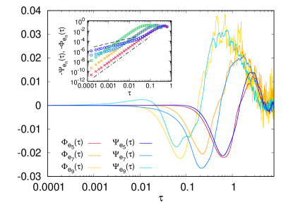
However, as it will be shown below, problems due to statistical convergence can manifest at small $\tau$, while the computation of $\Phi(\tau)$ is more efficient in ensuring the cancellations at small $\tau$’s. To realize such issue it is useful to expand in series $\Theta(\tau)$, $\Psi(\tau)$ and $\Phi(\tau)$:

$$\Theta(\tau) = \phantom{-}\langle x^{2}\dot{x}\rangle\tau+\frac{1}{2}\langle[2x\dot{x}^{2}+x^{2}\ddot{x}]\rangle\tau^{2}$$ (22)

$$+ \frac{1}{6}\langle[2\dot{x}^{3}+6x\dot{x}\ddot{x}+x^{2}\dddot{x}]\rangle\tau^{3}+\ldots$$

$$\Psi(\tau) = -\langle x^{2}\dot{x}\rangle\tau-\frac{1}{2}\langle[2x\dot{x}^{2}+x^{2}\ddot{x}]\rangle\tau^{2}$$ (23)

$$- \frac{1}{6}\langle[6x\dot{x}\ddot{x}+x^{2}\dddot{x}]\rangle\tau^{3}+\ldots\,.$$

$$\Phi(\tau) = \frac{1}{3}\langle\dot{x}^{3}\rangle\tau^{3}+\ldots\,.$$ (24)

Since $\Phi=\Psi$ also $\Psi(\tau)$ should behave the same way at small $\tau$. In order to see this it is useful to rewrite Eqs. (22-23) as

$$\Theta(\tau)\! = \!\frac{1}{3}\frac{d}{dt}\langle x^{3}\rangle\tau+\frac{1}{2}\frac{d}{dt}\langle[x^{2}\dot{x}]\rangle\tau^{2}+\frac{1}{6}\frac{d^{2}}{dt^{2}}\langle x^{2}\dot{x}\rangle\tau^{3}\phantom{\qquad}$$ (25)

$$\Psi(\tau) = -\frac{1}{3}\frac{d}{dt}\langle x^{3}\rangle\tau-\frac{1}{2}\frac{d}{dt}\langle[x^{2}\dot{x}]\rangle\tau^{2}$$ (26)

$$- \frac{1}{6}\left[\frac{d^{2}}{dt^{2}}\langle x^{2}\dot{x}\rangle-2\langle\dot{x}^{3}\rangle\right]\tau^{3}\,.$$

Now, clearly all the terms of the form $d^{k}/dt^{k}\langle[\ldots]\rangle$ should vanish by stationarity, so that $\Psi(\tau)=\frac{1}{3}\langle\dot{x}^{3}\rangle\tau^{3}$. However, the statistical convergence of $d^{k}/dt^{k}\langle[\ldots]\rangle\to 0$ may be hard to be obtained with a finite statistics leading to spurious $O(\tau)$ terms. The inset of Figure 9 does illustrate precisely this problem. As one can see the small $\tau$ behavior of $\Psi$ when computed for the energy of shell $5$ and $7$ starts with a spurious linear behavior and does recover the correct $\tau^{3}$ behavior only at sufficiently large $\tau$’s, while $\Phi$ does always display the correct $\tau^{3}$ dependence. For shell $9$ the two curves do coincide, this is simply due to the fact that shell $9$ is much faster than $7$ and $5$ so that statistical convergence, and thus the cancellations, can be realized more easily.

We conclude this appendix by noticing that in Ref.[8], it was reported a linear behavior at small $\tau$ for an experimental time series of a turbulent velocity flow. As discussed above, we strongly believe that the linear behavior have a spurious origin. It would thus be very interesting to re-analyze the data using $\Phi(\tau)$ instead of $\Psi(\tau)$ for confirmation.

Figure 10: Energy spectra of unperturbed and perturbed inviscid Sabra shell model. The fit on the equiparted region of the spectra, appertaining to the shells which are far enough from the lower boundary, lead to the value $R^{(\infty)}_{corr}$. Initial perturbation $\delta_{m=7}\simeq 1.79\cdot 10^{-3}$.

Appendix C Energy equipartition in the inviscid shell model

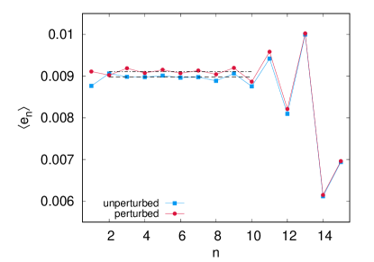
As discussed in App. A, for the inviscid shell model we start from an initially equiparted spectrum. However, as shown in Fig. 10, after a long average the energy spectrum shows clear departures from equipartition at large shell indexes, where oscillations do appear. A few more simulations (not shown), performed at changing the number of shells while keeping the energy per shell constant in the initial condition, demonstrate that the oscillations remain confined to the last 5-6 shells. Indeed by appropriately shifting the shell axis we observed that the oscillations do superimpose. This demonstrates that such oscillations are due to the boundary conditions which in the shell model, having a single variable per shell, are expected to have a stronger effect than in the truncated NSE. The main consequence of such oscillations is to alter the equipartition value of the energy far from the boundary, so to invalidate the naive expectation $R_{eq}^{(\infty)}=1/N$ for the asymptotic value of the energy response functions, as discussed in the main text. In order to determine the corrected (effective) value we have run a long simulation after a perturbation and computed the average spectrum: this way one can directly measure the energy shift in the far from boundary shells, which display equipartition (see Fig. 10). Due to this effect, the actual difference between the two equipartition values is larger than it would be in the case of perfect equipartition, meaning that the asymptotic value of $R_{m,n}(t)$ is slightly larger than expected (see Figure 4(b)).

Appendix D Initial time-derivatives of $R_{m,n}(t)$

In this Appendix we focus on the initial time derivatives of the energy response functions, showing that they provide information on the direction of the average energy flux among shells (where present).

From Eqs. (1-4) we can derive the following equation for the rate of change of energy at shell $n$:

$$\frac{de_{n}}{dt}=I_{n}+T_{n}+D_{n}\,,$$ (27)

where the three terms are the input power $I_{n}=\Re\{f_{n}u_{n}^{*}\}$, the non-linear transfer of energy

$$T_{n}=-[\Delta_{n+1}-\tfrac{1}{2}\Delta_{n}-\tfrac{1}{2}\Delta_{n-1}]\ ,$$ (28)

and the dissipated power $D_{n}=-\nu k_{n}^{2}|u_{n}|^{2}=-\nu k_{n}^{2}e_{n}$. For the sake of readability we omitted the time dependence in all the dynamical quantities. The transfer term explicitly shows that, by construction of the model, energy is directly exchanged between neighbors and next-to-neighbors shells, i.e. within a “range” (or distance) $2$. The real quantities $\Delta_{n}$, defined as $\Delta_{n}=k_{n}\Im\{u^{*}_{n-1}u^{*}_{n}u_{n+1}\}$ (see also Eq. (6)), play a key role in the following argument.

In both inviscid and turbulent cases (assuming in the latter to restrict ourselves in the inertial range so that the forcing is absent and the dissipation can be neglected) we can express the initial time derivative of $R_{m,n}$ using (27) as follows:

$$\frac{dR_{m,n}}{dt}\bigg{\rvert}_{t=0}=\frac{1}{\delta_{m}}\left[\overline{T^{\prime}_{n}(t)}-\overline{T_{n}(t)}\right]\bigg{\rvert}_{t=0}\ ,$$ (29)

where primed quantities refer to the perturbed system.

Let us start from the inviscid case. As shown in the inset of Fig. 4b, the time-derivative of $R_{m,n}$ is zero for $t=0$ for any $n$, which can be understood as follows. Clearly, if $|n-m|>2$ the perturbed shell $m$ does not directly interact with shell $n$, which is thus unaware of the perturbation for some time and, consequently, $\displaystyle dR_{m,n}/dt\big{\rvert}_{t=0}=0$. On the other hand if $|m-n|\leq 2$ the shell $n$ will in principle be affected by energy perturbation via the non-linear term. However, at equilibrium, we should expect the shell velocities to be statistically independent and Gaussian. Now, by using Eq. (27) with $I_{n}=D_{n}=0$, for $n=m+1$ it is easy to derive that

$$\frac{dR_{m,m+1}}{dt}\bigg{\rvert}_{t=0} \propto \tfrac{1}{2}(\overline{\delta\Delta_{m+1}}+\overline{\delta\Delta_{m}})\bigg{\rvert}_{t=0}\ .$$ (30)

where $\delta\Delta_{m}=k_{m}\Im\{u^{*}_{m-1}\delta u^{*}_{m}u_{m+1}\}$ and $\delta\Delta_{m+1}=k_{m+1}\Im\{\delta u^{*}_{m}u^{*}_{m+1}u_{m+2}\}$, and in general $\delta f$ denotes the difference between variable $f$ in the perturbed and unperturbed systems. Under the assumption that the average over many realization is equivalent to the statistical average, one finds that the triple moments factorize into the product of three single moments, two of which are zero. With the same reasoning one can conclude that the derivative should be zero also for $n=m-2,m-1$ and $m+2$.

$n$	R.h.s. of (32)
$m-2$	$-\overline{\alpha_{m}\Delta_{m-1}}\big{\rvert}_{t=0}<0$
$m-1$	$\overline{\alpha_{m}\left[\tfrac{1}{2}\Delta_{m-1}-\Delta_{m}\right]}\big{\rvert}_{t=0}<0$
$m+1$	$\overline{\alpha_{m}\left[\tfrac{1}{2}\Delta_{m}+\tfrac{1}{2}\Delta_{m+1}\right]}\big{\rvert}_{t=0}>0$
$m+2$	$\overline{\alpha_{m}\tfrac{1}{2}\Delta_{m+1}}\big{\rvert}_{t=0}>0$

Table 2: Initial time derivatives of $R_{m,n}(t)$ for $|n-m|\leq 2$.

We now discuss the turbulent case. For $|m-n|>2$ the same reasoning relying on the distance between perturbation and response applies, so that the initial derivatives of the RFs should be zero. For $|m-n|\leq 2$, one can construct the following argument. First, we rewrite the perturbed velocity (17) in terms of $u_{m}$ as $u^{\prime}_{m}=\sqrt{1+{\delta_{m}}/{e_{m}}}u_{m}$, so that

$$\delta u_{m}\!=\!(u^{\prime}_{m}\!-\!u_{m})\!=\!\left(\sqrt{1+\frac{\delta_{m}}{e_{m}}}\!-\!1\right)u_{m}\!\equiv\!\alpha_{m}u_{m}\,,$$ (31)

where we notice that $\alpha_{m}$ is a real positive quantity for $\delta_{m}>0$. Then, the equation (29) can be explicitly written as:

$$\delta_{m}\frac{dR_{m,n}}{dt}\bigg{\rvert}_{t=0}\!\!\!=\!-\!\biggl{[}\overline{\delta\Delta_{n+1}}\!-\!\tfrac{1}{2}\overline{\delta\Delta_{n}}\!-\!\tfrac{1}{2}\overline{\delta\Delta_{n-1}}\biggr{]}\bigg{\rvert}_{t=0}\,,$$ (32)

where

$$\delta\Delta_{n}\big{\rvert}_{t=0}\!=\!k_{n}\Im\biggl{[}\delta_{m,n-1}\alpha_{n-1}u^{*}_{n-1}u^{*}_{n}u_{n+1}\!$$ (33)

$$+\!\delta_{m,n}\ \alpha_{n}u^{*}_{n-1}u^{*}_{n}u_{n+1}+\delta_{m,n+1}\alpha_{n+1}u^{*}_{n-1}u^{*}_{n}u_{n+1}\biggr{]}$$

where the Kronecker delta $\delta_{a,b}$ imposes that at least one of the three shell velocities involved has to be the initially-perturbed one, otherwise there will be no contribution, as seen in the previous case.

Computing the sign of the initial time derivative of the RFs amounts to studying terms of the kind (indices omitted):

$$\overline{\delta\Delta}\sim k\overline{\alpha\Im\bigl{\{}uuu\bigr{\}}}=\overline{\alpha\Delta},$$ (34)

but $\alpha$ is positive by definition (see Eq. (31)), and it can be shown [22] that $\langle\Delta\rangle$ is positive on average, as it is related to the energy flux (6). Again we will assume that $\overline{\Delta}=\langle\Delta\rangle$.

Once established this result let us reconsider (32) and (33). In Table 2 we explicitly write the non-zero terms, when varying $n$ in the range of indices we are studying. Given that $\overline{\Delta_{n}}>0$, at least for $n$ in the inertial range, we have that backward RFs start with negative slope, while forward ones with positive slope. Concerning the case $n=m-1$, where the sign of the expression is not as straight-forward as the others, the negativity of the r.h.s. comes from an explicit result found in Eq. (16) of [22].

References

- Kubo et al. [2012] R. Kubo, M. Toda, and N. Hashitsume, Statistical physics II: nonequilibrium statistical mechanics, Vol. 31 (Springer Science & Business Media, 2012).
- Livi and Politi [2017] R. Livi and P. Politi, Nonequilibrium statistical physics: a modern perspective (Cambridge University Press, 2017).
- Ruelle [1996] D. Ruelle, Positivity of entropy production in nonequilibrium statistical mechanics, J. Stat. Phys. 85, 1 (1996).
- Seifert [2012] U. Seifert, Stochastic thermodynamics, fluctuation theorems and molecular machines, Rep. Prog. Phys. 75, 126001 (2012).
- Peliti and Pigolotti [2021] L. Peliti and S. Pigolotti, Stochastic Thermodynamics: An Introduction (Princeton University Press, 2021).
- Lebowitz and Spohn [1999] J. L. Lebowitz and H. Spohn, A Gallavotti–Cohen-type symmetry in the large deviation functional for stochastic dynamics, J. Stat. Phys. 95, 333 (1999).
- Pomeau [1982] Y. Pomeau, Symétrie des fluctuations dans le renversement du temps, J. Phys. France 43, 859 (1982).
- Josserand et al. [2017] C. Josserand, M. Le Berre, T. Lehner, and Y. Pomeau, Turbulence: Does energy cascade exist?, J. Stat. Phys. 167, 596 (2017).
- Xu et al. [2014] H. Xu, A. Pumir, G. Falkovich, E. Bodenschatz, M. Shats, H. Xia, N. Francois, and G. Boffetta, Flight–crash events in turbulence, Proc. Nat. Acad. Scie. 111, 7558 (2014).
- Zwanzig [2001] R. Zwanzig, Nonequilibrium statistical mechanics (Oxford University Press, 2001).
- Marconi et al. [2008] U. M. B. Marconi, A. Puglisi, L. Rondoni, and A. Vulpiani, Fluctuation–dissipation: Response theory in statistical physics, Phys. Rep. 461, 111 (2008).
- Sarra et al. [2021] C. Sarra, M. Baldovin, and A. Vulpiani, Response and flux of information in extended nonequilibrium dynamics, Phys. Rev. E 104, 024116 (2021).
- Rose and Sulem [1978] H. Rose and P. Sulem, Fully developed turbulence and statistical mechanics, J. Phys. France 39, 441 (1978).
- Frisch [1995] U. Frisch, Turbulence: the legacy of A. N. Kolmogorov (Cambridge University Press, 1995).
- Falkovich and Sreenivasan [2006] G. Falkovich and K. R. Sreenivasan, Lessons from hydrodynamic turbulence, Phys. Today 59, 43 (2006).
- Bohr et al. [1998] T. Bohr, M. H. Jensen, G. Paladin, and A. Vulpiani, Dynamical systems approach to turbulence (Cambridge University Press, 1998).
- Biferale [2003] L. Biferale, Shell models of energy cascade in turbulence, Annu. Rev. Fluid Mech. 35, 441 (2003).
- Ditlevsen [2010] P. D. Ditlevsen, Turbulence and shell models (Cambridge University Press, 2010).
- Ottinger and Carati [1996] J.-L. Ottinger and D. Carati, Relation between information transfer and structure function in shell models, Phys. Rev. E 53, 601 (1996).
- Biferale et al. [1999] L. Biferale, G. Boffetta, A. Celani, and F. Toschi, Multi-time, multi-scale correlation functions in turbulence and in turbulent models, Physica D 127, 187 (1999).
- Cencini et al. [2017] M. Cencini, L. Biferale, G. Boffetta, and M. De Pietro, Time irreversibility and multifractality of power along single particle trajectories in turbulence, Phys. Rev. Fluids 2, 104604 (2017).
- L’vov et al. [1998] V. S. L’vov, E. Podivilov, A. Pomyalov, I. Procaccia, and D. Vandembroucq, Improved shell model of turbulence, Phys. Rev. E 58, 1811 (1998).
- Biferale et al. [2001] L. Biferale, I. Daumont, G. Lacorata, and A. Vulpiani, Fluctuation-response relation in turbulent systems, Phys. Rev. E 65, 016302 (2001).
- Matsumoto et al. [2021] T. Matsumoto, M. Otsuki, T. Ooshida, and S. Goto, Correlation function and linear response function of homogeneous isotropic turbulence in the eulerian and lagrangian coordinates, J. Fluid Mech. 919, A9 (2021).
- Kubo [1966] R. Kubo, The fluctuation-dissipation theorem, Rep. Progr. Phys. 29, 255 (1966).
- Lucarini and Colangeli [2012] V. Lucarini and M. Colangeli, Beyond the linear fluctuation-dissipation theorem: the role of causality, J. Stat. Mech. 2012, P05013 (2012).
- Kraichnan [1973] R. H. Kraichnan, Helical turbulence and absolute equilibrium, J. Fluid Mech. 59, 745 (1973).
- Cichowlas et al. [2005] C. Cichowlas, P. Bonaïti, F. Debbasch, and M. Brachet, Effective dissipation and turbulence in spectrally truncated Euler flows, Phys. Rev. Lett. 95, 264502 (2005).
- Murugan et al. [2021] S. D. Murugan, D. Kumar, S. Bhattacharjee, and S. S. Ray, Many-body chaos in thermalized fluids, Phys. Rev. Lett. 127, 124501 (2021).
- Dallas et al. [2015] V. Dallas, S. Fauve, and A. Alexakis, Statistical equilibria of large scales in dissipative hydrodynamic turbulence, Phys. Rev. Lett. 115, 204501 (2015).
- Alexakis and Brachet [2019] A. Alexakis and M.-E. Brachet, On the thermal equilibrium state of large-scale flows, J. Fluid Mech. 872, 594 (2019).
- Gorce and Falcon [2022] J.-B. Gorce and E. Falcon, Statistical equilibrium of large scales in three-dimensional hydrodynamic turbulence, Phys. Rev. Lett. 129, 054501 (2022).
- Ding et al. [2023] M. Ding, J.-H. Xie, and J. Wang, Departure from the statistical equilibrium of large scales in three-dimensional hydrodynamic turbulence, arXiv preprint arXiv:2308.15292 (2023).
- Hosking and Schekochihin [2023] D. N. Hosking and A. A. Schekochihin, Emergence of long-range correlations and thermal spectra in forced turbulence, J. Fluid Mech. 973, A13 (2023).
- Alexakis et al. [2023] A. Alexakis, S. Chibbaro, and G. Michel, Fluctuation relations at large scales in three-dimensional hydrodynamic turbulence, arXiv preprint 2311.14440 (2023), accepted on EPL DOI:10.1209/0295-5075/ad0eec.
- Onsager [1931] L. Onsager, Reciprocal relations in irreversible processes. i., Phys. Rev. 37, 405 (1931).
- De Groot and Mazur [1984] S. R. De Groot and P. Mazur, Non-equilibrium thermodynamics (Dover Publications, 1984).
- Matsumoto et al. [2014] T. Matsumoto, M. Otsuki, O. Takeshi, S. Goto, and A. Nakahara, Response function of turbulence computed via fluctuation-response relation of a langevin system with vanishing noise, Phys. Rev. E 89, 061002 (2014).
- Boffetta et al. [2003] G. Boffetta, G. Lacorata, S. Musacchio, and A. Vulpiani, Relaxation of finite perturbations: Beyond the fluctuation-response relation, Chaos 13, 806 (2003).
- Falcioni et al. [1990] M. Falcioni, S. Isola, and A. Vulpiani, Correlation functions and relaxation properties in chaotic dynamics and statistical mechanics, Phys. Lett. A 144, 341 (1990).
- Ruelle [1998] D. Ruelle, General linear response formula in statistical mechanics, and the fluctuation-dissipation theorem far from equilibrium, Phys. Lett. A 245, 220 (1998).
- Harada and Sasa [2005] T. Harada and S.-i. Sasa, Equality connecting energy dissipation with a violation of the fluctuation-response relation, Phys. Rev. Lett. 95, 130602 (2005).
- Harada and Sasa [2006] T. Harada and S.-i. Sasa, Energy dissipation and violation of the fluctuation-response relation in nonequilibrium langevin systems, Phys. Rev. E 73, 026131 (2006).
- Baldovin et al. [2021] M. Baldovin, L. Caprini, and A. Vulpiani, Handy fluctuation-dissipation relation to approach generic noisy systems and chaotic dynamics, Phys. Rev. E 104, L032101 (2021).
- Lucarini et al. [2017] V. Lucarini, F. Ragone, and F. Lunkeit, Predicting climate change using response theory: Global averages and spatial patterns, J. Stat. Phys. 166, 1036 (2017).
- Ghil and Lucarini [2020] M. Ghil and V. Lucarini, The physics of climate variability and climate change, Rev. Mod. Phys. 92, 035002 (2020).
- Biferale et al. [2017] L. Biferale, A. A. Mailybaev, and G. Parisi, Optimal subgrid scheme for shell models of turbulence, Phys. Rev. E 95, 043108 (2017).
- Cameron et al. [2017] A. Cameron, A. Alexakis, and M.-É. Brachet, Effect of helicity on the correlation time of large scales in turbulent flows, Phys. Rev. Fluids 2, 114602 (2017).
- Aurell et al. [1994] E. Aurell, G. Boffetta, A. Crisanti, P. Frick, G. Paladin, and A. Vulpiani, Statistical mechanics of shell models for two-dimensional turbulence, Phys. Rev. E 50, 4705 (1994).
- Ditlevsen and Mogensen [1996] P. D. Ditlevsen and I. A. Mogensen, Cascades and statistical equilibrium in shell models of turbulence, Phys. Rev. E 53, 4785 (1996).
- Gilbert et al. [2002] T. Gilbert, V. S. L’vov, A. Pomyalov, and I. Procaccia, Inverse cascade regime in shell models of two-dimensional turbulence, Phys. Rev. Lett. 89, 074501 (2002).
- L’vov et al. [2002] V. S. L’vov, A. Pomyalov, and I. Procaccia, Quasi-gaussian statistics of hydrodynamic turbulence in dimensions, Phys. Rev. Lett. 89, 064501 (2002).
- Frisch et al. [2012] U. Frisch, A. Pomyalov, I. Procaccia, and S. S. Ray, Turbulence in noninteger dimensions by fractal fourier decimation, Phys. Rev. Lett. 108, 074501 (2012).
- Tom and Ray [2018] R. Tom and S. S. Ray, Revisiting the SABRA model: Statics and dynamics, EPL 120, 34002 (2018).
- Biferale et al. [2018] L. Biferale, M. Cencini, M. De Pietro, G. Gallavotti, and V. Lucarini, Equivalence of nonequilibrium ensembles in turbulence models, Phys. Rev. E 98, 012202 (2018).