Nonlinear redshift space distortion in halo ellipticity correlations:
Analytical model and $N$-body simulations

Abstract

We present an analytic model of nonlinear correlators of galaxy/halo ellipticities in redshift space. The three-dimensional ellipticity field is not affected by the redshift-space distortion (RSD) at linear order, but by the nonlinear one, known as the Finger-of-God effect, caused by the coordinate transformation from real to redshift space. Adopting a simple Gaussian damping function to describe the nonlinear RSD effect and the nonlinear alignment model for the relation between the observed ellipticity and underlying tidal fields, we derive analytic formulas for the multipole moments of the power spectra of the ellipticity field in redshift space expanded in not only the associated Legendre basis, a natural basis for the projected galaxy shape field, but also the standard Legendre basis, conventionally used in literature. The multipoles of the corresponding correlation functions of the galaxy shape field are shown to be expressed by a simple Hankel transform, as is the case for those of the conventional galaxy density correlations. We measure these multipoles of the power spectra and correlation functions of the halo ellipticity field using large-volume $N$-body simulations. We then show that the measured alignment signals can be better predicted by our nonlinear model than the existing linear alignment model. The formulas derived here have already been used to place cosmological constraints using from the redshift-space correlation functions of the galaxy shape field measured from the Sloan Digital Sky Survey Okumura and Taruya (2023).

I Introduction

Intrinsic alignments (IAs) of orientations of galaxies with the surrounding large-scale structure are considered a main source of systematics in cosmological gravitational lensing surveys Heavens et al. (2000); Croft and Metzler (2000); Lee and Pen (2000); Pen et al. (2000); Catelan et al. (2001); Crittenden et al. (2002); Jing (2002); Hirata and Seljak (2004); Heymans et al. (2004); Mandelbaum et al. (2006); Hirata et al. (2007); Okumura et al. (2009); Joachimi et al. (2011); Li et al. (2013); Singh et al. (2015); Tonegawa et al. (2018); Tonegawa and Okumura (2022) (see also Troxel and Ishak (2015); Joachimi et al. (2015); Kirk et al. (2015); Kiessling et al. (2015); Lamman et al. (2023) for reviews). The IA effect has also been attracting attention as a cosmological probe complimentary to the conventional galaxy clustering. It was pointed out that measurements of IAs in three dimensions can be used as dynamical and geometric probes of cosmology, with redshift-space distortions and baryon acoustic oscillations (BAO) (Chisari and Dvorkin, 2013; Okumura et al., 2019; Taruya and Okumura, 2020; Okumura and Taruya, 2022; Chuang et al., 2022). Further theoretical studies have shown that the measurements can be also used as probes of primordial non-Gaussianity (Schmidt et al., 2015; Chisari et al., 2016; Akitsu et al., 2021a), gravitational waves (Schmidt et al., 2014; Chisari et al., 2014; Biagetti and Orlando, 2020; Akitsu et al., 2023a), neutrino masses (Lee et al., 2023), statistical isotropy (Shiraishi et al., 2023) and gravitational redshifts (Zwetsloot and Chisari, 2022; Saga et al., 2023). Recently, observational constraints on cosmological models have been placed by measuring IAs of galaxies from the Sloan Digital Sky Survey (SDSS) (Okumura and Taruya, 2023; Kurita and Takada, 2023; Xu et al., 2023). More significant contributions on the cosmological constraints are expected by observations of the IA of galaxies in ongoing and upcoming galaxy redshift surveys with a better imaging quality Takada et al. (2014); DESI Collaboration et al. (2016); Euclid Collaboration et al. (2020).

In order to maximize the cosmological information encoded in the IA of galaxies, one needs to develop accurate non-linear models of IA statistics in full three dimensions. While modeling of the nonlinear power spectrum in redshift has been extensively performed for the galaxy density field (e.g., Peacock and Dodds, 1994; Park et al., 1994; Scoccimarro, 2004; Matsubara, 2008; Taruya et al., 2010; Seljak and McDonald, 2011; Okumura et al., 2015), there are fewer studies for the galaxy ellipticity field. The simplest model for the IA statistics is the linear alignment (LA) model, which linearly relates the ellipticity field to the tidal gravitational field Catelan et al. (2001); Hirata and Seljak (2004); Okumura et al. (2019); Okumura and Taruya (2020). The model beyond the LA model, nonlinear alignment (NLA) model as well as the nonlinear shape bias model have been studied Blazek et al. (2015); Schmitz et al. (2018); Blazek et al. (2019); Vlah et al. (2020); Taruya and Akitsu (2021); Matsubara (2022a, b, 2023); Bakx et al. (2023); Akitsu et al. (2023b); Maion et al. (2023). However, the modeling of the IA statistics in three dimensions requires an understanding of the nonlinear redshift-space distortion (RSD) effect on them Jackson (1972); Kaiser (1987), which is not as trivial as the nonlinearities above: Refs. Blazek et al. (2011); Chisari and Dvorkin (2013) had included the linear Kaiser factor into the redshift-space ellipticity field but later Ref. Singh et al. (2015) pointed out that the ellipticity field is not affected by the linear RSD. This argument is no longer valid once nonlinearities of IA are taken into account. It has been shown by Refs. Matsubara (2022b); Chen and Kokron (2023) in their analytical models that the ellipticity field is indeed affected by the nonlinear RSD effect. The accuracy of the models including the nonlinear RSD effect is still unclear because they have not been tested against the measurements from $N$-body simulations (but see Ref. Okumura and Taruya (2023) which provided the direct comparison with the observed result).

In this paper, we derive formulas of nonlinear intrinsic alignment statistics in redshift space where the nonlinear RSD effect is taken into account as a Gaussian damping function. We provide phenomenological formulas of both the IA power spectra and correlation functions. Conventionally, the IA correlations are expanded in terms of the (standard) Legendre polynomials Singh and Mandelbaum (2016); Okumura and Taruya (2020); Kurita et al. (2021). However, it was pointed out by Ref. Kurita and Takada (2022) that the IA statistics which contain the the geometric factor due to the projection of the intrinsic shape along the line of sight are more naturally expanded in terms of the associated Legendre polynomials rather than the standard Legendre ones (see also Ref. (Saga et al., 2023; Shi et al., 2023; Singh et al., 2023)). Thus, we provide our formulas expanded by both standard and associated Legendre polynomials. Note that the formulas derived here have already been used to place cosmological constraints from the Sloan Digital Sky Survey in Ref. Okumura and Taruya (2023).

Before proceeding to the next section, we note that we assume the linear and scale-independent bias for both the density and shape fields throughout the paper. The nonlinear shape bias has been investigated in real space (e.g., Schmitz et al. (2018); Akitsu et al. (2021b); Bakx et al. (2023); Akitsu et al. (2023b)). Incorporating the nonlinear bias effect into theoretical predictions of redshift-space IA statistics will be presented in the future work (but see Ref. Taruya and Akitsu (2021) for the impacts of nonlinear bias on the super-sample effects).

The rest of this paper is organized as follows. In Section II we describe general forms of the nonlinear power spectra of the ellipticity field in redshift space. Sections III and IV present the analytical model for the multipole moments of the IA power spectra and correlation functions, taking into account the nonlinear RSD and alignment effects. In Section V we presents the results of numerical calculations for the nonlinear RSD model of IA statistics. Our models for the IA statistics are tested against the measurements from $N$-body simulations in Section VI. Our conclusions are given in Section VII. The higher-order terms that do not contain linear contributions are provided in Appendix A. The expressions at the linear theory limit are provided in Appendix B.

Throughout the paper, we assume the spatially flat $\Lambda$CDM model as our fiducial model Planck Collaboration et al. (2016): $\Omega_{\rm m}=1-\Omega_{\rm DE}=0.315$, $\Omega_{K}=0$, $w_{0}=-1$, $w_{a}=0$, $H_{0}=67.3~{}[{\rm km/s/Mpc}]$ and the present-day value of $\sigma_{8}$ to be $\sigma_{8}=0.8309$.

II Galaxy density and ellipticity power spectra in redshift space

In this paper, we consider redshift-space correlators of the galaxy/halo ellipticity field with itself as well as with the density field. The positions of objects in three-dimensional galaxy surveys are sampled by their redshifts and are therefore displaced along the line of sight by their peculiar velocities, known as redshift-space distortions (RSD). The position of distant objects in real space, $\bm{x}$, is mapped to the one in redshift space, $\bm{s}$, as $\bm{s}=\bm{x}+\frac{v_{z}(\bm{x})}{aH(z)}\hat{\bm{z}}$, where $v_{z}(\bm{x})=\bm{v}(\bm{x})\cdot\hat{\bm{z}}$, $\bm{v}(\bm{x})$ is the peculiar velocity, $H(z)$ is the Hubble parameter at redshift $z$, $a=(1+z)^{-1}$ is the scale factor, and hat denotes a unit vector and $\hat{\bm{z}}$ is pointing the observer’s line of sight, namely, $\hat{\bm{z}}=\hat{\bm{s}}=\hat{\bm{x}}$.

II.1 Galaxy density field

Density perturbations of galaxies/halos are defined by the density contract from the mean $\bar{\rho}_{g}$,

$$\delta_{g}(\bm{x})\equiv\rho_{g}(\bm{x})/\bar{\rho}_{g}-1.$$ (1)

Through the real-to-redshift space mapping, the redshift-space density field of galaxies is given by (Scoccimarro, 2004; Taruya et al., 2010; Seljak and McDonald, 2011):

$$1+\delta_{g}^{S}(\bm{s})=\int d^{3}\bm{x}\int\frac{d^{3}\bm{k}}{(2\pi)^{3}}e^{-i\bm{k}\cdot[\bm{s}-\bm{x}+fu_{z}(\bm{x})\hat{\bm{z}}]}$$

$$\times[1+\delta_{g}(\bm{x})],$$ (2)

where $u_{z}(\bm{x})=-v_{z}(\bm{x})/(faH)$ and the superscript $S$ denotes a quantity defined in redshift space. The quantity $f$ is the growth rate parameter to characterize the evolution of the density perturbation, defined as

$$f(z)=-\frac{d\ln D(z)}{d\ln(1+z)}=\frac{d\ln D(a)}{d\ln a},$$ (3)

where $D(z)$ is the linear growth factor of the perturbation, $D(z)=\delta_{m}(\bm{x};z)/\delta_{m}(\bm{x};0)$. Via the Fourier transform,

$$\delta_{g}^{S}(\bm{k}) =\int d^{3}\bm{s}e^{-i\bm{k}\cdot\bm{s}}\delta_{g}^{S}(\bm{s})$$

$$=\int d^{3}\bm{x}e^{i\bm{k}\cdot[\bm{x}-fu_{z}(\bm{x})\hat{\bm{z}}]}\left[\delta_{g}(\bm{x})-f\nabla_{z}u_{z}(\bm{x})\right].$$ (4)

The galaxy auto-power spectrum, $P_{gg}^{S}(\bm{k})$, with the most general form under the plane-parallel approximation can be written as Scoccimarro et al. (1999); Scoccimarro (2004)

$$P_{gg}^{S}(\bm{k}) =\int d^{3}\bm{r}e^{i\bm{k}\cdot\bm{r}}\bigl{\langle}e^{-ifk\mu_{\bm{k}}\Delta u_{z}}\bigr{.}$$

$$\bigl{.}\times\left[\delta_{g}(\bm{x})+f\nabla_{z}u_{z}(\bm{x})\right]\left[\delta_{g}(\bm{x}^{\prime})+f\nabla_{z}u_{z}(\bm{x}^{\prime})\right]\bigr{\rangle},$$ (5)

where $\bm{r}=\bm{x}-\bm{x}^{\prime}$ and $\Delta u_{z}=u_{z}(\bm{x})-u_{z}(\bm{x}^{\prime})$.

II.2 Galaxy intrinsic ellipticity field

We use ellipticities of galaxies as a tracer of the 3-dimensional tidal field. Similarly to the density field, the redshift-space ellipticity field is described as (See Ref. Okumura et al. (2014) for a similar equation for the redshift-space velocity field)

$$\gamma_{ij}^{S}(\bm{s})=\int d^{3}\bm{x}\int\frac{d^{3}\bm{k}}{(2\pi)^{3}} e^{-i\bm{k}\cdot[\bm{s}-\bm{x}+fu_{z}(\bm{x})\hat{\bm{z}}]}\gamma_{ij}(\bm{x}),$$ (6)

which is translated into Fourier space as

$$\gamma_{ij}^{S}(\bm{k}) =\int d^{3}\bm{s}e^{-i\bm{k}\cdot\bm{s}}\gamma_{ij}^{S}(\bm{s})$$

$$=\int d^{3}\bm{x}e^{i\bm{k}\cdot[\bm{x}-fu_{z}(\bm{x})\hat{\bm{z}}]}\gamma_{ij}(\bm{x}).$$ (7)

The auto correlation of the ellipticity field and its cross correlation with the density field are, respectively,

$$P_{\gamma\gamma,ijkl}^{S}(\bm{k})= \int d^{3}\bm{r}e^{i\bm{k}\cdot\bm{r}}\bigl{\langle}e^{-ifk\mu_{\bm{k}}\Delta u_{z}}\gamma_{ij}(\bm{x})\gamma_{kl}(\bm{x}^{\prime})\bigr{\rangle},$$ (8)

$$P_{g\gamma,ij}^{S}(\bm{k})= \int d^{3}\bm{r}e^{i\bm{k}\cdot\bm{r}}\bigl{\langle}e^{-ifk\mu_{\bm{k}}\Delta u_{z}}\bigr{.}$$

$$\qquad\quad\bigl{.}\times\left[\delta_{g}(\bm{x})+f\nabla_{z}u_{z}(\bm{x})\right]\gamma_{ij}(\bm{x}^{\prime})\bigr{\rangle}.$$ (9)

Since the observed galaxy/halo shapes are projected onto the celestial sphere ($x-y$ plane), we consider the two traceless components as the observed shape field,

$$\left(\begin{array}[]{c}\gamma_{+}^{S}(\bm{k})\\ \gamma_{\times}^{S}(\bm{k})\end{array}\right)=\left(\begin{array}[]{c}\gamma_{xx}^{S}(\bm{k})-\gamma_{yy}^{S}(\bm{k})\\ 2\gamma_{xy}^{S}(\bm{k})\end{array}\right).$$ (14)

All the power spectra with this projected shape field can be expressed in terms of $P_{\gamma\gamma,ijkl}^{S}$ (Eq. 8) and $P_{g\gamma,ij}^{S}$ (Eq. 9), as

$$P_{g+}^{S}(\bm{k}) =P_{g\gamma,xx}^{S}(\bm{k})-P_{g\gamma,yy}^{S}(\bm{k}),$$ (15)

$$P_{g\times}^{S}(\bm{k}) =2P_{g\gamma,xy}^{S}(\bm{k}),$$ (16)

$$P_{++}^{S}(\bm{k}) =P_{\gamma\gamma,xxxx}^{S}(\bm{k})-2P_{\gamma\gamma,xxyy}^{S}(\bm{k})$$

$$\qquad\qquad+P_{\gamma\gamma,yyyy}^{S}(\bm{k}),$$ (17)

$$P_{\times\times}^{S}(\bm{k}) =4P_{\gamma\gamma,xyxy}^{S}(\bm{k}),$$ (18)

$$P_{+\times}^{S}(\bm{k}) =P_{\times+}^{S}(\bm{k})$$

$$=2\left[P_{\gamma\gamma,xxxy}^{S}(\bm{k})-P_{\gamma\gamma,yyxy}^{S}(\bm{k})\right],$$ (19)

$$P_{\pm}^{S}(\bm{k}) =P_{++}^{S}(\bm{k})\pm P_{\times\times}^{S}(\bm{k}),$$ (20)

We also define E-/B-modes, $\gamma_{(E,B)}$, which are the rotation-invariant decomposition of the ellipticity field Crittenden et al. (2002),

$$\gamma_{E}^{S}(\bm{k})+i\gamma_{B}^{S}(\bm{k})=e^{-2i\phi_{k}}\left[\gamma_{+}^{S}(\bm{k})+i\gamma_{\times}^{S}(\bm{k})\right],$$ (21)

where $\phi_{k}$ is the azimuthal angle of the wavevector projected on the celestial sphere. Then the power spectra of the E-/B-modes are expressed using those of $\gamma_{(+,\times)}^{S}(\bm{k})$ [Eqs. (15) – (19)]:

$$P_{gE}^{S}(\bm{k}) =\cos{(2\phi_{\bm{k}})}P_{g+}^{S}(\bm{k})+\sin{(2\phi_{\bm{k}})}P_{g\times}^{S}(\bm{k}),$$ (22)

$$P_{gB}^{S}(\bm{k}) =-\sin{(2\phi_{\bm{k}})}P_{g+}^{S}(\bm{k})+\cos{(2\phi_{\bm{k}})}P_{g\times}^{S}(\bm{k}),$$ (23)

$$P_{EE}^{S}(\bm{k}) =\cos^{2}{(2\phi_{\bm{k}})}P_{++}^{S}(\bm{k})+\sin^{2}{(2\phi_{\bm{k}})}P_{\times\times}^{S}(\bm{k})$$

$$\qquad+2\cos{(2\phi_{\bm{k}})}\sin{(2\phi_{\bm{k}})}P_{+\times}^{S}(\bm{k}),$$ (24)

$$P_{BB}^{S}(\bm{k}) =\sin^{2}{(2\phi_{\bm{k}})}P_{++}^{S}(\bm{k})+\cos^{2}{(2\phi_{\bm{k}})}P_{\times\times}^{S}(\bm{k})$$

$$\qquad-2\cos{(2\phi_{\bm{k}})}\sin{(2\phi_{\bm{k}})}P_{+\times}^{S}(\bm{k}).$$ (25)

Comparison of Eqs. (8) and (9) with Eq. (5) implies that the power spectra of the shape field in redshift space is affected by the Finger-of-God effect in the same way as those of the density field. We investigate the effect in the next section.

III Analytical model of nonlinear redshift-space distortion

III.1 Nonlinear alignment model

To relate the observed galaxy/halo shape field to the underlying tidal gravitational field, we use the linear alignment (LA) model, which assumes a linear relation between the intrinsic ellipticity and tidal field at the true three-dimensional position, namely without the line-of-sight displacement due to RSDs (Catelan et al., 2001; Hirata and Seljak, 2004). In Fourier space, the ellipticity field projected along the line of sight, $\hat{\bm{z}}$, is given by

$$\left(\begin{array}[]{c}\gamma_{+}(\bm{k})\\ \gamma_{\times}(\bm{k})\end{array}\right)=b_{K}\left(\begin{array}[]{c}k_{x}^{2}-k_{y}^{2}\\ 2k_{x}k_{y}\end{array}\right)\frac{\delta_{m}(\bm{k})}{k^{2}},$$ (30)

where $b_{K}$ represents the redshift-dependent coefficient of the intrinsic alignments which we refer to as the shape bias. We adopt the nonlinear alignment (NLA) model, which replaces the linear matter density field $\delta_{m}$ by the nonlinear one (Bridle and King, 2007). Furthermore, the redshift-space ellipticity field is multiplied by the damping function due to the nonlinear RSD effect as we will see below.

III.2 Phenomenological RSD model

To accurately describe the observed and simulated results of galaxy/halo ellipticity correlations in redshift space, the nonlinear RSD effect, known as the Finger-of-God (FoG), needs to be taken into account in the theoretical predictions. In Sec. II, we see that the expressions of power spectra involve the exponential factor in the ensemble average [see Eqs. (5), (8) and (9)], which is responsible for suppressing the power spectrum amplitude due to the randomness of the pair-wise velocity contributions. Although the impact of this exponential factor, coupled with the density and ellipticity fields, needs to be carefully treated in the statistical calculations, a dominant effect of this is phenomenologically but quantitatively described by imposing the factorized ansatz, i.e., $\langle e^{-ifk\mu_{k}\Delta u_{z}}\{\cdots\}\rangle\to\langle e^{-ifk\mu_{k}\Delta u_{z}}\rangle\langle\cdots\rangle$. Then, writing all the redshift-space power spectra in the previous subsection as $P_{X}^{S}(\bm{k})$, this ansatz leads to the following separable expression of the power spectra: Scoccimarro (2004) (see also Peacock and Dodds (1994); Park et al. (1994); Taruya et al. (2009); Okumura et al. (2012a)),

$$P_{X}^{S}(\bm{k})=\hat{P}_{X}^{S}(\bm{k})D_{\rm FoG}^{2}(fk\mu_{\bm{k}}\sigma_{\rm v}),$$ (31)

where $k=|\bm{k}|$, $\mu_{\bm{k}}=\hat{\bm{k}}\cdot\hat{\bm{z}}=k_{z}/k$ is the directional cosine between the observer’s line of sight and the wavevector $\bm{k}$. In this expression, the exponential factor $\langle e^{-ifk\mu_{\bm{k}}\Delta u_{z}}\rangle$ is identified with the function $D_{\rm FoG}^{2}$, and we model it as the zero-lag correlation characterized by the velocity dispersion, $\sigma_{\rm v}$.

Eq. (31) includes the redshift-space galaxy power spectrum proposed by Ref. Scoccimarro (2004) ($X=gg$). In this case, the function $\hat{P}_{gg}^{S}$ is given by

$$\hat{P}_{gg}^{S}(\bm{k})=b^{2}P_{\delta\delta}(k)+2bf\mu_{\bm{k}}^{2}P_{\delta\theta}(k)+f^{2}\mu_{\bm{k}}^{4}P_{\theta\theta}(k),$$ (32)

where $b$ is the linear galaxy bias (Kaiser, 1984), $P_{\delta\delta}$ and $P_{\theta\theta}$ are the nonlinear auto-power spectra of density and velocity divergence, respectively, and $P_{\delta\theta}$ is the their cross-power spectrum. In the linear theory limit, $P_{\delta\delta}=P_{\delta\theta}=P_{\theta\theta}$ and $D_{\rm FoG}=1$, and hence Equation (32) converges to the original Kaiser formula Kaiser (1987). The parameter $f$ quantifies the cosmological velocity field and the speed of structure growth, and thus is useful for testing a possible deviation of the gravity law from general relativity (Guzzo et al., 2008; Okumura et al., 2016). Under modified gravity models, even though the background evolution were the same as the $\Lambda$CDM model, the density perturbations would evolve differently (See, e.g., Ref. Matsumoto et al. (2020) for degeneracies between the expansion and growth rates for various gravity models). The relation of this phenomenological form with the general one in Eq. (5) was made in Ref. Taruya et al. (2010).

Adopting the NLA model, the cross-power spectra of the galaxy density and E-/B-mode fields and the auto-power spectra of the E-/B-mode fields are given by

$$\hat{P}_{gE}^{S}(\bm{k})=b_{K}(1-\mu_{\bm{k}}^{2})\left[bP_{\delta\delta}(k)+f\mu_{\bm{k}}^{2}P_{\delta\theta}(k)\right],$$ (33)

$$\hat{P}_{EE}^{S}(\bm{k})=b_{K}^{2}(1-\mu_{\bm{k}}^{2})^{2}P_{\delta\delta}(k),$$ (34)

$$\hat{P}_{gB}^{S}(\bm{k})=\hat{P}_{BB}^{S}(\bm{k})=0.$$ (35)

The power spectra of the E-mode, namely $P_{gE}^{S}$ and $P_{EE}^{S}$, are the main statistics to be tested in this paper. Our model for these statistics contain free parameters of ${\bm{\theta}}=(f,b,b_{K},\sigma_{\rm v})$.

When we analyze power spectra that are anisotropic along the line of sight and thus have $\mu_{\bm{k}}$ dependences, we commonly use the multipole expansion in terms of the Legendre polynomials, ${\cal L}_{\ell}(\mu_{\bm{k}})$, as Hamilton (1992); Okumura and Taruya (2020):

$$P_{X}^{S}(\bm{k})=\sum_{\ell:{\rm even}}P_{X,\ell}^{S}(k){\cal L}_{\ell}(\mu_{\bm{k}}),$$ (36)

where the coefficients $P_{X,\ell}^{S}(k)$ are given by

$$P_{X,\ell}^{S}(k)=\frac{2\ell+1}{2}\int^{1}_{-1}d\mu_{\bm{k}}P_{X}^{S}(k,\mu_{\bm{k}})\mathcal{L}_{\ell}(\mu_{\bm{k}}).$$ (37)

In this paper, we adopt a simple Gaussian function for the nonlinear RSD term, $D_{\rm FoG}(fk\mu_{\bm{k}}\sigma_{\rm v})=\exp{\left[-(fk\mu_{\bm{k}}\sigma_{\rm v})^{2}/2\right]}\equiv\exp{\left(-\alpha\mu_{\bm{k}}^{2}/2\right)}$, where $\alpha=(fk\sigma_{\rm v})^{2}$ . With this Gaussian function, all the multipole moments of the power spectra, i.e., $P_{X,\ell}^{S}(k)$, are expressed in a factorized form with the angular dependence encoded by

$$p^{(n)}(\alpha)\equiv\int^{1}_{-1}d\mu_{\bm{k}}\mu_{\bm{k}}^{2n}e^{-\alpha\mu_{\bm{k}}^{2}}.$$ (38)

The integral can be performed analytically as $p^{(n)}(\alpha)=\frac{\gamma(1/2+n,\alpha)}{\alpha^{1/2+n}},$ where $\gamma(n,\alpha)=\int^{\alpha}_{0}dt\ t^{n-1}e^{-t}$ is the incomplete gamma function of the first kind. All the formulas derived below are, thus, expressed in terms of the function $p^{(n)}(\alpha)$. The linear-theory limits of the formulas are derived by setting $\alpha=0$, $p^{(n)}(0)=\frac{2}{2n+1}$.

The expression of the multipole expansions for the nonlinear galaxy power spectra with the Gaussian damping function were derived by Refs. Taruya et al. (2009); Percival and White (2009). They are expressed in terms of $p^{(n)}(\alpha)$ as

$$P_{gg,\ell}^{S}(k) =b^{2}\mathcal{Q}_{gg,\ell}^{(0)}(\alpha)P_{\delta\delta}(k)+2bf\mathcal{Q}_{gg,\ell}^{(1)}(\alpha)P_{\delta\theta}(k)$$

$$\qquad\qquad\qquad+f^{2}\mathcal{Q}_{gg,\ell}^{(2)}(\alpha)P_{\theta\theta}(k).$$ (39)

The multipoles with $\ell=0,2,4$ contain non-zero contributions at linear scales. The functions $\mathcal{Q}_{gg,\ell}^{(n)}(\alpha)$ up to $\ell=4$ are given by

$$\mathcal{Q}_{gg,0}^{(n)}(\alpha) =\frac{1}{2}p^{(n)}(\alpha),$$ (40)

$$\mathcal{Q}_{gg,2}^{(n)}(\alpha) =\frac{5}{4}\left[3p^{(n+1)}(\alpha)-p^{(n)}(\alpha)\right],$$ (41)

$$\mathcal{Q}_{gg,4}^{(n)}(\alpha) =\frac{9}{16}\left[35p^{(n+2)}(\alpha)-30p^{(n+1)}(\alpha)\right.$$

$$\qquad\qquad\qquad\qquad\quad\left.+3p^{(n)}(\alpha)\right].$$ (42)

By taking the $\alpha\to 0$ limit, $\mathcal{Q}_{gg,\ell}(0)=0$ for $\ell>4$ and the linear RSD formulas are obtained Kaiser (1987).

III.3 E-mode cross- and auto-power spectra

Due to the geometric factor, $(1-\mu_{\bm{k}}^{2})$, arising from the projection of the shape field along the line of sight in Eqs. (33) and (34), the cross-power spectra of the galaxy density and E-mode shape fields (gE power) and auto-power spectra of the E-mode shape field (EE power) are more naturally expressed in the associated Legendre basis rather than in the standard Legendre basis,

$$P_{X}^{S}(\bm{k})=\sum_{\ell:{\rm even}}\widetilde{P}_{X,L}^{S}(k)\Theta_{L}^{m}(\mu_{\bm{k}}),$$ (43)

where $X=\{gE,EE\}$, $\Theta_{L}^{m}(\mu)$ is the normalized associated Legendre function related to the unnormalized one by $\Theta_{L}^{m}(\mu)=\sqrt{\frac{2\ell+1}{2}\frac{(L-m)!}{(L+m)!}}\mathcal{L}_{L}^{m}(\mu_{\bm{k}})$, so that it satisfies a simple orthonormal relation, $\int^{1}_{-1}d\mu\Theta_{L}^{m}(\mu)\Theta_{L^{\prime}}^{m}(\mu)=\delta_{LL^{\prime}},$ with $\delta_{LL^{\prime}}$ being the Kronecker’s delta. We added tilde to $P_{X,L}^{S}(k)$ to emphasize that they are the expansion coefficients of the normalized polynomials $\Theta_{L}^{m}(\mu_{\bm{k}})$. While the choice of $m$ in Eq. (43) is arbitrary, the expressions of the gE and EE power spectra become the simplest if one chooses $m=2$ and $4$, respectively Kurita and Takada (2022). Thus, in the following, $\widetilde{P}_{gE,L}^{S}(k)$ and $\widetilde{P}_{EE,L}^{S}(k)$ stand for the coefficients expanded by $\Theta_{L}^{m=2}$ and $\Theta_{L}^{m=4}$, respectively. We also provide the expression of the multipoles of the gE and EE power spectra expanded in terms of the standard Legendre polynomials, which used to be commonly considered theoretically but were found to be not direct observables in real surveys Kurita and Takada (2022).

All the multipoles of the power spectra considered in this subsection are summarized in Table 1. We present only the multipoles $\widetilde{P}_{X,L}^{S}$ and $P_{X,\ell}^{S}$ that contain linear-order contributions here, and the higher-order terms are provided in Appendix A up to $L=12$ and $\ell=12$, respectively. We can obtain the linear theory expressions by taking the $\alpha\to 0$ limit, and they are shown in Appendix B.

Table 1: Summary of the coordinate-independent alignment power spectra derived in section III. The functions $\widetilde{P}_{X,L}^{S}$ and $P_{X,\ell}^{S}$ are coefficients expanded in terms of the normalized associated Legendre polynomial $\Theta_{L}$ and standard Legendre polynomial $\mathcal{L}_{\ell}$, respectively.

Statistics		Definition		Fourier-space			Result (Fig.)
		(Eq.)		multipole	(Eq.)		Theory	Sim.
gE		$P_{gE}^{S}(\bm{k})$ (33)		$\widetilde{P}_{gE,L}^{S}$	(44)		1	6
				$P_{gE,\ell}^{S}$	(47)		2	7
EE		$P_{EE}^{S}(\bm{k})$ (34)		$\widetilde{P}_{EE,L}^{S}$	(51)		1	6
				$P_{EE,\ell}^{S}$	(53)		2	7

Using the function $p^{(n)}(\alpha)$ [Eq. (38)], the gE power spectrum, $\widetilde{P}_{gE,L}^{S}(k)$, is explicitly described as

$$\widetilde{P}_{gE,L}^{S}(k) =\int^{1}_{-1}d\mu_{\bm{k}}P_{gE}^{S}(k,\mu_{\bm{k}})\Theta_{L}^{m=2}(\mu_{\bm{k}})$$

$$=bb_{K}\mathcal{\widetilde{Q}}_{gE,L}^{(0)}(\alpha)P_{\delta\delta}(k)$$

$$\qquad\qquad+fb_{K}\mathcal{\widetilde{Q}}_{gE,L}^{(1)}(\alpha)P_{\delta\theta}(k),$$ (44)

where $L\geq m=2$. The two lowest multipoles, $\widetilde{P}_{gE,L}^{S}(k)$ with $L=2$ and $4$, contain linear-order contributions, and $\mathcal{Q}_{gE,L}^{(n)}(\alpha)$ are given by

$$\mathcal{\widetilde{Q}}_{gE,2}^{(n)}(\alpha) =\frac{\sqrt{15}}{4}\left[p^{(n)}(\alpha)-2p^{(n+1)}(\alpha)\right.$$

$$\qquad\qquad\left.+p^{(n+2)}(\alpha)\right],$$ (45)

$$\mathcal{\widetilde{Q}}_{gE,4}^{(n)}(\alpha) =\frac{3\sqrt{5}}{8}\left[-p^{(n)}(\alpha)+9p^{(n+1)}(\alpha)\right.$$

$$\qquad\qquad\left.-15p^{(n+2)}(\alpha)+7p^{(n+3)}(\alpha)\right].$$ (46)

Table 2: Same as Table 1 but for the coordinate-dependent alignment power spectra derived in section IV. The functions $P_{\ell m}^{X}$ are coefficients expanded in terms of the spherical harmonics $Y_{\ell m}$. The power spectra are used to derive the expressions for the corresponding correlation functions, $\xi_{X,\ell}^{S}$ and $\widetilde{\xi}_{X,L}^{S}$.

Statistics		Definition		Fourier-space			Configuration-space			Result (Fig.)
		(Eq.)		multipole	(Eq.)		multipole	(Eq.)		Theory	Sim.
II($+$)		$P_{+}^{S}(\bm{k})$ (59)		$P_{+,\ell}^{S}$	(65)		$\xi_{+,\ell}^{S}$	(66)			9
g$+$		$P_{g+}^{S}(\bm{k})$ (58)		$P_{\ell m}^{g+}$	(82)		$\widetilde{\xi}_{g+,L}^{S}$	(111)		1	8
							$\xi_{g+,\ell}^{S}$	(113)–(115)		2	9
II($-$)		$P_{-}^{S}(\bm{k})$ (59)		$P^{-}_{\ell m}$	(90)		$\widetilde{\xi}_{-,L}^{S}$	(112)		1	8
							$\xi_{-,\ell}^{S}$	(116)–(118)		2	9

When the gE power spectrum is expanded by the standard Legendre basis [Eq. (36)] instead of the associated Legendre basis, they are shown to be:

$$P_{gE,\ell}^{S}(k) =bb_{K}\mathcal{Q}_{gE,\ell}^{(0)}(\alpha)P_{\delta\delta}(k)$$

$$\qquad\qquad+fb_{K}\mathcal{Q}_{gE,\ell}^{(1)}(\alpha)P_{\delta\theta}(k),$$ (47)

where $\mathcal{Q}_{gE,\ell}^{(n)}$ which contain the linear contributions are given by

$$\mathcal{Q}_{gE,0}^{(n)}(\alpha) =\frac{1}{2}\left[p^{(n)}(\alpha)-p^{(n+1)}(\alpha)\right],$$ (48)

$$\mathcal{Q}_{gE,2}^{(n)}(\alpha) =-\frac{5}{4}\left[p^{(n)}(\alpha)-4p^{(n+1)}(\alpha)\right.$$

$$\qquad\left.+3p^{(n+2)}(\alpha)\right],$$ (49)

$$\mathcal{Q}_{gE,4}^{(n)}(\alpha) =\frac{9}{16}\left[3p^{(n)}(\alpha)-33p^{(n+1)}(\alpha)\right.$$

$$\qquad\left.+65p^{(n+2)}(\alpha)-35p^{(n+3)}(\alpha)\right].$$ (50)

Similarly to the gE power spectrum in Eq. (44), the EE auto-power spectrum expanded in terms of the associated Legendre polynomials, $\widetilde{P}_{EE,L}^{S}(k)$, is concisely described as

$$\widetilde{P}_{EE,L}^{S}(k) =\int^{1}_{-1}d\mu_{\bm{k}}P_{EE}^{S}(k,\mu_{\bm{k}})\Theta_{L}^{m=4}(\mu_{\bm{k}})$$

$$=b_{K}^{2}\mathcal{\widetilde{Q}}_{EE,L}(\alpha)P_{\delta\delta}(k),$$ (51)

where $L\geq m=4$. Only the lowest-order coefficient with $L=4$, $\mathcal{\widetilde{Q}}_{EE,4}$, contains the contribution in linear theory. The term is given by

$$\mathcal{\widetilde{Q}}_{EE,4}(\alpha) =\frac{3\sqrt{35}}{16}\left[p^{(0)}(\alpha)-4p^{(1)}(\alpha)+6p^{(2)}(\alpha)\right.$$

$$\qquad\qquad\left.-4p^{(3)}(\alpha)+p^{(4)}(\alpha)\right].$$ (52)

The multipole expansions of the EE power in terms of the standard Legendre polynomials are expressed as

$$P_{EE,\ell}^{S}(k) =b_{K}^{2}\mathcal{Q}_{EE,\ell}(\alpha)P_{\delta\delta}(k),$$ (53)

where

$$\mathcal{Q}_{EE,0}(k) =\frac{1}{2}\left[p^{(0)}(\alpha)-2p^{(1)}(\alpha)+p^{(2)}(\alpha)\right],$$ (54)

$$\mathcal{Q}_{EE,2}(k) =-\frac{5}{4}\left[p^{(0)}(\alpha)-5p^{(1)}(\alpha)+7p^{(2)}(\alpha)\right.$$

$$\qquad\quad\quad\quad\left.-3p^{(3)}(\alpha)\right],$$ (55)

$$\mathcal{Q}_{EE,4}(\alpha) =\frac{9}{16}\left[3p^{(0)}(\alpha)-36p^{(1)}(\alpha)+98p^{(2)}(\alpha)\right.$$

$$\qquad\quad\quad\quad\left.-100p^{(3)}(\alpha)+35p^{(4)}(\alpha)\right].$$ (56)

Numerical results of these nonlinear formulas are given in Sec. V and compared to the measurements from $N$-body simulations in Sec. VI.

IV Ellipticity correlation functions

In this section, we present multipole moments of the correlation functions of the projected galaxy/halo ellipticity field in redshift space. A two-point correlation function is related to the power spectrum by a Fourier transform,

$$\xi_{X}^{S}(\bm{r}) =\int\frac{d^{3}\bm{k}}{(2\pi)^{3}}P_{X}^{S}(\bm{k})\,e^{i\,\bm{k}\cdot\bm{r}}$$

$$=\int\frac{d^{3}\bm{k}}{(2\pi)^{3}}\hat{P}_{X}^{S}(\bm{k})D_{\rm FoG}^{2}(fk\mu_{\bm{k}}\sigma_{\rm v})\,e^{i\,\bm{k}\cdot\bm{r}}.$$ (57)

We start by considering the power spectra of the shape field, namely Eqs. (15)–(20). Following the model developed in Sec. III.2, the part $\hat{P}_{X}^{S}(\bm{k})$ in Eq. (31) are given by

$$\hat{P}_{g+}^{S}(\bm{k})=b_{K}k^{-2}(k_{x}^{2}-k_{y}^{2})\left[bP_{\delta\delta}(k)+f\mu_{\bm{k}}^{2}P_{\delta\theta}(k)\right],$$ (58)

$$\hat{P}_{\pm}^{S}(\bm{k})=b_{K}^{2}k^{-4}\left[(k_{x}^{2}-k_{y}^{2})^{2}\pm(2k_{x}k_{y})^{2}\right]P_{\delta\delta}(k),$$ (59)

$$\hat{P}_{g\times}^{S}(\bm{k})=\hat{P}_{+\times}^{S}(\bm{k})=\hat{P}_{\times+}^{S}(\bm{k})=0.$$ (60)

In the following, we derive the multipoles of the non-zero IA power spectra, $P_{g+}^{S}(\bm{k})$ and $P_{\pm}^{S}(\bm{k})$, and substitute them into Eq. (57). Following Ref. Kurita and Takada (2022), we express the inverse Hankel transform, as

$$\mathcal{H}_{\ell}^{-1}\left[g(k)\right](r)\equiv i^{\ell}\int\frac{k^{2}dk}{2\pi^{2}}j_{\ell}(kr)g(k).$$ (61)

Using this notation, the commonly-used multipole expansion of an anisotropic power spectrum is described as

$$\xi_{X}^{S}(\bm{r})=\sum_{\ell:{\rm even}}\xi_{X,\ell}^{S}(r){\cal L}_{\ell}(\mu_{s}),$$ (62)

where $\xi_{X,\ell}^{S}(r)=\mathcal{H}_{\ell}^{-1}\left[P_{X,\ell}^{S}(k)\right]$. The multipole components of the conventional galaxy density correlation function with the FoG Gaussian damping term (Eq. 39) are given by

$$\xi_{gg,\ell}^{S}(r) =b^{2}\Pi_{\delta\delta,\ell}^{gg(0)}(r)+2bf\Pi_{\delta\Theta,\ell}^{gg(1)}(r)$$

$$\qquad\qquad\qquad+f^{2}\Pi_{\Theta\Theta,\ell}^{gg(2)}(r),$$ (63)

where $\Pi_{X,\ell}^{Y(n)}(r)=\mathcal{H}_{\ell}^{-1}\left[\mathcal{Q}_{Y,\ell}^{(n)}(k)P_{X}(k)\right]$. In the linear theory limit ($\sigma_{\rm v}\to 0$), the equation is reduced to the Kaiser formula (Kaiser, 1987; Hamilton, 1992; Okumura and Jing, 2011).

In section IV.1, the model for the II($+$) correlation multipoles in terms of the standard Legendre polynomials is given. In section IV.2 we first provide the models for the GI and II($-$) multipoles in terms of the associated Legendre polynomials, and then those of the standard Legendre polynomials. Table 2 summarizes all the power spectra and correlation functions of the shape field considered in this section.

IV.1 II($+$) correlation functions

Since the II($+$) power spectrum, $P_{+}^{S}(\bm{k})$, is equivalent to the EE power spectrum, $P_{+}^{S}(\bm{k})=P_{EE}(\bm{k})$ [Eqs. (53) – (56)], the expression for the II($+$) spectrum expanded in terms of the standard Legendre polynomials, $P_{+,\ell}^{S}(k)$, can be written as

$$P_{+,\ell}^{S}(k) =b_{K}^{2}\mathcal{Q}_{+,\ell}(\alpha)P_{\delta\delta}(k),$$ (65)

where $\mathcal{Q}_{+,\ell}(\alpha)=\mathcal{Q}_{EE,\ell}(\alpha)$, and $\ell=0,2$ and $4$ multipoles contain the linear contributions. The II($+$) multipoles are given in a similar manner to the GG multipoles,

$$\xi_{+,\ell}^{S}(r) =b_{K}^{2}\Pi_{\delta\delta,\ell}^{+}(r),$$ (66)

where $\Pi_{\delta\delta,\ell}^{+}(r)=\mathcal{H}_{\ell}^{-1}\left[\mathcal{Q}_{+,\ell}(k)P_{\delta\delta}(k)\right]$. Again, taking $\sigma_{\rm v}\to 0$ limit leads to the linear theory formula of Ref. Okumura and Taruya (2020).

IV.2 GI and II($-$) correlation functions

To obtain the multipoles of the GI and II($-$) power spectra, we consider the spherical harmonic expansion of a power spectrum, $P_{X}^{S}(\bm{k})$, where $X=\{g+,-\}$,

$$P_{X}^{S}(\bm{k})=\sum_{\ell,m}P_{\ell m}^{X}(k)Y_{\ell m}^{*}(\hat{\bm{k}}),$$ (67)

where $P_{\ell m}^{X}(k)$ is the coefficients of the spherical harmonic expansion, given by

$$P_{\ell m}^{X}(k)=\int d^{2}\hat{\Omega}_{\bm{k}}P_{X}^{S}(\bm{k})Y_{\ell m}(\hat{\bm{k}}).$$ (68)

To compute $P_{\ell m}^{X}(k)$ explicitly, we first write the geometric factors in $P_{g+}^{S}(\bm{k})$ and $P_{-}^{S}(\bm{k})$ due to the projection in terms of the spherical harmonics, respectively, as

$$k^{-2}(k_{x}^{2}-k_{y}^{2})=\sqrt{\frac{8\pi}{15}}\Bigl{[}Y_{2,2}(\hat{k})+Y_{2,-2}(\hat{k})\Bigr{]}~{},$$ (69)

$$k^{-4}\left[(k_{x}^{2}-k_{y}^{2})^{2}-(2k_{x}k_{y})^{2}\right]$$

$$\qquad\qquad\qquad=\sqrt{\frac{128\pi}{315}}\Bigl{[}Y_{4,4}(\hat{k})+Y_{4,-4}(\hat{k})\Bigr{]}~{}.$$ (70)

Next, we also express the RSD factor, the integrand of Eq. (38), in terms of the spherical harmonics,

$$\mu_{\bm{k}}^{2n}e^{-\alpha\mu_{\bm{k}}^{2}} =\sum_{q=0}^{\infty}\,F_{2q}^{(n)}(\alpha)\,Y_{2q,0}(\hat{k}).$$ (71)

Using the orthogonality of the spherical harmonics, the coefficient $F_{q}^{(n)}(\alpha)$ is written as

$$F_{q}^{(n)}(\alpha) =2\pi\int^{1}_{-1}d\mu_{\bm{k}}\,\mu_{\bm{k}}^{2n}\,e^{-\alpha\mu_{\bm{k}}^{2}}Y_{q,0}(\hat{k}).$$ (72)

It is related to $p^{(n)}(\alpha)$ (Eq. 38) as $F^{(n)}_{0}=\sqrt{\pi}p^{(n)}$.

Substituting these equations into Eq. (31) with Eqs. (58) and (59) and then using Eq. (68), the functions $P_{\ell m}^{g+}(k)$ and $P^{-}_{\ell m}(k)$ are given by

$$P_{\ell m}^{g+}(k) =b_{K}\sqrt{\frac{8\pi}{15}}\sum_{q=0}\Bigl{[}bF_{2q}^{(0)}P_{\delta\delta}(k)+fF_{2q}^{(1)}P_{\delta\theta}(k)\Bigr{]}$$

$$\quad\times\int d^{2}\hat{\Omega}_{k}\Bigl{[}Y_{2,2}(\hat{k})+Y_{2,-2}(\hat{k})\Bigr{]}$$

$$\qquad\qquad\times Y_{2q,0}(\hat{k})Y_{\ell m}^{*}(\hat{k}),$$ (73)

$$P^{-}_{\ell m}(k) =b_{K}^{2}\sqrt{\frac{128\pi}{315}}\sum_{q=0}F_{2q}^{(0)}P_{\delta\delta}(k)$$

$$\quad\times\int d^{2}\hat{\Omega}_{k}\Bigl{[}Y_{4,4}(\hat{k})+Y_{4,-4}(\hat{k})\Bigr{]}$$

$$\qquad\qquad\times Y_{2q,0}(\hat{k})Y_{\ell m}^{*}(\hat{k})~{},$$ (74)

Utilizing the Wigner 3-j symbols, these expressions read

$$P_{\ell m}^{g+}(k) =b_{K}\sum_{n=0}\left[bF_{2n}^{(0)}P_{\delta\delta}(k)+fF_{2n}^{(1)}P_{\delta\theta}(k)\right]\,$$

$$\times\sqrt{\frac{2(2\ell+1)(4n+1)}{3}}\left(\begin{array}[]{ccc}\ell&2&2n\\ 0&0&0\end{array}\right)$$ (77)

$$\ \times\Biggl{[}\left(\begin{array}[]{ccc}\ell&2&2n\\ m&2&0\end{array}\right)+\left(\begin{array}[]{ccc}\ell&2&2n\\ m&-2&0\end{array}\right)\Biggr{]},$$ (82)

$$P^{-}_{\ell m}(k) =b_{K}^{2}\sum_{n=0}F_{2n}^{(0)}P_{\delta\theta}(k)\,$$

$$\times\sqrt{\frac{32(2\ell+1)(4n+1)}{35}}\left(\begin{array}[]{ccc}\ell&4&2n\\ 0&0&0\end{array}\right)$$ (85)

$$\ \times\Biggl{[}\left(\begin{array}[]{ccc}\ell&4&2n\\ m&4&0\end{array}\right)+\left(\begin{array}[]{ccc}\ell&4&2n\\ m&-4&0\end{array}\right)\Biggr{]},$$ (90)

where we used the following formula:

$$\int d^{2}\hat{\Omega}_{k} Y_{\ell_{1}m_{1}}(\hat{k})Y_{\ell_{2}m_{2}}(\hat{k})Y_{\ell_{3}m_{3}}(\hat{k})$$

$$= \sqrt{\frac{(2\ell_{1}+1)(2\ell_{2}+1)(2\ell_{3}+1)}{4\pi}}$$

$$\times\left(\begin{array}[]{ccc}\ell_{1}&\ell_{2}&\ell_{3}\\ 0&0&0\end{array}\right)\left(\begin{array}[]{ccc}\ell_{1}&\ell_{2}&\ell_{3}\\ m_{1}&m_{2}&m_{3}\end{array}\right)~{}.$$ (95)

Among the coefficients $P_{\ell m}^{g+}$, the only non-vanishing ones are even multipoles with $m=\pm 2$, $P^{g+}_{\ell,2}=P^{g+}_{\ell,-2}$. Similarly, the non-vanishing coefficients $P^{-}_{\ell m}$ are even multipoles with $m=\pm 4$, $P^{-}_{\ell,4}=P^{-}_{\ell,-4}$. The explicit expressions of the non-zero coefficients that contain linear information are respectively given as follows:

$$P_{\ell,2}^{g+}(k) =bb_{K}\mathcal{Q}_{g+,\ell}^{(0)}(\alpha)P_{\delta\delta}(k)$$

$$\qquad\qquad+fb_{K}\mathcal{Q}_{g+,\ell}^{(1)}(\alpha)P_{\delta\theta}(k),$$ (96)

where

$$\mathcal{Q}_{g+,2}^{(n)}(\alpha) =\frac{\sqrt{30}}{105}\Bigl{(}7\,F_{0}^{(n)}-2\sqrt{5}\,F_{2}^{(n)}+F_{4}^{(n)}\Bigr{)},$$ (97)

$$\mathcal{Q}_{g+,4}^{(n)}(\alpha) =\frac{\sqrt{2}}{1001}\Bigl{(}143\,F_{2}^{(n)}-78\sqrt{5}\,F_{4}^{(n)}$$

$$\qquad\qquad+7\sqrt{65}\,F_{6}^{(n)}\Bigr{)},$$ (98)

and

$$P_{\ell,4}^{-}(k)=b_{K}^{2}\mathcal{Q}_{-,\ell}(\alpha)P_{\delta\delta}(k),$$ (99)

where

$$\mathcal{Q}_{-,4}(\alpha) =\frac{4\sqrt{14}}{255255}\left(2431\sqrt{5}F_{0}^{(0)}-4420F_{2}^{(0)}\right.$$

$$\qquad\qquad\quad\left.+918\sqrt{5}F_{4}^{(0)}-68\sqrt{65}F_{6}^{(0)}\right.$$

$$\qquad\qquad\quad\left.+7\sqrt{85}F_{8}^{(0)}\right).$$ (100)

We show the coefficients $F_{q}^{(n)}$ up to $q=8$ below, which are required to compute the power spectra which contain linear information:

$$F_{0}^{(n)}(\alpha) =A_{0}p^{(n)},$$ (101)

$$F_{2}^{(n)}(\alpha) =\frac{A_{2}}{2}\left[3p^{(n+1)}-p^{(n)}\right],$$ (102)

$$F_{4}^{(n)}(\alpha) =\frac{A_{4}}{8}\left[35p^{(n+2)}-30p^{(n+1)}+3p^{(n)}\right],$$ (103)

$$F_{6}^{(n)}(\alpha) =\frac{A_{6}}{16}\left[231p^{(n+3)}-315p^{(n+2)}\right.$$

$$\quad\quad\left.+105p^{(n+1)}-5p^{(n)}\right],$$ (104)

$$F_{8}^{(n)}(\alpha) =\frac{A_{8}}{128}\left[6435p^{(n+4)}-12012p^{(n+3)}+6930p^{(n+2)}\right.$$

$$\quad\quad\left.-1260p^{(n+1)}+35p^{(n)}\right],$$ (105)

with $A_{q}=\sqrt{\pi(2q+1)}$. These equations are used to derive the formulas of nonlinear IA correlation functions in redshift space in the next section.

Our next task is to express the full correlation functions of the galaxy/halo shape field, $\xi_{g+}^{S}(\bm{r})$ and $\xi_{-}^{S}(\bm{r})$ using the coefficients of the associated Legendre polynomials, and then their multipoles in the basis by a simple Hankel transform.

By substituting Eq. (67) into Eq. (57), with the Rayleigh formula, $e^{i\bm{k}\cdot\bm{r}}=\sum_{\ell,m}4\pi\,i^{\ell}\,j_{\ell}(kr)\,Y_{\ell m}(\hat{k})\,Y_{\ell m}^{*}(\hat{r})$, we have

$$\xi_{X}^{S}(\bm{r})=\sum_{\ell,m}\Xi_{\ell m}^{X}(r)\,Y_{\ell m}(\hat{r}),$$ (106)

where the function $\Xi_{\ell m}^{X}$ is related to $P_{\ell m}^{X}$ defined in the previous section via the Hankel transform, $\Xi_{\ell m}^{X}(r)=\mathcal{H}_{\ell}^{-1}\left[P_{\ell m}^{X}(k)\right](r).$ Since the non-vanishing GI and II($-$) multipoles are restricted to $m=\pm 2$ and $m=\pm 4$, respectively, we expand the correlation functions with the normalized associated Legendre polynomials, as

$$\xi_{g+}^{S}(\bm{r}) =\sum_{L}\widetilde{\xi}_{g+,L}^{S}(r)\Theta_{L}^{m=2}(\mu_{\bm{r}})\cos(2\phi_{\bm{r}}),$$ (107)

$$\xi_{-}^{S}(\bm{r}) =\sum_{L}\widetilde{\xi}_{-,L}^{S}(r)\Theta_{L}^{m=4}(\mu_{\bm{r}})\cos(4\phi_{\bm{r}}),$$ (108)

where $\phi_{\bm{r}}$ is the azimuthal angle of the separation vector projected along the line-of-sight direction ($z$-axis) and $\mu_{\bm{r}}=r_{z}/r$. Using the functional forms of the associated Legendre polynomials, the GI and II($-$) correlation functions are explicitly written down in the following form:

$$\xi_{g+}^{S}(\bm{r}) =\left[-\frac{\sqrt{15}}{4}\widetilde{\xi}_{g+,2}^{S}(r)+\frac{3\sqrt{5}}{8}\left(7\mu_{\bm{r}}^{2}-1\right)\widetilde{\xi}_{g+,4}^{S}(r)-\frac{\sqrt{2730}}{64}\left(33\mu_{\bm{r}}^{4}-18\mu_{\bm{r}}^{2}+1\right)\widetilde{\xi}_{g+,6}^{S}(r)\right.$$

$$\quad\quad+\frac{3\sqrt{1190}}{128}\left(143\mu_{\bm{r}}^{6}-143\mu_{\bm{r}}^{4}+33\mu_{\bm{r}}^{2}-1\right)\widetilde{\xi}_{g+,8}^{S}(r)$$

$$\quad\quad-\frac{3\sqrt{385}}{512}\left(4199\mu_{\bm{r}}^{8}-6188\mu_{\bm{r}}^{6}+2730\mu_{\bm{r}}^{4}-364\mu_{\bm{r}}^{2}+7\right)\widetilde{\xi}_{g+,10}^{S}(r)$$

$$\quad\quad\left.+\frac{5\sqrt{3003}}{1024}\left(7429\mu_{\bm{r}}^{10}-14535\mu_{\bm{r}}^{8}+9690\mu_{\bm{r}}^{6}-2550\mu_{\bm{r}}^{4}+225\mu_{\bm{r}}^{2}-3\right)\widetilde{\xi}_{g+,12}^{S}(r)+\cdots\right]\left(1-\mu_{\bm{r}}^{2}\right)\cos(2\phi_{\bm{r}}),$$ (109)

$$\xi_{-}^{S}(\bm{r}) =\left[\frac{3\sqrt{35}}{16}\widetilde{\xi}_{-,4}^{S}(r)+\frac{3\sqrt{91}}{32}\left(1-11\mu_{\bm{r}}^{2}\right)\widetilde{\xi}_{-,6}^{S}(r)+\frac{3\sqrt{1309}}{128}\left(65\mu_{\bm{r}}^{4}-26\mu_{\bm{r}}^{2}+1\right)\widetilde{\xi}_{-,8}^{S}(r)\right.$$

$$\quad\quad+\frac{3\sqrt{5005}}{256}\left(-323\mu_{\bm{r}}^{6}+255\mu_{\bm{r}}^{4}-45\mu_{\bm{r}}^{2}+1\right)\widetilde{\xi}_{-,10}^{S}(r)$$

$$\quad\quad\left.+\frac{15\sqrt{2002}}{4096}\left(7429\mu_{\bm{r}}^{8}-9044\mu_{\bm{r}}^{6}+3230\mu_{\bm{r}}^{4}-340\mu_{\bm{r}}^{2}+5\right)\widetilde{\xi}_{-,12}^{S}(r)+\cdots\right]\left(1-\mu_{\bm{r}}^{2}\right)^{2}\cos(4\phi_{\bm{r}}).$$ (110)

Here we have shown the terms up to $\widetilde{\xi}_{X,12}^{S}$ as we use them to get converged results for the multipole correlation functions expanded in terms of the standard Legendre polynomials, $\xi_{X,\ell}^{S}$, in the end of this section.

To predict the GI and II($-$) correlation functions measured from simulations or observations, we simply set $\phi_{\bm{r}}=0,$ as

$$\widetilde{\xi}_{g+,L}^{S}(r) =\int_{-1}^{1}d\mu_{\bm{r}}\,\Theta_{\ell}^{m=2}(\mu_{\bm{r}})\,\xi_{g+}^{S}(\bm{r})\Bigr{|}_{\phi_{\bm{r}}=0}$$

$$=\sqrt{\frac{2}{\pi}}\Xi_{L,2}^{g+}(r)=\sqrt{\frac{2}{\pi}}\mathcal{H}_{L}^{-1}\left[P_{L,2}^{g+}(k)\right](r),$$ (111)

$$\widetilde{\xi}_{-,L}^{S}(r) =\int_{-1}^{1}d\mu_{\bm{r}}\,\Theta_{\ell}^{m=4}(\mu_{\bm{r}})\,\xi_{-}^{S}(\bm{r})\Bigr{|}_{\phi_{\bm{r}}=0}$$

$$=\sqrt{\frac{2}{\pi}}\Xi_{L,4}^{-}(r)=\sqrt{\frac{2}{\pi}}\mathcal{H}_{L}^{-1}\left[P_{L,4}^{g+}(k)\right](r).$$ (112)

These are the main results of this section.

While correlation functions of the projected shape field are naturally expanded in the associated Legendre basis, those in the standard Legendre basis is commonly adopted. In the following we provide the nonlinear formulas for the multipoles of the IA correlation functions in redshift space expanded in the standard Legendre basis.

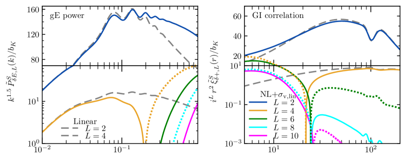
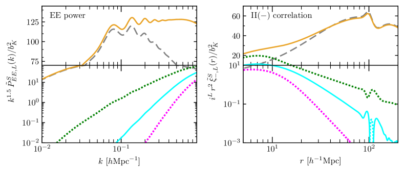
Figure 1: Multipoles of IA statistics expanded in terms of the associated Legendre polynomials, the cross power spectra between matter density and halo E-mode ellipticity $\widetilde{P}_{\delta E,L}^{S}$ (upper left), auto power spectra of halo E-mode ellipticity $\widetilde{P}_{EE,L}^{S}$ (lower left), cross correlation functions between matter density and halo ellipticity $\widetilde{\xi}_{\delta+,L}^{S}$ (upper right), and auto correlation functions of halo ellipticity $\xi_{-,\ell}^{S}$ (lower left). The prediction of linear theory is adopted for the FoG damping parameter $\sigma_{\rm v}$. The solid and dotted curves represent positive and negative values, respectively. The linear theory predictions are shown by the dashed gray curves.

Setting the angle $\phi_{\bm{r}}$ to zero, the multipole expansion of $\xi_{g+}^{S}(\bm{r})$ in Eq. (109) is analytically given by

$$\xi^{S}_{g+,0} (r)=-\sqrt{\frac{5}{12}}\,\widetilde{\xi}_{g+,2}^{S}(r)+\frac{1}{\sqrt{20}}\,\widetilde{\xi}_{g+,4}^{S}(r)$$

$$-\frac{1}{2}\sqrt{\frac{13}{210}}\,\widetilde{\xi}_{g+,6}^{S}(r)+\frac{1}{6}\sqrt{\frac{17}{70}}\,\widetilde{\xi}_{g+,8}^{S}(r)$$

$$-\frac{1}{6}\sqrt{\frac{7}{55}}\widetilde{\xi}_{g+,10}^{S}(r)+\frac{5}{\sqrt{12012}}\widetilde{\xi}_{g+,12}^{S}(r)+\cdots,$$ (113)

$$\xi^{S}_{g+,2} (r)=\sqrt{\frac{5}{12}}\,\widetilde{\xi}_{g+,2}^{S}(r)+\sqrt{\frac{5}{4}}\,\widetilde{\xi}_{g+,4}^{S}(r)$$

$$-\frac{1}{2}\sqrt{\frac{65}{42}}\,\widetilde{\xi}_{g+,6}^{S}(r)+\frac{1}{6}\sqrt{\frac{85}{14}}\,\widetilde{\xi}_{g+,8}^{S}(r)$$

$$-\frac{1}{6}\sqrt{\frac{35}{11}}\widetilde{\xi}_{g+,10}^{S}(r)+\frac{25}{\sqrt{12012}}\widetilde{\xi}_{g+,12}^{S}(r)+\cdots,$$ (114)

$$\xi^{S}_{g+,4} (r)=-\frac{3}{\sqrt{5}}\,\widetilde{\xi}_{g+,4}^{S}(r)-\frac{3}{2}\sqrt{\frac{39}{70}}\,\widetilde{\xi}_{g+,6}^{S}(r)$$

$$+\frac{3}{2}\sqrt{\frac{17}{70}}\,\widetilde{\xi}_{g+,8}^{S}(r)-3\sqrt{\frac{7}{220}}\widetilde{\xi}_{g+,10}^{S}(r)$$

$$+15\sqrt{\frac{3}{4004}}\widetilde{\xi}_{g+,12}^{S}(r)+\cdots,$$ (115)

and that of $\xi_{-}^{S}(\bm{r})$ in Eq. (110) is given by

$$\xi^{S}_{-,0}(r)= \sqrt{\frac{7}{20}}\widetilde{\xi}_{-,4}^{S}(r)-\frac{1}{5}\sqrt{\frac{13}{7}}\widetilde{\xi}_{-,6}^{S}(r)$$

$$+\frac{1}{15}\sqrt{\frac{187}{28}}\widetilde{\xi}_{-,8}^{S}(r)-\frac{2}{3}\sqrt{\frac{13}{385}}\widetilde{\xi}_{-,10}^{S}(r)$$

$$+\frac{25}{6\sqrt{2002}}\widetilde{\xi}_{-,12}^{S}(r)+\cdots\,,$$ (116)

$$\xi^{S}_{-,2}(r)= -\sqrt{\frac{5}{7}}\widetilde{\xi}_{-,4}^{S}(r)-\sqrt{\frac{13}{28}}\widetilde{\xi}_{-,6}^{S}(r)$$

$$+\frac{4}{3}\sqrt{\frac{34}{154}}\widetilde{\xi}_{-,8}^{S}(r)-\frac{43}{3}\sqrt{\frac{5}{4004}}\widetilde{\xi}_{-,10}^{S}(r)$$

$$+\frac{5}{3}\sqrt{\frac{11}{182}}\widetilde{\xi}_{-,12}^{S}(r)+\cdots\,,$$ (117)

$$\xi^{S}_{-,4}(r)= \frac{3}{\sqrt{140}}\widetilde{\xi}_{-,4}^{S}(r)+\frac{6}{5}\sqrt{\frac{13}{7}}\widetilde{\xi}_{-,6}^{S}(r)$$

$$+\frac{3}{5}\sqrt{\frac{17}{308}}\widetilde{\xi}_{-,8}^{S}(r)-3\sqrt{\frac{11}{455}}\widetilde{\xi}_{-,10}^{S}(r)$$

$$+\frac{45}{2\sqrt{2002}}\widetilde{\xi}_{-,12}^{S}(r)+\cdots\,.$$ (118)

Each multipole moment of the GI and II($-$) correlation functions involving the nonlinear RSD damping factor is expressed by infinite terms in the standard Legendre basis, unlike in the associated Legendre basis (see Eqs. (111) and (112)). These are the equations used to extract cosmological information from the IA statistics of the SDSS galaxies in Ref. Okumura and Taruya (2023).

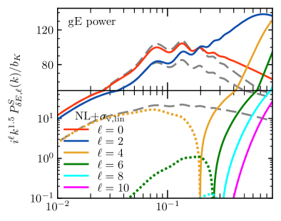
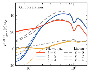
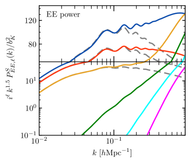
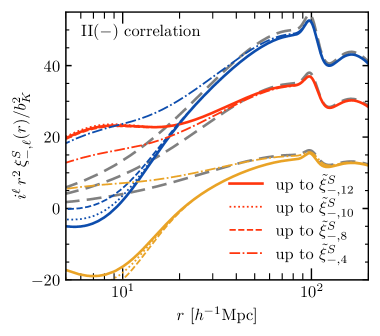
Figure 2: Similar with Fig. 1, but Multipoles of IA statistics expanded in terms of the standard Legendre polynomials. Since the models of the GI and II($-$) correlation functions of this basis are expressed by the infinite sums of those of the associated Legendre polynomials, the upper-right and lower-right panels show the results of the convergence test, the summation up to $L=4$, 8, 10 and 12 shown by the dot-dashed, short-dashed, dotted and solid curves, respectively.

V Numerical results

In this section, we present numerical results of the phenomenological model of the redshift-space IA statistics derived in the previous sections. We present the matter density–halo shape cross-correlations ($\widetilde{P}_{\delta E,L}^{S}$ and $\widetilde{\xi}_{\delta+,L}^{S}$) and halo shape auto-correlations ($\widetilde{P}_{EE,L}^{S}$ and $\widetilde{\xi}_{-,L}^{S}$) computed in the associated Legendre basis, and these in the standard Legendre basis. Since we consider for the cross correlations the matter density field, not the biased object field, we use the symbols $\widetilde{P}_{\delta E,L}^{S}$ and $\widetilde{\xi}_{\delta+,L}^{S}$, rather than $\widetilde{P}_{gE,L}^{S}$ and $\widetilde{\xi}_{g+,L}^{S}$, respectively (they are equivalent if we set $b=1$). We use the publicly-available CLASS code Blas et al. (2011) to compute the linear matter power spectrum $P_{\delta\delta}(k)$, and adopt the revised Halofit model to obtain the nonlinear correction (Takahashi et al., 2012). We then use the fitting formulae derived by Hahn et al. (2015) to obtain $P_{\delta\theta}(k)$ and $P_{\theta\theta}(k)$.

The function $D_{\rm FoG}$ is a damping function due to the nonlinear RSD effect characterized by the one-dimensional velocity dispersion, $\sigma_{\rm v}$. We use the linear theory prediction for $\sigma_{\rm v}$, as

$$\sigma_{\rm v,lin}^{2}=\frac{1}{3}\int\frac{d^{3}\mathbf{q}}{(2\pi)^{3}}\frac{P_{\theta\theta}(q)}{q^{2}}.$$ (119)

The density–E-mode cross-power spectra $\widetilde{P}_{\delta E,L}^{S}(k)$ and E-mode auto-power spectra $\widetilde{P}_{EE,L}^{S}(k)$ computed in the associated Legendre basis, are shown in the upper-left and lower-left panels of Fig. 1, respectively. Since they are respectively scaled by $b_{K}$ and $b_{K}^{2}$, only the free parameter for these statistics is $\sigma_{\rm v}$ for which we adopt the linear theory prediction, $\sigma_{\rm v,lin}$ (Eq. 119). For $\widetilde{P}_{\delta E,L}^{S}$, only the $L=2$ and $L=4$ spectra have linear-order contributions, as shown by the gray dashed curves where we set $\sigma_{\rm v}=0$ and $P_{\delta\delta}=P_{\delta\theta}=P_{\theta\theta}$. The effect of the nonlinear RSD damping appears prominently in the $L=4$ multipole. Since the multipoles with $L\geq 6$ do not contain the linear-order contributions, they become non-zero only at small and hence nonlinear scales. The FoG effect does not have significant contributions to the E-mode auto power, $\widetilde{P}_{EE,L}^{S}(k)$, than to the cross power.

The corresponding configuration-space statistics, GI and II($-$) correlation functions, are respectively shown in the upper-right and lower-right panels of Fig. 1. The overall trend is the same as the case for the power spectra. Once again, the nonlinear RSD effect does not impact the quadrupole moment but the hexadecapole in the associated Legendre basis, $\widetilde{\xi}_{\delta+,4}^{S}$.

The multipoles of the E-mode cross- and auto-power spectra expanded in the standard Legendre basis, $P_{\delta E,\ell}^{S}(k)$ and $P_{EE,\ell}^{S}(k)$, are respectively shown in the upper-left and lower-left panels of Fig. 2. Unlike $\widetilde{P}_{\delta E,L}^{S}$, the nonlinear RSD effect contributes significantly to not only the hexadecapole but also the quadrupole for $P_{\delta E,\ell}^{S}$.

The GI and II($-$) correlation functions expanded in the standard Legendre basis are shown in the upper-right and lower-right panels of Fig. 2, respectively. Unlike the other statistics we discussed above, the nonlinear RSD model of the GI and II($-$) correlation functions expanded by the standard Legendre polynomials have infinite terms as we saw in Sec. IV.2. The figure demonstrates that adding the terms up to $\widetilde{\xi}_{X,L}^{S}$ with $L=12$ makes the multipoles $\xi_{X,\ell}^{S}$ ($\ell=0,2,4$) converged even at small scales of interest. As is the case with the power spectra, while the nonlinear RSD effect in the GI correlation functions is prominent in the hexadecapole in the associated Legendre basis, it is in the quadrupole in the standard Legendre basis. However, the nonlinear RSD effect contributes to the gE power spectrum and GI correlation function quite differently in the standard Legendre basis.

VI Comparison to $N$-body simulations

VI.1 $N$-body simulations and Subhalo catalogs

As in a series of our papers (Okumura et al., 2017, 2018, 2019, 2020), we use $N$-body simulations run as a part of the DARK QUEST project (Nishimichi et al., 2019). We employ $n_{p}=2048^{3}$ particles of mass $m_{p}=8.15875\times 10^{10}{\hbox{$~{}h^{-1}$}{M_{\odot}}}$ in a cubic box of side $L_{\rm box}=2{\hbox{$~{}h^{-1}$}{\rm~{}Gpc}}$. In total, we have the data set from eight independent realizations and we specifically analyze the snapshots at $z=0.306$.

Halos are identified using the ROCKSTAR algorithm (Behroozi et al., 2013). Their velocities and positions are determined by the average of the member particles within the innermost 10% of the subhalo radius. The halo mass is defined by a sphere with a radius $R_{\rm 200m}$ within which the enclosed average density is 200 times the mean matter density, as $M_{h}\equiv M_{\rm 200m}$. We create two halo catalogs, one with $M_{h}\geq 10^{13}h^{-1}M_{\odot}$ and another with $M_{h}\geq 10^{14}h^{-1}M_{\odot}$, referred to as “groups” and “clusters”. Note that we remove subhalos, whose center is included within the sphere of $R_{\rm 200m}$ of a more massive neighbor, from these samples. To see the effect of the satellite galaxies on the IA statistics, we also create mock galaxy catalogs using a halo occupation distribution (HOD) model Zheng et al. (2005) applied for the LOWZ galaxy sample of the SDSS-III Baryon Oscillation Spectroscopic Survey obtained by Ref. Parejko et al. (2013). We populate (sub)halos with galaxies according to the best-fitting HOD $N(M_{h})$. After assigning a central galaxy at the center of a host halo, we randomly draw $N(M_{h})-1$ member subhalos within its $R_{\rm 200m}$ to mimic the positions and velocities of the satellites. We use a random selection of subhalos rather than the largest subhalos because a satellite subhalo undergoes tidal disruption in the host halo and its mass decreases as it goes toward the center of the gravitational potential. We call this subhalo catalog “HOD luminous red galaxies (LRGs)”. Properties of the three subhalo samples constructed above are summarized in Table 3.

Due to the limited hard disk space, the information of dark matter particles could have been stored partially and thus was lost for four realizations out of eight. Hence, we could not measure some of the statistics for which the information of dark matter particles is needed, while the information of the halos including the direction of the major axis traced by the dark matter particles was available for all eight realizations. Thus, when the presented statistics include the density field of dark matter in the following analysis, the result is obtained from four realizations; otherwise it is out of the entire eight realizations.

We assume subhalos to have triaxial shapes (Jing and Suto, 2002) and estimate the orientations of their major axes using the second moments of the distribution of member particles projected onto the celestial plane. The two-component ellipticity of galaxies is defined as

$$\gamma_{(+,\times)}(\bm{x})=\frac{1-q^{2}}{1+q^{2}}\left(\cos{(2\phi_{x})},\sin{(2\phi_{x})}\right),$$ (120)

where $\phi_{x}$ is the position angle of the major axis relative to the reference axis, defined on the plane normal to the line-of-sight direction, and $q$ is the minor-to-major axis ratio of a galaxy shape. We set $q$ to zero for simplicity Okumura et al. (2009); Okumura and Jing (2009).

Table 3: Properties of mock subhalo samples at $z=0.306$. The quantity $f_{\rm sat}$ is the number fraction of satellite subhalos, $M_{\mathrm{min}}$ and $\overline{M}$ are the minimum and average halo mass, respectively, $\overline{n}$ is the number density, and $b$ and $b_{K}$ are respectively the halo density and shape biases computed in the large-scale limit.

Types	$f_{\rm sat}$	$10^{-12}M_{\rm min}$	$10^{4}\overline{n}$	$b$	$b_{K}$	$10^{-12}\overline{M}$
$[h^{-1}M_{\odot}]$		$[h^{3}{\rm~{}Mpc}^{-3}]$	$[h^{-1}M_{\odot}]$
Groups	0	10	$4.34$	$1.65$	$0.54$	32.2
Clusters	0	100	$0.205$	$3.11$	0.86	188
HOD	0.137	1.63	$5.27$	$1.70$	0.47	25.2
LRGs

VI.2 Estimators

Here, we present estimators to measure from $N$-body simulations the power spectra and correlation functions of intrinsic halo shapes in redshift space.

VI.2.1 Power spectra

Multipole moments of the three-dimensional power spectra of the E-mode field of halo shapes with the matter/halo distribution, $P_{gE,\ell}^{S}(k)$, and of the auto-power spectra of the E-mode field, $P_{EE,\ell}^{S}(k)$, have been measured in the Legendre basis from simulations in Refs. Kurita et al. (2021); Shi et al. (2021). These measurements have been extended to the multipole moments expanded in the associated Legendre basis in Ref. Kurita and Takada (2022), $\widetilde{P}_{gE,L}^{S}(k)$ and $\widetilde{P}_{EE,L}^{S}(k)$, respectively.

The density and E-mode shape fields are obtained by assigning the mass/ellipticity elements of subhalos to a $1024^{3}$ uniform Cartesian mesh using the Cloud-In-Cell (CIC) scheme. We then apply the fast Fourier transform to estimate the density and E-mode auto-power spectra, $P_{gg}(\bm{k})$ and $P_{EE}(\bm{k})$, respectively, and their cross power spectrum $P_{gE}(\bm{k})$. Note that we employ the interlacing technique to reduce the aliasing effect in addition to the deconvolution of the CIC kernel in Fourier space (Sefusatti et al., 2016). The measured auto-power spectra are affected by the shot noise. The Poisson distribution is assumed to estimate the shot noise for $P_{gg}^{S}$ and it is subtracted from the monopole moment in the standard Legendre basis, $P_{gg,0}(k)$. To estimate the shot noise for the E-mode auto-power spectrum, $P_{EE}^{S}$, we measure the B-mode auto-power spectrum, $P_{BB}^{S}$, and subtract its constant value at the large-scale limit from $P_{EE}^{S}$ to take the non-Poisson shot noise into account (Kurita et al., 2021). Note that even the Poisson shot noise is not orthogonal to any multipole expanded in terms of the associated Legendre polynomials, unlike the case of the standard Legendre polynomials [$\int^{1}_{-1}d\mu\mathcal{L}_{\ell}(\mu)=2\delta_{0\ell}$]. Thus, the B-mode auto-power spectra in the associated Legendre basis, $\widetilde{P}_{BB,L}^{S}$, need to be subtracted from $\widetilde{P}_{EE,L}^{S}$ with $L$ being arbitrary.

VI.2.2 Correlation functions

Multipole moments of the correlation functions of galaxy/halo shape fields have been measured by Refs. Singh and Mandelbaum (2016); Okumura et al. (2020). We use estimators for the multipole correlation functions proposed in Ref. Okumura et al. (2020), $\xi_{X,\ell}^{S}(r)$ ($X=\{g+,+,-\}$), expressed as

$$\xi_{X,\ell}^{S}(r)=\frac{2\ell+1}{2}\frac{1}{RR(r)}\sum\limits_{j,k|r=|\bm{r}_{jk}|}W_{X,jk}\mathcal{L}_{\ell}(\mu_{jk}),$$ (121)

where $\bm{r}_{jk}=\bm{s}_{k}-\bm{s}_{j}$ with $\bm{s}_{j}$ the redshift-space position of $j$-th halo, $\mu_{jk}=\hat{\bm{r}}_{jk}\cdot\hat{\bm{z}}$, and $RR$ is the pair counts from the random distribution, which can be analytically computed because we place the periodic boundary condition on the simulation box. For the GI and II correlation functions, $W_{g+,jk}=\gamma_{+}(\bm{s}_{j})$ and $W_{\pm,jk}=\gamma_{+}(\bm{s}_{j})\gamma_{+}(\bm{s}_{k})\pm\gamma_{\times}(\bm{s}_{j})\gamma_{\times}(\bm{s}_{k})$, respectively, where $\gamma_{(+,\times)}$ is redefined relative to the separation vector $\bm{r}_{jk}$ projected on the celestial sphere.

By analogy with Eq. (121), the multipoles of the GI and II($-$) correlation functions expanded in terms of the associated Legendre polynomials are estimated as

$$\widetilde{\xi}_{X,L}^{S}(r)= \frac{1}{RR(r)}\sum\limits_{j,k|r=|\bm{r}_{jk}|}W_{X,jk}\Theta_{L}^{m}(\mu_{jk}),$$ (122)

where $X=\{g+,-\}$ and $m=2,4$, respectively.

VI.3 Determining density and shape bias parameters

The linear density field in redshift space contains $b$ and $f$ as parameters, while the linear ellipticity field $b_{K}$. The nonlinear RSD induces the Finger-of-God type damping parameter, $\sigma_{\rm v}$, to both of the fields. We thus have four parameters, $(f,b,b_{K},\sigma_{\rm v})$, with $f$ being a cosmologically-important parameter and the others nuisance parameters.

Let us determine the bias parameters, $b$ and $b_{K}$, using the real-space statistics. The density bias parameter can be determined by the matter-halo cross- or halo auto-power spectra,

$$b(k)=\frac{P_{\delta g}(k)}{P_{\delta\delta}(k)},\qquad b(k)=\left[\frac{P_{gg}(k)}{P_{\delta\delta}(k)}\right]^{\frac{1}{2}}.$$ (123)

The parameter can be similarly determined by the corresponding configuration-space statistics,

$$b(r)=\frac{\xi_{\delta g}(r)}{\xi_{\delta\delta}(r)},\qquad b(r)=\left[\frac{\xi_{gg}(r)}{\xi_{\delta\delta}(r)}\right]^{\frac{1}{2}}.$$ (124)

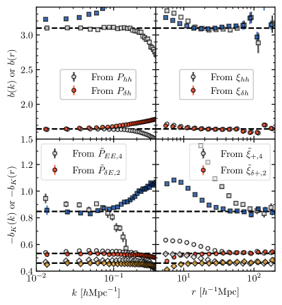
Figure 3: Halo density (upper-left) and shape (lower-left) biases determined in Fourier space. The right panes are the same as the left ones but the biases determined in configuration space. The full and open points are the biases from the cross correlations with the matter field and auto correlation with the halo field, respectively. The blue, red and yellow points are the results for clusters, groups and HOD LRGs, respectively. Since the groups and HOD LRGs have very similar density bias parameters, we do not show the results for HOD LRGs in the upper panels for clarity.

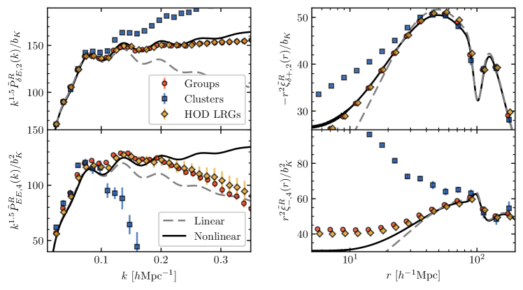
Figure 4: (Left set) IA statistics in real space, the quadrupole moment of the matter density - E-mode cross power spectrum (upper left), the quadrupole moment of the matter density - shape cross correlation function (upper right), the hexadecapole moment of the halo E-mode auto power spectrum (lower left), and the hexadecapole moment of the halo shape auto correlation function (lower right). The solid and dashed curves are the predictions of NLA and LA models, respectively.

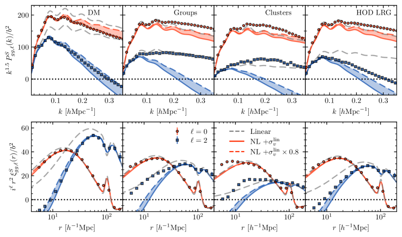
Figure 5: Redshift-space GG power spectra (upper set) and correlation functions (lower set). From the left to right, we show the results for dark matter, groups, clusters and HOD LRGs. The red and blue points are the measurements of the monopole and quadrupole moments, respectively. The solid curves are the nonlinear RSD model with the velocity dispersion predicted by linear theory, $\sigma_{\rm v}^{\rm lin}$. The shaded regions indicate the model with the values of $\sigma_{\rm v}$ of $0.8\times\sigma_{\rm v,lin}\leq\sigma_{\rm v}\leq\sigma_{\rm v,lin}$. The dashed gray curves are the linear theory prediction.

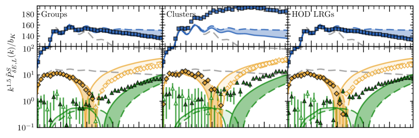
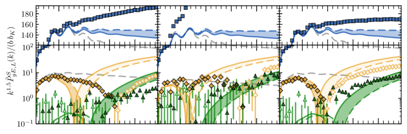
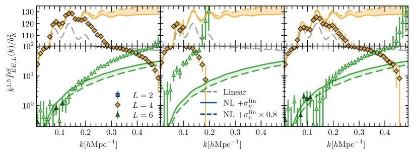
Figure 6: Multipoles of redshift-space IA power spectra expanded in terms of associated Legendre polynomials: gE power between matter density and halo E-mode ellipticity $\widetilde{P}_{\delta E,L}^{S}$ (first row), gE power between halo density and halo E-mode ellipticity $\widetilde{P}_{gE,L}^{S}$ (second row), and EE power of halo E-mode ellipticity $\widetilde{P}_{EE,L}^{S}$ (third row). The solid curves are the nonlinear RSD model with the velocity dispersion predicted by linear theory, $\sigma_{\rm v,lin}$. The shaded regions indicate the model with the values of $\sigma_{\rm v}$ of $0.8\sigma_{\rm v,lin}\leq\sigma_{\rm v}\leq\sigma_{\rm v,lin}$. Linear theory predictions for the multipoles $\widetilde{P}_{X,L}^{S}$ with $L\leq 4$ are shown by the gray curves.

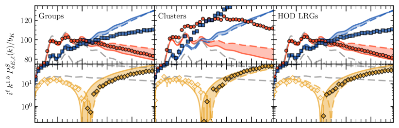
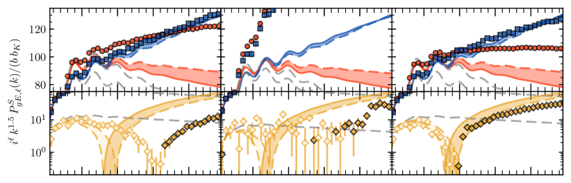
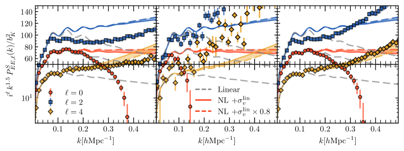
Figure 7: Similar to Fig. 6 but multipoles of redshift-space IA power spectra expanded in terms of standard Legendre polynomials: gE power between matter density and halo E-mode ellipticity $P_{\delta E,\ell}^{S}$ (first row), gE power between halo density and halo E-mode ellipticity $P_{gE,\ell}^{S}$ (second row), and EE power of halo E-mode ellipticity $P_{EE,\ell}^{S}$ (third row).

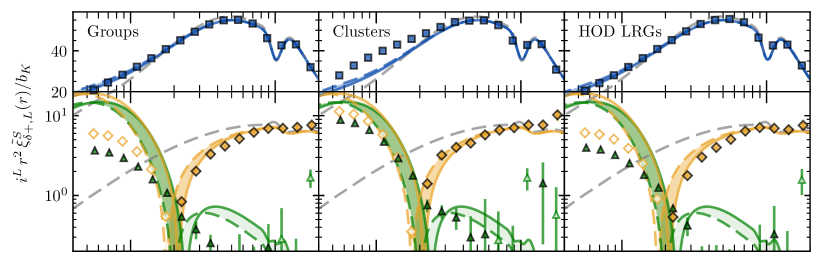
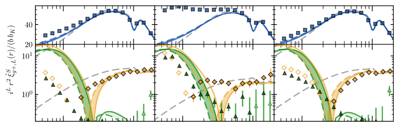
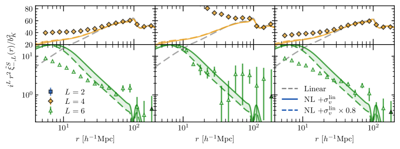
Figure 8: Similar to Fig. 6 but for multipoles of redshift-space IA correlation functions expanded in terms of associated Legendre polynomials: GI correlation between matter density and halo ellipticity $\widetilde{\xi}_{\delta+,L}^{S}$ (first row), GI correlation between halo density and ellipticity $\widetilde{\xi}_{g+,L}^{S}$ (second row), and II($-$) correlation of halo ellipticity $\widetilde{\xi}_{-,L}^{S}$ (third row).

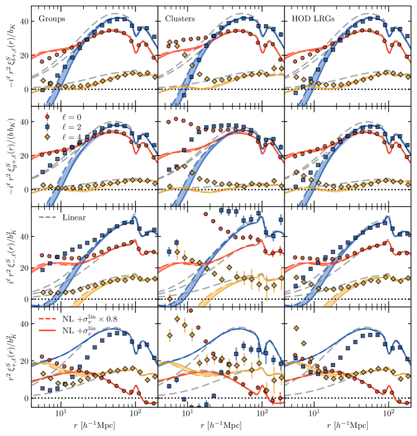
Figure 9: Similar to Fig. 8 but for multipoles of redshift-space IA correlation functions expanded in terms of standard Legendre polynomials: GI correlation between matter density and halo ellipticity $\xi_{\delta+,\ell}^{S}$ (first row), GI correlation between halo density and ellipticity $\xi_{g+,\ell}^{S}$ (second row), and II($\mp$) correlations of halo ellipticity $\xi_{\mp,\ell}^{S}$ (third and fourth rows). Our model of the GI and II($-$) correlation functions in the standard Legendre basis contains infinite series of terms, and here we show the modeling results summed up to the twelfth order (see the text).

The values of $b_{K}$ for our halo samples had already been determined in Refs. Okumura et al. (2019, 2020). Here we re-measure them using the correlators of the halo ellipticity field expanded in the associated Legendre basis. In Fourier space, using the cross-power spectra of the matter density and halo E-mode and the auto-power spectra of the halo E-mode, respectively, the shape bias is measured as

$$b_{K}(k) =-\frac{\sqrt{15}}{4}\frac{\widetilde{P}_{\delta E,2}(k)}{P_{\delta\delta}(k)},$$ (125)

$$b_{K}(k) =-\left[\frac{\sqrt{35}}{5}\frac{\widetilde{P}_{EE,4}(k)}{P_{\delta\delta}(k)}\right]^{\frac{1}{2}}.$$ (126)

Similarly in configuration space, using the cross- and auto-correlation functions, the shape bias is respectively estimated as

$$b_{K}(r) =\frac{\sqrt{15}}{4}\frac{\widetilde{\xi}_{\delta+,2}(r)}{\xi_{\delta\delta,2}(r)},$$ (127)

$$b_{K}(r) =-\left[\frac{3\sqrt{35}}{16}\frac{\widetilde{\xi}_{-,4}(r)}{\xi_{\delta\delta,4}(r)}\right]^{\frac{1}{2}},$$ (128)

where unlike the multipoles $\widetilde{\xi}_{\delta+,2}(r)$ and $\widetilde{\xi}_{-,4}(r)$, $\xi_{\delta\delta}(r)$ is isotropic and $\xi_{\delta\delta,\ell}(r)$ is the Hankel transform of $P_{\delta\delta}(k)$, $\xi_{\delta\delta,\ell}(r)=\mathcal{H}_{\ell}^{-1}[P_{\delta\delta}(k)](r)$ [Eq. (61)]. Since $\xi_{\delta\delta,\ell}(r)$ with $\ell\neq 0$ cannot be measured from simulations directly in configuration space, we compute them from the nonlinear matter power spectra $P_{\delta\delta}(k)$.

Fig. 3 shows the halo biases defined above and determined from simulations. The density bias parameters, $b$, are shown in the upper panels. The shot noise was corrected for the bias determined from the auto-power spectrum assuming the Poisson distribution, and thus suppressed at high-$k$. On the other hand the bias obtained from the cross-power spectrum tends to have larger values at high-$k$, particularly for more massive halos. They are common features seen in earlier studies (e.g., Okumura et al. (2012b)). The density bias parameters determined from cross- and auto-correlation functions in configuration space behave similarly. We use the large-scale limits of the $b(k)$ and $b(r)$ values to determine the linear bias. The resultant bias values are shown in Table 3.

The measured shape bias parameters, $b_{K}$, are shown in the lower panels of Fig. 3. The shape bias parameters from auto- and cross-power spectra, $\widetilde{P}_{EE,4}$ and $\widetilde{P}_{\delta E,2}$, respectively, behave very similarly, except for the massive halos. The shape field is more affected by the non-Poisson shot noise than the density field Kurita et al. (2021), and it cannot be properly subtracted even though we use the large-scale limit of $\widetilde{P}_{BB,4}$. The shape bias parameters determined from the cross-power spectra are well consistent with those from both the auto- and cross-correlation functions, $\widetilde{\xi}_{+,4}$ and $\widetilde{\xi}_{g+,2}$, respectively. The parameter determined from $\widetilde{\xi}_{+,4}$ starts to deviate from the constant at larger scales than that from $\widetilde{\xi}_{\delta+,2}$, since the shape field is density-weighted and thus the shape auto-correlation is more severely affected by it. The linear shape bias parameters constrained by the large-scale values of $b_{K}(k)$ and $b_{K}(r)$ are also shown in Table 3. It is interesting to note that the HOD LRG sample has a lower $b_{K}$ value than the group sample though they have similar density bias $b$ values. It is because the existence of satellite galaxies/subhalos tends to increase the density bias $b$ but decrease the shape bias $b_{K}$ due to the misalignment between the major axes of satellites and their host halos.

The left panels of Fig. 4 show the cross- and auto-power spectra of the shape field in real space, $\widetilde{P}_{\delta E,2}$ and $\widetilde{P}_{EE,4}$, respectively. The right panels of Fig. 4 are similar to the left panels but show the cross- and auto-correlation functions of the shape field, $\widetilde{\xi}_{\delta+,2}$ and $\widetilde{\xi}_{-,4}$, respectively. Both in Fourier space and configuration space, the cross- and auto-correlations are divided by $b_{K}$ and $b_{K}^{2}$ obtained above, respectively in the figure. Except for the case of the clusters, both the real-space cross-power spectra and cross-correlation functions between the matter density and halo shape fields are well described by NLA model predictions with the linear shape bias. Similar results are obtained for the shape auto-power spectra and auto-correlation functions, but discrepancies with the model predictions start to appear at larger scales.

VI.4 Model comparison with $N$-body results

Using the bias parameters, $b$ and $b_{K}$, determined in the previous subsection, here we compare our model predictions of galaxy ellipticity correlations in redshift space with $N$-body measurements. There is another nuisance parameter, the velocity dispersion parameter $\sigma_{\rm v}$. The best-fitting parameter of $\sigma_{\rm v}$ strongly depends on RSD models selected as well as the choice of the biased density field Nishimichi and Taruya (2011): The value slightly larger and smaller than the linear theory prediction, $\sigma_{\rm v,lin}$, is preferred for the dark matter and biased objects, respectively. The deviation of the best-fitting value from $\sigma_{\rm v,lin}$ gets larger for incorrect models of RSD and a broader fitting range, as indicated by a higher value of $k_{\rm max}$. In the following, we thus do not fit the $\sigma_{\rm v}$ value with $N$-body results but rather conservatively show the results for a range of $0.8\times\sigma_{\rm v,lin}\leq\sigma_{\rm v}\leq\sigma_{\rm v,lin}$ to indicate the typical level of theoretical uncertainties due to the FoG effect. Fig. 5 shows the comparison of the nonlinear model predictions for the redshift-space power spectra, $P_{gg,\ell}^{S}$, and correlation functions, $\xi_{gg,\ell}^{S}$, with the measurements from $N$-body simulations. The redshift-space power spectrum and correlation function for dark matter are well predicted by the RSD model with the damping factor with $\sigma_{\rm v,lin}$. Since the group and cluster samples do not contain subhalos, the measurements are consistent with the linear Kaiser model but not with the nonlinear RSD model with the damping function, as expected.

Figs. 6 – 9 provide comparisons of our nonlinear RSD model predictions of IA statistics to the $N$-body results. In these figures results are shown for the group, cluster and HOD LRG samples from left to right, respectively. Figs. 6 and Figs. 7 show the results for the power spectra of the halo shape field expanded in terms of the associated and standard Legendre polynomials, respectively. Figs. 8 and 9 are similar with Figs. 6 and 8, respectively, but show the results for the Fourier-counterparts, correlation functions. We will discuss in detail the results in the rest of this subsection.

VI.4.1 IA power spectra

The first row of Fig. 6 shows the cross-power spectra of matter density and halo E-mode fields, $\widetilde{P}_{\delta E,L}^{S}(k)$. The ratio $\widetilde{P}_{\delta E,L}^{S}(k)/b_{K}$ does not depend on the bias parameters, $b$ and $b_{K}$. We thus show measured $\widetilde{P}_{\delta E,L}^{S}$ divided by the best-fitting value of $b_{K}$ determined in Sec. VI.3. The measured quadrupole moments $\widetilde{P}_{\delta E,2}^{S}$, the lowest-order multipoles, are well predicted for groups and HOD LRGs by our nonlinear RSD model with the velocity dispersion predicted by linear theory, $\sigma_{\rm v,lin}$. On the other hand, there is a large discrepancy for clusters at $k>0.1{\hbox{$~{}h{\rm~{}Mpc}^{-1}$}}$. Interestingly, our model for the hexadecapole moment, $\widetilde{P}_{\delta E,4}^{S}$, well explains the measured ones not only for groups and HOD LRGs but also for clusters. The hexadecapole is severely affected by the nonlinear RSD effect, and its sign flips at around $k\sim 0.2{\hbox{$~{}h{\rm~{}Mpc}^{-1}$}}$, the scale depending on the typical value of $\sigma_{\rm v}$, and thus the LA model fails to predict the measured hexadecapole. Furthermore, our model provides qualitatively good agreement with the the fully-nonlinear, higher-order moment, $\widetilde{P}_{\delta E,6}^{S}$, measured for all the shape samples.

The second row of Fig. 6 shows the cross-power spectra of halo density and E-mode fields, $\widetilde{P}_{gE,L}^{S}$. While the overall trend is similar with $\widetilde{P}_{\delta E,L}^{S}$ in the first row, here we see the extra contribution of the halo density bias. Since we assume the simplest linear bias, the discrepancy between the model and measurement starts to appear at lower $k$, and gets more significant for more massive halos, as seen in the result for clusters (halos with masses of $M_{h}\geq 10^{14}h^{-1}M_{\odot}$ ).

The third row of Fig. 6 shows the auto-power spectra of the halo E-mode field, $\widetilde{P}_{EE,L}^{S}$. While this quantity is not affected by the halo density bias at linear order, it is by the shot noise. We measure the B-mode power spectra in the same basis, $\widetilde{P}_{BB,L}^{S}$, and subtract their large-scale limits from $\widetilde{P}_{EE,L}^{S}$. This estimation of the shot noise becomes more incorrect for more massive, thus rarer halos. Our model therefore fails to predict the measurements of $\widetilde{P}_{EE,4}$ at $k>0.1{\hbox{$~{}h^{-1}$}{\rm~{}Mpc}}$ and $\widetilde{P}_{EE,6}$ at all the scales for clusters. On the other hand, the model works reasonably well at $k<0.2{\hbox{$~{}h^{-1}$}{\rm~{}Mpc}}$ for less massive halos, namely groups and HOD LRGs.

As seen in Fig. 7, the agreement between the models and measurements of the IA power spectra expanded in terms of the standard Legendre polynomials is similar with that in Fig. 6. It is expected because they are equivalent quantities but expanded by the different basis. However, unlike the EE power spectrum in the associated Legendre basis, $\widetilde{P}_{EE,L}^{S}$, only the monopole of that in the standard Legendre basis, $P_{EE,0}^{S}$, is affected by the shot noise and thus suppressed significantly at high-$k$ due to the non-Poissonian shot noise contribution. It is interesting to note that $P_{EE,\ell}^{S}$ ($\ell=0,2,4$) are noisier than $\widetilde{P}_{EE,4}^{S}$ because the linear information encoded in the latter is split into the three multipoles in the standard Legendre basis.

VI.4.2 IA correlation functions

Fig. 8 shows the results similar to Fig. 6 but for the correlation functions. The first, second and third rows are respectively multipoles of the GI correlation for matter density and halo shape fields, $\widetilde{\xi}_{\delta+,L}^{S}$, GI correlation for halo density and halo shape fields, $\widetilde{\xi}_{g+,L}^{S}$, and II($-$) auto-correlation for halo shape field, $\widetilde{\xi}_{-,L}^{S}$, expanded in the associated Legendre basis. The comparison of our model predictions to the $N$-body measurements shows a very similar tendency with the Fourier-space results: the measurements of $\widetilde{\xi}_{\delta+,L}^{S}$ are in good agreement with our models, and the agreement gets worse for $\widetilde{\xi}_{g+,L}^{S}$, particularly for the cluster shape field. One exception is that the auto-correlation in configuration space is not affected by the shot noise as severely as in Fourier space. Thus, one can see a reasonable agreement between the predictions and measurements for $\widetilde{\xi}_{-,L}^{S}$, and even the hexadecapole of clusters is correctly predicted at the large-scale limit, unlike $\widetilde{P}_{EE,4}$.

Unlike the power spectra, the nonlinear redshift-space correlation functions expanded in terms of the standard Legendre polynomials behave differently from those of the associated Legendre polynomials, as shown in Fig. 9. Our nonlinear RSD model of the GI and II($-$) correlation functions expanded in terms of the standard Legendre polynomials contains infinite series of the associated Legendre polynomials. As shown in Fig. 2, the model converges by adding the term up to sufficiently higher-order. We computed the expansion up to the twelfth order and confirmed the convergence of the formula. We thus show the modeling results summed up to the twelfth order. The first row shows the GI correlation functions between matter density and halo shape fields, $\xi_{\delta+,\ell}^{S}$. The results for the quadrupole moments for all the halo samples are well explained by our nonlinear RSD model. The second row shows the GI correlation functions between halo density and shape fields, $\xi_{g+,\ell}^{S}$. Agreement between the predictions and measurements gets worse than the case of $\xi_{\delta+,\ell}^{S}$, due to the nonlinear density bias effect. The third and fourth rows show the II($\mp$) correlation functions, $\xi_{-,\ell}^{S}$ and $\xi_{+,\ell}^{S}$, respectively. The standard Legendre coefficients of the II($-$) correlations, $\xi_{-,\ell}^{S}$, are noisier than the associated Legendre coefficients, $\widetilde{\xi}_{-,L}^{S}$, since for the latter the linear contribution is compressed to only one, hexadecapole moment $\widetilde{\xi}_{-,L}^{S}$. The model constructed for the HOD LRG sample is very close to the one used to constrain the growth rate from the SDSS survey in Ref. Okumura and Taruya (2023).

VII Conclusions

In this paper, we have presented analytic model for nonlinear correlators of galaxy ellipticities in redshift space. Adopting a simple Gaussian damping function to describe the nonlinear RSD effect, known as the Finger-of-God, we have derived formulas for the multipole moments of the power spectra of galaxy ellipticity field in redshift space, expanded in not only the associated Legendre basis, a natural basis for the projected galaxy shape field, but also the standard Legendre basis, conventionally used in literature. The model had been derived for the redshift-space galaxy power spectra by Ref. Scoccimarro (2004); Taruya et al. (2010), and our model for the intrinsic alignment (IA) statistics have been derived by analogy with it. The multipoles of the correlation functions of the galaxy shape field are expressed simply by a Hankel transform of those of the power spectra.

We compared our model with the IA statistics for halos and mock galaxies measured from $N$-body simulations. The measured statistics were found to be in a better agreement with our nonlinear RSD model than the existing linear alignment model. It is the first test for the accuracy of nonlinear RSD models of the IA, though the model had already been used to place cosmological constraints using from the redshift-space correlation functions of the galaxy shape field measured from the Sloan Digital Sky Survey in Ref. Okumura and Taruya (2023).

A series of papers Matsubara (2022a, b, 2023) used integrated perturbation theory and presented a nonlinear model of the tidal field tensor, which naturally includes nonlinear RSD (see also Ref. Chen and Kokron (2023)). However, the models had not been tested against $N$-body simulation measurements. Other perturbation theory approaches, such as the TNS model Taruya et al. (2010); Nishimichi and Taruya (2011); Taruya et al. (2013) and distribution function approach Seljak and McDonald (2011); Okumura et al. (2012a, b); Vlah et al. (2012, 2013), can also be used to model the nonlinear RSD effect of galaxy shape fields. These modelings will be investigated for various halo samples and redshifts in simulations in future work.

We presented the formulas of IA statistics in redshift space expanded in terms of different bases. While they should be equivalent, the speed of the convergence at higher-order multipoles would be different (see Refs. Okumura et al. (2012a, b) for different bases for the multipole redshift-space power spectra). The investigation of this effect based on the Fisher-matrix approach will be presented in our future work.

Appendix A Higher-order multipoles

In this paper, we provided the formulas of IA statistics expanded in terms of the associated and standard Legendre polynomials and in the body text we explicitly wrote down the formulas that contain contributions of linear theory, $L\leq 4$ and $\ell\leq 4$, respectively. In this appendix, we provide our formulas for the higher-order multipoles, up to $L=12$ and $\ell=12$.

A.1 gE power spectra

The gE power spectra expanded in terms of the associated Legendre polynomials, $\widetilde{P}_{gE,L}^{S}$, are given in Eq. (44). To compute the nonlinear contributions up to $L=12$, we need to have $\mathcal{\widetilde{Q}}_{gE,L}^{(n)}$ for $4<L\leq 12$, which are given as

$$\mathcal{\widetilde{Q}}_{gE,6}^{(n)}(\alpha) =\frac{\sqrt{2730}}{64}\left[p^{(n)}(\alpha)-20p^{(n+1)}(\alpha)+70p^{(n+2)}(\alpha)-84p^{(n+3)}(\alpha)+33p^{(n+4)}(\alpha)\right],$$ (129)

$$\mathcal{\widetilde{Q}}_{gE,8}^{(n)}(\alpha) =\frac{3\sqrt{1190}}{128}\left[-p^{(n)}(\alpha)+35p^{(n+1)}(\alpha)-210p^{(n+2)}(\alpha)+462p^{(n+3)}(\alpha)\right.$$

$$\qquad\qquad\qquad\left.-429p^{(n+4)}(\alpha)+143p^{(n+5)}(\alpha)\right],$$ (130)

$$\mathcal{\widetilde{Q}}_{gE,10}^{(n)}(\alpha) =\frac{3\sqrt{385}}{512}\left[7p^{(n)}(\alpha)-378p^{(n+1)}(\alpha)+3465p^{(n+2)}(\alpha)-12012p^{(n+3)}(\alpha)\right.$$

$$\qquad\qquad\qquad\left.+19305p^{(n+4)}(\alpha)-14586p^{(n+5)}(\alpha)+4199p^{(n+6)}(\alpha)\right],$$ (131)

$$\mathcal{\widetilde{Q}}_{gE,12}^{(n)}(\alpha) =\frac{5\sqrt{3003}}{1024}\left[-3p^{(n)}(\alpha)+231p^{(n+1)}(\alpha)-3003p^{(n+2)}(\alpha)+15015p^{(n+3)}(\alpha)\right.$$

$$\qquad\qquad\qquad\left.-36465p^{(n+4)}(\alpha)+46189p^{(n+5)}(\alpha)-29393p^{(n+6)}(\alpha)+7429p^{(n+7)}(\alpha)\right].$$ (132)

Those expanded in terms of the standard Legendre polynomials, $P_{gE,\ell}^{S}$, are given in Eq. (47). To obtain the nonlinear contributions up to $\ell=12$, we need to have $\mathcal{Q}_{gE,\ell}^{(n)}$ for $4<\ell\leq 12$, which are given as

$$\mathcal{Q}_{gE,6}^{(n)}(\alpha) =-\frac{13}{32}\left[5p^{(n)}(\alpha)-110p^{(n+1)}(\alpha)+420p^{(n+2)}(\alpha)-546p^{(n+3)}(\alpha)+231p^{(n+4)}(\alpha)\right],$$ (133)

$$\mathcal{Q}_{gE,8}^{(n)}(\alpha) =\frac{17}{256}\left[35p^{(n)}(\alpha)-1295p^{(n+1)}(\alpha)+8190p^{(n+2)}(\alpha)-18942p^{(n+3)}(\alpha)\right.$$

$$\qquad\qquad\left.+18447p^{(n+4)}(\alpha)-6435p^{(n+5)}(\alpha)\right],$$ (134)

$$\mathcal{Q}_{gE,10}^{(n)}(\alpha) =\frac{21}{512}\left[-63p^{(n)}(\alpha)+3528p^{(n+1)}(\alpha)-33495p^{(n+2)}(\alpha)+120120p^{(n+3)}(\alpha)\right.$$

$$\qquad\qquad\left.-199485p^{(n+4)}(\alpha)+155584p^{(n+5)}(\alpha)-46189p^{(n+6)}(\alpha)\right],$$ (135)

$$\mathcal{Q}_{gE,12}^{(n)}(\alpha) =\frac{25}{2048}\left[231p^{(n)}(\alpha)-18249p^{(n+1)}(\alpha)+243243p^{(n+2)}(\alpha)-1246245p^{(n+3)}(\alpha)\right.$$

$$\qquad\qquad\left.+3099525p^{(n+4)}(\alpha)-4018443p^{(n+5)}(\alpha)+2615977p^{(n+6)}(\alpha)-676039p^{(n+7)}(\alpha)\right].$$ (136)

A.2 EE power spectra

Similarly to the gE power spectra, the EE spectra expanded in terms of the associated Legendre polynomials, $\widetilde{P}_{EE,L}^{S}$, are given in Eq. (51). To compute the nonlinear contributions up to $L=12$, we need to have $\mathcal{\widetilde{Q}}_{EE,L}$ for $4<L\leq 12$, which are given as

$$\mathcal{\widetilde{Q}}_{EE,6}(\alpha) =\frac{3\sqrt{91}}{32}\left[-p^{(0)}(\alpha)+15p^{(1)}(\alpha)-50p^{(2)}(\alpha)+70p^{(3)}(\alpha)-45p^{(4)}(\alpha)+11p^{(5)}(\alpha)\right],$$ (137)

$$\mathcal{\widetilde{Q}}_{EE,8}(\alpha) =\frac{3\sqrt{1309}}{128}\left[p^{(0)}(\alpha)-30p^{(1)}(\alpha)+175p^{(2)}(\alpha)-420p^{(3)}(\alpha)+495p^{(4)}(\alpha)-286p^{(5)}(\alpha)+65p^{(6)}(\alpha)\right],$$ (138)

$$\mathcal{\widetilde{Q}}_{EE,10}(\alpha) =\frac{3\sqrt{5005}}{256}\left[-p^{(0)}(\alpha)+49p^{(1)}(\alpha)-441p^{(2)}(\alpha)+1617p^{(3)}(\alpha)-3003p^{(4)}(\alpha)\right.$$

$$\qquad\qquad\qquad\left.+3003p^{(5)}(\alpha)-1547p^{(6)}(\alpha)+323p^{(7)}(\alpha)\right],$$ (139)

$$\mathcal{\widetilde{Q}}_{EE,12}(\alpha) =\frac{15\sqrt{1001}}{4096}\left[5p^{(0)}(\alpha)-360p^{(1)}(\alpha)+4620p^{(2)}(\alpha)-24024p^{(3)}(\alpha)+64350p^{(4)}(\alpha)\right.$$

$$\qquad\qquad\qquad\left.-97240p^{(5)}(\alpha)+83980p^{(6)}(\alpha)-38760p^{(7)}(\alpha)+7429p^{(8)}(\alpha)\right].$$ (140)

Those expanded in terms of the standard Legendre polynomials, $P_{EE,\ell}^{S}$, are given in Eq. (53), and $\mathcal{Q}_{EE,\ell}$ for $4<\ell\leq 12$ are given as

$$\mathcal{Q}_{EE,6}(\alpha) =\frac{13}{32}\left[-5p^{(0)}(\alpha)+115p^{(1)}(\alpha)-530p^{(2)}(\alpha)+966p^{(3)}(\alpha)-777p^{(4)}(\alpha)+231p^{(5)}(\alpha)\right],$$ (141)

$$\mathcal{Q}_{EE,8}(\alpha) =\frac{17}{256}\left[35p^{(0)}(\alpha)-1330p^{(1)}(\alpha)+9485p^{(2)}(\alpha)-27132p^{(3)}(\alpha)+37389p^{(4)}(\alpha)\right.$$

$$\qquad\qquad\left.-24882p^{(5)}(\alpha)+6435p^{(6)}(\alpha)\right],$$ (142)

$$\mathcal{Q}_{EE,10}(\alpha) =\frac{21}{512}\left[-63p^{(0)}(\alpha)+3591p^{(1)}(\alpha)-37023p^{(2)}(\alpha)+153615p^{(3)}(\alpha)-319605p^{(4)}(\alpha)\right.$$

$$\qquad\qquad\left.+355069p^{(5)}(\alpha)-201773p^{(6)}(\alpha)+46189p^{(7)}(\alpha)\right],$$ (143)

$$\mathcal{Q}_{EE,12}(\alpha) =\frac{25}{2048}\left[231p^{(0)}(\alpha)-18480p^{(1)}(\alpha)+261492p^{(2)}(\alpha)-1489488p^{(3)}(\alpha)+4345770p^{(4)}(\alpha)\right.$$

$$\qquad\qquad\left.-7117968p^{(5)}(\alpha)+6634420p^{(6)}(\alpha)-3292016p^{(7)}(\alpha)+676039p^{(8)}(\alpha)\right].$$ (144)

A.3 GI and II($-)$ power spectra

We showed the GI and II($-$) power spectra expanded in terms of the spherical harmonics, $P_{\ell,2}^{g+}$ (Eq. 96) and $P_{\ell,4}^{-}$ (Eq. 99), respectively. To compute the them with nonlinear contributions up to $\ell=12$, we need to have the terms $\mathcal{Q}_{g+,\ell}^{(n)}$ and $\mathcal{Q}_{-,\ell}$ for $4<\ell\leq 12$, which are given as

$$\mathcal{Q}_{g+,6}^{(n)}(\alpha) =\frac{2\sqrt{105}}{36465}\Bigl{(}85\sqrt{13}F_{4}^{(n)}-442F_{6}^{(n)}+11\sqrt{221}F_{8}^{(n)}\Bigr{)},$$ (145)

$$\mathcal{Q}_{g+,8}^{(n)}(\alpha) =\frac{2\sqrt{1105}}{20995}\Bigl{(}19\sqrt{7}F_{6}^{(n)}-2\sqrt{1547}F_{8}^{(n)}+\sqrt{975}F_{10}^{(n)}\Bigr{)},$$ (146)

$$\mathcal{Q}_{g+,10}^{(n)}(\alpha) =\frac{3\sqrt{110}}{260015}\left(115\sqrt{119}F_{8}^{(n)}-1190\sqrt{3}F_{10}^{(n)}+323\sqrt{7}F_{12}^{(n)}\right),$$ (147)

$$\mathcal{Q}_{g+,12}^{(n)}(\alpha) =\frac{\sqrt{286}}{90045}\Bigl{(}783F_{10}^{(n)}-290\sqrt{21}F_{12}^{(n)}+23\sqrt{609}F_{14}^{(n)}\Bigr{)},$$ (148)

and

$$\mathcal{Q}_{-,6}(\alpha) =\frac{4\sqrt{2}}{323323}\Bigl{(}323\sqrt{455}F_{2}^{(0)}-1292\sqrt{91}F_{4}^{(0)}+3458\sqrt{7}F_{6}^{(0)}-84\sqrt{1547}F_{8}^{(0)}+77\sqrt{39}F_{10}^{(0)}\Bigr{)},$$ (149)

$$\mathcal{Q}_{-,8}(\alpha) =\frac{4\sqrt{22}}{7436429}\Bigl{(}3059\sqrt{119}F_{4}^{(0)}-1932\sqrt{1547}F_{6}^{(0)}+25806\sqrt{7}F_{8}^{(0)}-4004\sqrt{51}F_{10}^{(0)}+429\sqrt{119}F_{12}^{(0)}\Bigr{)},$$ (150)

$$\mathcal{Q}_{-,10}(\alpha) =\frac{4\sqrt{110}}{48474225}\Bigl{(}30015\sqrt{7}F_{6}^{(0)}-5220\sqrt{1547}F_{8}^{(0)}+32886\sqrt{39}F_{10}^{(0)}-9860\sqrt{91}F_{12}^{(0)}+323\sqrt{2639}F_{14}^{(0)}\Bigr{)},$$ (151)

$$\mathcal{Q}_{-,12}(\alpha) =\frac{8}{420756273}\Bigl{(}24273\sqrt{17017}F_{8}^{(0)}-427924\sqrt{429}F_{10}^{(0)}+300390\sqrt{1001}F_{12}^{(0)}-27132\sqrt{29029}F_{14}^{(0)}+52003\sqrt{273}F_{16}^{(0)}\Bigr{)}.$$ (152)

To obtain then, we need to compute $F_{q}^{(n)}$ with $q\leq 16$. These quantities for $0\leq q\leq 8$ are shown in Eqs. (101) – (105). These with $8<q\leq 16$ are obtained as

$$F_{10}^{(n)}(\alpha) =\frac{A_{10}}{256}\Bigl{(}46189p^{(n+5)}-109395p^{(n+4)}+90090p^{(n+3)}-30030p^{(n+2)}+3465p^{(n+1)}-63p^{(n)}\Bigr{)},$$ (153)

$$F_{12}^{(n)}(\alpha) =\frac{A_{12}}{1024}\Bigl{(}676039p^{(n+6)}-1939938p^{(n+5)}+2078505p^{(n+4)}-1021020p^{(n+3)}+225225p^{(n+2)}$$

$$\qquad\qquad\quad-18018p^{(n+1)}+231p^{(n)}\Bigr{)},$$ (154)

$$F_{14}^{(n)}(\alpha) =\frac{A_{14}}{2048}\Bigl{(}5014575p^{(n+7)}-16900975p^{(n+6)}+22309287p^{(n+5)}-14549535p^{(n+4)}+4849845p^{(n+3)}$$

$$\qquad\qquad\quad-765765p^{(n+2)}+45045p^{(n+1)}-429p^{(n)}\Bigr{)}.$$ (155)

$$F_{16}^{(n)}(\alpha) =\frac{A_{16}}{32768}\Bigl{(}300540195p^{(n+8)}-1163381400p^{(n+7)}+1825305300p^{(n+6)}-1487285800p^{(n+5)}$$

$$\qquad\qquad\quad+669278610p^{(n+4)}-162954792p^{(n+3)}+19399380p^{(n+2)}-875160p^{(n+1)}+6435p^{(n)}\Bigr{)}.$$ (156)

As we showed in section IV.2, each multipole of the IA correlation functions in the standard Legendre basis are expressed by infinite terms expanded in terms of the associated Legendre polynomials. Computing the above quantities is necessary to obtain the converged predictions for the correlation function multipoles in the standard Legendre basis as shown in the body text.

Appendix B Linear theory limit

The model developed in this paper has a form that is a combination of the nonlinear alignment model (NLA) multiplied by the Gaussian damping function due to the nonlinear RSD effect. As introduced in Section III.2, the damping function is given by $D_{\rm FoG}(fk\mu_{\bm{k}}\sigma_{\rm v})=\exp{\left(-\alpha\mu_{\bm{k}}^{2}/2\right)}$, where $\alpha=(f\sigma_{\rm v}k)^{2}$. We can remove the effect of the nonlinear RSD by taking the $\sigma_{\rm v}\to 0$ limit. In this appendix we provide the formulas with this limit, though they were already given in our previous work Okumura and Taruya (2020); Saga et al. (2023).

Note again that the multipoles in the associated Legendre basis in this paper are expanded by the normalized associated Legendre function $\Theta_{L}^{m}$ [Eq. (43)] and thus denoted by tilde.

B.1 Power spectra

The gE power spectra expanded in terms of the associated Legendre polynomials in the linear theory limit are given by

$$\widetilde{P}_{gE,2}^{S}(k) =\frac{4}{\sqrt{15}}b_{K}\left[bP_{\delta\delta}(k)+\frac{1}{7}fP_{\delta\theta}(k)\right],$$ (157)

$$\widetilde{P}_{gE,4}^{S}(k) =\frac{8}{21\sqrt{5}}b_{K}fP_{\delta\theta}(k).$$ (158)

Those expanded in terms of the standard Legendre polynomials are by

$$P_{gE,0}^{S}(k) =\frac{2}{3}b_{K}\left[bP_{\delta\delta}(k)+\frac{1}{5}fP_{\delta\theta}(k)\right],$$ (159)

$$P_{gE,2}^{S}(k) =-\frac{2}{3}b_{K}\left[bP_{\delta\delta}(k)-\frac{1}{7}fP_{\delta\theta}(k)\right],$$ (160)

$$P_{gE,4}^{S}(k) =-\frac{8}{35}b_{K}fP_{\delta\theta}(k),$$ (161)

The EE power spectrum expanded in terms of the associated Legendre polynomials in the linear theory limit is only $\widetilde{P}_{EE,4}^{S}$, given by

$$\widetilde{P}_{EE,4}^{S}(k) =\frac{16}{3\sqrt{35}}b_{K}^{2}P_{\delta\delta}(k),$$ (162)

and those in the standard Legendre basis are by

$$P_{EE,0}^{S}(k) =\frac{8}{15}b_{K}^{2}P_{\delta\delta}(k),$$ (163)

$$P_{EE,2}^{S}(k) =-\frac{16}{21}b_{K}^{2}P_{\delta\delta}(k),$$ (164)

$$P_{EE,4}^{S}(k) =\frac{8}{35}b_{K}^{2}P_{\delta\delta}(k).$$ (165)

B.2 Correlation functions

The GI correlation functions expanded in terms of the associated Legendre polynomials $\widetilde{\xi}_{g+,L}^{S}$ in the linear theory limit ($L=2,4$) are given by

$$\widetilde{\xi}_{g+,2}^{S}(r) =-\frac{4}{7}\sqrt{\frac{1}{15}}\,b_{K}\left[7b\xi_{\delta\delta,2}(r)+f\xi_{\delta\theta,2}(r)\right]\,,$$

$$\widetilde{\xi}_{g+,4}^{S}(r) =\frac{8}{21}\sqrt{\frac{1}{5}}\,b_{K}f\,\xi_{\delta\theta,4}(r),$$ (166)

and similarly, the non-vanishing coefficient for the II($-$) correlation $\widetilde{\xi}_{-,L}^{S}$ appears only for $L=4$,

$$\widetilde{\xi}_{-,4}^{S}(r) =\frac{16}{3}\sqrt{\frac{1}{35}}\,b_{K}^{2}\,\xi_{\delta\delta,4}(r),$$ (167)

where the functions $\xi_{\delta\delta,L}$ and $\xi_{\delta\theta,L}$ are defined by $\xi_{\delta\delta,L}(r)=\mathcal{H}_{L}^{-1}[P_{\delta\delta}(k)](r)$ and $\xi_{\delta\theta,L}(r)=\mathcal{H}_{L}^{-1}[P_{\delta\theta}(k)](r)$, respectively.

Finally, those expressions in terms of the standard Legendre basis have $\ell=0,2$, and $4$ components. The multipoles of the GI correlation functions are given by

$$\xi^{S}_{g+,0}(r) =-\frac{2}{3}b_{K}b\,\xi_{\delta\delta,2}(r)$$

$$\quad+b_{K}f\Bigl{\{}-\frac{2}{21}\xi_{\delta\theta,2}(r)+\frac{4}{105}\xi_{\delta\theta,4}(r)\Bigr{\}},$$ (168)

$$\xi^{S}_{g+,2}(r) =\frac{2}{3}b_{K}b\,\xi_{\delta\delta,2}(r)$$

$$\quad+b_{K}f\Bigl{\{}\frac{2}{21}\xi_{\delta\theta,2}(r)+\frac{4}{21}\xi_{\delta\theta,4}(r)\Bigr{\}},$$ (169)

$$\xi^{S}_{g+,4}(r) =-\frac{8}{35}b_{K}f\,\xi_{\delta\delta,4}(r).$$ (170)

The II correlation functions in redshift space are equivalent with those in real space in the linear theory limit Okumura and Taruya (2020). The multipoles of the II($+$) and II($-$) correlation functions in the standard Legendre basis are respectively given by

$$\xi_{+,0}^{S}(r) =\frac{8}{15}b_{K}^{2}\,\xi_{\delta\delta,0}(r),$$ (171)

$$\xi_{+,2}^{S}(r) =\frac{16}{21}b_{K}^{2}\,\xi_{\delta\delta,2}(r),$$ (172)

$$\xi_{+,4}^{S}(r) =\frac{8}{35}b_{K}^{2}\,\xi_{\delta\delta,4}(r),$$ (173)

and

$$\xi_{-,0}^{S}(r) =\frac{8}{15}b_{K}^{2}\,\xi_{\delta\delta,4}(r),$$ (174)

$$\xi_{-,2}^{S}(r) =-\frac{16}{21}b_{K}^{2}\,\xi_{\delta\delta,4}(r),$$ (175)

$$\xi_{-,4}^{S}(r) =\frac{8}{35}b_{K}^{2}\,\xi_{\delta\delta,4}(r).$$ (176)

References

- Okumura and Taruya (2023) T. Okumura and A. Taruya, Astrophys. J. Lett. 945, L30 (2023), eprint 2301.06273.
- Heavens et al. (2000) A. Heavens, A. Refregier, and C. Heymans, Mon. Not. Roy. Astron. Soc. 319, 649 (2000), eprint astro-ph/0005269.
- Croft and Metzler (2000) R. A. C. Croft and C. A. Metzler, Astrophys. J. 545, 561 (2000), eprint astro-ph/0005384.
- Lee and Pen (2000) J. Lee and U.-L. Pen, Astrophys. J. Lett. 532, L5 (2000), eprint astro-ph/9911328.
- Pen et al. (2000) U.-L. Pen, J. Lee, and U. Seljak, Astrophys. J. Lett. 543, L107 (2000), eprint astro-ph/0006118.
- Catelan et al. (2001) P. Catelan, M. Kamionkowski, and R. D. Blandford, Mon. Not. Roy. Astron. Soc. 320, L7 (2001), eprint astro-ph/0005470.
- Crittenden et al. (2002) R. G. Crittenden, P. Natarajan, U.-L. Pen, and T. Theuns, Astrophys. J. 568, 20 (2002), eprint astro-ph/0012336.
- Jing (2002) Y. P. Jing, Mon. Not. Roy. Astron. Soc. 335, L89 (2002), eprint astro-ph/0206098.
- Hirata and Seljak (2004) C. M. Hirata and U. Seljak, Phys. Rev. D 70, 063526 (2004), eprint astro-ph/0406275.
- Heymans et al. (2004) C. Heymans, M. Brown, A. Heavens, K. Meisenheimer, A. Taylor, and C. Wolf, Mon. Not. Roy. Astron. Soc. 347, 895 (2004), eprint astro-ph/0310174.
- Mandelbaum et al. (2006) R. Mandelbaum, C. M. Hirata, M. Ishak, U. Seljak, and J. Brinkmann, Mon. Not. Roy. Astron. Soc. 367, 611 (2006), eprint astro-ph/0509026.
- Hirata et al. (2007) C. M. Hirata, R. Mandelbaum, M. Ishak, U. Seljak, R. Nichol, K. A. Pimbblet, N. P. Ross, and D. Wake, Mon. Not. Roy. Astron. Soc. 381, 1197 (2007), eprint astro-ph/0701671.
- Okumura et al. (2009) T. Okumura, Y. P. Jing, and C. Li, Astrophys. J. 694, 214 (2009), eprint 0809.3790.
- Joachimi et al. (2011) B. Joachimi, R. Mandelbaum, F. B. Abdalla, and S. L. Bridle, Astron. Astrophys. 527, A26 (2011), eprint 1008.3491.
- Li et al. (2013) C. Li, Y. P. Jing, A. Faltenbacher, and J. Wang, Astrophys. J. Lett. 770, L12 (2013), eprint 1303.1965.
- Singh et al. (2015) S. Singh, R. Mandelbaum, and S. More, Mon. Not. Roy. Astron. Soc. 450, 2195 (2015), eprint 1411.1755.
- Tonegawa et al. (2018) M. Tonegawa, T. Okumura, T. Totani, G. Dalton, K. Glazebrook, and K. Yabe, Publ. Astron. Soc. Japan 70, 41 (2018), eprint 1708.02224.
- Tonegawa and Okumura (2022) M. Tonegawa and T. Okumura, Astrophys. J. Lett. 924, L3 (2022), eprint 2109.14297.
- Troxel and Ishak (2015) M. A. Troxel and M. Ishak, Phys. Rept. 558, 1 (2015), eprint 1407.6990.
- Joachimi et al. (2015) B. Joachimi, M. Cacciato, T. D. Kitching, A. Leonard, R. Mandelbaum, B. M. Schäfer, C. Sifón, H. Hoekstra, A. Kiessling, D. Kirk, et al., Space Sci. Rev. 193, 1 (2015), eprint 1504.05456.
- Kirk et al. (2015) D. Kirk, M. L. Brown, H. Hoekstra, B. Joachimi, T. D. Kitching, R. Mandelbaum, C. Sifón, M. Cacciato, A. Choi, A. Kiessling, et al., Space Sci. Rev. 193, 139 (2015), eprint 1504.05465.
- Kiessling et al. (2015) A. Kiessling, M. Cacciato, B. Joachimi, D. Kirk, T. D. Kitching, A. Leonard, R. Mandelbaum, B. M. Schäfer, C. Sifón, M. L. Brown, et al., Space Sci. Rev. 193, 67 (2015), eprint 1504.05546.
- Lamman et al. (2023) C. Lamman, E. Tsaprazi, J. Shi, N. Niko Šarčević, S. Pyne, E. Legnani, and T. Ferreira, arXiv e-prints arXiv:2309.08605 (2023), eprint 2309.08605.
- Chisari and Dvorkin (2013) N. E. Chisari and C. Dvorkin, J. Cosmol. Astropart. Phys. 12, 029 (2013), eprint 1308.5972.
- Okumura et al. (2019) T. Okumura, A. Taruya, and T. Nishimichi, Phys. Rev. D 100, 103507 (2019).
- Taruya and Okumura (2020) A. Taruya and T. Okumura, Astrophys. J. Lett. 891, L42 (2020), eprint 2001.05962.
- Okumura and Taruya (2022) T. Okumura and A. Taruya, Phys. Rev. D 106, 043523 (2022), eprint 2110.11127.
- Chuang et al. (2022) Y.-T. Chuang, T. Okumura, and M. Shirasaki, Mon. Not. Roy. Astron. Soc. 515, 4464 (2022), eprint 2111.01417.
- Schmidt et al. (2015) F. Schmidt, N. E. Chisari, and C. Dvorkin, J. Cosmol. Astropart. Phys. 10, 032 (2015), eprint 1506.02671.
- Chisari et al. (2016) N. E. Chisari, C. Dvorkin, F. Schmidt, and D. N. Spergel, Phys. Rev. D 94, 123507 (2016), eprint 1607.05232.
- Akitsu et al. (2021a) K. Akitsu, T. Kurita, T. Nishimichi, M. Takada, and S. Tanaka, Phys. Rev. D 103, 083508 (2021a), eprint 2007.03670.
- Schmidt et al. (2014) F. Schmidt, E. Pajer, and M. Zaldarriaga, Phys. Rev. D 89, 083507 (2014), eprint 1312.5616.
- Chisari et al. (2014) N. E. Chisari, C. Dvorkin, and F. Schmidt, Phys. Rev. D 90, 043527 (2014), eprint 1406.4871.
- Biagetti and Orlando (2020) M. Biagetti and G. Orlando, J. Cosmol. Astropart. Phys. 2020, 005 (2020), eprint 2001.05930.
- Akitsu et al. (2023a) K. Akitsu, Y. Li, and T. Okumura, Phys. Rev. D 107, 063531 (2023a), eprint 2209.06226.
- Lee et al. (2023) J. Lee, S. Ryu, and M. Baldi, Astrophys. J. 945, 15 (2023), eprint 2206.03406.
- Shiraishi et al. (2023) M. Shiraishi, T. Okumura, and K. Akitsu, J. Cosmol. Astropart. Phys. 2023, 013 (2023), eprint 2303.10890.
- Zwetsloot and Chisari (2022) K. Zwetsloot and N. E. Chisari, Mon. Not. Roy. Astron. Soc. 516, 787 (2022), eprint 2208.07062.
- Saga et al. (2023) S. Saga, T. Okumura, A. Taruya, and T. Inoue, Mon. Not. Roy. Astron. Soc. 518, 4976 (2023), eprint 2207.03454.
- Kurita and Takada (2023) T. Kurita and M. Takada, arXiv e-prints arXiv:2302.02925 (2023), eprint 2302.02925.
- Xu et al. (2023) K. Xu, Y. P. Jing, G.-B. Zhao, and A. J. Cuesta, Nature Astronomy (2023), eprint 2306.09407.
- Takada et al. (2014) M. Takada, R. S. Ellis, M. Chiba, J. E. Greene, H. Aihara, N. Arimoto, K. Bundy, J. Cohen, O. Doré, G. Graves, et al., Publ. Astron. Soc. Japan 66, R1 (2014), eprint 1206.0737.
- DESI Collaboration et al. (2016) DESI Collaboration, A. Aghamousa, J. Aguilar, S. Ahlen, S. Alam, L. E. Allen, C. Allende Prieto, J. Annis, S. Bailey, C. Balland, et al., arXiv e-prints arXiv:1611.00036 (2016), eprint 1611.00036.
- Euclid Collaboration et al. (2020) Euclid Collaboration, A. Blanchard, S. Camera, C. Carbone, V. F. Cardone, S. Casas, S. Clesse, S. Ilić, M. Kilbinger, T. Kitching, et al., Astron. Astrophys. 642, A191 (2020), eprint 1910.09273.
- Peacock and Dodds (1994) J. A. Peacock and S. J. Dodds, Mon. Not. Roy. Astron. Soc. 267, 1020 (1994), eprint arXiv:astro-ph/9311057.
- Park et al. (1994) C. Park, M. S. Vogeley, M. J. Geller, and J. P. Huchra, Astrophys. J. 431, 569 (1994).
- Scoccimarro (2004) R. Scoccimarro, Phys. Rev. D 70, 083007 (2004), eprint arXiv:astro-ph/0407214.
- Matsubara (2008) T. Matsubara, Phys. Rev. D 77, 063530 (2008), eprint 0711.2521.
- Taruya et al. (2010) A. Taruya, T. Nishimichi, and S. Saito, Phys. Rev. D 82, 063522 (2010), eprint 1006.0699.
- Seljak and McDonald (2011) U. Seljak and P. McDonald, J. Cosmol. Astropart. Phys. 11, 39 (2011), eprint 1109.1888.
- Okumura et al. (2015) T. Okumura, N. Hand, U. Seljak, Z. Vlah, and V. Desjacques, Phys. Rev. D 92, 103516 (2015), eprint 1506.05814.
- Okumura and Taruya (2020) T. Okumura and A. Taruya, Mon. Not. Roy. Astron. Soc. 493, L124 (2020), eprint 1912.04118.
- Blazek et al. (2015) J. Blazek, Z. Vlah, and U. Seljak, J. Cosmol. Astropart. Phys. 8, 015 (2015), eprint 1504.02510.
- Schmitz et al. (2018) D. M. Schmitz, C. M. Hirata, J. Blazek, and E. Krause, J. Cosmol. Astropart. Phys. 2018, 030 (2018), eprint 1805.02649.
- Blazek et al. (2019) J. A. Blazek, N. MacCrann, M. A. Troxel, and X. Fang, Phys. Rev. D 100, 103506 (2019).
- Vlah et al. (2020) Z. Vlah, N. E. Chisari, and F. Schmidt, J. Cosmol. Astropart. Phys. 1, 025 (2020), eprint 1910.08085.
- Taruya and Akitsu (2021) A. Taruya and K. Akitsu, J. Cosmol. Astropart. Phys. 2021, 061 (2021), eprint 2106.04789.
- Matsubara (2022a) T. Matsubara, arXiv e-prints arXiv:2210.10435 (2022a), eprint 2210.10435.
- Matsubara (2022b) T. Matsubara, arXiv e-prints arXiv:2210.11085 (2022b), eprint 2210.11085.
- Matsubara (2023) T. Matsubara, arXiv e-prints arXiv:2304.13304 (2023), eprint 2304.13304.
- Bakx et al. (2023) T. Bakx, T. Kurita, N. E. Chisari, Z. Vlah, and F. Schmidt, arXiv e-prints arXiv:2303.15565 (2023), eprint 2303.15565.
- Akitsu et al. (2023b) K. Akitsu, Y. Li, and T. Okumura, J. Cosmol. Astropart. Phys. 2023, 068 (2023b), eprint 2306.00969.
- Maion et al. (2023) F. Maion, R. E. Angulo, T. Bakx, N. E. Chisari, T. Kurita, and M. Pellejero-Ibáñez, arXiv e-prints arXiv:2307.13754 (2023), eprint 2307.13754.
- Jackson (1972) J. C. Jackson, Mon. Not. Roy. Astron. Soc. 156, 1P (1972).
- Kaiser (1987) N. Kaiser, Mon. Not. Roy. Astron. Soc. 227, 1 (1987).
- Blazek et al. (2011) J. Blazek, M. McQuinn, and U. Seljak, J. Cosmol. Astropart. Phys. 5, 10 (2011), eprint 1101.4017.
- Chen and Kokron (2023) S.-F. Chen and N. Kokron, arXiv e-prints arXiv:2309.16761 (2023), eprint 2309.16761.
- Singh and Mandelbaum (2016) S. Singh and R. Mandelbaum, Mon. Not. Roy. Astron. Soc. 457, 2301 (2016), eprint 1510.06752.
- Kurita et al. (2021) T. Kurita, M. Takada, T. Nishimichi, R. Takahashi, K. Osato, and Y. Kobayashi, Mon. Not. Roy. Astron. Soc. 501, 833 (2021), eprint 2004.12579.
- Kurita and Takada (2022) T. Kurita and M. Takada, Phys. Rev. D 105, 123501 (2022), eprint 2202.11839.
- Shi et al. (2023) J. Shi, T. Sunayama, T. Kurita, M. Takada, S. Sugiyama, R. Mandelbaum, H. Miyatake, S. More, T. Nishimichi, and H. Johnston, arXiv e-prints arXiv:2306.09661 (2023), eprint 2306.09661.
- Singh et al. (2023) S. Singh, A. Shakir, Y. Jagvaral, and R. Mandelbaum, arXiv e-prints arXiv:2307.02545 (2023), eprint 2307.02545.
- Akitsu et al. (2021b) K. Akitsu, Y. Li, and T. Okumura, J. Cosmol. Astropart. Phys. 2021, 041 (2021b), eprint 2011.06584.
- Planck Collaboration et al. (2016) Planck Collaboration, P. A. R. Ade, N. Aghanim, M. Arnaud, M. Ashdown, J. Aumont, C. Baccigalupi, A. J. Banday, R. B. Barreiro, J. G. Bartlett, et al., Astron. Astrophys. 594, A13 (2016), eprint 1502.01589.
- Szalay et al. (1998) A. S. Szalay, T. Matsubara, and S. D. Landy, Astrophys. J. Lett. 498, L1 (1998), eprint astro-ph/9712007.
- Szapudi (2004) I. Szapudi, Astrophys. J. 614, 51 (2004), eprint astro-ph/0404477.
- Shiraishi et al. (2021) M. Shiraishi, A. Taruya, T. Okumura, and K. Akitsu, Mon. Not. Roy. Astron. Soc. 503, L6 (2021), eprint 2012.13290.
- Scoccimarro et al. (1999) R. Scoccimarro, H. M. P. Couchman, and J. A. Frieman, Astrophys. J. 517, 531 (1999), eprint arXiv:astro-ph/9808305.
- Okumura et al. (2014) T. Okumura, U. Seljak, Z. Vlah, and V. Desjacques, J. Cosmol. Astropart. Phys. 5, 003 (2014), eprint 1312.4214.
- Bridle and King (2007) S. Bridle and L. King, New Journal of Physics 9, 444 (2007), eprint 0705.0166.
- Taruya et al. (2009) A. Taruya, T. Nishimichi, S. Saito, and T. Hiramatsu, Phys. Rev. D 80, 123503 (2009), eprint 0906.0507.
- Okumura et al. (2012a) T. Okumura, U. Seljak, P. McDonald, and V. Desjacques, J. Cosmol. Astropart. Phys. 2, 010 (2012a), eprint 1109.1609.
- Kaiser (1984) N. Kaiser, Astrophys. J. Lett. 284, L9 (1984).
- Guzzo et al. (2008) L. Guzzo, M. Pierleoni, B. Meneux, E. Branchini, O. Le Fèvre, C. Marinoni, B. Garilli, J. Blaizot, G. De Lucia, A. Pollo, et al., Nature (London) 451, 541 (2008), eprint 0802.1944.
- Okumura et al. (2016) T. Okumura, C. Hikage, T. Totani, M. Tonegawa, H. Okada, K. Glazebrook, C. Blake, P. G. Ferreira, S. More, A. Taruya, et al., Publ. Astron. Soc. Japan 68, 38 (2016), eprint 1511.08083.
- Matsumoto et al. (2020) J. Matsumoto, T. Okumura, and M. Sasaki, J. Cosmol. Astropart. Phys. 2020, 059 (2020), eprint 2005.09227.
- Hamilton (1992) A. J. S. Hamilton, Astrophys. J. Lett. 385, L5 (1992).
- Percival and White (2009) W. J. Percival and M. White, Mon. Not. Roy. Astron. Soc. 393, 297 (2009), eprint 0808.0003.
- Okumura and Jing (2011) T. Okumura and Y. P. Jing, Astrophys. J. 726, 5 (2011), eprint 1004.3548.
- Blas et al. (2011) D. Blas, J. Lesgourgues, and T. Tram, J. Cosmol. Astropart. Phys. 2011, 034 (2011), eprint 1104.2933.
- Takahashi et al. (2012) R. Takahashi, M. Sato, T. Nishimichi, A. Taruya, and M. Oguri, Astrophys. J. 761, 152 (2012), eprint 1208.2701.
- Hahn et al. (2015) O. Hahn, R. E. Angulo, and T. Abel, Mon. Not. Roy. Astron. Soc. 454, 3920 (2015), eprint 1404.2280.
- Okumura et al. (2017) T. Okumura, T. Nishimichi, K. Umetsu, and K. Osato, arXiv e-prints arXiv:1706.08860 (2017), eprint 1706.08860.
- Okumura et al. (2018) T. Okumura, T. Nishimichi, K. Umetsu, and K. Osato, Phys. Rev. D 98, 023523 (2018), eprint 1807.02669.
- Okumura et al. (2020) T. Okumura, A. Taruya, and T. Nishimichi, Mon. Not. Roy. Astron. Soc. 494, 694 (2020), eprint 2001.05302.
- Nishimichi et al. (2019) T. Nishimichi, M. Takada, R. Takahashi, K. Osato, M. Shirasaki, T. Oogi, H. Miyatake, M. Oguri, R. Murata, Y. Kobayashi, et al., Astrophys. J. 884, 29 (2019), eprint 1811.09504.
- Behroozi et al. (2013) P. S. Behroozi, R. H. Wechsler, and H.-Y. Wu, Astrophys. J. 762, 109 (2013), eprint 1110.4372.
- Zheng et al. (2005) Z. Zheng, A. A. Berlind, D. H. Weinberg, A. J. Benson, C. M. Baugh, S. Cole, R. Dave, C. S. Frenk, N. Katz, and C. G. Lacey, Astrophys. J. 633, 791 (2005), eprint arXiv:astro-ph/0408564.
- Parejko et al. (2013) J. K. Parejko, T. Sunayama, N. Padmanabhan, D. A. Wake, A. A. Berlind, D. Bizyaev, M. Blanton, A. S. Bolton, F. van den Bosch, J. Brinkmann, et al., Mon. Not. Roy. Astron. Soc. 429, 98 (2013), eprint 1211.3976.
- Jing and Suto (2002) Y. P. Jing and Y. Suto, Astrophys. J. 574, 538 (2002), eprint astro-ph/0202064.
- Okumura and Jing (2009) T. Okumura and Y. P. Jing, Astrophys. J. Lett. 694, L83 (2009), eprint 0812.2935.
- Shi et al. (2021) J. Shi, K. Osato, T. Kurita, and M. Takada, Astrophys. J. 917, 109 (2021), eprint 2104.12329.
- Sefusatti et al. (2016) E. Sefusatti, M. Crocce, R. Scoccimarro, and H. M. P. Couchman, Mon. Not. Roy. Astron. Soc. 460, 3624 (2016), eprint 1512.07295.
- Okumura et al. (2012b) T. Okumura, U. Seljak, and V. Desjacques, J. Cosmol. Astropart. Phys. 11, 014 (2012b), eprint 1206.4070.
- Nishimichi and Taruya (2011) T. Nishimichi and A. Taruya, Phys. Rev. D 84, 043526 (2011), eprint 1106.4562.
- Taruya et al. (2013) A. Taruya, T. Nishimichi, and F. Bernardeau, Phys. Rev. D 87, 083509 (2013), eprint 1301.3624.
- Vlah et al. (2012) Z. Vlah, U. Seljak, P. McDonald, T. Okumura, and T. Baldauf, J. Cosmol. Astropart. Phys. 11, 009 (2012), eprint 1207.0839.
- Vlah et al. (2013) Z. Vlah, U. Seljak, T. Okumura, and V. Desjacques, J. Cosmol. Astropart. Phys. 10, 053 (2013), eprint 1308.6294.