Extremal Mechanisms for Pointwise Maximal Leakage

Abstract

Data publishing under privacy constraints can be achieved with mechanisms that add randomness to data points when released to an untrusted party, thereby decreasing the data’s utility. In this paper, we analyze this privacy-utility tradeoff for the pointwise maximal leakage privacy measure and a general class of convex utility functions. Pointwise maximal leakage (PML) was recently proposed as an operationally meaningful privacy measure based on two equivalent threat models: An adversary guessing a randomized function and an adversary aiming to maximize a general gain function. We study the behavior of the randomized response mechanism designed for local differential privacy under different prior distributions of the private data. Motivated by the findings of this analysis, we derive several closed-form solutions for the optimal privacy-utility tradeoff in the presented PML context using tools from convex analysis. Finally, we present a linear program that can compute optimal mechanisms for PML in a general setting.

I Introduction

As policymakers are tasked with writing legislation to limit the negative influence of actors that are using individuals’ personal data, the concept of provable privacy guarantees has moved into focus as a tool for better design and easier policing of electronic data processing systems [1, 2]. To do this, numerous privacy measures have been proposed across different domains, each with its own strengths and limitations. With implementations in systems by Google [3] and Apple [4], among others, differential privacy (DP) [5] and its local variant, local differential privacy (LDP) [6, 7] are today often used in practical implementations. The privacy guarantee of differential privacy hinges on hiding participation: The outcome of any differentially private data release does not change significantly whether or not a specific individual’s data is included in the analysis. This approach has previously been argued to define privacy as a causal property of the processing algorithms [8]. While this interpretation conceptually poses a strong notion of privacy, it has been pointed out that in modern data processing systems, an associative view of privacy would be desirable [9]. Several works argue that such a guarantee from differential privacy requires independence assumptions on the database entries [10, 11, 12]. Another critique on differential privacy concerns its parameter and the parameter’s relation to the provided privacy guarantee: In practice, differential privacy does not provide any clear guideline for how to pick the privacy level in order to achieve the desired privacy protection. In fact, a recent survey among system designers by Dwork et al. [13] shows that the privacy parameter in real implementations is often picked arbitrarily. Works like [9, 10] therefore argue in favor of adopting inferential guarantees, that is, guarantees that ensure that an adversaries knowledge does not change significantly from her prior knowledge upon observing the outcome of a mechanism.

Parallel to the works on differential privacy, a wide array of privacy measures have been proposed in the information theory literature. Many of these measures build on a notion of information leakage, measured by statistical quantities. The earliest example of this is mutual information [14, 15]. However, while mutual information arises with an operational meaning in communication theory, its adoption to privacy is axiomatic. This lack of an operational foundation in a privacy context has been shown to be problematic when it comes to privacy guarantees provided by mutual information privacy [16]. To remedy this, works like [17] derive measures based on the common generalization of mutual information by Sibson [18]. Focusing on the difference between prior and posterior belief, local information privacy bounds the lift [19] of any data release from above and below, thereby defining a context-aware privacy notion [20]. Other approaches exploit the probability of correctly guessing [21] and various $f$-divergences [22, 23]. For a detailed survey of privacy measures, see Bloch et al. [24] and Wagner and Eckhoff [25].

In this context, operational privacy measures pose promising alternatives to the de facto standard of (local) differential privacy. Operational measures of information leakage provide definitions of privacy building on concrete statistical threat models. These threat models have the advantage of making the type of privacy provided by a measure directly explainable to stakeholders. Further, since any assumptions made in the privacy guarantee are explicit in the model, operational measures avoid confusion about what type of privacy is or is not promised. One such operationally meaningful notion is maximal leakage which is developed using the framework of quantitative information flow [26]. More precisely, maximal leakage is obtained by quantifying the average information leakage in two explicit threat models: the gain function model [27] and the randomized function model [16].

While maximal leakage has a strong operational meaning, the fact that it is an on-average measure of information leakage may limit its applicability to privacy-critical setups. Specifically, in [28, Section 1], the authors argue that averaging over all outcomes as done for maximal leakage may lead to overestimating the privacy provided by maximal leakage guarantees.

In addition, it was observed in [16] that when the sensitive random variable $X$ takes values in an infinite set (e.g., the set of real numbers) maximal leakage can become infinite even in common scenarios such as adding Gaussian noise to Gaussian private data. To overcome these shortcomings, Saeidian et al. [28] propose pointwise maximal leakage (PML), a generalization of maximal leakage. PML builds on similar threat models as maximal leakage via randomized functions and generalized gain functions but considers the information leaking about the private data $X$ at every realization of the public data $Y$ in isolation. As such, PML defines a random variable that describes the statistics of the information leaking about the private data. Therefore, PML allows for highly flexible privacy guarantees by expressing privacy levels as statistics of this random variable. Moreover, it is shown in [29] that PML can be used to make useful statements about the privacy of various systems in which maximal leakage becomes infinite, including the setup of adding Gaussian noise to a Gaussian random variable.

Interestingly, Saeidian et al. [30] also show that unlike differential privacy, PML provides clear guidelines for privacy parameter selection: For any given prior distribution, the chosen level of privacy determines the maximum amount of information (in terms of min-entropy, that is, Rényi entropy of order infinity [31]) of any attribute of $X$ that can be disclosed by a privacy mechanism. This result constitutes a significant step towards the interpretability of privacy guarantees. Further, it offers a promising outlook on system design and policing, as privacy guarantees can be directly evaluated in terms of disclosure limits for each context.

In order to design systems in accordance with PML, it is beneficial to provide optimal randomization strategies for achieving PML privacy, while keeping the privatized data as useful as possible for non-malicious inference. We will refer to this problem as the mechanism design problem. The origin of privacy mechanism design can be attributed to the field of database privacy, in which (global) differential privacy [5] is by far the most prevalent measure used for trading off privacy against utility. In the global model, noise is added dynamically by query after the data is collected by a trusted curator, who has access to the complete private dataset. For this setup, perturbation mechanisms like the Laplacian and the Gaussian mechanisms have been shown to be optimal in various scenarios [32, 5]. This paper deals with a local model of privacy, that is, a model in which there is no trusted data curator, and privatization by randomization needs to be done locally (by each user) before releasing a data point. As the earliest example of a randomization strategy in such a local model, Warner [33] proposes a randomization strategy he refers to as the randomized response technique. For simple binary cases, this technique has been shown to be optimal for local differential privacy and a broad class of convex utility functions [34]. The discrete mechanism design problem has since been studied with many different privacy and utility measures, as well as more general source alphabets (see Section I-B). In this paper, we explore the mechanism design problem for the local model with PML. We believe that the strong operational meaning of PML and its flexibility as well as its useful properties in terms of composition, pre-processing and post-processing [28] make it a powerful framework for both analysis and design of private systems. Further, these properties give a promising perspective on privacy-by-design that is more easily aligned with privacy definitions as they are needed for effective legislature, as well as more holistic privacy in data-intensive applications.

I-A Overview, Contributions and Outline of the Paper

This paper presents various solutions to the mechanism design problem with PML, considering the sub-class of convex utility function previously presented in [34], which we call sub-convex utility functions. We start by reviewing the definition of pointwise maximal leakage and majorization theory and present our optimization framework in Section II. Then, we analyze the LDP-optimized randomized response mechanisms in the PML framework and demonstrate the potential for increased utility under similar privacy guarantees for mechanisms directly optimized for PML in Section III-A. As a first step in this optimization, we upper bound the cardinality of the output alphabet of optimal mechanisms to be equal to the input cardinality in Section III-C. We identify the optimal mechanisms as vertices of a polytope in Section III-D. In Section IV, we present closed-form solutions to the mechanism design problem under PML and sub-convex utility functions in three scenarios: (i) when the sensitive data $X$ is binary (Section IV-A), (ii) when $X$ has an arbitrary (finite) alphabet and the design is in the high-privacy regime (Section IV-C), (iii) and when $X$ has a uniform distribution (Section IV-D). We also present a linear program that computes optimal mechanisms for arbitrary distributions on $X$ and arbitrary privacy levels in Section IV-E. Our proofs exploit general methods from convex analysis and majorization theory [35]. Section V concludes the paper.

I-B Other Related Works

The privacy-utility tradeoff problem in the local setup has been studied in various works for different combinations of privacy and utility measures. To start with, mechanism design for the popular concept of LDP has been studied with utility measures such as Hamming distortion [36, 15], minimax risk [37] and the previously mentioned sub-convex functions [34], which include, e.g., mutual information. While LDP is not context-aware, a context-aware framework for mechanism design with LDP has been proposed in [38]. The privacy-utility tradeoff has also been extensively studied using information theoretic measures. For example, Hsu et al. [39] present what they call a watchdog mechanism that leverages local information privacy to evaluate the risk of a privacy breach any data sample presents and adapts the privatizing randomization strategy accordingly. In [40], these watchdog mechanisms are adapted to satisfy an extension of local information privacy to further enhance utility. Conventional local information privacy mechanisms are designed to minimize expected distortion in [20, 41]. A linear programming approach for designing optimal locally information private mechanisms is presented in [42]. Further, mechanisms for maximal leakage are designed with utility measures like Hamming distortion [43], upper triangular cost matrices [44], and the Type-II error exponent in a hypothesis testing framework [45].

II Preliminaries

II-A Notation

Generally, lowercase boldface letters denote vectors, while uppercase boldface letters denote matrices, e.g., $\bm{p}\in\mathbb{R}^{N}$, $\bm{Q}\in\mathbb{R}^{N\times N}$. We denote the $j^{\text{th}}$ column of a matrix $\bm{P}$ as $\bm{P}_{j}$. Single elements of a matrix $\bm{P}$ are denoted by the corresponding lower-case indexed letter $p_{ij}$. This paper focuses on finite random variables, and as a result, all sets are assumed to be finite. Random variables are represented using uppercase letters, such as $X$, while uppercase calligraphic letters represent sets, such as the alphabet of $X$, which is denoted by $\mathcal{X}$. Given random variables $X$ and $Y$, $P_{XY}$ is used to indicate their joint probability distribution, while $P_{X}$ and $P_{Y}$ denote the marginal distributions of $X$ and $Y$, respectively. The conditional probability kernel $P_{Y|X}$ is referred to as the privacy mechanism. We assume that $|\mathcal{X}|=N$ and $|\mathcal{Y}|=M$. We use $\textnormal{supp}(P_{X})=\{x\in\mathcal{X}:P_{X}(x)>0\}$ to denote the support set of the distribution $P_{X}$. Unless stated otherwise, we assume a random variable to have full support on its alphabet, that is, $\textnormal{supp}(P_{X})=\mathcal{X}$. For notational convenience, we assume that the set $\mathcal{X}=\{x_{1},\dots,x_{N}\}$ is ordered in non-increasing probability, that is, $P_{X}(x_{1})\geq\dots\geq P_{X}(x_{N})$. We use $[N]$ to denote the set of positive integers up to $N$, that is, $[N]\coloneqq\{1,\dots,N\}$. Finally, $\bm{I}_{N}$ denotes the identity matrix of size $N$.

II-B Pointwise Maximal Leakage

We consider the random variable $X$ to be the private data. A mechanism $P_{Y|X}$ then privatizes (that is, randomizes) this sensitive data and outputs a sanitized view of $X$, denoted by $Y$. In order to measure the amount of information each outcome $Y=y$ leaks about the private data $X$, we consider the pointwise maximal leakage (PML) measure proposed by Saeidian et al. [28].

Although it has two equivalent operational definitions via randomized functions and generalized gain functions, PML admits a simple formulation. We start by introducing the operational formulations.

Definition 1 (Pointwise maximal leakage (PML), [28]).

Let $P_{XY}$ be the joint distribution of two random variables defined on the finite set $\mathcal{X}\times\mathcal{Y}$. Suppose the Markov chain $U-X-Y-\hat{U}$ holds. Then the pointwise maximal leakage from $X$ to an outcome $y\in\mathcal{Y}$ is defined as

$$\ell(X\to y)\coloneqq\log\sup_{P_{U\mid X}}\frac{\sup\limits_{P_{\hat{U}\mid Y=y}}\mathbb{P}\left[U=\hat{U}\mid Y=y\right]}{\max\limits_{u\in\mathcal{U}}P_{U}(u)}.$$ (1)

In this definition, information leakage is measured by the relative increase in the probability of correctly guessing an attribute $U$ of the private data $X$ when observing $Y=y$, compared to a “blind” guess made without observing $Y$. As shown in [28], this formulation is equivalent to another operational formulation: Assume an adversary picks her guess of $X$ from a non-empty set $\hat{\mathcal{X}}$. Assume further that she measures the gain she gets from the guess via a function $g:\mathcal{X}\times\hat{\mathcal{X}}\to\mathbb{R}^{+}$. Then the randomized function view of PML in (1) can be shown to be equivalent to the worst-case increase in expected gain the adversary gets from observing $Y$, that is,

$$\ell(X\rightarrow y)=\log\sup_{g}\frac{\sup\limits_{P_{\hat{X}\mid Y=y}}\mathbb{E}\left[g(X,\hat{X})\mid Y=y\right]}{\sup\limits_{\hat{x}\in\hat{\mathcal{X}}}\mathbb{E}\left[g(X,\hat{x})\right]}.$$ (2)

In [28, Theorem 1], it is shown that in the case of finite alphabets, these equivalent definitions are given by the maximum information density $i_{P_{XY}}(x;y)\coloneqq\log\frac{P_{XY}(x,y)}{P_{X}(x)\,P_{Y}(y)}$ of the joint distribution $P_{XY}$ of $X$ and $Y$ considering all outcomes of $X$:

$$\ell(X\rightarrow y) =\log\max_{x\in\textnormal{supp}(P_{X})}\frac{P_{Y|X=x}(y)}{P_{Y}(y)}$$ (3)

$$=\max_{x\in\textnormal{supp}(P_{X})}i_{P_{XY}}(x;y).$$ (4)

If $X$ is distributed according to $P_{X}$, then PML is upper bounded by $\ell(X\rightarrow y)\leq-\log(\min_{x\in\textnormal{supp}(P_{X})}P_{X}(x))$, implying that PML always remains finite. We use $\epsilon_{\max}\coloneqq-\log(\min_{x\in\textnormal{supp}(P_{X})}P_{X}(x))$ to denote this upper bound.

Since by definition, PML is defined separately for each outcome $y$, the leakage $\ell(X\to Y)$ becomes a random variable when considering $Y$. In order to provide a strict privacy guarantee, we consider the almost-sure guarantee [28, Definition 4]: This definition bounds the leakage of all outcomes of $Y$ as $\mathbb{P}_{Y\sim P_{Y}}[\ell(X\rightarrow Y)\leq\epsilon]=1$. Any mechanism satisfying this property is said to satisfy $\epsilon$-PML. From a design perspective, this is equivalent to restricting the leakage of each outcome of $Y$ separately to be smaller than the required privacy level $\epsilon$. Obviously, all mechanisms satisfy $\epsilon_{\mathrm{max}}$-PML.

II-C Majorization Theory

In this section, we will restate a few key definitions of majorization theory. Majorization theory provides a partial order on sets of elements with equal cardinality and equal sum, and can therefore be seen as a way of measuring the “uniformity” of a pmf. In the context of this paper, we will leverage majorization theory to analyze the behavior of privacy guarantees concerning the data’s prior distribution. For a detailed discussion on majorization theory, we refer to [35]. All statements listed below can be found there.

Definition 2 (Majorization).

Given a tuple $x\in\mathbb{R}^{n}$ and $i\in\{1,\ldots,n\}$, denote by $x_{(i)}$ the $i^{\text{th}}$ largest element of $x$. Consider two tuples $p,q\in\mathbb{R}^{n}$. We say that $p$ majorizes $q$, written as $p\succ q$, if $\sum_{i=1}^{n}p_{i}=\sum_{i=1}^{n}q_{i}$, and for all $k=1,\dots,n-1$: $\sum_{i=1}^{k}p_{(i)}\geq\sum_{i=1}^{k}q_{(i)}$.

As an example, if $p=(\nicefrac{{1}}{{3}},\nicefrac{{1}}{{3}},\nicefrac{{1}}{{3}})$ and $q=(\nicefrac{{2}}{{3}},\nicefrac{{1}}{{3}},0)$, then $q\succ p$.

Definition 3 (Schur-convex / Schur-concave function).

A function $\phi:\mathbb{R}^{n}\rightarrow\mathbb{R}$ is said to be Schur-convex, if $p\succ q\,\Rightarrow\phi(p)\geq\phi(q)$. Further, $\phi(p)$ is said to be Schur-concave if and only if $-\phi(p)$ is Schur-convex.

For example, $\max(\cdot)$ is a Schur-convex function while $\min(\cdot)$ and the Rényi entropy are Schur-concave.

III The Privacy-utility Tradeoff Problem

The aim of this section is twofold: Firstly, we will utilize the PML framework to analyze the prior-distribution dependence of the privacy guarantees provided by the randomized response mechanism optimized for LDP. This analysis will give deeper insights into the underlying assumptions of these popular mechanisms concerning prior knowledge about the private data that an adversary might possess, and therefore motivate mechanism design with the context-aware PML framework. Further, it will enable a more realistic comparison of mechanism performance, as the results allow us to formulate LDP privacy guarantees in terms of PML, and vice versa. The second part of this section presents important results needed for finding optimal mechanisms in the PML framework: We prove a cardinality bound on the output alphabet of the optimal mechanisms and show that we can without loss of generality assume $M=N$. Using this fact, we fully characterize the optimization region as a polytope, one of which’s vertices will constitute an optimal solution to the privacy-utility tradeoff problem.

III-A Motivating Example: Randomized Response

We begin this section with an analysis of the popular randomized response mechanisms in the PML framework. These mechanisms are in many scenarios optimal for the class of sub-convex utility functions and local differential privacy [34]. The analysis with the context-aware PML measure reveals details about the behavior of LDP guarantees under varying prior distributions. Further, the results show that in the PML framework, mechanisms can exploit knowledge about the data’s prior distribution in order to increase utility compared to the randomized response mechanism, even under identical leakage requirements.

Definition 4 ([34]).

Given a source alphabet $\mathcal{X}$ of size $|\mathcal{X}|=N$, the randomized response mechanism satisfying $\epsilon_{\textnormal{LDP}}$-LDP is given by

$$P_{Y|X=x_{i}}(y_{j})=\begin{cases}\frac{\mathrm{e}^{\epsilon_{\textnormal{LDP}}}}{(N-1)+\mathrm{e}^{\epsilon_{\textnormal{LDP}}}},&j=i\\ \frac{1}{(N-1)+\mathrm{e}^{\epsilon_{\textnormal{LDP}}}},&j\neq i\end{cases}\quad\forall i,j\in[N].$$ (5)

The pointwise maximal leakage of a randomized response mechanism as in (5) satisfying $\epsilon$-LDP to any $y_{j}\in\mathcal{Y}$ is then given as

$$\ell(X\to y_{j})=\epsilon_{\textnormal{LDP}}-\log\biggl{(}(\mathrm{e}^{\epsilon_{\textnormal{LDP}}}-1)P_{X}(x_{j})+1\biggr{)},\quad\forall j\in[N].$$ (6)

Unlike LDP, PML is dependent on the private data’s prior distribution. From (6), it becomes clear that the leakage in the PML sense for a randomized response mechanism will be different from the privacy parameter $\epsilon$ corresponding to the mechanism’s LDP guarantee. More specifically, the PML leakage of the randomized response mechanism shows that its pointwise maximal leakage depends on the prior distribution of the private data. Let us define the almost-sure PML of the LDP-optimal randomized response mechanism (5) as a function of the prior distribution $P_{X}$ as

$$\epsilon_{\textnormal{PML}}(P_{X}) :=\underset{i\in[N]}{\max}\,\log\,\biggl{(}\frac{\mathrm{e}^{\epsilon_{\textnormal{LDP}}}}{P_{X}(x_{i})(\mathrm{e}^{\epsilon_{\textnormal{LDP}}}-1)+1}\biggr{)}$$ (7)

$$=\log\,\biggl{(}\frac{\mathrm{e}^{\epsilon_{\textnormal{LDP}}}}{P_{X}(x_{N})(\mathrm{e}^{\epsilon_{\textnormal{LDP}}}-1)+1}\biggr{)}.$$ (8)

The following proposition characterizes this leakage as a function of the prior distribution of $X$.

Proposition 1.

The mapping $P_{X}\mapsto\epsilon_{\textnormal{PML}}(P_{X})$ is Schur-convex.

Proof.

It is enough to note that (7) can be seen as the composition $\epsilon_{\textnormal{PML}}=h(\phi(P_{X}(x)))$ by setting $h(t):=\log(\frac{\mathrm{e}^{\epsilon_{\textnormal{LDP}}}}{t(\mathrm{e}^{\epsilon_{\textnormal{LDP}}}-1)+1})$ and $\phi(P_{X}(x_{1}),\dots,P_{X}(x_{N})):=\underset{i}{\min}\,P_{X}(x_{i})$. $h(t)$ is clearly decreasing in $t\in\mathbb{R}$. Further, as shown in [35], the element-wise minimum function $p\mapsto\min(p)$ is Schur-concave for $p\in\mathbb{R}^{n}$. By [35, Table 1], compositions of this form are Schur-convex. ∎

This result provides valuable insights into the behavior of LDP-optimal randomized response mechanisms in the pointwise maximal leakage setting. Note that pointwise maximal leakage is upper bounded by local differential privacy [28, Proposition 6], and when $P_{X}(x_{j})$ tends to $1$ for some $j$, we get $\ell(X\rightarrow y_{j})\rightarrow 0$, and $\ell(X\rightarrow y_{i})\rightarrow\epsilon$ for all $i\neq j$. Due to the Schur-convexity proved above, this can be seen as the worst-case prior distribution. Evidently, $\epsilon_{\textnormal{PML}}$ approaches $\epsilon_{\textnormal{LDP}}$ from below. The Schur-convexity result can be used to provide worst-case guarantees for the leakage if there is uncertainty about the true prior distribution of the private data: Take for example a case in which the prior distribution is uncertain, but it is known that $\min_{x}\,P_{X}(x)$ is bounded from below by some value greater than zero. Mechanisms can then be designed so that even if this lower bound is attained, the desired leakage constraint is not violated. The randomized response mechanism in this scenario, however, will still be overly pessimistic, as it assumes the worst-case prior distribution where $P_{X}(x)\to 0$ for some $x\in\mathcal{X}$. The assumption of priors bounded from below will therefore increase the utility of the designed mechanism if designed with the context-aware PML measure. In what follows, we will show that PML-optimal mechanisms are indeed able to exploit this difference for a fixed prior distribution in order to increase utility compared to LDP-optimal mechanisms.

III-B The Mechanism Design Problem

We consider a general discrete privacy mechanism $P_{Y\mid X}$ mapping $N$ input symbols to $M$ sanitized output symbols. For simplicity, we use a matrix

$$\bm{P}=\begin{bmatrix}p_{11}&\dots&p_{1M}\\ \vdots&\ddots&\vdots\\ p_{N1}&\dots&p_{NM}\end{bmatrix}\in\mathbb{[}0,1]^{N\times M},$$ (9)

to represent the privacy mechanism, where $p_{ij}\coloneqq P_{Y|X=x_{i}}(y_{j})$. Evidently, in order to resemble a valid transitioning kernel, this matrix needs to be row-stochastic, and its elements need to be bounded by $0\leq p_{ij}\leq 1$. In Section III-D, we will derive more detailed constraints on $\bm{P}$ including the ones imposed by PML. We also use $\bm{P}_{j}$ with $j\in[M]$ to denote the $j^{\mathrm{th}}$ column of $\bm{P}$.

III-B1 Sub-convex utility functions

In this paper, we measure the utility of the privatized data using a relatively general sub-class of convex functions previously studied in [34]. We will refer to these functions as sub-convex utility functions.

Definition 5 (Sub-convex function, [34]).

A function $U:\mathbb{R}_{+}^{N\times M}\to\mathbb{R}_{+}$ is said to be sub-convex if it has the form

$$U(\bm{P})=\sum_{j=1}^{M}\mu(\bm{P}_{j}),$$ (10)

where $\mu:\mathbb{R}_{+}^{N}\to\mathbb{R}_{+}$ is a sub-linear function.

The class of sub-convex functions includes mutual information and Kullback-Leibler (KL) divergence, as well as all other $f$-divergences. The main instance of this class of functions that we will use for illustrations is the mutual information $I(X;Y)$ between the private and the released data, defined as the KL divergence between the joint distribution and the marginals of the two random variables, that is, $I(X;Y)=D_{\text{KL}}(P_{XY}\|P_{X}P_{Y})$.

Remark 1.

It is clear by Definition 5 that column permutations of a mechanism $\bm{P}$ do not affect its utility. Formally, given row-stochastic matrices $\bm{P},\bm{Q}\in\mathbb{[}0,1]^{N\times M}$, we may define an equivalence relation $\bm{P}\sim\bm{Q}$, where $\bm{Q}$ is obtained by permuting the columns of $\bm{P}$. Then, all mechanisms in the equivalence class $[\bm{P}]$ achieve the same utility.

III-B2 Optimization problem formulation

We now present the general optimization problem considered in this paper. For a fixed $P_{X}$, we define

$$\epsilon_{m}(\bm{P})\coloneqq\inf\Big{\{}\epsilon\geq 0\colon\mathbb{P}\left[\ell(X\to Y)\leq\epsilon\right]=1\Big{\}},$$ (11)

to be the smallest value of $\epsilon\geq 0$ at which the mechanism $\bm{P}$ satisfies $\epsilon$-PML. Let $\mathcal{S}_{N,M}\subset\mathbb{R}_{+}^{N\times M}$ denote the set of all $N\times M$ row-stochastic matrices. Given $\epsilon\geq 0$, we then define

$$\mathcal{M}(\epsilon)\coloneqq\left\{\bm{P}\in\bigcup_{M=1}^{\infty}\mathcal{S}_{N,M}\colon\epsilon_{m}(\bm{P})\leq\epsilon\right\},$$ (12)

to be the set of all privacy mechanisms with $N$ input symbols (i.e., rows) that satisfy $\epsilon$-PML. Then, our privacy-utility tradeoff problem can be expressed as

$$U^{*}(\epsilon)\coloneqq\sup_{\bm{P}\in\mathcal{M}(\epsilon)}U(\bm{P}),$$ (13)

where our goal is to find the largest utility $U^{*}(\epsilon)$ for a fixed privacy parameter $\epsilon$. We use both $P^{*}_{Y\mid X}$ and $\bm{P}^{*}$ to denote the optimal mechanism in the above problem.

III-C Cardinality Bound

To solve problem (13), first we show that the search for an optimal mechanism can be restricted to mechanisms that do not increase the output alphabet size compared to the input, that is, mechanisms with $M\leq N$.

Theorem 1 (Cardinality bound).

To solve the optimization problem in (13), it suffices to consider mechanisms $P_{Y|X}$ such that $|\mathcal{Y}|\leq|\mathcal{X}|$ holds.

The proof of this theorem, which is based on the perturbation method [46], is deferred to Appendix -A. Equipped with this theorem, we can now assume that $N\geq M$. Since all such $N\times M$ mechanisms can be written as an $N\times N$ mechanism that contains $N-M$ all-zero columns, without loss of generality in the rest of the paper we restrict our attention to $N\times N$ row-stochastic matrices. More formally, we define

$$\mathcal{M}_{N}(\epsilon)\coloneqq\left\{\bm{P}\in\mathcal{S}_{N,N}\colon\epsilon_{m}(\bm{P})\leq\epsilon\right\},$$ (14)

to be the set of all $N\times N$ privacy mechanisms that satisfy $\epsilon$-PML. Then, by Theorem 1, for all $\epsilon\geq 0$ we have

$$U^{*}(\epsilon)=\max_{\bm{P}\in\mathcal{M}_{N}(\epsilon)}U(\bm{P}).$$ (15)

III-D Characterization of the Optimization Region

In order to obtain methods for efficiently computing optimal mechanisms, it is useful to express the privacy constraint as a collection of linear inequalities.

Lemma 1.

Given any privacy level $\epsilon\geq 0$ and a prior distribution $P_{X}$, the set $\mathcal{M}_{N}(\epsilon)$ is a closed and bounded polytope in $[0,1]^{N\times N}$, described by the linear constrains

$$p_{ij}-\biggl{(}\sum_{i=1}^{N}P_{X}(x_{i})p_{ij}\biggr{)}\mathrm{e}^{\epsilon}\leq 0,\quad\forall i,j\in[N],$$ (16a)

$$\sum_{j=1}^{N}p_{ij}=1,\quad\quad\forall i\in[N],$$ (16b)

$$p_{ij}\geq 0,\quad\forall i,j\in[N].$$ (16c)

The proof of this Lemma is provided in Appendix -B. In the following discussions, we will refer to the constraints $0\leq p_{ij}\leq 1$ for all $i,j\in[N]$ implied by (16b) and (16c) as the box constraints, while (16a) will be referred to as the PML constraints. Since our utility functions are convex, they will be maximized at an extreme point of $\mathcal{M}_{N}(\epsilon)$. Inspired by [34], we will refer to the vertices of $\mathcal{M}_{N}(\epsilon)$ as extremal mechanisms. Note that we may use standard methods from linear programming to enumerate all extreme points of $\mathcal{M}_{N}(\epsilon)$ by finding the basic feasible solutions of the given linear constraints (see [47]). While this approach can be directly implemented, its computational complexity grows significantly for larger alphabet sizes. Therefore, we set out to find closed-form optimal solutions under various assumptions.

III-E Utility Gain with PML

(a) $\bm{P}_{X}^{T}=(\nicefrac{{1}}{{3}},\nicefrac{{1}}{{3}},\nicefrac{{1}}{{3}})$

(b) $\bm{P}_{X}^{T}=(0.5,0.3,0.2)$

Figure 1: Comparison of mutual information utility between LDP-optimal and PML-optimal mechanism. The dashed line marks the maximum utility, i.e., the Shannon entropy of $X$.

In Figure 1, we depict the utility of the PML optimized mechanisms in terms of mutual information and how it compares to the utility achieved by the $\epsilon$-LDP optimized randomized response mechanism. Given $\epsilon_{\textnormal{PML}}$, the corresponding value of $\epsilon_{\textnormal{LDP}}$ is obtained by (7) as

$$\epsilon_{\textnormal{LDP}}(\epsilon_{\textnormal{PML}})=\epsilon_{\textnormal{PML}}+\log\frac{1-p_{\min}}{1-p_{\min}\mathrm{e}^{\epsilon_{\textnormal{PML}}}}.$$ (17)

As expected, the plots show that the PML-optimized mechanisms are able to more efficiently exploit the privacy budget to achieve higher utility. Fig. 1(a) depicts the case of a uniform prior on $X$. Note that the characteristic point at $\epsilon_{\textnormal{PML}}=\log 1.5=\log\frac{1}{P_{X}(x_{1})+P_{X}(x_{2})}$ marks the transition between the two privacy regions, as described in Section IV-B. Similarly, Fig. 1(b) considers the case of $\bm{P}_{X}^{T}=(0.5,0.3,0.2)$.

IV Optimal Privacy Mechanisms

In this section, we derive optimal mechanisms for the privacy-utility tradeoff problem (13) with PML and sub-convex utility functions. We present various closed-form solutions.

IV-A Optimal Binary Mechanism

In the following theorem, we state a closed-form optimal mechanism with binary input. Although this binary setup is, in terms of cardinality, a minimal example, it is particularly useful for two reasons: First, in many privatization scenarios, the sensitive features are indeed binary. Consider any survey asking participants about personal details with yes/no answers, e.g., sex (in the biological sense), the presence (or absence) of a specific disease, and so on. Second, the binary case admits a closed-form solution that is analytically tractable. Since the presented solution covers all combinations of privacy levels and prior distributions, it makes the behavior of PML-optimal mechanisms explainable and thereby provides insights about the privacy measure.

Theorem 2.

Suppose $X$ is distributed according to $P_{X}$ and let $\mathcal{X}\coloneqq\{x_{1},x_{2}\}$. Given $0\leq\epsilon\leq\epsilon_{\max}$, the optimal privacy mechanism in problem (15) is

$$P^{*}_{Y|X}=$$ (18)

$$\begin{dcases}\begin{bmatrix}1-e^{\epsilon}P_{X}(x_{2})&e^{\epsilon}P_{X}(x_{2})\\ e^{\epsilon}P_{X}(x_{1})&1-e^{\epsilon}P_{X}(x_{1})\end{bmatrix}&\textnormal{if}\;P_{X}(x_{1})<e^{-\epsilon},\\ \begin{bmatrix}\frac{e^{\epsilon}-1}{e^{\epsilon}P_{X}(x_{1})}&\frac{1-e^{\epsilon}P_{X}(x_{2})}{e^{\epsilon}P_{X}(x_{1})}\\ 0&1\end{bmatrix}&\textnormal{if}\;P_{X}(x_{1})\geq e^{-\epsilon}.\end{dcases}$$

The proof of this theorem is provided in Appendix -D.

IV-A1 Interpretation and Intuitive Insights

The condition $P_{X}(x_{1})e^{\epsilon}\geq 1$ has a clear interpretation: It resembles scenarios in which $\epsilon$ is large, and one of the symbols has a relatively large probability. As a result, the outcome $P_{X}(x_{1})$ does not need to be privatized. Since in the PML framework, we assume that the adversary knows $P_{X}$, the probability of correctly guessing this symbol is already high a priori. However, for the less probable outcome, a correct guess after observing $Y$ constitutes a large increase in leakage. Without observing $Y$, the adversary is unlikely to guess this outcome correctly. The corresponding channel therefore only adds uncertainty to the less probable outcome of $Y$ in order to reach the desired privacy level.

IV-B PML Privacy Regions

As discussed in Section II-B, the parameter $\epsilon$ in an $\epsilon$-PML guarantee is always finite and bounded by $\epsilon_{\mathrm{max}}$ and it is easy to see that the mechanism $\bm{P}=\bm{I}_{N}$ satisfies $\epsilon_{\mathrm{max}}$-PML. Hence, unlike LDP, PML allows zero probability assignments in the mechanism $\bm{P}$. That is, depending on $\epsilon$, there may be an outcome $y$ with $P_{Y}(y)>0$ such that $P_{Y\mid X=x}(y)=0$ for some $x\in\mathcal{X}$. Thus, in order to find closed forms for optimal mechanisms, first we need to understand how the value of $\epsilon$ determines the number of zeros in each column of matrix $\bm{P}$.

Let $\epsilon_{k}(P_{X})\coloneqq-\log\sum_{i=1}^{N-k}P_{X}(x_{i})$ for $k\in\{0,\ldots,N-1\}$. We say that $\epsilon$ is in the $k^{\text{th}}$ privacy region if $\epsilon\in[\epsilon_{k-1}(P_{X}),\epsilon_{k}(P_{X}))$, where $k\in[N-1]$. The following lemma, which is a generalization of [30, Proposition 4], shows that if $\epsilon$ is in the $k^{\text{th}}$ privacy region, then each column of matrix $\bm{P}\in\mathcal{M}_{N}(\epsilon)$ can have at most $k-1$ zero entries.

Lemma 2.

Suppose $X$ is distributed according to $P_{X}$. If $\epsilon$ is in privacy region $k\in[N-1]$, then each column of a mechanism $\bm{P}\in\mathcal{M}_{N}(\epsilon)$ can contain at most $k-1$ zero entries.

The proof of this lemma is provided in Appendix -C. We emphasize that Lemma 2 does not mean that in privacy region $k$ any arbitrary collection of $k-1$ elements in a column can be set to zero. Instead, Lemma 2 states that if a privacy mechanism includes a column with $k-1$ zero entries, then $\epsilon\geq\epsilon_{k-1}(P_{X})$.

IV-C Optimal Mechanism in the High-Privacy Regime

We will now consider a specific privacy region in greater detail, which we will call the high-privacy regime. The high-privacy regime for a given prior distribution $P_{X}$ is defined as the values of the privacy parameter $\epsilon$ that fall into the first privacy region. By Lemma 2, in this region, all entries in $\bm{P}$ are strictly positive. The following theorem presents the optimal mechanism in the high-privacy regime. Its proof can be found in Appendix -E.

Theorem 3.

Assume $X$ is distributed according to $P_{X}$. If $\epsilon\in[0,\epsilon_{1}(P_{X}))$. An instance of the optimal privacy mechanisms $[\bm{P}^{*}]$ in problem (15) is

$$P^{*}_{Y|X=x_{i}}(y_{j})=\begin{cases}1-e^{\epsilon}(1-P_{X}(x_{i}))&\textnormal{if}\quad i=j,\\ e^{\epsilon}P_{X}(x_{j})&\textnormal{if}\quad i\neq j,\end{cases}$$ (19)

where $i,j\in[N]$.

IV-D Optimal Mechanisms for Uniform Priors

Next, we present a closed-form solution for optimal mechanisms in all privacy regions and a uniform prior distribution of the private data. The mechanisms are optimal for all symmteric sub-convex functions. Note that many instances of sub-convex functions used in reality fulfill this condition (mutual information, TV-distance, KL-divergence, …). As discussed in Section IV-B, the privacy region of $\epsilon$ determines the maximum number of zero-valued elements in any column. For the case of uniform priors, it is irrelevant which of the elements are set to zero. As a result, the optimization becomes independent of the realized symbol $y\in\mathcal{Y}$, and columns of the optimal mechanism are permutations of one another, arranged such that the overall mechanism fulfills the row-stochasticity constraint.

Theorem 4.

Assume $\epsilon$ in some arbitrary privacy region $k\in[N-1]$. Suppose the private data $X$ is uniformly distributed. Then, assuming that $\mu$ is a symmetric function, the optimal privacy mechanism in problem (15) is

$$P_{Y|X=x_{i}}^{*}(y_{j})=$$ (20)

$$\begin{cases}\frac{e^{\epsilon}}{N},&\text{ if }i\in\{j+1,\dots,\text{mod}(j+(N-k),N)\},\\ 1-e^{\epsilon}\frac{(N-k)}{N},&\text{ if }x=x_{j}\\ 0,&\text{ o/w }\end{cases}$$

where $i,j\in[N]$. That is, each column of the optimal mechanism has exactly $N-(k-1)$ non-zero elements, of which $N-k$ take the value $\frac{e^{\epsilon}}{N}$ and one has value $1-e^{\epsilon}\frac{(N-k)}{N}$.

The proof of this theorem is provided in Appendix -F. The following result characterizes the reduction in mutual information utility when privatizing data using the presented mechanism with uniform priors.

Corollary 1.

Assume the private data $X$ to have alphabet size $N$ and be distributed according to a uniform prior distribution. Then the mutual information utility the mechanism in (20) achieves is

$$I(X;Y)=\log N-H\biggl{(}(\underbrace{\frac{e^{\epsilon}}{N},\dots,\frac{e^{\epsilon}}{N}}_{(N-k)\text{-times}},1-\frac{(N-k)e^{\epsilon}}{N})\biggr{)},$$ (21)

where $H$ denotes the Shannon entropy function of appropriate dimension.

Note that with the mutual information utility and uniform priors, an $\epsilon_{\max}$-PML private mechanism, that is, a mechanism with $X=Y$ or no privatization, achieves $I(X;Y)=\log N$. Therefore, the entropy term in (21) can be seen as the privatization cost of the PML-optimal mechanism for some $\epsilon<\epsilon_{\max}$. For the minimum privacy parameter $\epsilon=0$, this privatization cost attains the value $\log N$, which yields $I(X;Y)=0$.

IV-E General Optimal Mechanisms via a Linear Program

In this section, we present a linear program that can be used to compute optimal mechanisms under the most general assumptions, that is, all privacy regions and arbitrary finite prior distributions. The presented linear program operates on a collection of extremal lift vectors, the size and elements of which depend on the privacy parameter $\epsilon$, as well as the prior distribution $P_{X}$.

Assume a fixed prior distribution $P_{X}$ and a level of $\epsilon$ in the $k^{\text{th}}$ privacy region. Consider the polytope

$$\begin{split}\biggl{\{}\bm{\lambda}\in[0,e^{\epsilon}]^{N}&:\sum_{i=1}^{N}\lambda_{i}P_{X}(x_{i})=1,\\ &\text{ and }\sum_{i=1}^{N}\mathbb{I}(\lambda_{i}>0)P_{X}(x_{i})\geq e^{-\epsilon}\biggr{\}},\end{split}$$ (22)

where $\mathbb{I}(\cdot)$ denotes the indicator function. We denote the set of all vertices of this polytope by $\bm{\Lambda}^{*}(k,P_{X})\coloneqq\{\bm{\lambda}^{*}_{j}\}$. Due to the maximization of a convex function on a polytope, it can then be shown that the columns of the optimal mechanisms take values in the set $\bm{\Lambda}^{*}(k,P_{X})$. Hence, the following linear program determines which of the vertices compose an optimal solution, and computes $P_{Y}(y_{j})$ for $j\in[N]$ as the weights assigned to each of the selected vertices in the corresponding optimal solution.

Algorithm 1 describes the procedure for finding the elements of $\bm{\Lambda}^{*}(k,P_{X})$. The method $\texttt{combGen}(n,m,a,\bm{v})$ generates all possible versions of the $n$-dimensional vector $v$, where $m$ elements are replaced with value $a$, while all other values in $v$ remain unchanged. For more details on algorithms generating combinations, see, e.g., [48].

Theorem 5.

Suppose $X$ is distributed according to $P_{X}$, and assume $\epsilon$ is in privacy region $k\in[N-1]$. Then, assuming that $\mu$ is a symmetric function, the optimal privacy mechanism in problem (15) can be found by the linear program

$$\begin{split}\max_{P_{Y}(y_{j}),\,j\in[N]}\,&\sum_{j=1}^{|\bm{\Lambda}^{*}(k,P_{X})|}P_{Y}(y_{j})\mu(\bm{\lambda}^{*}_{j})\\ \text{s.t.}\quad&\sum_{j=1}^{|\bm{\Lambda}^{*}(k,P_{X})|}P_{Y}(y_{j})=1\\ \quad&\sum_{j=1}^{|\bm{\Lambda}^{*}(k,P_{X})|}P_{Y}(y_{j})\lambda^{*}_{ij}=1\quad\forall i\in[N],\end{split}$$ (23)

where $\lambda^{*}_{ij}$ refers to the $i^{\text{th}}$ element of the vector $\bm{\lambda}^{*}_{j}$.

Remark 2.

Evidently, the size of the set $\bm{\Lambda}^{*}(k,P_{X})$, and therefore the computational complexity of the linear program in Theorem 5, grows with increasing value of $k=1,\dots,N-1$. More precisely, we can upper bound the number of extremal lift vectors in the set for a fixed value of $k$ as

$$|\bm{\Lambda}^{*}(k,P_{X})|\leq\sum_{l=1}^{k}(N-l+1)\binom{N}{l-1},$$ (24)

where (24) holds with equality if $P_{X}$ is a uniform distribution.

input : Privacy parameter $\epsilon$ in privacy region $k$, prior distribution $P_{X}$, input alphabet size $N$.

output : Set $\bm{\Lambda}^{*}(k,P_{X})$ (possibly in matrix form)

$\bm{\Lambda}^{*}\leftarrow\emptyset$;

for $l\in[k]$ do

       $\bm{v}\leftarrow\{\bm{v}\in\mathbb{R}_{+}^{N}:v_{i}=0\,\forall i\in[N]\}$;

       $\mathcal{V}\leftarrow\texttt{combGen}(N,N-l,e^{\epsilon},\bm{v})$;

       for $\bm{v}\in\mathcal{V}$ do

             $\tilde{\bm{\Lambda}}\leftarrow\texttt{combGen}(N-l-1,1,r,\bm{v}(\bm{v}>0))$;

             for $\bm{\lambda}\in\tilde{\bm{\Lambda}}$ do

                   $\bm{\lambda}(\lambda==r)\leftarrow 1-\sum_{i\in[N]}\lambda_{i}P_{X}(x_{i})$;

                   if $\sum_{i\in[N]}P_{X}(x_{i})\mathbb{I}\{\lambda_{i}>0\}\geq e^{-\epsilon}$ then

                         $\bm{\Lambda}^{*}\leftarrow\{\bm{\Lambda}^{*},\{\bm{\lambda}\}\}$;

                        

                   end if

                  

             end for

            

       end for

      

end for

Algorithm 1 Vertex Enumeration of $\bm{\Lambda}(k,P_{X})$

To illustrate the structure of the set $\bm{\Lambda}^{*}(k,P_{X})$, consider the following example.

Example 1.

Assume some arbitrary ternary random variable $X$ distributed according to $P_{X}$. Assume further that $\epsilon$ is in the second privacy region, that is, the privacy budget allows for one zero in the feasible lift vectors. Then, the set $\bm{\Lambda}^{*}(2,P_{X})$ has the structure

$$\left\{\begin{pmatrix}e^{\epsilon}\\ 0\\ r_{3}(1)\end{pmatrix},\begin{pmatrix}r_{1}(2)\\ e^{\epsilon}\\ 0\end{pmatrix},\begin{pmatrix}e^{\epsilon}\\ r_{2}(1)\\ 0\end{pmatrix},\dots,\begin{pmatrix}e^{\epsilon}\\ e^{\epsilon}\\ r_{3}(3)\end{pmatrix}\right\}$$ (25)

where we define $r_{i}(j)\coloneqq\frac{1-e^{\epsilon}P_{X}(x_{j})}{P_{X}(x_{i})}$.

V Conclusions

In this paper, we have used the PML framework to solve a general privacy-utility tradeoff problem that is central to the privacy-by-design approach as it is mandated by, e.g., GDPR. By using the PML framework to analyze the prior dependency of local differential privacy guarantees, we demonstrated how PML allows us to exploit prior knowledge about the private data’s distribution to enhance utility compared to the often overly pessimistic LDP designs under similar privacy guarantees. We presented various closed-form optimal solutions to the mechanism design problem with PML and sub-convex utility. Further, we showed that computing optimal mechanisms even in the most general case is tractable and can be done via a linear program. Further, we demonstrated how the inferential results of PML regarding disclosure can be used to directly guide mechanism design by defining a set of privacy regions dependent on the privacy budget that directly affect the structure of the mechanism matrix. The results constitute an important first step in implementing PML privacy, and are essential for designing more complex data processing systems with strict PML guarantees at a minimal loss of performance.

-A Proof of Theorem 1

We follow the perturbation method [46, Appendix C]. Fix some $M>N$ and consider the maximization problem

$$\max_{P_{Y|X}\in\left\{\bm{P}\in\mathcal{S}_{N,M}\colon\epsilon_{m}(\bm{P})\leq\epsilon\right\},}\,U(P_{Y|X}).$$

Let $P^{*}_{Y\mid X}$ and $\bm{P}^{*}$ both denote the mechanism that achieves the maximum. Let $P^{*}_{XY}=P^{*}_{Y\mid X}\times P_{X}$ denote the optimal joint distribution. Given a constant $\gamma\in\mathbb{R}$ and a mapping $\phi:\mathcal{Y}\to\mathbb{R}$, let $P_{XY}^{\gamma}$ be the perturbed version of $P^{*}_{XY}$ defined as $P_{XY}^{\gamma}(x,y)\coloneqq P^{*}_{XY}(x,y)(1+\gamma\phi(y))$ for all $(x,y)\in\mathcal{X}\times\mathcal{Y}$. We assume that $1+\gamma\phi(y)\geq 0$ for all $y\in\mathcal{Y}$ and $\mathbb{E}_{Y\sim P^{*}_{Y\mid X=x}}[\phi(Y)]=0$ for all $x\in\mathcal{X}$. Then, the marginal distribution $P_{X}^{\gamma}$ is

$$P_{X}^{\gamma}(x) =\sum_{y\in\mathcal{Y}}P^{*}_{XY}(x,y)(1+\gamma\phi(y))$$ (26)

$$=\sum_{y\in\mathcal{Y}}P^{*}_{XY}(x,y)=P_{X}(x),$$

for all $x\in\mathcal{X}$, implying that the distribution of $X$ is unaffected by the perturbation. Thus, we may write $P_{XY}^{\gamma}=P^{\gamma}_{Y\mid X}\times P_{X}$. Also, note that since the constraints $\mathbb{E}_{Y\sim P^{*}_{Y\mid X=x}}[\phi(Y)]=0$ with $x\in\mathcal{X}$ specify at most $N$ linearly independent equations, a non-zero $\phi$ exists as long as $M>N$.

Now, by definition, mechanism $P^{*}_{Y\mid X}$ satisfies $\epsilon$-PML. We argue that the perturbed mechanism $P^{\gamma}_{Y\mid X}$ also satisfies $\epsilon$-PML. To see why, note that $P^{\gamma}_{XY}(x,y)=P_{X}(x)P^{*}_{Y|X=x}(y)(1+\gamma\phi(y))$, which yields

$$P^{*}_{Y|X=x}(y)=\frac{P^{\gamma}_{XY}(x,y)}{P_{X}(x)(1+\phi(y))},$$ (27)

for all $x\in\mathcal{X}$ and $y\in\mathcal{Y}$. Therefore, we have

$$\ell_{P^{*}_{XY}}(X\to y) =\max_{x}\frac{P^{*}_{Y|X=x}(y)}{\sum_{x}P^{*}_{Y|X=x}(y)\cdot P_{X}(x)}$$

$$=\left(\underset{x}{\max}\,\frac{P^{\gamma}_{XY}(x,y)}{P_{X}(x)}\right)\cdot\frac{1}{\sum_{x}P^{\gamma}_{XY}(x,y)}$$

$$=\frac{\underset{x}{\max}\,P^{\gamma}_{Y|X=x}(y)}{P^{\gamma}_{Y}(y)}\leq e^{\epsilon},$$

for all $y\in\mathcal{Y}$, where $P^{\gamma}_{Y}$ denotes the marginal of $P^{\gamma}_{XY}$ over $Y$. That is, the perturbed distribution also yields a valid $\epsilon$-PML mechanism.

Next, we examine the utility of the perturbed mechanism:

$$U(P^{\gamma}_{Y|X}) =\sum_{y\in\mathcal{Y}}\mu\biggl{(}\bm{P}^{*}_{y}(1+\gamma\phi(y))\biggr{)}$$ (28)

$$=\sum_{y\in\mathcal{Y}}(1+\gamma\phi(y))\;\mu\biggl{(}\bm{P}^{*}_{y}\biggr{)}$$

$$=\sum_{y\in\mathcal{Y}}\;\mu\biggl{(}\bm{P}^{*}_{y}\biggr{)}+\gamma\sum_{y\in\mathcal{Y}}\phi(y)\;\mu\biggl{(}\bm{P}^{*}_{y}\biggr{)}$$

$$=U(P^{*}_{Y|X})+\gamma\,U_{\phi}(P^{*}_{Y|X}),$$

where $\bm{P}^{*}_{y}$ denotes the column in matrix $\bm{P}^{*}$ corresponding to outcome $y$, and $U_{\phi}(P^{*}_{Y|X})\coloneqq\sum_{y\in\mathcal{Y}}\phi(y)\;\mu\biggl{(}\bm{P}^{*}_{y}\biggr{)}$. Since $P^{*}_{Y\mid X}$ is the optimal mechanism it must hold that

$$\frac{\partial}{\partial\gamma}U(P^{\gamma}_{Y|X})=U_{\phi}(P^{*}_{Y|X})=0,$$ (29)

and therefore, $U(P^{\gamma}_{Y|X})=U(P^{*}_{Y|X})$. That is, the perturbed mechanism $P^{\gamma}_{Y|X}$ achieves the same utility as the optimal mechanism $P^{*}_{Y|X}$.

Finally, we choose $\gamma$ to be the largest value such that $1+\gamma\phi(y)\geq 0$ holds for all $y\in\mathcal{Y}$. At this value of $\gamma$, there exists $y^{*}\in\mathcal{Y}$ satisfying $1+\gamma\phi(y^{*})=0$, and consequently, $P^{\gamma}_{Y}(y^{*})=0$. This implies that the size of the support set of $Y$ can be reduced to $M-1$ while maintaining the $\epsilon$-PML privacy guarantee and without any loss to the utility. Furthermore, the above argument can be repeated as long as $M>N$. We conclude that, without loss of generality, we can restrict the feasible set of privacy mechanisms in problem (13) to those with $N=M$, as desired. ∎

-B Proof of Lemma 1

Fix $j\in[N]$. The privacy constraint for outcome $y_{j}$ can be expressed as

$$\exp\biggl{(}\ell(X\rightarrow y_{j})\biggr{)}=\frac{\underset{i}{\max}\,\{p_{ij}\}}{\sum_{i}p_{ij}P_{X}(x_{i})}\leq\mathrm{e}^{\epsilon}.$$ (30)

Denoting the prior by $\bm{\pi}\coloneqq(P_{X}(x_{1}),\dots,P_{X}(x_{N}))^{T}\in[0,1]^{N}$, the above constraint can be rewritten as $(\bm{\pi}^{T}\bm{P}_{j})e^{\epsilon}\geq p_{ij}$ for all $i\in[N]$. That is, for each $i\in[N]$ the constraint describes a closed half-space

$$\{\bm{P}_{j}\geq 0:(\bm{\pi}^{T}\bm{P}_{j})e^{\epsilon}-p_{ij}\geq 0\}.$$ (31)

The set $\mathcal{M}_{N}(\epsilon)$ consists of the intersection of these closed half-spaces for all $i\in[N]$, as well as the (closed) polytope imposed by the box constraints $0\leq p_{ij}\leq 1$ (a unit $N^{2}$-hypercube) and the requirement on row-stochasticity, which defines a hyperplane. The intersection of finitely many closed half-spaces and polytopes is again a closed polytope [49]. ∎

-C Proof of Lemma 2

Suppose $P_{Y\mid X}$ has $2\leq l\leq N$ non-zero elements. We show that $\max_{y\in\mathcal{Y}}\ell(X\to y)\geq\epsilon_{N-l}(P_{X})=-\log\sum_{i=1}^{l}P_{X}(x_{i})$. By assumptions, there exists some $y\in\mathcal{Y}$ and some $x_{i_{1}},\dots,x_{i_{l}}\in\mathcal{X}$ such that $P_{Y|X=x}(y)=0$ for all $x\in\mathcal{X}\backslash\{x_{i_{1}},\dots,x_{i_{l}}\}$. Define the distribution $Q_{X}$ as $Q_{X}(x)=\frac{P_{X}(x)}{\sum_{j=1}^{l}P_{X}(x_{i_{j}})}$ for $x\in\{x_{i_{1}},\dots,x_{i_{l}}\}$ and assign $Q_{X}(x)=0$ for all other elements of $\mathcal{X}$. Note that $Q_{X}$ is a probability distribution on $\mathcal{X}$ with the support set $\{x_{i_{1}},\dots,x_{i_{l}}\}$. Looking at the leakage of the mechanism, we have

$$\ell_{P_{Y|X}\times P_{X}}(X\rightarrow y)=\log\frac{\max_{x\in\mathcal{X}}P_{Y|X=x}(y)}{P_{Y}(y)}$$ (32)

$$=\log\frac{\max_{x\in\{x_{i_{1}},\dots,x_{i_{l}}\}}P_{Y|X=x}(y)}{\sum_{x\in\{x_{i_{1}},\dots,x_{i_{l}}\}}P_{Y|X=x}(y)P_{X}(x)}$$

$$=\log\frac{\max_{x\in\{x_{i_{1}},\dots,x_{i_{k}}\}}P_{Y|X=x}(y)}{\Big{(}\sum_{j=1}^{l}P_{X}(x_{i_{j}})\Big{)}\sum_{x\in\{x_{i_{1}},\dots,x_{i_{k}}\}}P_{Y|X=x}(y)Q_{X}(x)}$$

$$=\log\frac{1}{\sum_{j=1}^{l}P_{X}(x_{i_{j}})}+\ell_{P_{Y|X}\times Q_{X}}(X\to y)$$

$$\geq\log\frac{1}{\sum_{j=1}^{l}P_{X}(x_{i_{j}})}\geq\log\frac{1}{\sum_{i=1}^{l}P_{X}(x_{l})}=\epsilon_{N-l},$$

where the first inequality is due to the non-negativity of PML [28, Lemma 1]. ∎

-D Proof of Theorem 2

Let $\pi_{1}\coloneqq P_{X}(x_{1})$ and $\pi_{2}\coloneqq P_{X}(x_{2})$. Recall that $p_{ij}=P_{Y|X=x_{i}}(y_{j})$. In the binary case, due to the row-stochasticity relation $p_{i2}=1-p_{i1}$ for $i=1,2$, a mechanism $\bm{P}$ is fully determined by its first column $\bm{P}_{1}=(p_{11},p_{21})^{T}$. Further, by the assumption on prior probabilities ordered in non-increasing order, we can assume that $\pi_{1}\geq\pi_{2}$ without loss of generality.

Now, note that $p_{11},p_{21}\in[0,1]$, and we can split the region $[0,1]^{2}$ into the disjoint sets $S_{1}\coloneqq\{(p_{11},p_{21})\in[0,1]^{2}:p_{11}\geq p_{21}\}$ and $S_{2}\coloneqq[0,1]^{2}\setminus S_{1}$. Considering the PML constraints on the first column $\bm{P}_{1}$ of a generic binary mechanism, we get the following boundaries on the optimization region.

$$B_{1}^{y_{1}}\coloneqq\{(p_{11},p_{21})\in S_{1}:p_{21}=\biggl{(}\frac{1-\pi_{1}e^{\epsilon}}{\pi_{2}e^{\epsilon}}\biggr{)}p_{11}\}$$ (33)

and

$$B_{2}^{y_{1}}\coloneqq\{(p_{11},p_{21})\in S_{2}:p_{11}=\biggl{(}\frac{1-\lambda_{1}e^{\epsilon}}{\lambda_{2}e^{\epsilon}}\biggr{)}p_{21}\}.$$ (34)

Similarly, for the second column of the mechanism, that is, for $Y=y_{2}$, we get

$$B_{1}^{y_{2}}\coloneqq\{(p_{11},p_{21})\in S_{1}:p_{21}=\biggl{(}\frac{\pi_{1}e^{\epsilon}}{1-\pi_{2}e^{\epsilon}}\biggr{)}p_{11}+\frac{1-e^{\epsilon}}{1-\pi_{2}e^{\epsilon}}\}$$ (35)

and

$$B_{2}^{y_{2}}\coloneqq\{(p_{11},p_{21})\in S_{2}:p_{11}=\biggl{(}\frac{\pi_{1}e^{\epsilon}}{1-\pi_{2}e^{\epsilon}}\biggr{)}p_{21}+\frac{1-e^{\epsilon}}{1-\pi_{2}e^{\epsilon}}\}.$$ (36)

That is, the above sets describe the boundaries of $\mathcal{M}_{2}(\epsilon)$. Hence, their intersections yield extremal mechanisms.

Fig. 2 depicts $\mathcal{M}_{2}(\epsilon)$ for different priors. The contour lines in the figure illustrate the value of mutual information between $X$ and $Y$. This value is maximized for mechanisms that constitute a deterministic mapping, that is, for the points $(1,0)$ and $(0,1)$. For $p_{11}=p_{21}$ mutual information attains its minimum value of zero. Therefore, the points $(p_{11},p_{21})=(0,0)$ and $(p_{11},p_{21})=(1,1)$, which yield two of the four extremal mechanisms in the binary case, can be disregarded as they result in zero utility. The search for a maximizing vertex can therefore be limited to the two intersections of the linear constraints that lie strictly inside of $S_{1}$ and $S_{2}$. Let the optimal non-trivial solution in each region $S_{i}$ be denoted as $\bm{P}_{1}^{(*,i)}\coloneqq(p^{*}_{11},p^{*}_{21})^{T}$, $i=1,2$. Observe that $\pi_{1}e^{\epsilon}\geq 1$ enforces the constraint $0\leq p_{21}\leq 1$ to be active, therefore implying $p_{21}^{*}=0$ for the boundary $B_{1}$ and $p_{21}^{*}=1$ for $B_{2}$. If we also have $\pi_{2}e^{\epsilon}\geq 1$, then $\epsilon\geq\epsilon_{\max}$. In this case, the feasible regions include the points $(1,0)$ and $(0,1)$, therefore allowing for perfect utility by $\bm{P}^{*}=\bm{I}_{2}$ which yields $X=Y$.

Solving equations (33) - (36) when $\pi_{1}e^{\epsilon}\leq 1$ and $\pi_{2}e^{\epsilon}\leq 1$, we get

$$\bm{P}_{1}^{(*,2)}=\begin{bmatrix}\,\pi_{2}e^{\epsilon}\\ 1-\pi_{1}e^{\epsilon}\,\end{bmatrix}$$ (37)

$$\bm{P}_{1}^{(*,1)}=\begin{bmatrix}1-\pi_{2}e^{\epsilon}\\ \pi_{1}e^{\epsilon}\end{bmatrix}=1-\bm{P}_{1}^{(*,2)}.$$ (38)

For the case $p_{21}\in\{0,1\}$, we have

$$\bm{P}_{1}^{(*,1)}=\begin{bmatrix}\frac{e^{\epsilon}-1}{\pi_{1}e^{\epsilon}},&0\end{bmatrix}^{T},\quad\bm{P}_{1}^{(*,2)}=\begin{bmatrix}\frac{1-\pi_{2}e^{\epsilon}}{\pi_{1}e^{\epsilon}},&1\end{bmatrix}^{T},$$ (39)

Further, due to the invariance of the utility value to column permutations of the mechanism, the two mechanisms associated with the extreme points $\bm{P}_{1}^{(*,1)}$ and $\bm{P}_{1}^{(*,2)}$ are members of the same equivalence class $[\bm{P}^{*}]$ according to Remark 1. Therefore, both $\bm{P}_{1}^{(*,1)}$ and $\bm{P}_{1}^{(*,2)}$ achieve the optimal utility value $U^{*}(\epsilon)$. ∎

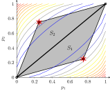
(a) $P_{X}(x_{1})=P_{X}(x_{2})$

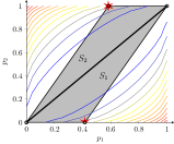
(b) $P_{X}(x_{1})=0.8$.

Figure 2: Geometry of the binary input binary output optimization problem for different prior configuration and $\epsilon=\log 1.5$. Contour lines show mutual information between source alphabet and the variable induced by the mechanism. Stars mark optimal solutions. Note that 2(b) corresponds to a case where $e^{\epsilon}P_{X}(x_{1})\geq 1$, that is, a case with an active box constraint. 2(a) corresponds to a case with no active box constraints. The dividing line indicates the regions $S_{1}$,$S_{2}$.

-E Proof of Theorem 3

Throughout the proof we will refer to output alphabet size as the effective size of the output alphabet, that is, the size of the support set of the output $Y$. As discussed in Section III-C, we will generally consider the mechanism $\bm{P}=P_{Y|X}$ to be a $N\times N$ matrix. We say that a mechanism $\bm{Q}$ has a smaller output alphabet size than $\bm{P}$ if $\bm{Q}$ has more all-zero columns than $\bm{P}$, implying $\textnormal{supp}(Q_{Y|X})<\textnormal{supp}(P_{Y|X})$.

For simplicity, each step in the proof is given as a separate lemma. We start by establishing the overall structure of the extremal mechanisms. Since extremal mechanisms are the extreme points of the polytope $\mathcal{M}_{N}(\epsilon)$, they satisfy $N^{2}$ of the constraints in (16) with equality. Note that all privacy mechanisms (extremal or not) satisfy the $N$ equality constraints of (16b). Therefore, the distinguishing factor for extremal mechanisms is that they also satisfy $N(N-1)$ of the inequality constraints in (16a) or (16c) with equality. This fact is frequently used in the proof.

Throughout this section, we will refer to extremal elements as the elements of a mechanism that meet a PML constraint with equality. We call an element $p_{ij}$ of a mechanism $P_{Y|X}$ extremal if $\frac{p_{ij}}{P_{Y}(y_{j})}=e^{\epsilon}$, where $i,j\in[N]$.

Lemma 3.

If $P_{Y|X}\in\mathcal{M}_{N}(\epsilon)$ is extremal, then each $y_{j}$ fulfills exactly $N-1$ PML constraints with equality and the index $i\in[N]$ of the non-extremal element $p_{ij}$ is different for every $j\in[N]$.

Proof.

Firstly, assume $\epsilon>0$, since otherwise there is nothing to prove and we have the trivial optimal solution of $X\operatorname*{\perp\!\!\!\perp}Y$, that is, $P_{Y|X=x}(y)=\text{const}$. We prove this lemma by contradiction: For each outcome $j\in[N]$, we use $r(j)\in[N]$ to denote the index of a non-extremal element. We prove that all elements in column $j$ of the mechanism are equal except for the $r(j)$-th element. That is,

$$p_{ij}=p_{i^{\prime}j},\quad\forall i,i^{\prime}\in[N]\text{ and }i,i^{\prime}\neq r(j).$$ (40)

We also show that $r(j)\neq r(j^{\prime})\text{ for }j\neq j^{\prime}$.

Note that as a result of Lemma 2, mechanisms in the high-privacy region $\epsilon<\log\frac{1}{1-p_{\min}}$ cannot contain elements equal to zero or one (except if we have an all-zeros column). Therefore, when $|\mathcal{Y}|=|\mathcal{X}|$, a mechanism can only be extremal by fulfilling exactly $N(N-1)$ of the PML constraints (16a) with equality. Now, assume there exists some outcome $y_{j}$ that fulfills $N-k$ of the PML constraints with $k\geq 2$. Then, in order to meet $N(N-1)$ privacy constraints, there must be $(k-1)$ outcomes each satisfying $N$ privacy constraints with equality. Suppose $y_{1}$ is such an outcome. Then, $p_{i1}=p_{i^{\prime}1}$ for all $i,i^{\prime}\in[N]$ and

$$\ell(X\rightarrow y_{1})=\log\biggl{(}\frac{p_{11}}{p_{11}\sum_{x}P_{X}(x)}\biggr{)}=0,$$ (41)

i.e., $y_{1}$ meets no PML constraints which is a contradiction. This shows that each outcome of the privacy mechanism must satisfy exactly $N-1$ PML constraints.

What is left to show that $r(j)\neq r(j^{\prime})\text{ for }j\neq j^{\prime}$ holds. Again, we can construct a simple contradiction: Assume there exists $j\neq j^{\prime}$ such that $r(j)=r(j^{\prime})$. Since each column needs to fulfill $N-1$ PML constraints, there will be one row for which all elements are extremal, resulting in a violation of row-stochasticity. For this specific row, say at index $i\in[N]$, every element will be extremal and we get

$$\sum_{j}p_{ij}=\sum_{j}e^{\epsilon}P_{Y}(y_{j})=e^{\epsilon}>1,$$ (42)

which yields a contradiction, as desired. ∎

In other words, for each $j\in[N]$, $N-1$ of the elements in that column take the same value $p_{ij}=E(j)$, with $E(j)$ denoting the extremal value in column $j$. The remaining element $p_{r(j)j}$ takes the value ensuring that the row-sum constraints are met in each row. There are $N!$ such combinations, that all belong to the same equivalence class according to Remark 1, that is, they are equivalent up to column permutations. To illustrate this, consider $N=3$. Two of the possible solutions are

$$\begin{bmatrix}p_{r(1)1}&E(2)&E(3)\\ E(1)&p_{r(2)2}&E(3)\\ E(1)&E(2)&p_{r(3)3}\end{bmatrix},\quad\begin{bmatrix}E(3)&E(2)&p_{r(1)1}\\ E(3)&p_{r(2)2}&E(1)\\ p_{r(3)3}&E(2)&E(1)\end{bmatrix}.$$ (43)

Lemma 4.

A mechanism with $|\mathcal{Y}|=|\mathcal{X}|-k$, that is, with $k$ all-zero columns, can only be an extreme point of the bounding PML polytope if it is composed of the elements $p_{ij}\in\{E(j),\tilde{E}(j)\},\,\forall j\in[N]$, where $E(j)$ meets the PML constraint with equality for the corresponding column $j$, and $\tilde{E}(j)$ ensures the mechanism’s row-stochasticity. Further, in each column $j$ there are $m_{j}$ elements $\tilde{E}(j)$, with

$$m_{j}\in\{1,\dots,k+1\},\quad\sum_{j\in[N]}m_{j}=N,$$ (44)

and any row contains exactly one of those elements.

Proof.

Without loss of generality, assume a mechanism for which the $k$ last columns are all-zero columns. Consider the first column (which is not all zero). Clearly, from equation (41), the maximum number of extremal elements in any non-zero column is upper bounded by $N-1$. The number of overall inequality constraints all columns except the first one can fulfill with equality is therefore upper bounded by

$$kN+(N-k-1)(N-1)=N^{2}-N-(N-(k+1)).$$ (45)

Recall that in order to be an extreme point, any mechanism needs to fulfill $N^{2}-N$ inequality constraints with equality. This yields the lower bound on the number of extremal elements in the first column to be $N-(k+1)$. This applies identically to all of the first $N-k$ columns. The structure of the extremal mechanisms is therefore fixed up to the degrees of freedom provided by the choice of element combinations while staying in the provided bounds on extremal elements per column, or equivalently on the values $m_{j}$. ∎

For illustration, consider again the case $N=3$: Assuming that the column meeting $N-2$ constraints is column $j=2$, we get

$$\begin{bmatrix}E(1)&\tilde{E}(2)&0\\ E(1)&\tilde{E}(2)&0\\ \tilde{E}(1)&E(2)&0\end{bmatrix},\quad\begin{bmatrix}\tilde{E}(1)&E(2)&0\\ E(1)&\tilde{E}(2)&0\\ E(1)&\tilde{E}(2)&0\end{bmatrix}$$ (46)

as two example configurations.

Lemma 5.

Assume an extremal mechanism $\bm{P}$ structured as in Lemma 3 and a stochastic mapping $\bm{W}$, which merges two of $\bm{P}$’s non-zero columns $\bm{P}_{u}$, $\bm{P}_{v}$ into one. Then the mechanism $\bm{W}\circ\bm{P}$ is also extremal.

Proof.

Assume the two columns merged fulfill $N-k$ and $N-l$ PML constraints with equality, respectively. Let $\sum_{i}p_{ij}P_{X}(x_{i})\coloneqq\Sigma_{j}$ and recall that $(\bm{P}_{j})_{i}=P_{Y|X=x_{i}}(y_{j})\coloneqq p_{ij}$. Then from the PML constraints we have

$$E(j)\coloneqq\max_{i\in[N]}\,p_{ij}=e^{\epsilon}\Sigma_{j},\,j=u,v$$ (47)

and therefore

$$\exp(\ell_{\bm{W}\circ\bm{P}}(X\to y)) =\frac{E(u)+E(v)}{\sum_{i}(\bm{P}_{u}+\bm{P}_{v})_{i}P_{X}(x_{i})}$$ (48)

$$=\frac{E(u)+E(v)}{\Sigma_{u}+\Sigma_{v}}=\frac{e^{\epsilon}\Sigma_{u}+e^{\epsilon}\Sigma_{v}}{\Sigma_{u}+\Sigma_{v}}=e^{\epsilon}.$$

Further, by Lemma 4 the positions $r(j)$, $r(j^{\prime})$ of the non-extremal elements are different for any two columns $j\neq j^{\prime}$. Because of this, there will be a total of $k+l$ of non-extremal elements in the merged column, that is, equation (48) holds for exactly $N-(k+l)$ elements of the new non-zero column. Now, from the assumption that $\bm{P}$ is extremal, we know that it fulfills $N^{2}-N$ inequality constraints with equality. Since the column merge yields an additional all-zero column fulfilling $N$ non-negativity constraints with equality, the mechanism $(\bm{W}\circ\bm{P})$ will meet

$$N^{2}-N- ((N-k)+(N-l))$$ (49)

$$+N+(N-(k+l))=N^{2}-N$$

inequality constraints with equality, that is, the mechanism created from merging any two non-zero columns of $\bm{P}$ is another vertex of $\mathcal{M}_{N}(\epsilon)$. ∎

Lemma 6.

Any extremal mechanism $Q_{Y|X}$ with alphabet size $|\mathcal{Y}|=N-k$ can be obtained from an extremal mechanism $P_{Y|X}$ with alphabet size $|\mathcal{Y}|=N-k+1$ by merging two of its columns into one.

Proof.

Suppose the first column of $Q_{Y|X}$ satisfies $N-m$ PML constraints with equality, where $1<m\leq k+1$. Then there exists $s,t\geq 1$ such that $m=s+t$. Hence, we can construct $P_{Y|X}$ such that it has a column satisfying $N-s$ PML constraints, and an additional column satisfying $N-t$ constraints, while all other columns are identical to the columns in $Q_{Y|X}$. With this, the mechanism $P_{Y|X}$ has an output alphabet size one larger than $Q_{Y|X}$. At the same time, Lemma 5 shows that we can obtain $Q_{Y|X}$ from the mechanism $P_{Y|X}$ constructed in this way by merging the two newly constructed columns into one. From Lemma 5 we also know that, if $P_{Y|X}$ is extremal, $Q_{Y|X}$ is also extremal. ∎

Lemma 7.

Assume that a mechanism $P_{Y|X}$ satisfies $\epsilon$-PML and has no all-zero column, that is, $P_{Y|X=x_{i}}(y_{j})\neq 0,\,\forall i,j\in[N]$. Assume further that $P_{Y|X}$ is extremal in the sense that it follows the structure presented in Lemma 3. Then any mechanism $Q_{Y|X}$ that satisfies $\epsilon$-PML and contains a zero column, that is, $\exists j\in[N]:Q_{Y|X=x_{i}}(y_{j})=0,\,\forall i\in[N]$, will not have higher utility given any sub-convex utility function. I.e.,we have

$$U(Q_{Y|X})\leq U(P_{Y|X}).$$ (50)

Proof.

Lemma 6 shows inductively that any extreme point of the bounding polytope of the optimization problem can be expressed by recursively merging two columns of an extremal mechanism with $|\mathcal{X}|=|\mathcal{Y}|$ into one while keeping all other columns as they are. In other words, for each extremal mechanism $\bm{Q}$ with support size $N-k$ there exists an extremal mechanism $\bm{P}$ with support size $N-k+1$ and a kernel $\bm{W}$ such that $\bm{Q}=\bm{W}\circ\bm{P}$. Therefore, by the data processing inequality for sub-convex functions [34, Proposition 17], extremal mechanisms with $|\mathcal{Y}|<|\mathcal{X}|$ cannot have higher utility than extremal mechanisms with $|\mathcal{Y}|=|\mathcal{X}|$.

∎

As previously pointed out, Lemma 1 implies that the optimal solution to the optimization problem (13) is one of the extremal mechanisms characterized in the above lemmas. Lemma 7 then shows that in the high-privacy regime, all extremal mechanisms with $M<N$ can be disregarded. Notice that, given one of the structured matrices presented in Lemma 3, the values of $E(j)$ and $\tilde{E}(j)$ are unique. Therefore, the solution to the maximization problem is unique up to column-permutations of the structured matrices. Since by the fact that all column permutations of a mechanism preserve its utility, any solution corresponding to one of the structured matrices is an optimal solution. Noticing that the mechanism $P^{*}_{Y|X}$ in Theorem 3 has the required structure, and meets $N(N-1)$ inequality constraints with equality, proofs that all mechanisms in its equivalence class $[P^{*}_{Y|X}]$ are optimal in the high-privacy regime. ∎

-F Proof of Theorem 4

For notational simplicity, denote by $\bm{\pi}$ and $\bm{\rho}$ the probability mass functions $P_{X}$ and $P_{Y}$, respectively.

Using the homogeneity of sub-linear functions, we can upper bound any sub-convex utility as

$$U(\bm{P}) =\sum_{j=1}^{N}\mu(\bm{P}_{j})=\sum_{j=1}^{N}\mu\biggl{(}\rho_{j}\bm{\lambda}_{j}\biggr{)}$$ (51)

$$=\sum_{j=1}^{N}\rho_{j}\mu\biggl{(}\bm{\lambda}_{j}\biggr{)}=\mathbb{E}_{Y}\biggl{\{}\mu\biggl{(}\bm{\lambda}_{j}\biggr{)}\biggr{\}}$$ (52)

$$\leq\max_{j\in[N]}\,\mu\biggl{(}\bm{\lambda}_{j}\biggr{)},$$ (53)

where $(\lambda_{ij})=(\bm{\lambda}_{j})_{i}\eqqcolon\bm{\Lambda}$ denotes the lift-matrix, which we define using the information density $i(x;y)$ as

$$\lambda_{ij}\coloneqq\exp(i(x_{i};y_{j}))\quad\forall i,j\in[N].$$ (54)

Further, from the PML constraints we have

$$i(x_{i};y_{j})\leq\epsilon\quad\forall i,j\in[N]$$ (55)

and since $\mu$ is convex and symmetric, it is Schur-convex [35]. Fix some arbitrary $j\in[N]$. Under the given constraints ($\epsilon$-PML, row-stochasticity), $\mu$ will be maximized by the vector $\bm{\lambda}^{*}_{j}$ that majorizes all other vectors $\bm{\lambda}_{j}$ satisfying these constraints for some $j\in[N]$. That is, we have $\bm{\lambda}_{j}^{*}\succeq\bm{\lambda}_{j}$. Since $\epsilon$ is in the $k^{\text{th}}$ privacy region, we know that it can contain no more than $k-1$ zero elements. Further, by (55), the maximum value each of the elements in $\bm{\Lambda}$ can take is $e^{\epsilon}$. Let $[\bm{\lambda}_{j}]$ denote the set of all element permutations of $\bm{\lambda}_{j}$ for some fixed $j$. Then we have

$$[\bm{\lambda}^{*}_{j}]=[(\underbrace{e^{\epsilon},\dots,e^{\epsilon}}_{{N-k}\text{ times }},r,\underbrace{0,\dots,0}_{k-1\text{ times }})^{T}],$$ (56)

where we get the value of $r$ from the constraint

$$\sum_{x\in\mathcal{X}}P_{X|Y=y}(x)=\sum_{i=1}^{N}\lambda_{ij}\pi_{i}=\sum_{i=1}^{N}\frac{\lambda_{ij}}{N}=1$$ (57)

as $r=N-(N-k)e^{\epsilon}$. Note that the value of $r$ is independent of the value of $j$. Hence, we obtain $U(\bm{P})\leq\mu(\bm{\lambda}^{*}_{j})$ as an upper bound on the optimal utility. It can be verified that the mechanism given in (20) attains this bound; thus, it is optimal. ∎

-G Proof of Theorem 5

Let $\bm{\rho}$, $\bm{\pi}$ and $\bm{\Lambda}$ be defined as in Appendix -F. First, consider the following reformulation of problem (13):

$$\max_{\bm{\Lambda},\bm{\rho}}\,U(\bm{\Lambda},\bm{\rho}) =\sum_{j=1}^{N}\mu\biggl{(}\rho_{j}\bm{\lambda}_{j}\biggr{)}=\sum_{j=1}^{N}\rho_{j}\mu\biggl{(}\bm{\lambda}_{j}\biggr{)}$$ (58a)

s.t. $$\sum_{j=1}^{N}\rho_{j}\lambda_{ij}=1\quad\forall i\in[N],$$ (58b)

$$\sum_{i=1}^{N}\pi_{i}\lambda_{ij}=1\quad\forall j\in[N],$$ (58c)

$$0\leq\lambda_{ij}\leq e^{\epsilon}\,\forall i,j\in[N].$$ (58d)

Note that (58b) and (58c) together imply $\sum_{y}P_{Y}(y)=1$. Next, we show that the columns of the optimal lift-matrix $\bm{\Lambda}^{*}$ belong to the set $\bm{\Lambda}^{*}(k,P_{X})$. To see why, let $\bm{\rho}^{*}$ denote the optimal distribution in problem (58a). Given this distribution, we find the values of $\bm{\lambda}^{*}_{j}$ by solving the problem

$$\max_{\bm{\Lambda}}\,U(\bm{\Lambda},\bm{\rho}^{*}) =\sum_{j=1}^{N}\rho^{*}_{j}\mu\biggl{(}\bm{\lambda}_{j}\biggr{)}$$ (59a)

s.t. $$\sum_{j=1}^{N}\rho^{*}_{j}\lambda_{ij}=1\quad\forall i\in[N],$$ (59b)

$$\sum_{i=1}^{N}\pi_{i}\lambda_{ij}=1\quad\forall j\in[N],$$ (59c)

$$0\leq\lambda_{ij}\leq e^{\epsilon}\,\forall i,j\in[N].$$ (59d)

Since we are maximizing a convex function over a polytope, the optimal utility value in this setup is attained by a vertex of the polytope. To characterize these vertices, denote by $\tilde{\bm{\pi}}(\bm{\lambda}_{j})$ the subset of prior probabilities of all symbols to which $\bm{\lambda}_{j}$ assigns a non-zero lift-value, that is,

$$\tilde{\bm{\pi}}(\bm{\lambda}_{j})\coloneqq\{\pi_{i}\in\bm{\pi}:\lambda_{ij}>0\}.$$ (60)

Then, substituting into (59c) and upper bounding with (59d) yields the following condition on the probability mass of this set

$$\sum_{i=1}^{N}\pi_{i}\lambda_{ij}=\sum_{i=1}^{|\tilde{\bm{\pi}}(\bm{\lambda}_{j})|}\tilde{\pi}_{i}(\bm{\lambda}_{j})\lambda_{ij}\leq\sum_{i=1}^{|\tilde{\bm{\pi}}(\bm{\lambda}_{j})|}\tilde{\pi}_{i}(\bm{\lambda}_{j})e^{\epsilon}=1,$$ (61)

thus lower bounding the probability of any such subset implied by a vector $\bm{\lambda}_{j}$ satisfying $\epsilon$-PML as

$$\sum_{\pi\in\tilde{\bm{\pi}(\bm{\lambda}_{j})}}\pi\geq e^{-\epsilon}.$$ (62)

Define the subset of lift-vectors with $l$ non-zero elements and fulfilling condition (62) as

$$\tilde{\bm{\Lambda}}(l)\coloneqq\{\bm{\lambda}_{j}:\sum_{\pi\in\tilde{\bm{\pi}}(\bm{\lambda}_{j})}\pi\geq e^{-\epsilon}\text{ and }|\tilde{\bm{\pi}}(\bm{\lambda}_{j})|=l\}.$$ (63)

Note that, for determining the extremality conditions on these vectors, we can apply the same chain of arguments as applied in the proof of Theorem 3. That is, there exists an optimal $N\times N$ mechanism $P^{*}_{Y|X}$ for which all $N$ columns meet exactly $N-1$ inequality constraints with equality. Denote the set of all such vectors in the set $\tilde{\bm{\Lambda}}(l)$ as $\tilde{\bm{\Lambda}}^{*}(l)$. Then we get the set of all extreme points of the bounding polytope that fulfill $N-1$ inequality constraints with equality in the $k^{\text{th}}$ privacy region as $\tilde{\bm{\Lambda}}^{*}\coloneqq\bigcup_{l=0}^{k-1}\tilde{\bm{\Lambda}}^{*}(l)=\bm{\Lambda}^{*}(k,P_{X})$. Due to the convexity of the objective function, and given $\bm{\rho}^{*}$ as the optimal distribution on $Y$, it is possible to construct a maximizing solution $\bm{\Lambda}^{*}$ using only lift-vectors out of the set $\tilde{\bm{\Lambda}}^{*}$.

Now, all that is left to show is that the optimal distribution on $Y$ can be found by the original optimization problem. Assume the optimal lift-matrix $\bm{\Lambda}^{*}$ to be known and let the optimal utility values of column $j$ implied by this solution be denoted by $\mu^{*}_{j}\,\forall j\in[N]$. Then the objective function becomes

$$\max_{\bm{\rho}}\,U(\bm{\Lambda}^{*},\bm{\rho})=\sum_{j=1}^{N}\rho_{j}\mu^{*}_{j},$$ (64)

which is a linear function of $\bm{\rho}$. Together with the above derivations, this proves the result. ∎

References

- Nissim and Wood [2018] K. Nissim and A. Wood, “Is privacy privacy?” Philos. Trans. R. Soc., A, vol. 376, no. 2128, p. 20170358, 2018.
- Nissim and Wood [2021] ——, “Foundations for robust data protection: Co-designing law and computer science,” in IEEE TPS-ISA 2021, 2021, pp. 235–242.
- Erlingsson et al. [2014] Ú. Erlingsson et al., “Rappor: Randomized aggregatable privacy-preserving ordinal response,” in ACM SIGSAC CCS 2014, 2014.
- Apple Differential Privacy Team [2017] Apple Differential Privacy Team, “Learning with privacy at scale,” 2017. [Online]. Available: https://api.semanticscholar.org/CorpusID:43986173
- Dwork et al. [2014] C. Dwork et al., “The algorithmic foundations of differential privacy,” Found. Trends Theor. Comput. Sci., vol. 9, no. 3–4, pp. 211–407, 2014.
- Evfimievski et al. [2003] A. Evfimievski et al., “Limiting privacy breaches in privacy preserving data mining,” in Proc. 22nd ACM SIGMOD-SIGACT-SIGART PODS, 2003, pp. 211–222.
- Kasiviswanathan et al. [2008] S. P. Kasiviswanathan et al., “What can we learn privately?” in 49th IEEE FOCS, 2008, pp. 531–540.
- Tschantz et al. [2020] M. C. Tschantz, S. Sen, and A. Datta, “Sok: Differential privacy as a causal property,” in IEEE S&P, 2020, pp. 354–371.
- Ghosh and Kleinberg [2016] A. Ghosh and R. Kleinberg, “Inferential privacy guarantees for differentially private mechanisms,” arXiv preprint arXiv:1603.01508, 2016.
- Kifer and Machanavajjhala [2011] D. Kifer and A. Machanavajjhala, “No free lunch in data privacy,” in Proc. ACM SIGMOD Int. Conf. Manag. Data, 2011, pp. 193–204.
- Yang et al. [2015] B. Yang et al., “Bayesian differential privacy on correlated data,” in Proc. ACM SIGMOD Int. Conf. Manag. Data, 2015, pp. 747–762.
- Zhu et al. [2014] T. Zhu et al., “Correlated differential privacy: Hiding information in non-iid data set,” IEEE TIFS, vol. 10, no. 2, pp. 229–242, 2014.
- Dwork et al. [2019] C. Dwork, N. Kohli, and D. Mulligan, “Differential privacy in practice: Expose your epsilons!” J. Priv. Confidentiality, vol. 9, no. 2, 2019.
- Asoodeh et al. [2015] S. Asoodeh, F. Alajaji, and T. Linder, “On maximal correlation, mutual information and data privacy,” in IEEE CWIT, 2015, pp. 27–31.
- Wang et al. [2016] W. Wang, L. Ying, and J. Zhang, “On the relation between identifiability, differential privacy, and mutual-information privacy,” IEEE Trans. Inf. Theory, vol. 62, no. 9, pp. 5018–5029, 2016.
- Issa et al. [2019] I. Issa, A. B. Wagner, and S. Kamath, “An operational approach to information leakage,” IEEE Transactions on Information Theory, 2019.
- Liao et al. [2019] J. Liao et al., “Tunable measures for information leakage and applications to privacy-utility tradeoffs,” IEEE Trans. Inf. Theory, 2019.
- Sibson [1969] R. Sibson, “Information radius,” Zeitschrift für Wahrscheinlichkeitstheorie und verwandte Gebiete, vol. 14, no. 2, pp. 149–160, 1969.
- Zarrabian et al. [2023] M. A. Zarrabian, N. Ding, and P. Sadeghi, “On the lift, related privacy measures, and applications to privacy–utility trade-offs,” Entropy, vol. 25, no. 4, p. 679, 2023.
- Jiang et al. [2020] B. Jiang, M. Li, and R. Tandon, “Local information privacy and its application to privacy-preserving data aggregation,” IEEE Trans. Dependable Secure Comput., vol. 19, no. 3, pp. 1918–1935, 2020.
- Asoodeh et al. [2018] S. Asoodeh, M. Diaz, F. Alajaji, and T. Linder, “Estimation efficiency under privacy constraints,” IEEE Trans. Inf. Theory, 2018.
- Rassouli and Gündüz [2019] B. Rassouli and D. Gündüz, “Optimal utility-privacy trade-off with total variation distance as a privacy measure,” IEEE TIFS, 2019.
- Diaz et al. [2020] M. Diaz et al., “On the robustness of information-theoretic privacy measures and mechanisms,” IEEE Trans. Inf. Theory, 2020.
- Bloch et al. [2021] M. Bloch et al., “An overview of information-theoretic security and privacy: Metrics, limits and applications,” IEEE JSAIT, vol. 2, 2021.
- Wagner and Eckhoff [2018] I. Wagner and D. Eckhoff, “Technical privacy metrics: A systematic survey,” ACM Comput. Surv., vol. 51, no. 3, 2018.
- Alvim et al. [2020] M. S. Alvim et al., The Science of Quantitative Information Flow. Springer, 2020.
- Alvim et al. [2012] ——, “Measuring information leakage using generalized gain functions,” in IEEE 25th Comp. Security Found. Symp., 2012.
- Saeidian et al. [2023a] S. Saeidian, G. Cervia, T. J. Oechtering, and M. Skoglund, “Pointwise maximal leakage,” IEEE Trans. Inf. Theory, 2023.
- Saeidian et al. [2023b] ——, “Pointwise maximal leakage on general alphabets,” arXiv preprint arXiv:2304.07722, 2023.
- Saeidian et al. [2023c] ——, “Inferential privacy: From impossibility to database privacy,” arXiv preprint arXiv:2303.07782, 2023.
- Rényi [1961] A. Rényi, “On measures of entropy and information,” in Proceedings of the Fourth Berkeley Symposium on Mathematical Statistics and Probability, Volume 1: Contributions to the Theory of Statistics, vol. 4. University of California Press, 1961, pp. 547–562.
- Dwork et al. [2006] C. Dwork, F. McSherry, K. Nissim, and A. Smith, “Calibrating noise to sensitivity in private data analysis,” in Theory of Cryptography: Third Theory of Cryptography Conference, TCC 2006, New York, NY, USA, March 4-7, 2006. Proceedings 3. Springer, 2006, pp. 265–284.
- Warner [1965] S. L. Warner, “Randomized response: A survey technique for eliminating evasive answer bias,” Journal of the American Statistical Association, vol. 60, no. 309, pp. 63–69, 1965, pMID: 12261830.
- Kairouz et al. [2016] P. Kairouz, S. Oh, and P. Viswanath, “Extremal mechanisms for local differential privacy,” The Journal of Machine Learning Research, vol. 17, no. 1, pp. 492–542, 2016.
- Marshall et al. [2011] A. W. Marshall, I. Olkin, and B. C. Arnold, Inequalities: Theory of Majorization and its Applications, 2nd ed. Springer, 2011, vol. 143.
- Kalantari et al. [2018] K. Kalantari, L. Sankar, and A. D. Sarwate, “Robust privacy-utility tradeoffs under differential privacy and hamming distortion,” IEEE TIFS, vol. 13, no. 11, 2018.
- Duchi et al. [2013] J. C. Duchi, M. I. Jordan, and M. J. Wainwright, “Local privacy and statistical minimax rates,” in IEEE FOCS, 2013.
- Acharya et al. [2020] J. Acharya et al., “Context aware local differential privacy,” in Int. Conf. on Machine Learning. PMLR, 2020, pp. 52–62.
- Hsu et al. [2019] H. Hsu, S. Asoodeh, and F. P. Calmon, “Information-theoretic privacy watchdogs,” in IEEE Int. Symp. Inf. Theory, 2019, pp. 552–556.
- Zarrabian et al. [2022] M. A. Zarrabian, N. Ding, and P. Sadeghi, “Asymmetric local information privacy and the watchdog mechanism,” in 2022 IEEE Information Theory Workshop (ITW), 2022, pp. 7–12.
- Jiang et al. [2021] B. Jiang, M. Seif, R. Tandon, and M. Li, “Context-aware local information privacy,” IEEE Transactions on Information Forensics and Security, vol. 16, pp. 3694–3708, 2021.
- Lopuhaä-Zwakenberg [2020] M. Lopuhaä-Zwakenberg, “The privacy funnel from the viewpoint of local differential privacy,” arXiv preprint arXiv:2002.01501, 2020.
- Saeidian et al. [2021] S. Saeidian, G. Cervia, T. J. Oechtering, and M. Skoglund, “Optimal maximal leakage-distortion tradeoff,” in 2021 IEEE Information Theory Workshop (ITW). IEEE, 2021, pp. 1–6.
- Wu et al. [2020] B. Wu, A. B. Wagner, and G. E. Suh, “Optimal mechanisms under maximal leakage,” in 2020 IEEE Conference on Communications and Network Security (CNS), 2020, pp. 1–6.
- Liao et al. [2017] J. Liao, L. Sankar, F. P. Calmon, and V. Y. F. Tan, “Hypothesis testing under maximal leakage privacy constraints,” in 2017 IEEE International Symposium on Information Theory (ISIT), 2017, pp. 779–783.
- El Gamal and Kim [2011] A. El Gamal and Y.-H. Kim, Network information theory. Cambridge university press, 2011.
- Griva et al. [2009] I. Griva, S. G. Nash, and A. Sofer, Linear and nonlinear optimization, 2nd ed. SIAM, 2009.
- Payne and Ives [1979] W. H. Payne and F. M. Ives, “Combination generators,” ACM TOMS, vol. 5, no. 2, pp. 163–172, 1979.
- Boyd and Vandenberghe [2014] S. P. Boyd and L. Vandenberghe, Convex Optimization. Cambridge University Press, 2014.