Score Regularized Policy Optimization
through Diffusion Behavior

Abstract

Recent developments in offline reinforcement learning have uncovered the immense potential of diffusion modeling, which excels at representing heterogeneous behavior policies. However, sampling from diffusion policies is considerably slow because it necessitates tens to hundreds of iterative inference steps for one action. To address this issue, we propose to extract an efficient deterministic inference policy from critic models and pretrained diffusion behavior models, leveraging the latter to directly regularize the policy gradient with the behavior distribution’s score function during optimization. Our method enjoys powerful generative capabilities of diffusion modeling while completely circumventing the computationally intensive and time-consuming diffusion sampling scheme, both during training and evaluation. Extensive results on D4RL tasks show that our method boosts action sampling speed by more than 25 times compared with various leading diffusion-based methods in locomotion tasks, while still maintaining state-of-the-art performance. Code: https://github.com/thu-ml/SRPO.

Figure 1: Performance and computational efficiency of different algorithms in D4RL Locomotion tasks. Computation time is assessed using a consistent hardware setup and PyTorch backend.

1 Introduction

Offline reinforcement learning (RL) aims to tackle decision-making problems by solely utilizing a pre-collected behavior dataset. This offers a practical solution for tasks where data collection can be associated with substantial risks or exorbitant costs. A central challenge for offline RL is the realization of behavior regularization, which entails ensuring the learned policy stays in support of the behavior distribution. Weighted regression (Peng et al., 2019; Kostrikov et al., 2022) provides a promising approach that directly utilizes behavioral actions as sources of supervision for policy training. Another prevalent approach is behavior-regularized policy optimization (Kumar et al., 2019; Wu et al., 2019), which builds a generative behavior model, followed by constraining the divergence between the learned and the behavior model during policy optimization.

An expressive generative model holds a pivotal role in the aforementioned regularization methods. In weighted regression, a unimodal actor is prone to suffer from the “mode covering” issue, a phenomenon where policies end up selecting out-of-support actions in the middle region between two behavioral modes (Wang et al., 2023a; Hansen-Estruch et al., 2023). Expressive policy classes, with diffusion models (Ho et al., 2020) as prime choices, help to resolve this issue. In behavior-regularized policy optimization, diffusion modeling can also be significantly advantageous for an accurate estimate of policy divergence, due to its strong ability to represent heterogeneous behavior datasets, outperforming conventional methods like Gaussians or variational auto-encoders (VAEs) (Goo & Niekum, 2022; Chen et al., 2023).

However, a major drawback of utilizing diffusion models in offline RL is the considerably slow sampling speed – diffusion policies usually require 5-100 iterative inference steps to create an action sample. Moreover, diffusion policies tend to be excessively stochastic, forcing the generation of dozens of action candidates in parallel to pinpoint the final optimal one (Wang et al., 2023a). As existing methods necessitate sampling from or backpropagating through diffusion policies during training and evaluation, it has significantly slowed down experimentation and limited the application in fields that are computationally sensitive or require high control frequency, such as robotics. Therefore, it is critical to systematically investigate the question: is it feasible to fully exploit the generative capabilities of diffusion models without directly sampling actions from them?

In this paper, we propose Score Regularized Policy Optimization (SRPO) with a positive answer to the above question. The basic idea is to extract a simple deterministic inference policy from critic and diffusion behavior models to avoid the iterative diffusion sampling process during evaluation. To achieve this, we show that the gradient of the divergence term in regularized policy optimization is essentially related to the score function of behavior distribution (Section 3.1). The latter can be effectively approximated by any pretrained score-based model including diffusion models (Song et al., 2021). This allows us to directly regularize the policy gradient instead of the policy loss, removing the need to generate fake behavioral actions for policy-divergence estimation (Section 3.2).

We develop a practical algorithm to solve continuous control tasks (Section 4) by combining SRPO with implicit Q-learning (Kostrikov et al., 2022) and continuous-time diffusion behavior modeling (Lu et al., 2023). For policy extraction, we incorporate similar techniques that have facilitated recent advances in text-to-3D research such as DreamFusion (Poole et al., 2023). These include leveraging an ensemble of score approximations under different diffusion times to exploit the pretrained behavior model and a baseline term to reduce variance for gradient estimation. We empirically show that these techniques successfully help improve performance and stabilize training for policy extraction.

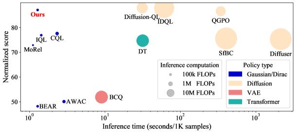
We evaluate our method in D4RL tasks (Fu et al., 2020). Results demonstrate that our method enjoys a more than 25$\times$ boost in action sampling speed and less than $1\%$ of computational cost for evaluation compared with several leading diffusion-based methods while maintaining similar overall performance in locomotion tasks (Figure 1). We also conduct 2D experiments to better illustrate that SRPO successfully constrains the learned policy close to various complex behavior distributions.

2 Background

2.1 Offline Reinforcement Learning

Consider a typical Markov Decision Process (MDP) described by the tuple $\langle\mathcal{S},\mathcal{A},P,r,\gamma\rangle$, where $\mathcal{S}$ is the state space, $\mathcal{A}$ the action space, $P({\bm{s}}^{\prime}|{\bm{s}},{\bm{a}})$ the transition function, $r({\bm{s}},{\bm{a}})$ the reward function and $\gamma$ the discount factor. The goal of reinforcement learning (RL) is to train a parameterized policy $\pi_{\theta}({\bm{a}}|{\bm{s}})$ which maximizes the expected episode return. Offline RL relies solely on a static dataset $\mathcal{D}^{\mu}$ containing interacting history $\{{\bm{s}},{\bm{a}},r,{\bm{s}}^{\prime}\}$ between a behavior policy $\mu({\bm{a}}|{\bm{s}})$ and the environment to train the parameterized policy.

Suppose we can evaluate the quality of a given action by estimating its expected return-to-go using a Q-network $Q_{\phi}({\bm{s}},{\bm{a}})\approx Q^{\pi}({\bm{s}},{\bm{a}}):=\mathbb{E}_{{\bm{s}}_{1}={\bm{s}},{\bm{a}}_{1}={\bm{a}};\pi}[\sum_{n=1}^{\infty}\gamma^{n}r({\bm{s}}_{n},{\bm{a}}_{n})]$, we can formulate the training objective of offline RL as $\max_{\pi}\mathbb{E}_{{\bm{s}}\sim\mathcal{D}^{\mu},{\bm{a}}\sim\pi(\cdot|{\bm{s}})}Q_{\phi}({\bm{s}},{\bm{a}})-\frac{1}{\beta}D_{\mathrm{KL}}\left[\pi(\cdot|{\bm{s}})||\mu(\cdot|{\bm{s}})\right]$ (Wu et al., 2019). Note that a KL regularization term is added mainly to ensure the learned policy stays in support of explored actions. $\beta$ is some temperature coefficient. Previous work (Peters et al., 2010; Peng et al., 2019) has shown that the optimal policy for such an optimization problem is

$$\pi^{*}({\bm{a}}|{\bm{s}}) =\frac{1}{Z({\bm{s}})}\ \mu({\bm{a}}|{\bm{s}})\ \mathrm{exp}\left(\beta Q_{\phi}({\bm{s}},{\bm{a}})\right),$$ (1)

where $Z({\bm{s}})$ is the partition function. The core problem for offline RL now becomes how to efficiently model and sample from the optimal policy distribution $\pi^{*}(\cdot|{\bm{s}})$.

2.2 Optimal Policy Extraction

(a) Behavior dataset

null

(b) Forward KL &

Unimodal policy

(c) Forward KL &

Expressive policy

(d) Reverse KL &

Unimodal policy

Figure 2: Comparison of different policy extraction methods under bandit settings. Forward KL policy extraction is prone to generate out-of-support actions if the policy is not sufficiently expressive (e.g., Gaussians). This can be mitigated either by employing a more expressive policy class or by switching to a reverse KL objective (our method), which demonstrates a mode-seeking nature.

Existing methods to explicitly model $\pi^{*}$ with a parameterized policy $\pi_{\theta}$ can be roughly divided into two main categories—weighted regression and behavior-regularized policy optimization:

$$\min_{\theta}\mathbb{E}_{{\bm{s}}\sim\mathcal{D}^{\mu}}\underbrace{D_{\mathrm{KL}}\left[\pi^{*}(\cdot|{\bm{s}})\middle|\middle|\pi_{\theta}(\cdot|{\bm{s}})\right]}_{\big{\updownarrow}\hskip 36.98866pt\hbox to0.0pt{\text{{Forward} KL}\hss}} \Leftrightarrow\underbrace{\max_{\theta}\mathbb{E}_{({\bm{s}},{\bm{a}})\sim\mathcal{D}^{\mu}}\left[\frac{1}{Z({\bm{s}})}\mathrm{log}\ \pi_{\theta}({\bm{a}}|{\bm{s}})\ e^{\beta Q_{\phi}({\bm{s}},{\bm{a}})}\right]}_{\text{{Weighted Regression}}},$$ (2)

$$\min_{\theta}\mathbb{E}_{{\bm{s}}\sim\mathcal{D}^{\mu}}\underbrace{D_{\mathrm{KL}}\left[\pi_{\theta}(\cdot|{\bm{s}})\middle|\middle|\pi^{*}(\cdot|{\bm{s}})\right]}_{\text{{Reverse} KL}} \Leftrightarrow\underbrace{\max_{\theta}\mathbb{E}_{{\bm{s}}\sim\mathcal{D}^{\mu},{\bm{a}}\sim\pi_{\theta}}Q_{\phi}({\bm{s}},{\bm{a}})-\frac{1}{\beta}D_{\mathrm{KL}}\left[\pi_{\theta}(\cdot|{\bm{s}})||\mu(\cdot|{\bm{s}})\right]}_{\text{{Behavior-Regularized Policy Optimization}}}.$$ (3)

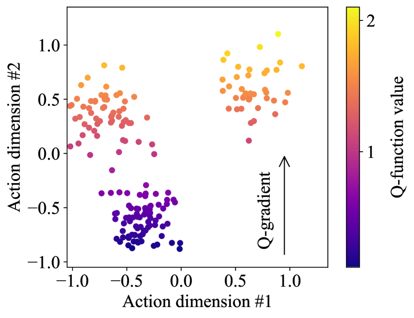
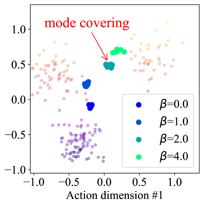
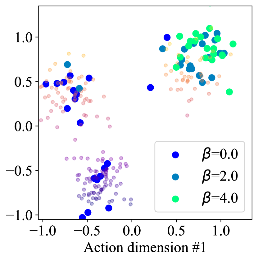
Weighted regression directly utilizes behavioral actions as sources of supervision for policy training. This circumvents the necessity to explicitly model the intricate behavior policy but leads to another mode-covering issue due to the objective’s forward-KL nature (Eq. (2)). The direct consequence is that weighted regression algorithms display sensitivity to the proportion of suboptimal data in the dataset (Yue et al., 2022), especially when the policy model lacks distributional expressivity (Chen et al., 2023), as is depicted in Figure 2. Recent work (Wang et al., 2023a; Lu et al., 2023) attempts to alleviate this by employing more expressive policy classes, such as diffusion models (Ho et al., 2020). However, these methods usually compromise on computational efficiency (Kang et al., 2023).

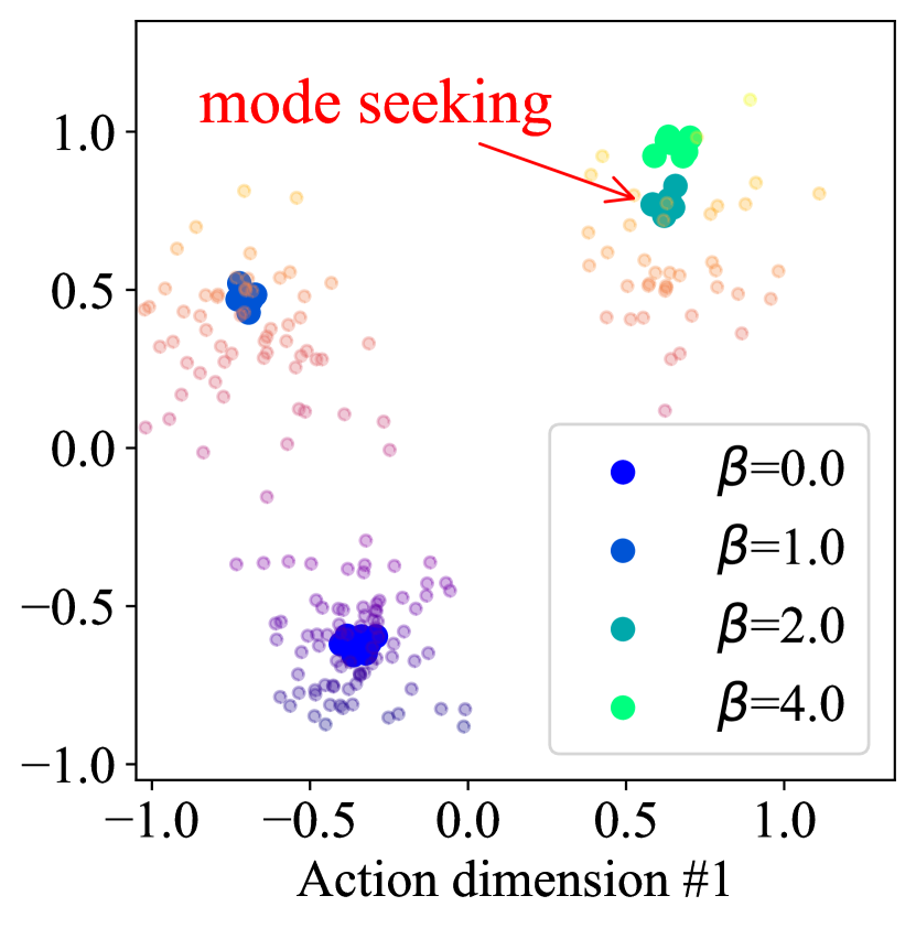
In comparison, behavior-regularized policy optimization (Wu et al., 2019) emerges as a more suitable approach for training simpler policy models such as Gaussian models. This fundamentally stems from its basis on a reverse-KL objective (Eq. (3)), which inherently encourages a mode-seeking behavior. However, approximating the second KL term in Eq. (3) is difficult because only a single action sample ${\bm{a}}$ exists in the behavior dataset $\mathcal{D}^{\mu}$ for any state ${\bm{s}}$ because ${\bm{s}}$ is usually continuous. Regarding this, in practical implementation previous studies (Kumar et al., 2019; Wu et al., 2019; Xu et al., 2021) usually first construct generative behavior models to learn $\mu({\bm{a}}|{\bm{s}})$. Then the learned behavior model is used to generate multiple fake behavioral actions for a given state. Finally, they can approximate the policy-behavior divergence under some metrics such as sampled-based maximum mean discrepancy (MMD, Gretton et al. (2007)) with generated action samples.

2.3 Diffusion Models for Score Function Estimation

Diffusion models (Sohl-Dickstein et al., 2015; Ho et al., 2020; Song et al., 2021) are powerful generative models. They operate by defining a forward diffusion process to perturb the data distribution into a noise distribution for training the diffusion model. Subsequently, this model is employed to reverse the diffusion process, thereby generating data samples from pure noise.

In particular, the forward process is conducted by gradually adding Gaussian noise to samples ${\bm{x}}_{0}$ from an unknown data distribution $q_{0}({\bm{x}}_{0}):=q({\bm{x}})$ at time $0$, forming a series of diffused distributions $q_{t}({\bm{x}}_{t})$ at time $t$. The transition distribution $q_{t0}({\bm{x}}_{t}|{\bm{x}}_{0})$ is:

$$q_{t0}({\bm{x}}_{t}|{\bm{x}}_{0})={\mathcal{N}}({\bm{x}}_{t}|\alpha_{t}{\bm{x}}_{0},\sigma_{t}^{2}{\bm{I}}),\quad\quad\text{which implies}\quad\quad{\bm{x}}_{t}=\alpha_{t}{\bm{x}}_{0}+\sigma_{t}\bm{\epsilon}.$$ (4)

Here, $\alpha_{t},\sigma_{t}>0$ are manually defined, and $\bm{\epsilon}$ is random Gaussian noise.

For the reverse process, Ho et al. (2020) train a diffusion model $\bm{\epsilon}_{\theta}({\bm{x}}_{t}|t)$ to predict the noise added to the diffused sample ${\bm{x}}_{t}$ in order to iteratively reconstruct ${\bm{x}}_{0}$. The optimization problem is

$$\min_{\theta}\mathbb{E}_{t,{\bm{x}}_{0},\bm{\epsilon}}\left[\|\bm{\epsilon}_{\theta}({\bm{x}}_{t}|t)-\bm{\epsilon}\|_{2}^{2}\right].$$ (5)

More formally, Song et al. (2021) show that diffusion models are in essence estimating the score function $\nabla_{{\bm{x}}_{t}}\log q_{t}({\bm{x}}_{t})$ of the diffused data distribution $q_{t}$, such that:

$$\nabla_{{\bm{x}}_{t}}\log q_{t}({\bm{x}}_{t})=-\bm{\epsilon}^{*}({\bm{x}}_{t}|t)/\sigma_{t}\approx-\bm{\epsilon}_{\theta}({\bm{x}}_{t}|t)/\sigma_{t},$$ (6)

and the reverse diffusion process can alternatively be interpreted as discretizing an ODE:

$$\frac{\mathrm{d}{\bm{x}}_{t}}{\mathrm{d}t}=f(t){\bm{x}}_{t}-\frac{1}{2}g^{2}(t)\nabla_{{\bm{x}}_{t}}\log q_{t}({\bm{x}}_{t}),$$ (7)

where $f(t)=\frac{\mathrm{d}\log\alpha_{t}}{\mathrm{d}t},g^{2}(t)=\frac{\mathrm{d}\sigma_{t}^{2}}{\mathrm{d}t}-2\frac{\mathrm{d}\log\alpha_{t}}{\mathrm{d}t}\sigma_{t}^{2}$, leaving $\nabla_{{\bm{x}}_{t}}\log q_{t}({\bm{x}}_{t})$ as the only unknown term. In offline RL, diffusion models have been discovered as an effective tool for modeling heterogeneous behavior policies. Usually states ${\bm{s}}$ are considered as conditions while actions ${\bm{a}}$ are considered as data points ${\bm{x}}$, such that a conditional diffusion model $\bm{\epsilon}({\bm{a}}_{t}|{\bm{s}},t)$ can be constructed to represent $\mu({\bm{a}}|{\bm{s}})$.

3 Score Regularized Policy Optimization

In this section, we describe the main motivation and the high-level idea for our proposed algorithm.

3.1 Challenges for Behavior Regularization

As illustrated in Figure 2 and elaborated in Section 2.2, aside from utilizing a more expressive class of inference policy, another viable strategy to circumvent the mode-covering issue is to employ a reverse-KL policy extraction scheme:

$$\max{\mathcal{L}}_{\pi}(\theta) =\mathbb{E}_{{\bm{s}}\sim\mathcal{D}^{\mu},{\bm{a}}\sim\pi_{\theta}}Q_{\phi}({\bm{s}},{\bm{a}})-\frac{1}{\beta}D_{\mathrm{KL}}\left[\pi_{\theta}(\cdot|{\bm{s}})||\mu(\cdot|{\bm{s}})\right].$$ (8)

A central challenge in optimizing ${\mathcal{L}}_{\pi}(\theta)$ is how to effectively measure the divergence-term in Eq. (8), which is a focal point of extensive previous research (Kumar et al., 2019; Wu et al., 2019; Xu et al., 2021; Wu et al., 2022). A prevalent approach is to use sample-based methods: first constructing a behavioral model $\mu$, followed by sampling fake actions from $\mu$ to approximate the policy divergence. However, this approach necessitates sampling from the behavior model during training, imposing a substantial computational burden. This drawback is exacerbated when employing expressive yet sampling-expensive behavior models such as diffusion models. Unfortunately, adopting an expressive behavior model to represent the potentially diverse behaviors and sampling a significant number of actions for Monte Carlo estimation are both indispensable components of existing methods.

By decomposing the KL term in Eq. (8), we can get

$${\mathcal{L}}_{\pi}(\theta)=\underbrace{\mathbb{E}_{{\bm{s}}\sim\mathcal{D}^{\mu},{\bm{a}}\sim\pi_{\theta}}Q_{\phi}({\bm{s}},{\bm{a}})}_{\text{Policy optimization}}+\ \frac{1}{\beta}\underbrace{\mathbb{E}_{{\bm{s}}\sim\mathcal{D}^{\mu},{\bm{a}}\sim\pi_{\theta}}{\color[rgb]{0,0,1}\log\mu({\bm{a}}|{\bm{s}})}}_{\text{Behavior regularization}}+\frac{1}{\beta}\underbrace{\mathbb{E}_{{\bm{s}}\sim\mathcal{D}^{\mu}}\mathcal{H}(\pi_{\theta}(\cdot|{\bm{s}}))}_{\text{Entropy (often constant)}}.$$ (9)

Eq. (9) unveils that the intrinsic challenge in implementing this training loss rests in the density estimation problem of the behavior policy $\mu({\bm{a}}|{\bm{s}})$, which itself stands as a fundamental topic of generative modeling (Bishop & Nasrabadi, 2006).

3.2 Regularizing Policy Gradient through Pretrained Diffusion Behavior

Our key insight is that a pretrained diffusion behavior model can be leveraged to realize the behavior regularization in Eq. (9). Specifically, we can calculate the gradient of Eq. (9) under the condition that $\pi_{\theta}$ is deterministic. Applying the chain rule and the reparameterization trick, we have:

$$\nabla_{\theta}{\mathcal{L}}_{\pi}(\theta)=\mathbb{E}_{{\bm{s}}\sim\mathcal{D}^{\mu}}\left[\nabla_{{\bm{a}}}Q_{\phi}({\bm{s}},{\bm{a}})|_{{\bm{a}}=\pi_{\theta}({\bm{s}})}+\frac{1}{\beta}{\color[rgb]{0,0,1}\underbrace{\nabla_{{\bm{a}}}\log\mu({\bm{a}}|{\bm{s}})|_{{\bm{a}}=\pi_{\theta}({\bm{s}})}}_{=-\bm{\epsilon}^{*}({\bm{a}}_{t}|{\bm{s}},t)/\sigma_{t}|_{t\to 0}\ \ \text{(by Eq. \ref{Eq:diffusion_score})}}}\right]\nabla_{\theta}\pi_{\theta}({\bm{s}}).$$ (10)

It is noted that the only unknown term above is the score function $\nabla_{{\bm{a}}}\log\mu({\bm{a}}|{\bm{s}})$ of the behavior distribution. Besides, Song et al. (2021) reveal that diffusion models $\bm{\epsilon}({\bm{x}}|t)$ are essentially approximating the score function $\nabla_{{\bm{x}}}\log\mu_{t}({\bm{x}})$ of the diffused data distribution $\mu_{t}({\bm{x}}_{t})$ (Eq. (6)).

These observations suggest that we can employ a pretrained diffusion behavior model, denoted as $\bm{\epsilon}({\bm{a}}_{t}|{\bm{s}},t)$, to approximate $\nabla_{{\bm{a}}}\log\mu({\bm{a}}|{\bm{s}})$. By doing so, we can regularize the optimization process of the wanted deterministic actor, negating the necessity to sample from or backpropagate through the diffusion behavior model. We term our method as Score Regularized Policy Optimization (SRPO), given its distinctive feature of performing regularization at the gradient level, as opposed to the loss function level. Figure 3 provides a 2D bandit example of SRPO.

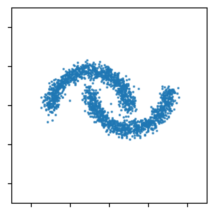
(a) Data samples

(from behavior dataset)

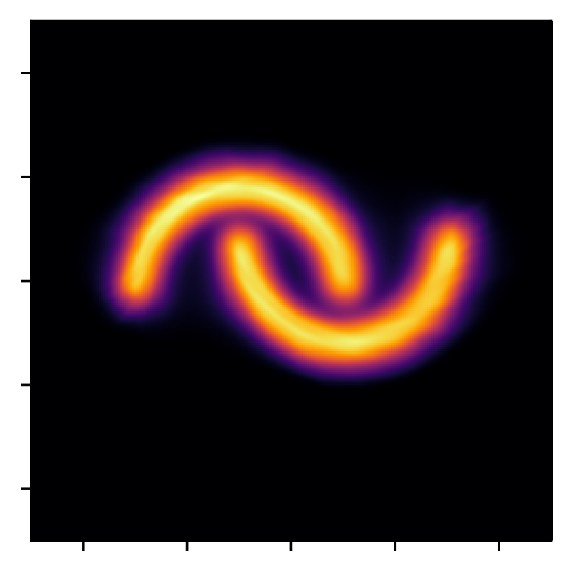
(b) Behavior density $\hat{\mu}({\bm{a}})$

(by diffusion models)

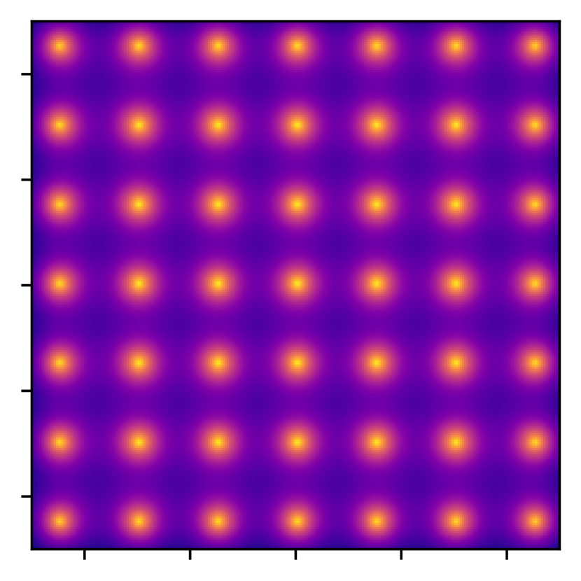
(c) Quadratic Q-functions

(stacked)

(d) Behavior regularization

(${\color[rgb]{0.0,0.0,1.0}\frac{1}{\beta}=0}{\color[rgb]{1,0,0}\longrightarrow}{\color[rgb]{0.0,1.0,0.5}\frac{1}{\beta}=1}$)

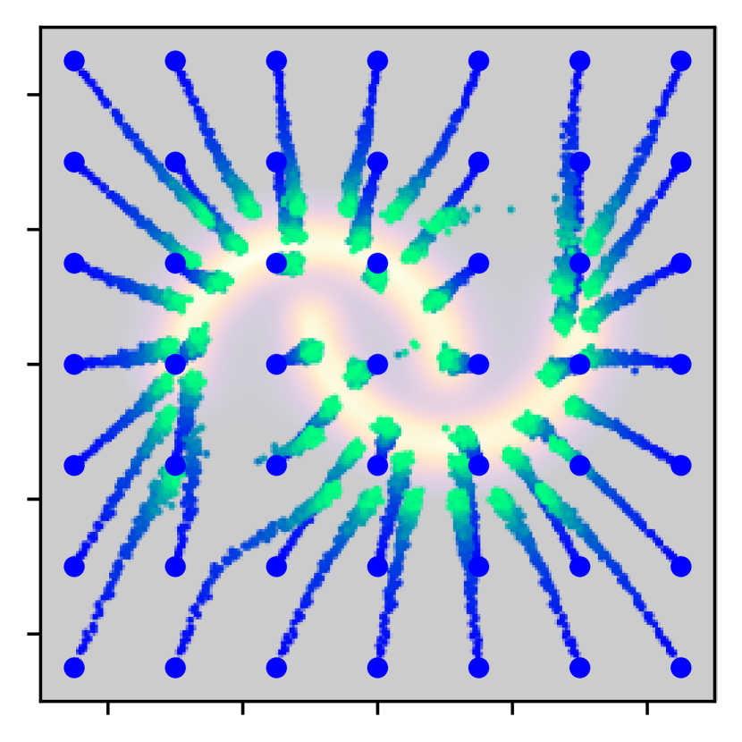
(e) Result policy shift

(by varying $0\leq\frac{1}{\beta}\leq 1$)

Figure 3: Illustration of SRPO in 2D bandit settings. (a) A predefined complex data distribution, which represents the potentially heterogeneous behavior policy $\mu({\bm{a}})$. (b) A diffusion model $\hat{\mu}({\bm{a}})$ is trained to fit the behavior distribution. The data density can be analytically calculated based on Song et al. (2021). (c) The Q-function is manually defined as a quadratic function: $Q({\bm{a}}):=-({\bm{a}}-{\bm{a}}_{\text{tar}})^{2}$, where ${\bm{a}}_{\text{tar}}$ represents the 2D point with the highest estimated Q-value and is selected from a set of grid intersections. These individual Q-functions with different ${\bm{a}}_{\text{tar}}$ are depicted together in a stacked way in Figure (c). (d)&(e) By optimizing deterministic policies $\pi(\cdot)={\bm{a}}_{\text{reg}}$ according to Eq. (10) and tuning the temperature coefficient $\beta$, resulting policies shift from greedy ones which tend to maximize corresponding Q-functions to conservative ones which are successfully constrained close to the behavior distribution. See more experimental results in Appendix A.

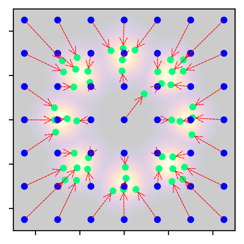
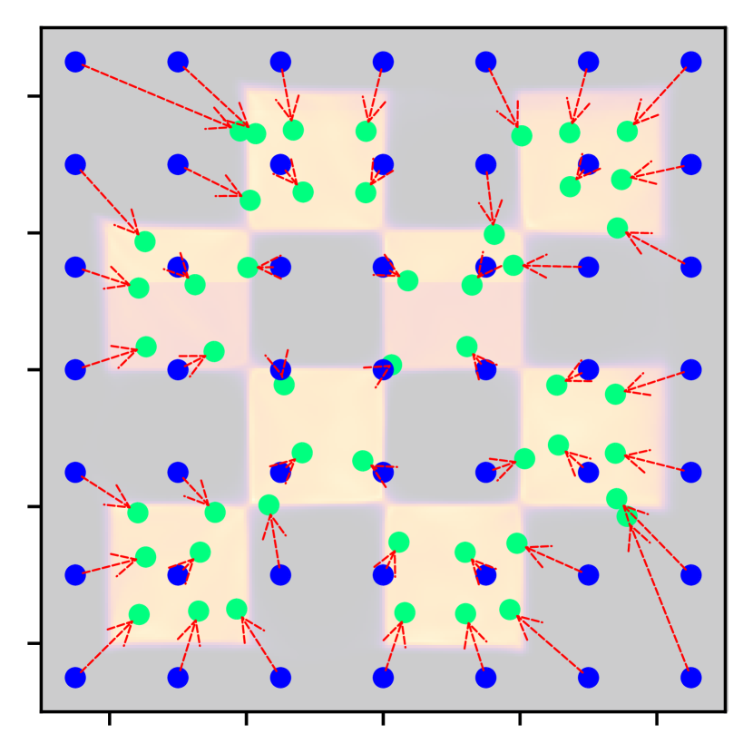
Compared with previous work (Wang et al., 2023a; Lu et al., 2023; Hansen-Estruch et al., 2023) that directly trains a diffusion policy for inference in evaluation, the main advantage of SRPO is its computational efficiency. SRPO entirely circumvents the computationally demanding action sampling scheme associated with the diffusion process. Yet, it still taps into the robust generative strengths of diffusion models, especially their ability to represent potentially diverse behavior datasets.

4 Practical Algorithm

In this section, we derive a practical algorithm for applying SRPO in offline RL (Algorithm 1). The algorithm includes three parts: implicit Q-learning (Section 4.1); diffusion-based behavior modeling (Section 4.1); and score-regularized policy extraction (Section 4.2).

4.1 Pretraining the Diffusion Behavior Model and Q-networks

For Q-networks, we choose to use implicit Q-learning (Kostrikov et al., 2022) to decouple critic training from actor training. The core ingredient of the training pipeline is expectile regression, which requires only sampling actions from existing datasets for bootstrapping:

$$\min_{\zeta}{\mathcal{L}}_{V}(\zeta)=\mathbb{E}_{({\bm{s}},{\bm{a}})\sim\mathcal{D}^{\mu}}[L_{2}^{\tau}(Q_{\phi}({\bm{s}},{\bm{a}})-V_{\zeta}({\bm{s}}))],\mbox{ where }L_{2}^{\tau}({\bm{u}})=|\tau-\mathbbm{1}({\bm{u}}<0)|{\bm{u}}^{2},$$ (11)

$$\min_{\phi}{\mathcal{L}}_{Q}(\phi)=\mathbb{E}_{({\bm{s}},{\bm{a}},{\bm{s}}^{\prime})\sim\mathcal{D}^{\mu}}\left[\|r({\bm{s}},{\bm{a}})+\gamma V_{\zeta}({\bm{s}}^{\prime})-Q_{\phi}({\bm{s}},{\bm{a}})\|_{2}^{2}\right].$$ (12)

When the expectile parameter $\tau\in(0,1)$ is larger than 0.5, the asymmetric L2-objective ${\mathcal{L}}_{V}(\zeta)$ would downweight suboptimal actions which have lower Q-values, removing the need of an explicit policy.

For behavior models, in order to represent the behavior distribution with high fidelity and estimate its score function, we follow previous work (Chen et al., 2023; Hansen-Estruch et al., 2023) and train a conditional behavior cloning model:

$$\min_{\psi}{\mathcal{L}}_{\mu}(\psi)=\mathbb{E}_{t,\bm{\epsilon},({\bm{s}},{\bm{a}})\sim\mathcal{D}^{\mu}}\left[\|\bm{\epsilon}_{\psi}({\bm{a}}_{t}|{\bm{s}},t)-\bm{\epsilon}\|_{2}^{2}\right]_{{\bm{a}}_{t}=\alpha_{t}{\bm{a}}+\sigma_{t}\bm{\epsilon}},$$ (13)

Algorithm 1 SRPO

  Initialize parameters $\psi$, $\zeta$, $\phi$, $\theta$.

   // Critic training (IQL)

  for each gradient step do

     $\zeta\leftarrow\zeta-\lambda_{V}\nabla_{\zeta}L_{V}(\zeta)$ (Eq. 11)

     $\phi\leftarrow\phi-\lambda_{Q}\nabla_{\phi}L_{Q}(\phi)$ (Eq. 12)

   // Behavior training

  for each gradient step do

     $\psi\leftarrow\psi-\lambda_{\mu}\nabla_{\psi}L_{\mu}(\psi)$ (Eq. 13)

   // Policy extraction

  for each gradient step do

     $\theta\leftarrow\theta+\lambda_{\pi}\nabla_{\theta}{\mathcal{L}}^{\text{surr}}_{\pi}(\theta)$ (Eq. 15)

where $t\sim{\mathcal{U}}(0,1)$ and $\bm{\epsilon}\sim{\mathcal{N}}(\bm{0},{\bm{I}})$. The model architecture of $\bm{\epsilon}_{\psi}$ is consistent with the one proposed by Hansen-Estruch et al. (2023), with the sole difference being that our model uses continuous-time inputs similar to Lu et al. (2023) instead of discrete ones as used by Wang et al. (2023a) and Hansen-Estruch et al. (2023).

Once we have finished training the behavior model $\bm{\epsilon}_{\psi}$, we can use it to estimate the score function of $\mu_{t}$, the diffused distribution of $\mu({\bm{a}}|{\bm{s}})$ at time $t$. We have $\nabla_{{\bm{a}}_{t}}\log\mu_{t}({\bm{a}}_{t}|{\bm{s}},t)=-\bm{\epsilon}_{\psi}^{*}({\bm{a}}_{t}|{\bm{s}},t)/\sigma_{t}\approx-\bm{\epsilon}_{\psi}({\bm{a}}_{t}|{\bm{s}},t)/\sigma_{t}$ as shown by Song et al. (2021).

4.2 Policy Extraction from Pretrained Models

The policy extraction scheme proposed in Section 3 only leverages the pretrained diffusion behavior model $\bm{\epsilon}_{\phi}({\bm{a}}_{t}|{\bm{s}},t)$ at time $t\rightarrow 0$, where the behavior distribution $\mu$ has not been diffused. However, $\bm{\epsilon}_{\phi}({\bm{a}}_{t}|{\bm{s}},t)$ is trained to represent a series of diffused behavior distributions $\mu_{t}$ at various times $t\in(0,1)$. In order to exploit the generative capacity of $\bm{\epsilon}_{\phi}$, we replace the original training objective ${\mathcal{L}}_{\pi}(\theta)$ with a new surrogate objective:

$$\max_{\theta}{\mathcal{L}}^{\text{surr}}_{\pi}(\theta)=\mathbb{E}_{{\bm{s}},{\bm{a}}\sim\pi_{\theta}}Q_{\phi}({\bm{s}},{\bm{a}})-\frac{1}{\beta}\mathbb{E}_{t,{\bm{s}}}\omega(t)\frac{\sigma_{t}}{\alpha_{t}}D_{\mathrm{KL}}\left[\pi_{t,\theta}(\cdot|{\bm{s}})||\mu_{t}(\cdot|{\bm{s}})\right],$$ (14)

where $t\sim{\mathcal{U}}(0.02,0.98)$, ${\bm{s}}\sim\mathcal{D}^{\mu}$. Both $\mu_{t}$ and $\pi_{\theta,t}$ follow the same forward diffusion process in Eq. (4), where $\mu_{t}({\bm{a}}_{t}|{\bm{s}}):=\mathbb{E}_{{\bm{a}}\sim\mu(\cdot|{\bm{s}})}{\mathcal{N}}({\bm{a}}_{t}|\alpha_{t}{\bm{a}},\sigma_{t}^{2}{\bm{I}})$, and $\pi_{\theta,t}({\bm{a}}_{t}|{\bm{s}}):=\mathbb{E}_{{\bm{a}}\sim\pi_{\theta}(\cdot|{\bm{s}})}{\mathcal{N}}({\bm{a}}_{t}|\alpha_{t}{\bm{a}},\sigma_{t}^{2}{\bm{I}})$. $\omega(t)$ is a weighting function that adjusts the importance of each time $t$. We can nearly recover ${\mathcal{L}}_{\pi}(\theta)$ by setting $\omega(t)$ to $\delta(t-0.02)\frac{\alpha_{0.02}}{\sigma_{0.02}}$ (ablation studies in Section 6.3).

Empirically, the surrogate objective ${\mathcal{L}}^{\text{surr}}_{\pi}(\theta)$ ensembles various diffused behavior policies $\mu_{t}$ to regularize training of the same parameterized policy $\pi_{\theta}$. This is supported by an observation (Proposition 1 in Appendix B): $\operatorname*{arg\,min}_{\pi}D_{\mathrm{KL}}\left[\pi_{t}(\cdot|{\bm{s}})||\mu_{t}(\cdot|{\bm{s}})\right]=\operatorname*{arg\,min}_{\pi}D_{\mathrm{KL}}\left[\pi(\cdot|{\bm{s}})||\mu(\cdot|{\bm{s}})\right]$.

Similarly to Section 3.2, we can optimize Eq. (14) by calculating its gradient:

Proposition 2.

(Proof in Appendix B) Given that $\pi_{\theta}$ is deterministic (${\bm{a}}=\pi_{\theta}({\bm{s}})$) such that $\pi_{\theta,t}$ is Gaussian (${\bm{a}}_{t}=\alpha_{t}{\bm{a}}+\sigma_{t}\bm{\epsilon}$,  $\bm{\epsilon}\sim{\mathcal{N}}(\bm{0},{\bm{I}})$), the gradient for optimizing $\max{\mathcal{L}}^{\text{surr}}_{\pi}(\theta)$ satisfies

$$\nabla_{\theta}{\mathcal{L}}^{\text{surr}}_{\pi}(\theta)\approx\biggl{[}\mathbb{E}_{{\bm{s}}}\nabla_{{\bm{a}}}Q_{\phi}({\bm{s}},{\bm{a}})|_{{\bm{a}}=\pi_{\theta}({\bm{s}})}-\frac{1}{\beta}\mathbb{E}_{t,{\bm{s}},\bm{\epsilon}}{\color[rgb]{0,0,0}\omega(t)}(\bm{\epsilon}_{\psi}({\bm{a}}_{t}|{\bm{s}},t){\color[rgb]{0,0,1}\underbrace{-\bm{\epsilon}}_{\text{subtracted baseline}}})|_{{\bm{a}}_{t}=\alpha_{t}\pi_{\theta}({\bm{s}})+\sigma_{t}\bm{\epsilon}}\bigg{]}\nabla_{\theta}\pi_{\theta}({\bm{s}}).$$ (15)

Note that we additionally subtract the action noise $\bm{\epsilon}$ from $\bm{\epsilon}_{\psi}({\bm{a}}_{t}|{\bm{s}},t)$ in the above equation. This term does not influence the expected value of $\nabla_{\theta}{\mathcal{L}}^{\text{surr}}_{\pi}(\theta)$ but could reduce the estimation variance since it is correlated with $\bm{\epsilon}_{\psi}({\bm{a}}_{t}|{\bm{s}},t)$ (See Appendix B). We refer to it as the baseline term because it is similar to the subtracted baseline in Policy Gradient (Sutton & Barto, 1998) algorithms.

The idea of ensembling diffused behavior policies for regularization and subtracting the baseline term to reduce estimation variance both draw inspiration from the latest developments in text-to-3D research such as DreamFusion (Poole et al., 2023). We elaborate more on the connection between the two work in Section 5 and ablate these techniques in the realm of continuous control in Section 6.3.

5 Related Work

Behavior Regularization in Offline Reinforcement Learning.

Behavior regularization can be achieved either implicitly or explicitly. Explicit methods usually necessitate the construction of a behavior model to regularize the learned policy. For example, TD3+BC (Fujimoto & Gu, 2021) implicitly views the behavior as Gaussians and introduces an auxiliary L2-loss term to realize the regularization. SBAC (Xu et al., 2021) and Fisher-BRC (Kostrikov et al., 2021) leverage explicit Gaussian (mixture) behavior models for density estimation of the behavior distribution and guide the learned policy towards areas of high behavior density. BCQ (Fujimoto et al., 2019) and BEAR (Kumar et al., 2019) represent the behavior policy using VAE models (Kingma & Welling, 2014). BCQ limits the action space within the latent domain of a trained VAE-based behavior model, while BEAR employs sample-based MMD kernel (Gretton et al., 2007) to approximate the divergence between the learned and the behavior policy. Diffusion-QL (Wang et al., 2023a) is similar to TD3+BC but swaps the auxiliary loss with a diffusion-centric objective (Ho et al., 2020). QGPO (Lu et al., 2023) views a pretrained diffusion behavior as the Bayesian prior in energy-guided diffusion sampling.

Diffusion Models in Offline Reinforcement Learning.

Recent advancements in offline RL have identified diffusion models as an impactful tool. A primary strength of diffusion modeling lies in its robust generative capability, combined with a straightforward training pipeline, as has been evidenced across numerous research domains (Dhariwal & Nichol, 2021; Xu et al., 2022; Poole et al., 2023). This renders it particularly suitable for modeling heterogeneous behavior datasets (Janner et al., 2022; Wang et al., 2023a; Ajay et al., 2023; Hansen-Estruch et al., 2023), generating in-support actions for Q-learning (Goo & Niekum, 2022; Lu et al., 2023), and representing multimodal policies (Chen et al., 2023; Pearce et al., 2022).

However, a significant concern for integrating diffusion models into RL is the considerable time taken for sampling. Various strategies have been proposed to address this challenge, including employing a parallel sampling scheme during both training and evaluation (Chen et al., 2023), utilizing a specialized diffusion ODE solver such as DPM-solver (Lu et al., 2022; 2023), adopting an approximate diffusion sampling scheme to minimize sampling steps required (Kang et al., 2023), and crafting high-throughput network architectures (Hansen-Estruch et al., 2023). While these techniques offer improvements, they don’t entirely eliminate the need for iterative sampling.

Score Distillation Methods.

Recent developments in text-to-3D generation have enabled the transformation of textual information into 3D content without requiring any 3D training data (Poole et al., 2023; Wang et al., 2023b). This is realized by distilling knowledge from text-to-image diffusion models. A representative method in this domain is DreamFusion (Poole et al., 2023). It optimizes a 3D NeRF model (Mildenhall et al., 2021) by ensuring its projected 2D gradient follows the score direction of a large-scale, pretrained 2D diffusion model (Saharia et al., 2022). Similar to DreamFusion, SRPO also employs a diffusion model to guide the training of a subsequent network. However, our method emphasizes score regularization as opposed to score distillation. The behavior score is additionally incorporated to regularize the Q-gradient instead of being the only supervising signal.

6 Evaluation

6.1 D4RL Performance

Dataset	Environment	BEAR	TD3+BC	IQL	SfBC	Diffuser	Diffusion-QL	QGPO	IDQL	SRPO (Ours)
Medium-Expert	HalfCheetah	$53.4$	$90.7$	$86.7$	$\bf{92.6}$	$79.8$	$\bf{96.8}$	$\bf{93.5}$	$\bf{95.9}$	$\bf{92.2\pm 3.0}$
Medium-Expert	Hopper	$96.3$	$98.0$	$91.5$	$\bf{108.6}$	$\bf{107.2}$	$\bf{111.1}$	$\bf{108.0}$	$\bf{108.6}$	$100.1\pm 13.9$
Medium-Expert	Walker2d	$40.1$	$\bf{110.1}$	$\bf{109.6}$	$\bf{109.8}$	$\bf{108.4}$	$\bf{110.1}$	$\bf{110.7}$	$\bf{112.7}$	$\bf{114.0\pm 2.1}$
Medium	HalfCheetah	$41.7$	$48.3$	$47.4$	$45.9$	$44.2$	$51.1$	$54.1$	$51.0$	$\bf{60.4\pm 0.8}$
Medium	Hopper	$52.1$	$59.3$	$66.3$	$57.1$	$58.5$	$90.5$	$\bf{98.0}$	$65.4$	$\bf{95.5\pm 2.0}$
Medium	Walker2d	$59.1$	$\bf{83.7}$	$78.3$	$77.9$	$79.7$	$\bf{87.0}$	$\bf{86.0}$	$82.5$	$\bf{84.4\pm 4.4}$
Medium-Replay	HalfCheetah	$38.6$	$44.6$	$44.2$	$37.1$	$42.2$	$47.8$	$47.6$	$45.9$	$\bf{51.4\pm 3.4}$
Medium-Replay	Hopper	$33.7$	$60.9$	$94.7$	$86.2$	$\bf{101.3}$	$\bf{100.7}$	$\bf{96.9}$	$92.1$	$\bf{101.2\pm 1.0}$
Medium-Replay	Walker2d	$19.2$	$81.8$	$73.9$	$65.1$	$61.2$	$\bf{95.5}$	$84.4$	$85.1$	$84.6\pm 7.1$
Average (Locomotion)		$51.9$	$75.3$	$76.9$	$75.6$	$75.3$	$\bf{88.0}$	$\bf{86.6}$	$82.1$	$\bf{87.1}$
Default	AntMaze-umaze	$73.0$	$78.6$	$87.5$	$92.0$	-	$93.4$	$\bf{96.4}$	$\bf{94.0}$	$\bf{97.1\pm 2.7}$
Diverse	AntMaze-umaze	$61.0$	$71.4$	$62.2$	$\bf{85.3}$	-	$66.2$	$74.4$	$80.2$	$\bf{82.1\pm 10.8}$
Play	AntMaze-medium	$0.0$	$10.6$	$71.2$	$\bf{81.3}$	-	$76.6$	$\bf{83.6}$	$\bf{84.5}$	$\bf{80.7\pm 7.1}$
Diverse	AntMaze-medium	$8.0$	$3.0$	$70.0$	$\bf{82.0}$	-	$78.6$	$\bf{83.8}$	$\bf{84.8}$	$75.0\pm 12.3$
Play	AntMaze-large	$0.0$	$0.2$	$39.6$	$59.3$	-	$46.4$	$\bf{66.6}$	$\bf{63.5}$	$53.6\pm 12.5$
Diverse	AntMaze-large	$0.0$	$0.0$	$47.5$	$45.5$	-	$56.6$	$\bf{64.8}$	$\bf{67.9}$	$53.6\pm 6.3$
Average (AntMaze)		$23.7$	$27.3$	$63.0$	$74.2$	-	$69.6$	$\bf{78.3}$	$\bf{79.1}$	$73.6$

Table 1: Evaluation numbers of D4RL benchmarks (normalized as suggested by Fu et al. (2020)). We report mean ± standard deviation of algorithm performance across 6 random seeds at the end of training. Numbers within 5 % of the maximum in every individual task are highlighted.

In Table 1, we evaluate the D4RL performance (Fu et al., 2020) of SRPO against other offline RL algorithms. Our chosen benchmarks include conventional methods like BEAR (Kumar et al., 2019), TD3+BC (Fujimoto & Gu, 2021), and IQL (Kostrikov et al., 2022), which feature extracting a Gaussian/Dirac policy for evaluation. We also look at newer diffusion-based offline RL techniques, such as Diffuser (Janner et al., 2022), DIffusion-QL (Wang et al., 2023a), SfBC (Chen et al., 2023), QGPO (Lu et al., 2023), and DIQL (Hansen-Estruch et al., 2023). These methods tend to be more computationally intensive but generally offer better results.

Of all the baselines, our comparison with DIQL is particularly informative. This is because SRPO shares a virtually identical training pipeline and model architecture for critic and behavior models with DIQL, as is deliberately crafted. The most significant distinction lies in their approaches for extracting policy: DIQL skips the policy extraction step, choosing to evaluate directly with the behavior policy, using a selecting-from-behavior-candidates technique (Chen et al., 2023). In contrast, SRPO extracts a Dirac policy from behavior and critic models.

Figure 4: Training curves of SRPO (ours) and several baselines. See complete experimental results in Appendix D.

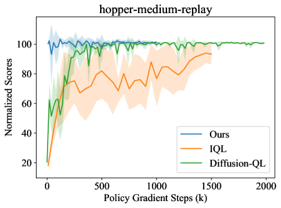
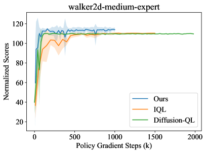
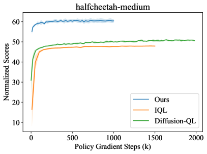
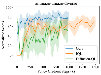
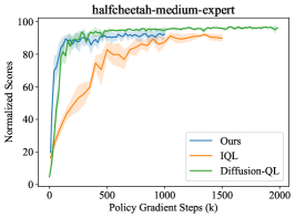
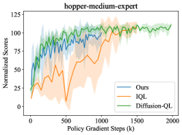
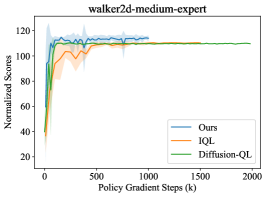
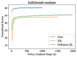
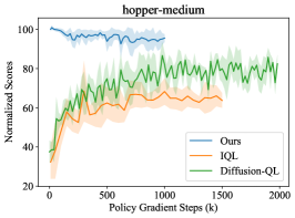
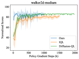
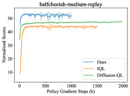
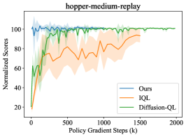
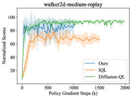
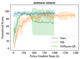
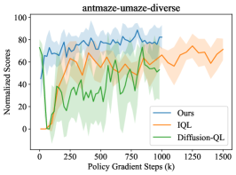
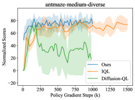
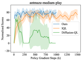
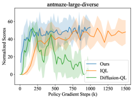
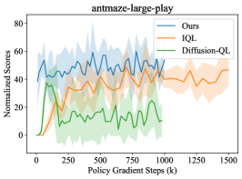
Overall, SRPO consistently surpasses referenced baselines that also utilize a Gaussian (or Dirac) inference policy, leading by large margins in the majority of tasks. It also comes close to matching the benchmarks set by other state-of-the-art diffusion-based methods, such as Diffusion-QL and IDQL, though it features a much simpler inference policy. Moreover, in the case of the convergence rate and training stability, we showcase training plots of SRPO alongside several baselines in Figure 4. Results also suggest that compared with both weighted regression methods like IQL and reverse-KL-based optimization strategies like Diffusion-QL, SRPO exhibits more favorable attributes. We attribute the performance gain of SRPO to the utilization of diffusion behavior modeling, which facilitates a more effective realization of the training formulation.

6.2 Computational Efficiency

Figure 5: Training and inference (evaluation) time required for different algorithms in D4RL locomotion tasks. All experiments are conducted with the same PyTorch backend and the same computing hardware setup.

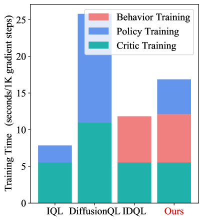
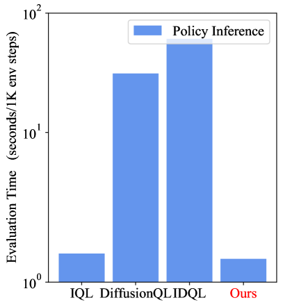
As indicated by Figure 1 and 5, SRPO maintains high computational efficiency, especially fast inference speed, while enabling the use of a powerful diffusion model. Notably, the action sampling speed of SRPO is 25 to 1000 times faster than that of other diffusion-based methods. Additionally, its computational FLOPS amount to only 0.25% to 0.01% of other methods. This makes SRPO ideal for computation-sensitive contexts such as robotics. It also speeds up experimentation, since policy evaluation typically consumes over half of the experiment duration for previous diffusion-based approaches. This efficiency stems from SRPO’s design, which completely avoids diffusion sampling throughout both training and evaluation procedures.

6.3 Ablation Studies

Figure 6: Ablation for implementation details of Eq. (15). All results are averaged under 6 random seeds.

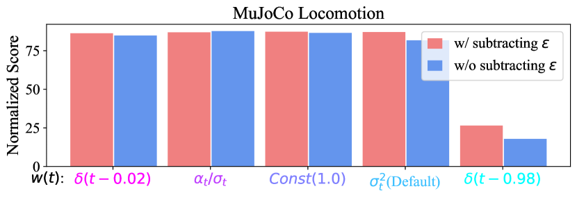
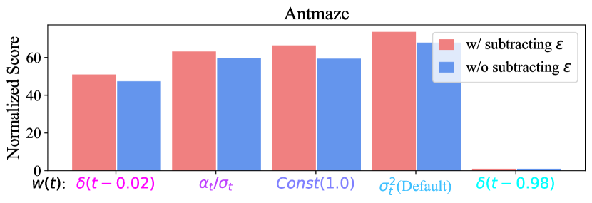
Weighting function $\omega(t)$.

As is explained in Section 4.2, if $\omega(t)\propto\delta(t-0.02)$, the surrogate objective nearly recovers the original one, which could guarantee convergence to the wanted optimal policy $\pi^{*}$. Adjusting $\omega(t)$ to ensemble diffused behavior score at various times $t\in(0,1)$ might yield a smoother and more robust gradient landscape. However, it biases the original training objective. In an extreme case where $\omega(t)\propto\delta(t-0.98)$, the estimated behavior score almost becomes the score function of pure Gaussian distribution, making it entirely helpless. From Figure 6, we empirically observe that Antmaze tasks are sensitive to variation of $\omega(t)$, while Locomotion tasks are not. Overall, we find $\omega(t)=\sigma_{t}^{2}$ is a suitable choice for all tested tasks and choose it as the default hyperparameter throughout our experiments. This hyperparameter choice is consistent with previous literature (Poole et al., 2023).

Subtracting baselines $\bm{\epsilon}$.

In Figure 6, we show that subtracting baselines $\bm{\epsilon}$ from the estimated behavior gradient, as is described in Eq. (15), consistently offers slightly better performance.

Temperature coefficient $\beta$ and others.

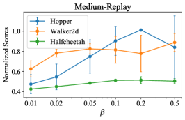
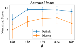
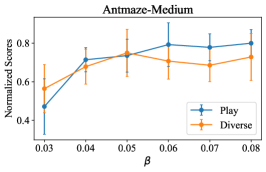
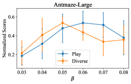
Varying $\beta$ directly controls the conservativness of policy, and thus influences the performance. Experimental results with respect to $\beta$ and other implementation choices are presented in Appendix C.

7 Conclusion

In this paper, we introduce Score Regularized Policy Optimization (SRPO), an innovative offline RL algorithm harnessing the capabilities of diffusion models while circumventing the time-consuming diffusion sampling scheme. SRPO tackles the behavior-regularized policy optimization problem and provides a computationally efficient way to realize behavior regularization through diffusion behavior modeling. The fusion of SRPO with techniques like implicit Q-learning can further solidify its application in computationally sensitive domains, such as robotics.

Appendix A More 2D Results

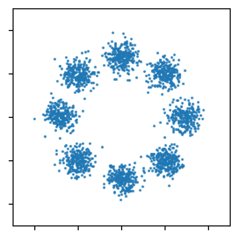
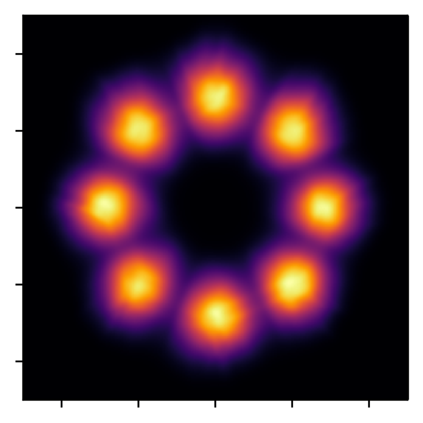
8gaussians

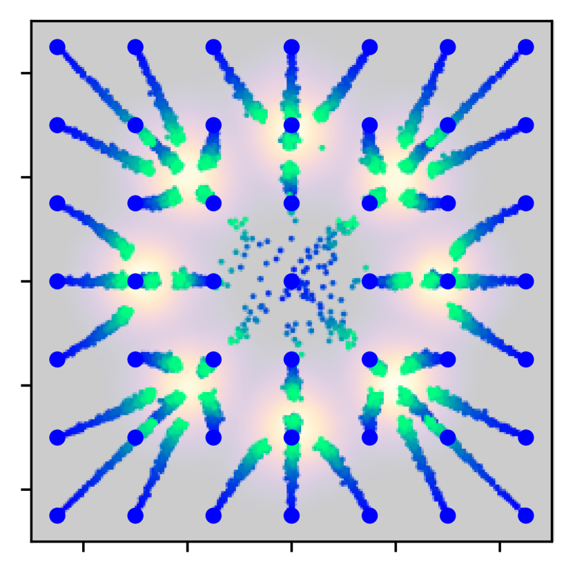
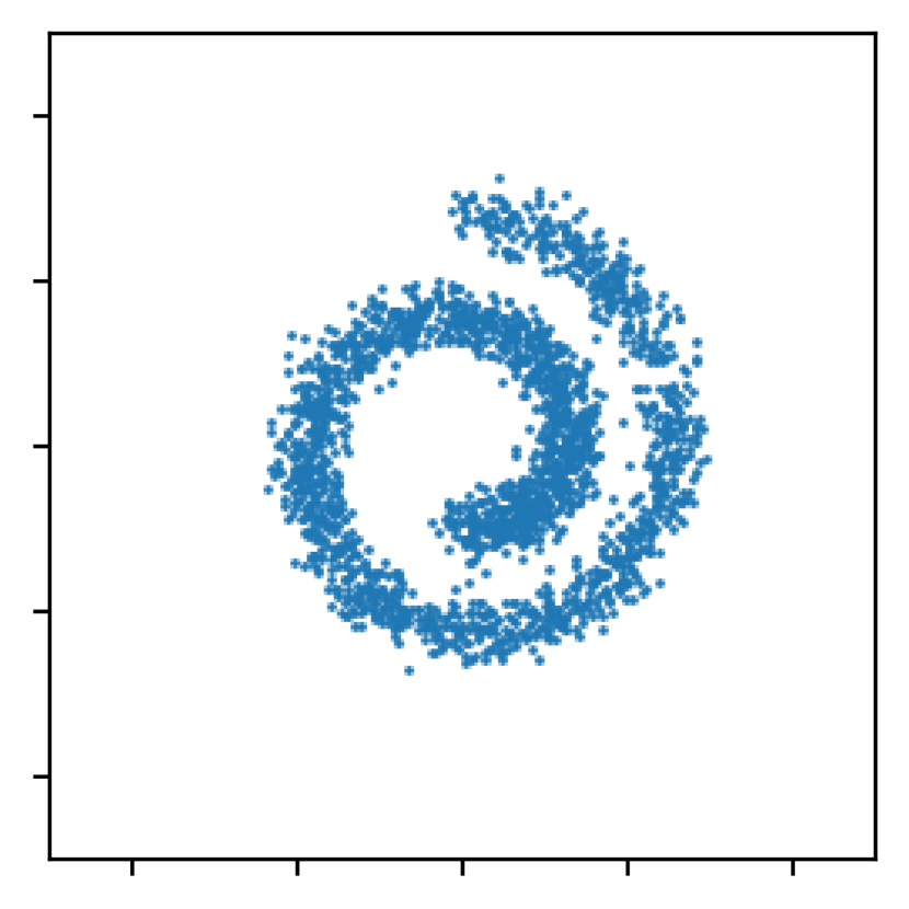
swissroll

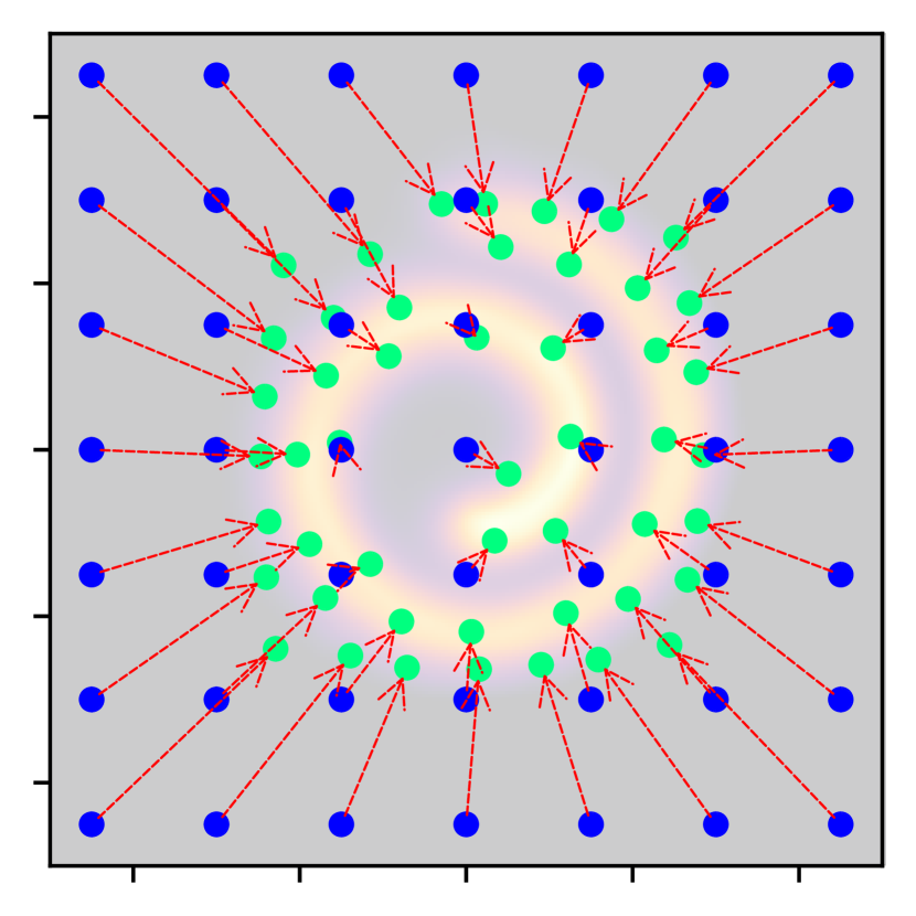
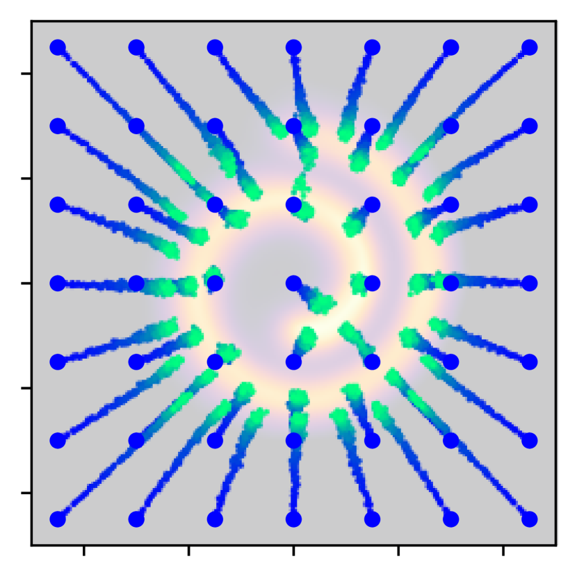
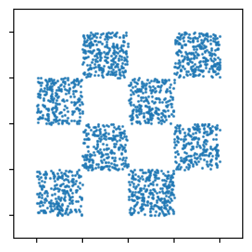
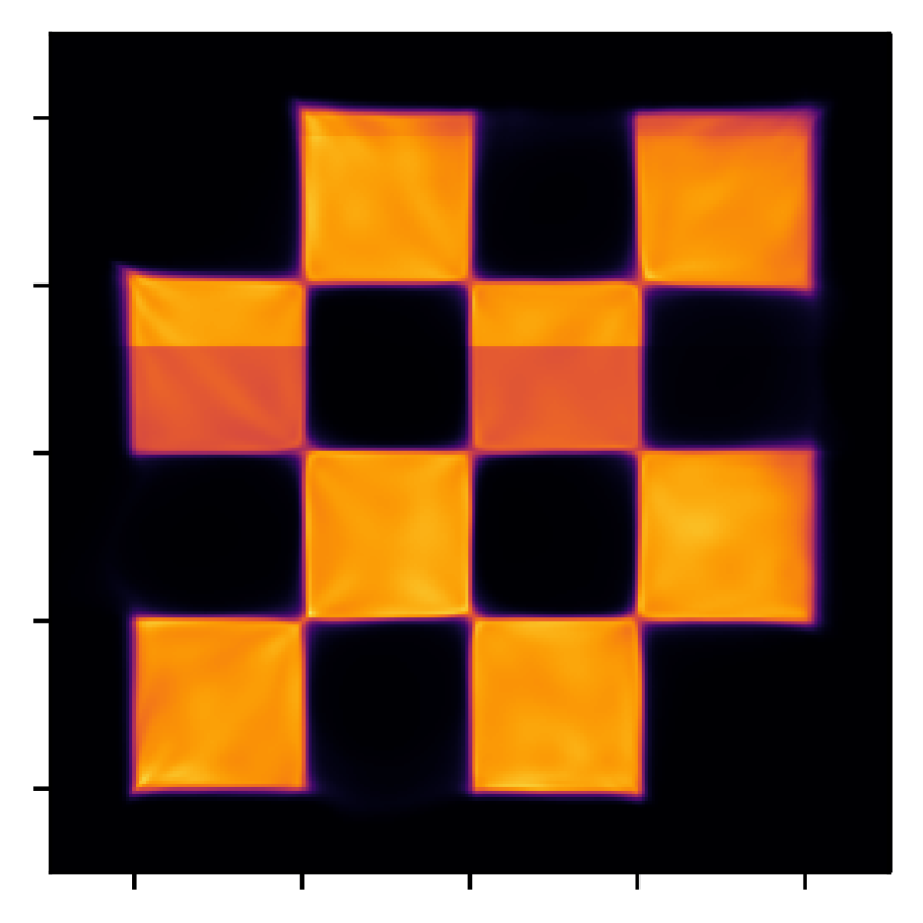
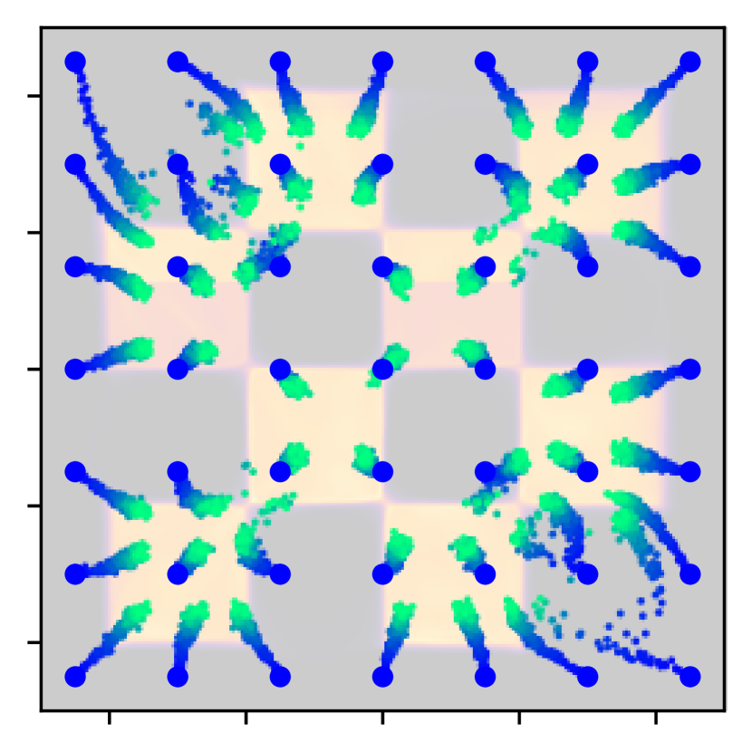
checkboard

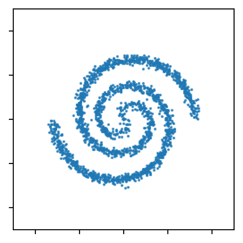
2spirals

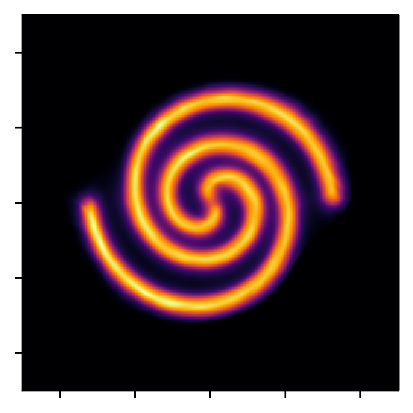
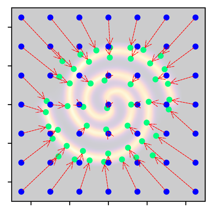
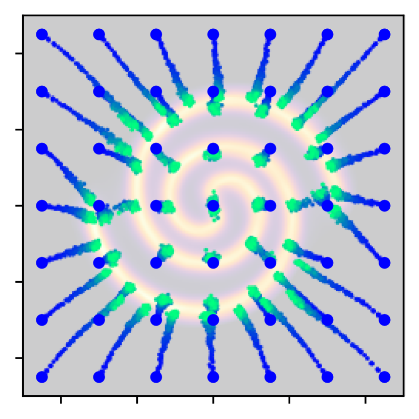
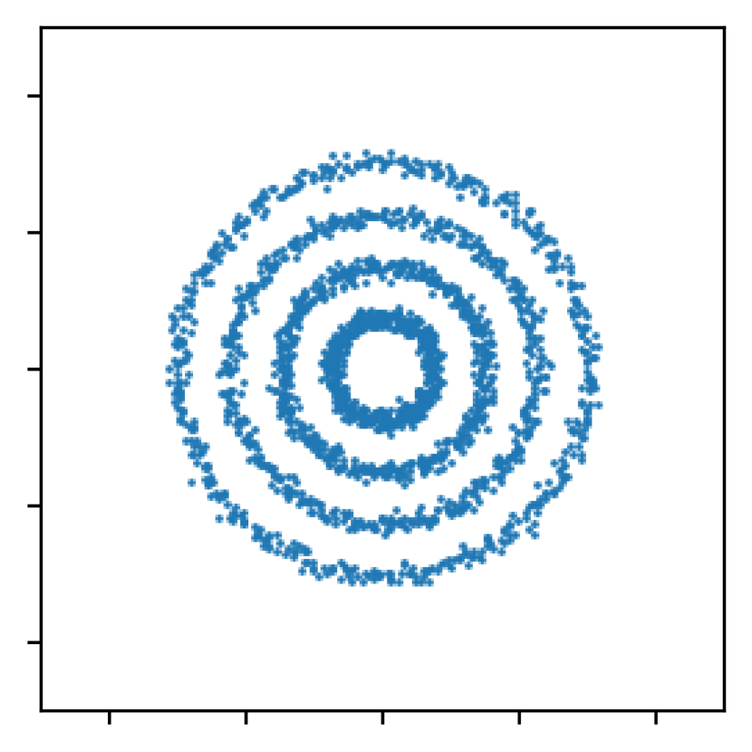
rings

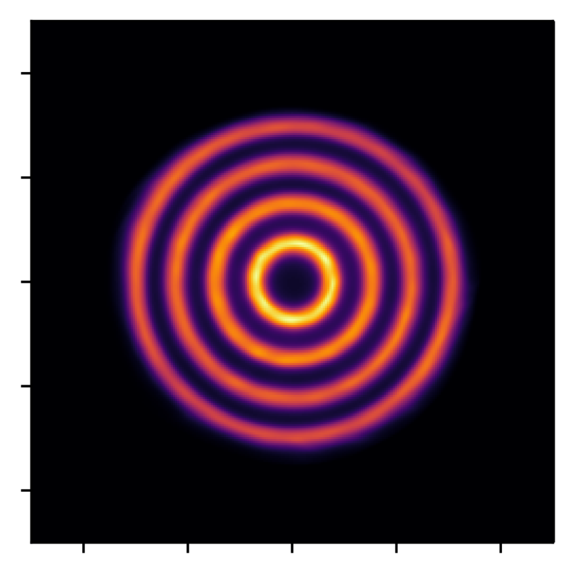
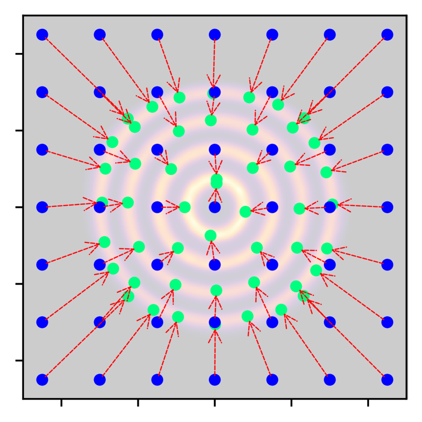
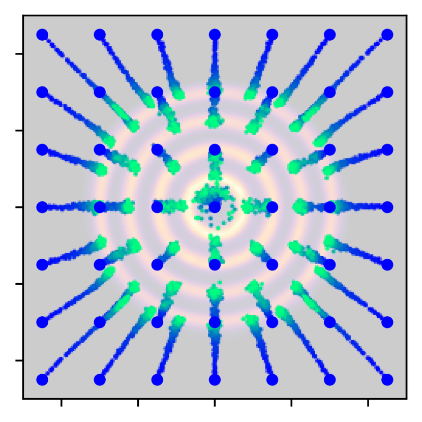
Data samples

(from behavior dataset)

moons

Behavior density $\hat{\mu}({\bm{a}})$

(by diffusion models)

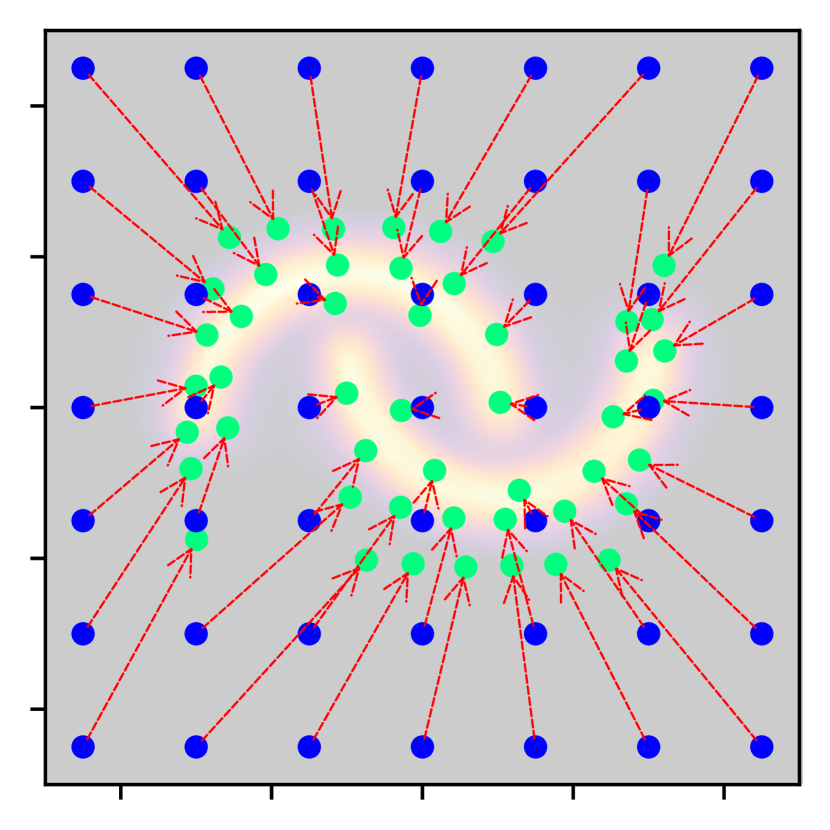
Behavior regularization

(${\color[rgb]{0.0,0.0,1.0}\frac{1}{\beta}=0}{\color[rgb]{1,0,0}\longrightarrow}{\color[rgb]{0.0,1.0,0.5}\frac{1}{\beta}=1}$)

Result policy shift

(by varying $0\leq\frac{1}{\beta}\leq 1$)

Figure 7: Experimental results of SRPO in 2D bandit settings.

Appendix B Theoretical Analysis

In this section, we provide some theoretical analysis related to the SPRO algorithm.

First, we aim to provide some insights into why it is reasonable to replace

$${\mathcal{L}}_{\pi}(\theta)=\mathbb{E}_{{\bm{s}}\sim\mathcal{D}^{\mu},{\bm{a}}\sim\pi_{\theta}}Q_{\phi}({\bm{s}},{\bm{a}})-\frac{1}{\beta}{\color[rgb]{0,0,1}D_{\mathrm{KL}}\left[\pi_{\theta}(\cdot|{\bm{s}})||\mu(\cdot|{\bm{s}})\right]}$$

with the surrogate objective

$${\mathcal{L}}^{\text{surr}}_{\pi}(\theta)=\mathbb{E}_{{\bm{s}},{\bm{a}}\sim\pi_{\theta}}Q_{\phi}({\bm{s}},{\bm{a}})-\frac{1}{\beta}\mathbb{E}_{t,{\bm{s}}}\omega(t)\frac{\sigma_{t}}{\alpha_{t}}{\color[rgb]{0,0,1}D_{\mathrm{KL}}\left[\pi_{t,\theta}(\cdot|{\bm{s}})||\mu_{t}(\cdot|{\bm{s}})\right]}.$$ (16)

Proposition 1.

Given that $\pi$ is sufficiently expressive, for any time $t$, any state ${\bm{s}}$, we have

$$\operatorname*{arg\,min}_{\pi}D_{\mathrm{KL}}\left[\pi_{t}(\cdot|{\bm{s}})||\mu_{t}(\cdot|{\bm{s}})\right]=\operatorname*{arg\,min}_{\pi}D_{\mathrm{KL}}\left[\pi(\cdot|{\bm{s}})||\mu(\cdot|{\bm{s}})\right],$$

where both $\mu_{t}$ and $\pi_{t}$ follow the same predefined diffusion process in Eq. (4).

Proof.

Our proof is inspired by Wang et al. (2023b). Regarding the property of the KL divergence, we have $\operatorname*{arg\,min}_{\pi}D_{\mathrm{KL}}\left[\pi(\cdot|{\bm{s}})||\mu(\cdot|{\bm{s}})\right]=\mu(\cdot|{\bm{s}})$ and $\pi_{t}^{*}(\cdot|{\bm{s}}):=\operatorname*{arg\,min}_{\pi}D_{\mathrm{KL}}\left[\pi_{t}(\cdot|{\bm{s}})||\mu_{t}(\cdot|{\bm{s}})\right]=\mu_{t}(\cdot|{\bm{s}})$.

We conclude that $\pi_{t}^{*}(\cdot|{\bm{s}})=\mu_{t}(\cdot|{\bm{s}})$ is equivalent to $\pi^{*}(\cdot|{\bm{s}})=\mu(\cdot|{\bm{s}})$ by transforming all distributions into their characteristic functions.

According to the forward diffusion process defined by Eq. (4), for any prespecified state ${\bm{s}}$, we have

$${\bm{a}}_{t}^{\pi}=\alpha_{t}{\bm{a}}_{0}^{\pi}+\sigma_{t}\epsilon=\alpha_{t}{\bm{a}}^{\pi}+\sigma_{t}\epsilon,$$

such that

$$\pi_{t}({\bm{a}}_{t}|{\bm{s}})=\int{\mathcal{N}}({\bm{a}}_{t}|\alpha_{t}{\bm{a}},\sigma_{t}^{2}{\bm{I}})\pi({\bm{a}}|{\bm{s}})\mathrm{d}{\bm{a}},$$

Therefore, the characteristic function of $\pi_{t}({\bm{a}}_{t}|{\bm{s}})$ satisfies

$$\phi_{\pi_{t}(\cdot|{\bm{s}})}(u)=\phi_{\pi(\cdot|{\bm{s}})}(\alpha_{t}u)\phi_{{\mathcal{N}}(\mathbf{0},{\bm{I}})}(\sigma_{t}u)=\phi_{\pi(\cdot|{\bm{s}})}(\alpha_{t}s)e^{-\frac{\sigma_{t}^{2}u^{2}}{2}}.$$

Similarly, we also have

$$\phi_{\mu_{t}(\cdot|{\bm{s}})}(u)=\phi_{\mu(\cdot|{\bm{s}})}(\alpha_{t}u)\phi_{{\mathcal{N}}(\mathbf{0},{\bm{I}})}(\sigma_{t}u)=\phi_{\mu(\cdot|{\bm{s}})}(\alpha_{t}s)e^{-\frac{\sigma_{t}^{2}u^{2}}{2}}.$$

Finally, we can see that

$$\pi_{t}^{*}(\cdot|{\bm{s}})=\mu_{t}(\cdot|{\bm{s}})\Leftrightarrow\phi_{\pi^{*}_{t}(\cdot|{\bm{s}})}(u)=\phi_{\mu_{t}(\cdot|{\bm{s}})}(u)\Leftrightarrow\phi_{\pi^{*}(\cdot|{\bm{s}})}(u)=\phi_{\mu(\cdot|{\bm{s}})}(u)\Leftrightarrow\pi^{*}(\cdot|{\bm{s}})=\mu(\cdot|{\bm{s}})$$

∎

Remark 1.

It is imperative to note that although $\operatorname*{arg\,min}_{\pi}D_{\mathrm{KL}}\left[\pi_{t}(\cdot|{\bm{s}})||\mu_{t}(\cdot|{\bm{s}})\right]$ and $\operatorname*{arg\,min}_{\pi}D_{\mathrm{KL}}\left[\pi(\cdot|{\bm{s}})||\mu(\cdot|{\bm{s}})\right]$ converge to the same global optimal solution. $\max{\mathcal{L}}^{\text{surr}}_{\pi}(\theta)$ does not converge to the wanted optimal policy $\pi^{*}({\bm{a}}|{\bm{s}})\propto\mu({\bm{a}}|{\bm{s}})\ \mathrm{exp}\left(\beta Q_{\phi}({\bm{s}},{\bm{a}})\right)$ while $\max{\mathcal{L}}_{\pi}(\theta)$ does. This discrepancy arises primarily from the inclusion of the additional Q-function term. Furthermore, in practical scenarios, the parameterized policy $\pi_{\theta}$ lacks expressivity, which hinders its ability to truly attain the global optimum. Nevertheless, ensembling a series of $t$ might be beneficial for the optimization to get to a better minimum in practice. Since the distribution $\mu(\cdot|{\bm{s}})$ is usually complex and high-dimensional, it is easy to become trapped in a local minimum while maximizing its likelihood. However, the distribution of $\mu_{t}(\cdot|{\bm{s}})$ gets smoother as $t$ gets larger.

Next, we derive the gradient for ${\mathcal{L}}^{\text{surr}}_{\pi}(\theta)$ under the condition that $\pi_{\theta}$ is a deterministic actor.

Proposition 2.

Given that $\pi_{\theta}$ is a deterministic actor (${\bm{a}}=\pi_{\theta}({\bm{s}})$) and $\bm{\epsilon}^{*}$ is an optimal diffusion behavior model ($\bm{\epsilon}^{*}({\bm{a}}_{t}|{\bm{s}},t)=-\sigma_{t}\nabla_{{\bm{a}}_{t}}\log\mu_{t}({\bm{a}}_{t}|{\bm{s}})$), the gradient for optimizing $\max_{\theta}{\mathcal{L}}^{\text{surr}}_{\pi}(\theta)$ in Eq. (16) satisfies

$$\nabla_{\theta}{\mathcal{L}}^{\text{surr}}_{\pi}(\theta)=\left[\mathbb{E}_{{\bm{s}}}\nabla_{{\bm{a}}}Q_{\phi}({\bm{s}},{\bm{a}})|_{{\bm{a}}=\pi_{\theta}({\bm{s}})}-\frac{1}{\beta}\mathbb{E}_{t,{\bm{s}},\bm{\epsilon}}{\color[rgb]{0,0,0}\omega(t)}(\bm{\epsilon}^{*}({\bm{a}}_{t}|{\bm{s}},t){\color[rgb]{0,0,0}-\bm{\epsilon}})|_{{\bm{a}}_{t}=\alpha_{t}\pi_{\theta}({\bm{s}})+\sigma_{t}\bm{\epsilon}}\right]\nabla_{\theta}\pi_{\theta}({\bm{s}})$$

Proof.

According to the predefined forward diffusion process (Eq. (4)), for any state ${\bm{s}}$, we have

$$\pi_{\theta,t}({\bm{a}}_{t}|{\bm{s}})=\int{\mathcal{N}}({\bm{a}}_{t}|\alpha_{t}{\bm{a}},\sigma_{t}^{2}{\bm{I}})\pi_{\theta}({\bm{a}}|{\bm{s}})\mathrm{d}{\bm{a}}=\int{\mathcal{N}}({\bm{a}}_{t}|\alpha_{t}{\bm{a}},\sigma_{t}^{2}{\bm{I}})\delta({\bm{a}}-\pi_{\theta}({\bm{s}}))\mathrm{d}{\bm{a}}={\mathcal{N}}({\bm{a}}_{t}|\alpha_{t}\pi_{\theta}({\bm{s}}),\sigma_{t}^{2}{\bm{I}}).$$

Therefore $\pi_{\theta,t}(\cdot|{\bm{s}})$ is a Gaussian with expected value $\alpha_{t}\pi_{\theta}({\bm{s}})$ and variance $\sigma_{t}^{2}{\bm{I}}$. We rewrite the training objective below:

$${\mathcal{L}}^{\text{surr}}_{\pi}(\theta) =\mathbb{E}_{{\bm{s}},{\bm{a}}\sim\pi_{\theta}(\cdot|{\bm{s}})}Q_{\phi}({\bm{s}},{\bm{a}})-\frac{1}{\beta}\mathbb{E}_{t,{\bm{s}}}\omega(t)\frac{\sigma_{t}}{\alpha_{t}}D_{\mathrm{KL}}\left[\pi_{t,\theta}(\cdot|{\bm{s}})||\mu_{t}(\cdot|{\bm{s}})\right]$$

$$=\mathbb{E}_{{\bm{s}},{\bm{a}}\sim\pi_{\theta}(\cdot|{\bm{s}})}Q_{\phi}({\bm{s}},{\bm{a}})+\frac{1}{\beta}\mathbb{E}_{t,{\bm{s}},{\bm{a}}_{t}\sim\pi_{t,\theta}(\cdot|{\bm{s}})}\omega(t)\frac{\sigma_{t}}{\alpha_{t}}[\log\mu_{t}({\bm{a}}_{t}|{\bm{s}})-\log\pi_{t,\theta}({\bm{a}}_{t}|{\bm{s}})]$$

$$=\mathbb{E}_{{\bm{s}}}Q_{\phi}({\bm{s}},{\bm{a}})|_{{\bm{a}}=\pi_{\theta}({\bm{s}})}+\frac{1}{\beta}\mathbb{E}_{t,{\bm{s}}}\omega(t)\frac{\sigma_{t}}{\alpha_{t}}\mathbb{E}_{{\bm{a}}_{t}\sim{\mathcal{N}}(\cdot|\alpha_{t}\pi_{\theta}({\bm{s}}),\sigma_{t}^{2}{\bm{I}})}[\log\mu_{t}({\bm{a}}_{t}|{\bm{s}})-\log\pi_{t,\theta}({\bm{a}}_{t}|{\bm{s}})]$$

Then we derive the gradient of ${\mathcal{L}}^{\text{surr}}_{\pi}(\theta)$ by applying the chain rule and the parameterization trick:

$$\nabla_{\theta}{\mathcal{L}}^{\text{surr}}_{\pi}(\theta)= \frac{\partial\mathbb{E}_{{\bm{s}}}Q_{\phi}({\bm{s}},{\bm{a}})}{\partial{\bm{a}}}|_{{\bm{a}}=\pi_{\theta}({\bm{s}})}\frac{\partial\pi_{\theta}({\bm{s}})}{\partial\theta}+\frac{1}{\beta}\mathbb{E}_{t,{\bm{s}}}\omega(t)\frac{\sigma_{t}}{\alpha_{t}}\mathbb{E}_{\epsilon}\underbrace{\frac{\partial[\log\mu_{t}({\bm{a}}_{t}|{\bm{s}})]}{\partial{\bm{a}}_{t}}}_{\text{behavior score}}\frac{\partial{\bm{a}}_{t}}{\partial\theta}|_{{\bm{a}}_{t}=\alpha_{t}\pi_{\theta}({\bm{s}})+\sigma_{t}\epsilon}$$

$$-\frac{1}{\beta}\mathbb{E}_{t,{\bm{s}}}\omega(t)\frac{\sigma_{t}}{\alpha_{t}}\biggl{[}\mathbb{E}_{\epsilon}\underbrace{\frac{\partial[\log\pi_{t,\theta}({\bm{a}}_{t}|{\bm{s}})]}{\partial{\bm{a}}_{t}}}_{\text{policy score}}\frac{\partial{\bm{a}}_{t}}{\partial\theta}|_{{\bm{a}}_{t}=\alpha_{t}\pi_{\theta}({\bm{s}})+\sigma_{t}\epsilon}+\underbrace{\mathbb{E}_{{\bm{a}}_{t}\sim\pi_{t,\theta}(\cdot|{\bm{s}})}\frac{\partial\log\pi_{t,\theta}({\bm{a}}_{t}|{\bm{s}})}{\partial\theta}}_{\text{parameter score}}\biggr{]}$$ (17)

The behavior score term in the above equation can be represented by the optimal diffusion behavior model:

$$\frac{\partial[\log\mu_{t}({\bm{a}}_{t}|{\bm{s}})]}{\partial{\bm{a}}_{t}}=-\frac{\bm{\epsilon}^{*}({\bm{a}}_{t}|{\bm{s}},t)}{\sigma_{t}}.$$

The policy score term is the score function of $\pi_{t,\theta}(\cdot|{\bm{s}})={\mathcal{N}}(\alpha_{t}\pi_{\theta}({\bm{s}}),\sigma_{t}^{2}{\bm{I}})$, we have

$$\frac{\partial[\log\pi_{t,\theta}({\bm{a}}_{t}|{\bm{s}})]}{\partial{\bm{a}}_{t}}=-\frac{\partial}{\partial{\bm{a}}_{t}}\frac{\|{\bm{a}}_{t}-\alpha_{t}\pi_{\theta}({\bm{s}})\|_{2}^{2}}{2\sigma_{t}^{2}}|_{{\bm{a}}_{t}=\alpha_{t}\pi_{\theta}({\bm{s}})}=\frac{\epsilon}{\sigma_{t}}.$$

The parameter score term equals 0 for any distribution $\pi_{t,\theta}$, regardless of whether it is Gaussian:

$$\mathbb{E}_{{\bm{a}}_{t}\sim\pi_{t,\theta}(\cdot|{\bm{s}})}\frac{\partial\log\pi_{t,\theta}({\bm{a}}_{t}|{\bm{s}})}{\partial\theta}= \int\pi_{t,\theta}({\bm{a}}_{t}|{\bm{s}})\frac{\partial\log\pi_{t,\theta}({\bm{a}}_{t}|{\bm{s}})}{\partial\theta}\mathrm{d}{\bm{a}}_{t}$$

$$= \int\frac{\partial\pi_{t,\theta}({\bm{a}}_{t}|{\bm{s}})}{\partial\theta}\mathrm{d}{\bm{a}}_{t}$$

$$= \frac{\partial}{\partial\theta}\int\pi_{t,\theta}({\bm{a}}_{t}|{\bm{s}})\mathrm{d}{\bm{a}}_{t}$$

$$= 0$$

Continue on $\nabla_{\theta}{\mathcal{L}}^{\text{surr}}_{\pi}(\theta)$ and substitute the conclusions from above:

$$\nabla_{\theta}{\mathcal{L}}^{\text{surr}}_{\pi}(\theta)= \frac{\partial\mathbb{E}_{{\bm{s}}}Q_{\phi}({\bm{s}},{\bm{a}})}{\partial{\bm{a}}}|_{{\bm{a}}=\pi_{\theta}({\bm{s}})}\frac{\partial\pi_{\theta}({\bm{s}})}{\partial\theta}+\frac{1}{\beta}\mathbb{E}_{t,{\bm{s}}}\omega(t)\frac{\sigma_{t}}{\alpha_{t}}\mathbb{E}_{\epsilon}-\frac{\bm{\epsilon}^{*}({\bm{a}}_{t}|{\bm{s}},t)}{\sigma_{t}}\frac{\partial{\bm{a}}_{t}}{\partial\theta}|_{{\bm{a}}_{t}=\alpha_{t}\pi_{\theta}({\bm{s}})+\sigma_{t}\epsilon}$$

$$-\frac{1}{\beta}\mathbb{E}_{t,{\bm{s}}}\omega(t)\frac{\sigma_{t}}{\alpha_{t}}\biggl{[}\mathbb{E}_{\epsilon}\frac{\epsilon}{\sigma_{t}}\frac{\partial{\bm{a}}_{t}}{\partial\theta}|_{{\bm{a}}_{t}=\alpha_{t}\pi_{\theta}({\bm{s}})+\sigma_{t}\epsilon}+0\biggr{]}$$

$$= \frac{\partial\mathbb{E}_{{\bm{s}}}Q_{\phi}({\bm{s}},{\bm{a}})}{\partial{\bm{a}}}|_{{\bm{a}}=\pi_{\theta}({\bm{s}})}\frac{\partial\pi_{\theta}({\bm{s}})}{\partial\theta}-\frac{1}{\beta}\mathbb{E}_{t,{\bm{s}}}\omega(t)\frac{1}{\alpha_{t}}\mathbb{E}_{\epsilon}\left[\bm{\epsilon}^{*}({\bm{a}}_{t}|{\bm{s}},t)-\epsilon\right]\frac{\partial{\bm{a}}_{t}}{\partial\theta}|_{{\bm{a}}_{t}=\alpha_{t}\pi_{\theta}({\bm{s}})+\sigma_{t}\epsilon}$$

$$= \frac{\partial\mathbb{E}_{{\bm{s}}}Q_{\phi}({\bm{s}},{\bm{a}})}{\partial{\bm{a}}}|_{{\bm{a}}=\pi_{\theta}({\bm{s}})}\frac{\partial\pi_{\theta}({\bm{s}})}{\partial\theta}-\frac{1}{\beta}\mathbb{E}_{t,{\bm{s}}}\omega(t)\frac{1}{\alpha_{t}}\mathbb{E}_{\epsilon}\left[\bm{\epsilon}^{*}({\bm{a}}_{t}|{\bm{s}},t)-\epsilon\right]\alpha_{t}\frac{\partial\pi_{\theta}({\bm{s}})}{\partial\theta}|_{{\bm{a}}_{t}=\alpha_{t}\pi_{\theta}({\bm{s}})+\sigma_{t}\epsilon}$$

$$= \left[\mathbb{E}_{{\bm{s}}}\nabla_{{\bm{a}}}Q_{\phi}({\bm{s}},{\bm{a}})|_{{\bm{a}}=\pi_{\theta}({\bm{s}})}-\frac{1}{\beta}\mathbb{E}_{t,{\bm{s}},\bm{\epsilon}}{\color[rgb]{0,0,0}\omega(t)}(\bm{\epsilon}^{*}({\bm{a}}_{t}|{\bm{s}},t){\color[rgb]{0,0,1}\underbrace{-\bm{\epsilon}}_{\text{subtracted baseline}}})|_{{\bm{a}}_{t}=\alpha_{t}\pi_{\theta}({\bm{s}})+\sigma_{t}\bm{\epsilon}}\right]\nabla_{\theta}\pi_{\theta}({\bm{s}})$$

∎

Remark 2.

The subtracted baseline $\bm{\epsilon}$ above corresponds to the policy score term in Eq. (17). It does not influence the expected value of the empirical surrogate gradient $\nabla_{\theta}{\mathcal{L}}^{\text{surr}}_{\pi}(\theta)$. To see this, consider isolating the baseline term $\frac{1}{\beta}\mathbb{E}_{t,{\bm{s}},\bm{\epsilon}}\bm{\epsilon}$. Given that $\bm{\epsilon}$ is a random Gaussian noise independent of both state ${\bm{s}}$ and time $t$, we can prove $\mathbb{E}_{t,{\bm{s}},\bm{\epsilon}}\bm{\epsilon}=0$. Still, previous work (Roeder et al., 2017; Poole et al., 2023) shows that keeping the policy score term can reduce the variance of the gradient estimate and thus speed up training.

Appendix C Experimental Details for D4RL Benchmarks

Critic training.

We train our critic models following Kostrikov et al. (2022). For the convenience of readers, we recap some key hyperparameters: All networks are 2-layer MLPs with 256 hidden units and ReLU activations. We train them for 1.5M gradient steps using Adam optimizer with a learning rate of 3e-4. Batchsize is 256. Temperature: $\tau=0.7$ (MuJoCo locomotion) and $\tau=0.9$ (Antmaze).

Behavior training.

We adopt the model architecture proposed by Hansen-Estruch et al. (2023), with a modification to accommodate continuous-time input. A single scalar time input is mapped to a high-dimensional feature using Gaussian Fourier Projection before concatenated with other inputs. The network is basically a 6-layer MLP with residual connections, layer normalizations, and dropout regularizations. We train the behavior model for 2.0M gradient steps using AdamW optimizer with a learning rate of 3e-4 and a batchsize of 2048. Empirical observations suggest that much fewer pretraining iterations (e.g., 0.5M steps) do not cause a drastic performance drop, but we want to ensure training convergence in this work. The diffusion data perturbation method follows the default VPSDE setting in Song et al. (2021) and is consistent with prior work (Lu et al., 2023).

Policy extraction (Locomotion).

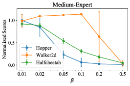
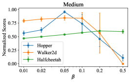
The policy model is a 2-layer MLP with 256 hidden units and ReLU activations. It is trained for 1.0M gradient steps using Adam optimizer with a learning rate of 3e-4 and a batchsize of 256. For all tasks $\omega(t)=\sigma_{t}^{2}$. For the temperature coefficient, we sweep over $\beta\in\{0.01,0.02,0.05,0.1,0.2,0.5\}$ and observe large variances in appropriate values across different tasks (Figure 10). We speculate this might be due to $\beta$ being closely intertwined with the behavior distribution and the variance of the Q-value. These factors might exhibit entirely different characteristics across diverse tasks. Our choices for $\beta$ are detailed in Table 2.

Figure 8: The training instability issue.

Figure 9: Ablation for Antmaze tasks.

Policy extraction (Antmaze).

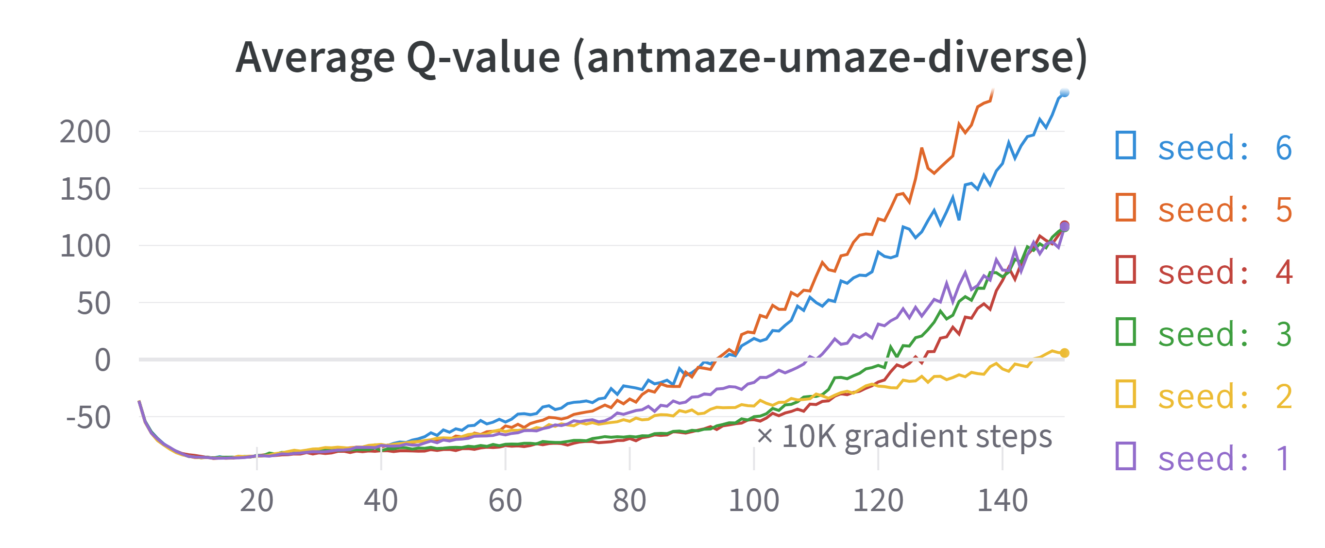
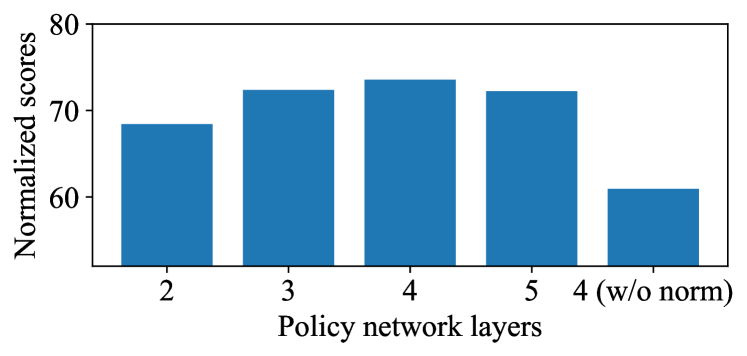
We empirically find that a deeper policy network improves overall performance in Antmaze tasks (Figure 9). As a result, we employ a 4-layer MLP as the policy model. Additionally, we observe that the adopted implicit Q-learning method sometimes has a training instability issue in Antmaze tasks, resulting in highly divergent estimated Q-values (Figure 9). To stabilize training for policy extraction, we replace the temperature coefficient $\beta$ with $\beta_{\text{norm}}({\bm{s}},{\bm{a}}):=\frac{\beta}{\|\nabla_{\bm{a}}Q({\bm{s}},{\bm{a}})\|_{2}}$. We sweep over $\beta\in\{0.01,0.02,...,0.05\}$ for umaze environments, and $\beta\in\{0.03,0.04,...,0.08\}$ for other environments. Our choices for $\beta$ are detailed in Table 2. Other hyperparameters remain consistent with those in the locomotion tasks.

Evaluation.

We run all experiments over 6 independent trials. For each trial, we additionally collect the evaluation score averaged across 20 test episodes at regular intervals for plots in Figure 11. The average performance at the end of training is reported in Table 1. We use NVIDIA A40 GPUs for reporting computing results in Figure 1.

Figure 10: Ablation of the temperature coefficient $\beta$ in D4RL benchmarks.

Locomotion-Medium-Expert	Walker2d	Halfcheetah	Hopper
	0.1	0.01	0.01
Locomotion-Medium	Walker2d	Halfcheetah	Hopper
	0.05	0.2	0.05
Locomotion-Medium-Replay	Walker2d	Halfcheetah	Hopper
	0.5	0.2	0.2
AntMaze-Fixed	Umaze	Medium	Large
	0.02	0.08	0.06
AntMaze-Diverse	Umaze	Medium	Large
	0.04	0.05	0.05

Table 2: Temperature coefficient $\beta$ for every individual task.

Appendix D Training Curves for Offline Reinforcement Learning

Figure 11: Training curves of SRPO (ours) and several baselines. Scores are normalized according to Fu et al. (2020).

References

- Ajay et al. (2023) Anurag Ajay, Yilun Du, Abhi Gupta, Joshua B. Tenenbaum, Tommi S. Jaakkola, and Pulkit Agrawal. Is conditional generative modeling all you need for decision making? In The Eleventh International Conference on Learning Representations, 2023.
- Bishop & Nasrabadi (2006) Christopher M Bishop and Nasser M Nasrabadi. Pattern recognition and machine learning, volume 4. Springer, 2006.
- Chen et al. (2023) Huayu Chen, Cheng Lu, Chengyang Ying, Hang Su, and Jun Zhu. Offline reinforcement learning via high-fidelity generative behavior modeling. In The Eleventh International Conference on Learning Representations, 2023.
- Dhariwal & Nichol (2021) Prafulla Dhariwal and Alexander Quinn Nichol. Diffusion models beat GANs on image synthesis. In Advances in Neural Information Processing Systems, 2021.
- Fu et al. (2020) Justin Fu, Aviral Kumar, Ofir Nachum, George Tucker, and Sergey Levine. D4rl: Datasets for deep data-driven reinforcement learning. arXiv preprint arXiv:2004.07219, 2020.
- Fujimoto & Gu (2021) Scott Fujimoto and Shixiang Shane Gu. A minimalist approach to offline reinforcement learning. Advances in neural information processing systems, 34:20132–20145, 2021.
- Fujimoto et al. (2019) Scott Fujimoto, David Meger, and Doina Precup. Off-policy deep reinforcement learning without exploration. In Proceedings of the 36th International Conference on Machine Learning, 2019.
- Goo & Niekum (2022) Wonjoon Goo and Scott Niekum. Know your boundaries: The necessity of explicit behavioral cloning in offline rl. arXiv preprint arXiv:2206.00695, 2022.
- Gretton et al. (2007) Arthur Gretton, Karsten M Borgwardt, Malte Rasch, Bernhard Schölkopf, and Alexander J Smola. A kernel approach to comparing distributions. In Proceedings of the National Conference on Artificial Intelligence, 2007.
- Hansen-Estruch et al. (2023) Philippe Hansen-Estruch, Ilya Kostrikov, Michael Janner, Jakub Grudzien Kuba, and Sergey Levine. Idql: Implicit q-learning as an actor-critic method with diffusion policies. arXiv preprint arXiv:2304.10573, 2023.
- Ho et al. (2020) Jonathan Ho, Ajay Jain, and Pieter Abbeel. Denoising diffusion probabilistic models. In Advances in Neural Information Processing Systems, 2020.
- Janner et al. (2022) Michael Janner, Yilun Du, Joshua Tenenbaum, and Sergey Levine. Planning with diffusion for flexible behavior synthesis. In International Conference on Machine Learning, 2022.
- Kang et al. (2023) Bingyi Kang, Xiao Ma, Chao Du, Tianyu Pang, and Shuicheng Yan. Efficient diffusion policies for offline reinforcement learning. arXiv preprint arXiv:2305.20081, 2023.
- Kingma & Welling (2014) Diederik P. Kingma and Max Welling. Auto-encoding variational bayes. In 2nd International Conference on Learning Representations, 2014.
- Kostrikov et al. (2021) Ilya Kostrikov, Rob Fergus, Jonathan Tompson, and Ofir Nachum. Offline reinforcement learning with fisher divergence critic regularization. In International Conference on Machine Learning, pp. 5774–5783. PMLR, 2021.
- Kostrikov et al. (2022) Ilya Kostrikov, Ashvin Nair, and Sergey Levine. Offline reinforcement learning with implicit Q-learning. In International Conference on Learning Representations, 2022.
- Kumar et al. (2019) Aviral Kumar, Justin Fu, Matthew Soh, George Tucker, and Sergey Levine. Stabilizing off-policy q-learning via bootstrapping error reduction. Advances in Neural Information Processing Systems, 2019.
- Lu et al. (2022) Cheng Lu, Yuhao Zhou, Fan Bao, Jianfei Chen, Chongxuan Li, and Jun Zhu. Dpm-solver: A fast ode solver for diffusion probabilistic model sampling in around 10 steps. arXiv preprint arXiv:2206.00927, 2022.
- Lu et al. (2023) Cheng Lu, Huayu Chen, Jianfei Chen, Hang Su, Chongxuan Li, and Jun Zhu. Contrastive energy prediction for exact energy-guided diffusion sampling in offline reinforcement learning. In Proceedings of the 40th International Conference on Machine Learning, 2023.
- Mildenhall et al. (2021) Ben Mildenhall, Pratul P Srinivasan, Matthew Tancik, Jonathan T Barron, Ravi Ramamoorthi, and Ren Ng. Nerf: Representing scenes as neural radiance fields for view synthesis. Communications of the ACM, 65(1):99–106, 2021.
- Pearce et al. (2022) Tim Pearce, Tabish Rashid, Anssi Kanervisto, David Bignell, Mingfei Sun, Raluca Georgescu, Sergio Valcarcel Macua, Shan Zheng Tan, Ida Momennejad, Katja Hofmann, et al. Imitating human behaviour with diffusion models. In Deep Reinforcement Learning Workshop NeurIPS, 2022.
- Peng et al. (2019) Xue Bin Peng, Aviral Kumar, Grace Zhang, and Sergey Levine. Advantage-weighted regression: Simple and scalable off-policy reinforcement learning. arXiv preprint arXiv:1910.00177, 2019.
- Peters et al. (2010) Jan Peters, Katharina Mulling, and Yasemin Altun. Relative entropy policy search. In Twenty-Fourth AAAI Conference on Artificial Intelligence, 2010.
- Poole et al. (2023) Ben Poole, Ajay Jain, Jonathan T. Barron, and Ben Mildenhall. Dreamfusion: Text-to-3d using 2d diffusion. In The Eleventh International Conference on Learning Representations, 2023.
- Roeder et al. (2017) Geoffrey Roeder, Yuhuai Wu, and David K Duvenaud. Sticking the landing: Simple, lower-variance gradient estimators for variational inference. Advances in Neural Information Processing Systems, 30, 2017.
- Saharia et al. (2022) Chitwan Saharia, William Chan, Saurabh Saxena, Lala Li, Jay Whang, Emily L Denton, Kamyar Ghasemipour, Raphael Gontijo Lopes, Burcu Karagol Ayan, Tim Salimans, et al. Photorealistic text-to-image diffusion models with deep language understanding. Advances in Neural Information Processing Systems, 35:36479–36494, 2022.
- Sohl-Dickstein et al. (2015) Jascha Sohl-Dickstein, Eric Weiss, Niru Maheswaranathan, and Surya Ganguli. Deep unsupervised learning using nonequilibrium thermodynamics. In International Conference on Machine Learning, pp. 2256–2265, 2015.
- Song et al. (2021) Yang Song, Jascha Sohl-Dickstein, Diederik P Kingma, Abhishek Kumar, Stefano Ermon, and Ben Poole. Score-based generative modeling through stochastic differential equations. In International Conference on Learning Representations, 2021.
- Sutton & Barto (1998) Richard S. Sutton and Andrew G. Barto. Introduction to Reinforcement Learning. MIT Press, Cambridge, MA, USA, 1st edition, 1998. ISBN 0262193981.
- Wang et al. (2023a) Zhendong Wang, Jonathan J Hunt, and Mingyuan Zhou. Diffusion policies as an expressive policy class for offline reinforcement learning. In The Eleventh International Conference on Learning Representations, 2023a.
- Wang et al. (2023b) Zhengyi Wang, Cheng Lu, Yikai Wang, Fan Bao, Chongxuan Li, Hang Su, and Jun Zhu. Prolificdreamer: High-fidelity and diverse text-to-3d generation with variational score distillation. arXiv preprint arXiv:2305.16213, 2023b.
- Wu et al. (2022) Jialong Wu, Haixu Wu, Zihan Qiu, Jianmin Wang, and Mingsheng Long. Supported policy optimization for offline reinforcement learning. Advances in Neural Information Processing Systems, 2022.
- Wu et al. (2019) Yifan Wu, George Tucker, and Ofir Nachum. Behavior regularized offline reinforcement learning. arXiv preprint arXiv:1911.11361, 2019.
- Xu et al. (2021) Haoran Xu, Xianyuan Zhan, Jianxiong Li, and Honglei Yin. Offline reinforcement learning with soft behavior regularization. arXiv preprint arXiv:2110.07395, 2021.
- Xu et al. (2022) Minkai Xu, Lantao Yu, Yang Song, Chence Shi, Stefano Ermon, and Jian Tang. Geodiff: A geometric diffusion model for molecular conformation generation. In International Conference on Learning Representations, 2022.
- Yue et al. (2022) Yang Yue, Bingyi Kang, Xiao Ma, Zhongwen Xu, Gao Huang, and Shuicheng Yan. Boosting offline reinforcement learning via data rebalancing. arXiv preprint arXiv:2210.09241, 2022.