The Allen-Cahn equation with nonlinear truncated Laplacians: description of radial solutions

Abstract

We consider the Allen-Cahn equation with the so-called truncated Laplacians, which are fully nonlinear differential operators that depend on some eigenvalues of the Hessian matrix. By monitoring the sign of a quantity that is responsible for switches from a first order ODE regime to a second order ODE regime (and vice versa), we give a nearly complete description of radial solutions. In particular, we reveal the existence of surprising unbounded radial solutions. Also radial solutions cannot oscillate, which is in sharp contrast with the case of the Laplacian operator, or that of Pucci’s operators.

Key Words: fully nonlinear differential operator, Allen-Cahn nonlinearity, radial solutions, switches.

AMS Subject Classifications: 35J70, 34C26, 34C25, 35B30.

Matthieu Alfaro and Philippe Jouan

1 Introduction

This work is concerned with the highly degenerate partial differential equations

$$\mathcal{P}_{k}^{-}U+g(U)=0\quad\text{ in }\mathbb{R}^{N},$$ (1)

and

$$\mathcal{P}_{k}^{+}U+g(U)=0\quad\text{ in }\mathbb{R}^{N}.$$ (2)

Here $N\geq 2$ and, for $1\leq k<N$, $\mathcal{P}_{k}^{-}$ et $\mathcal{P}_{k}^{+}$ denote the so-called nonlinear truncated Laplacian operators. The nonlinearity $g$ is of the bistable type, a typical example being the Allen-Cahn nonlinearity $g(U)=U-U^{3}$. In this framework, we give a nearly complete description of radial solutions, revealing sharp differences with the case of the Laplacian operator, or that of Pucci’s operators.

The nonlinear truncated Laplacians are defined as follows. Let $N\geq 2$ be given. For $U:\mathbb{R}^{N}\to\mathbb{R}$, say of the class $\mathcal{C}^{2}$, we denote by

$$\lambda_{1}(D^{2}U)\leq\cdots\leq\lambda_{N}(D^{2}U)$$

the eigenvalues of the Hessian matrix $D^{2}U$. For $1\leq k<N$ we consider the fully nonlinear differential operators given by

$$\mathcal{P}_{k}^{-}U:=\sum_{i=1}^{k}\lambda_{i}(D^{2}U),$$ (3)

and

$$\mathcal{P}_{k}^{+}U:=\sum_{i=N-k+1}^{N}\lambda_{i}(D^{2}U).$$ (4)

These highly degenerate operators have been introduced in the context of differential geometry, by Wu [25] and Sha [24], in order to solve problems related to manifolds with partial positive curvature. They also appear in the analysis of mean curvature flow in arbitrary codimension performed by Ambrosio and Soner [2].

In a PDE context, they are considered as an example of degenerate fully non linear operators in the seminal User’s guide [11], but more recently both Harvey and Lawson in [18, 19] and Caffarelli, Li and Nirenberg [10] have studied them in a completely new light.

In the very last years, some new results have been obtained on Dirichlet problems in bounded domains in relationship with the convexity of the domain, through the study of the maximum principle and the principal eigenvalue, see [22] and [4, 5].

As far as problems in $\mathbb{R}^{N}$ are concerned, we refer to the works of Birindelli, Galise and Leoni [6] and Galise [13] on the existence of steady states (nonlinear Liouville theorems), and to the work [1] on solutions to evolution equations (Heat equations and Fujita blow up phenomena).

Let us also mention the works [8], [7] involving the degenerate operators defined by $\mathcal{P}_{j}U:=\lambda_{j}(D^{2}U)$ for some $1\leq j\leq N$, studying well-posedness of such problems, and their approximation by a two-player zero-sum game.

When considering the Laplacian operator, the search of radial solutions $U(x)=u(|x|)$ to

$$\Delta U+g(U)=0\quad\text{ in }\mathbb{R}^{N},$$

reduces to understanding, for any $\xi\in\mathbb{R}$, the non autonomous second order ODE Cauchy problem

$$u^{\prime\prime}+\frac{N-1}{r}u^{\prime}+g(u)=0\quad\text{ in }(0,+\infty),\quad u(0)=\xi,\quad u^{\prime}(0)=0,$$

where $u=u(r)$. Building on this, one can prove, when $g$ is an odd and bistable nonlinearity, the existence of oscillating solutions which, moreover, are periodic when $N=1$ and localized when $N\geq 2$ (see below for precise definitions). We refer to [21] for such constructions, see also [14] and [15] for related results. Such oscillating radial solutions were also constructed for the bistable prescribed mean curvature equations [23], namely

$$\textrm{div}\left(\frac{\nabla U}{\sqrt{1\pm|\nabla U|^{2}}}\right)+g(U)=0\quad\text{ in }\mathbb{R}^{N},$$

the sign “$+$” corresponding to the Euclidian case, the sign “$-$” to the Lorentz-Minkowski case.

Very recently, the case of Pucci’s extremal operators was studied by d’Avenia and Pomponio [12]. In contrast with the Laplacian operator or the mean curvature operator, the Pucci’s operators of radial functions may take two different forms depending on the sign of $u^{\prime\prime}(r)$. Because of that, in order to construct radial solutions, one needs to monitor the quantity $u^{\prime\prime}(r)$ and may have to glue solutions of two different second order ODE Cauchy problems. Nevertheless, as proved in [12], oscillating radial solutions still exist.

The nonlinear truncated Laplacian operators share with Pucci’s operators the property of switching their expressions depending on the sign of a quantity, namely $u^{\prime\prime}(r)-\frac{1}{r}u^{\prime}(r)$. Tracking such a quantity is far from trivial and, moreover, when a switch occurs, one has to glue a solution of a first order ODE with a solution of a second order ODE. This makes the analysis rather involved and outcomes are in sharp contrast with the aforementioned equations. In particular, it turns out that equations (1) and (2) support the existence of unexpected unbounded solutions but, on the other hand, do not admit any oscillating (radial) solutions.

2 Main results

We consider a bistable nonlinearity $g$, a typical example being the Allen-Cahn nonlinearity $g(U)=U-U^{3}$. More generally, we always assume the following.

Assumption 2.1 (Bistable nonlinearity).

The nonlinearity $g:\mathbb{R}\to\mathbb{R}$ is odd, and of the class $\mathcal{C}^{1}$ on $\mathbb{R}$. There are $0<\beta<\alpha$ such that

1. $g>0$ on $(0,\alpha)$, $g<0$ on $(\alpha,+\infty)$,

2. $g^{\prime}>0$ on $[0,\beta)$, $g^{\prime}<0$ on $(\beta,+\infty)$,

3. $g$ is twice differentiable at $\pm\beta$ and $g^{\prime\prime}(\beta)<0$.

In this work, by (radial) solution to (1), or (2), we always mean the following.

Definition 2.2 (Radial solutions).

A radial solution to (1), or (2), is a $0<R\leq+\infty$ and a piecewise $\mathcal{C}^{2}$ function $u:[0,R)\to\mathbb{R}$, with $u^{\prime}(0)=0$, such that $U(x):=u(|x|)$ solves (1), or (2), on $B(0,R)$. Also if $R<+\infty$ we require $|u(r)|+|u^{\prime}(r)|\to+\infty$ as $r\nearrow R$, meaning that the solution is maximal.

It is said oscillating if $R=+\infty$ and $u$, nontrivial, has an unbounded sequence of zeros.

It is said localized if $R=+\infty$ and $u(+\infty)=0$.

Remark 2.3 (Regularity of radial solutions).

Following the construction in Section 4, one can easily see that some solutions $u$ are of the class $\mathcal{C}^{2}$ on $[0,R)$, while some are only of the class $\mathcal{C}^{1}$ on $[0,R)$, $\mathcal{C}^{2}$ on $[0,R)\setminus\{t_{2\rightarrow 1}\}$ for some switching point $t_{2\rightarrow 1}$, with $u^{\prime\prime}(t_{2\rightarrow 1}^{-})>u^{\prime\prime}(t_{2\rightarrow 1}^{+})$. This jump in the second derivative occurs when the operator switches from a second order regime to a first order regime (the other way being harmless). See below for details.

Remark 2.4 (Considering (2) is enough).

Since $\mathcal{P}_{k}^{-}U=-\mathcal{P}_{k}^{+}(-U)$ and $g$ is odd, we deduce that $U$ solves (1) if and only if $-U$ solves (2). As a result, we focus only on equation (2), but any of our stated result has its immediate counterpart for equation (1).

In order to state our main results, we need to define the following critical value: from Assumption 2.1 there is a unique $\xi^{*}=\xi^{*}(k)\in(\beta,\alpha)$ such that

$$kg^{2}(\beta)\int_{\beta}^{\xi^{*}}\frac{ds}{g(s)}=\int_{\beta}^{\alpha}g(s)ds.$$ (5)

We now state our main result for $k=1$, a case for which our description of radial solutions is exhaustive.

Theorem 2.5 (Radial solutions, $k=1$).

Let $k=1$. Then for any $\xi\in\mathbb{R}$, there is a unique radial solution to (2) starting from $u(0)=\xi$. Moreover, depending on $\xi$, it has the following properties.

1. If $\xi\in\{-\alpha,0,\alpha\}$ then $u$ is constant (and $R=+\infty$).

2. If $\xi<-\alpha$ then $u^{\prime}<0$ on $(0,R)$, $u(r)\to-\infty$ as $r\nearrow R$.

3. If $\xi>\alpha$ then $u^{\prime}>0$ on $(0,R)$, $u(r)\to+\infty$ as $r\nearrow R$.

4. If $-\alpha<\xi<0$ then $R=+\infty$, $u^{\prime}>0$ on $(0,+\infty)$, and $u(+\infty)=0$.

5. If $0<\xi<\alpha$ then the three following outcomes are possible.

   1. If $\xi^{*}<\xi<\alpha$ then $u^{\prime}<0$ on $(0,R)$, $u(r)\to-\infty$ as $r\nearrow R$.

   2. If $\xi=\xi^{*}$ then $R=+\infty$, $u^{\prime}<0$ on $(0,+\infty)$, $u(+\infty)=-\alpha$.

   3. If $0<\xi<\xi^{*}$ then $R=+\infty$, there is $b>0$ such that $u^{\prime}<0$ on $(0,b)$, $u(b)<0$, $u^{\prime}>0$ on $(b,+\infty)$, and $u(+\infty)=0$.

Hence depending on the initial value $\xi$, radial solutions can be: $(i)$ constant; $(ii)$ negative, decreasing and unbounded; $(iii)$ positive, increasing and unbounded; $(iv)$ negative, increasing and localized; $(v)$-$(a)$ sign changing, decreasing and unbounded; $(v)$-$(b)$ sign-changing, decreasing and bounded; $(v)$-$(c)$ sign-changing, decreasing-increasing and localized. Note that, when $k=1$, equations (1) and (2) do not admit periodic solutions, which is in sharp contrast with the case of the Laplacian [21] and of the Pucci’s operators [12].

As revealed below in (10), if $u^{\prime\prime}(r)-\frac{1}{r}u^{\prime}(r)\geq 0$ then $\mathcal{P}_{1}^{+}U(x)=u^{\prime\prime}(r)$, corresponding to the Laplacian in dimension $k=1$. Nevertheless, for $|\xi|<\alpha$, the behaviour of radial solutions to (2) is very different from those to the bistable equation involving the Laplacian operator in dimension one, namely

$$v^{\prime\prime}+g(v)=0,\quad v(0)=\xi\in(-\alpha,\alpha),\quad v^{\prime}(0)=0,$$ (6)

which are all bounded, in sharp contrast with the case $(v)$-$(a)$ of Theorem 2.5, sign-changing, in sharp contrast with the case $(iv)$ of Theorem 2.5, and periodic, in sharp contrast with the cases $(iv)$ and $(v)$ of Theorem 2.5. The reason is that, as revealed below in (10), if $u^{\prime\prime}(r)-\frac{1}{r}u^{\prime}(r)\leq 0$ then $\mathcal{P}_{1}^{+}U(x)=\frac{1}{r}u^{\prime}(r)$. As a result, before entering the “Laplacian in dimension one regime”, the energy of the solution may be increased by a “first order ODE regime”, explaining $(v)$-$(a)$ and $(v)$-$(b)$. Also, the solution always finishes his way by the “first order ODE regime”, which prevents oscillations that one may have expected, for instance in the case $(v)$-$(c)$.

We now state our main result for $k\geq 2$.

Theorem 2.6 (Radial solutions, $k\geq 2$).

Let $k\geq 2$. Then for any $\xi\in\mathbb{R}$, there is a unique radial solution to (2) starting from $u(0)=\xi$. Moreover, depending on $\xi$, it has the following properties.

1. If $\xi\in\{-\alpha,0,\alpha\}$ then $u$ is constant (and $R=+\infty$).

2. If $\xi<-\alpha$ then $u^{\prime}<0$ on $(0,R)$, $u(r)\to-\infty$ as $r\nearrow R$.

3. If $\xi>\alpha$ then $u^{\prime}>0$ on $(0,R)$, $u(r)\to+\infty$ as $r\nearrow R$.

4. If $-\alpha<\xi<0$ then $R=+\infty$, $u^{\prime}>0$ on $(0,+\infty)$, and $u(+\infty)=0$.

5. If $0<\xi<\alpha$ then there are positive numbers $\underline{\xi}$, $\xi^{**}$, $\overline{\xi}$ satisfying $\beta<\underline{\xi}\leq\xi^{**}\leq\overline{\xi}<\alpha$ such that the three following outcomes are possible.

   1. If $\overline{\xi}<\xi<\alpha$ then $u^{\prime}<0$ on $(0,R)$, $u(r)\to-\infty$ as $r\nearrow R$.

   2. If $\xi=\xi^{**}$ then $R=+\infty$, $u^{\prime}<0$ on $(0,+\infty)$, $u(+\infty)=-\alpha$.

   3. If $0<\xi<\underline{\xi}$ then $R=+\infty$, there is $b>0$ such that $u^{\prime}<0$ on $(0,b)$, $u(b)<0$, $u^{\prime}>0$ on $(b,+\infty)$, and $u(+\infty)=0$.

We conjecture that, in the setting of Theorem 2.6, we may take $\underline{\xi}=\xi^{**}=\overline{\xi}$, so that the above description would be exhaustive. We refer to Theorem 3.8 and Remark 3.9 for further details and comments on this delicate issue.

Let us underline that, using the one-to-one relation (38) (see also subsection 4.2.2) and the lower bound in (25), one can check that $\underline{\xi}>\xi^{*}$, where $\xi^{*}=\xi^{*}(k)$ is defined through (5). Roughly speaking, this means that there are “more” localized solutions, of the type $(v)$-$(c)$, in the $k\geq 2$ case than in the $k=1$ case. The reason is the following. As revealed below in (10), if $u^{\prime\prime}(r)-\frac{1}{r}u^{\prime}(r)\geq 0$ then $\mathcal{P}_{k}^{+}U(x)=u^{\prime\prime}(r)+\frac{k-1}{r}u^{\prime}(r)$, corresponding to the Laplacian in dimension $k$. In this regime, we therefore have to deal with a non autonomous second order ODE when $k\geq 2$, which typically dampens oscillations. Consequently, the possible increase of the energy through a “first order regime” — when $u^{\prime\prime}(r)-\frac{1}{r}u^{\prime}(r)\leq 0$— is less sensitive when $k\geq 2$.

Note that, when $k\geq 2$, equations (1) and (2) do not admit oscillating solutions, which is again in sharp contrast with the case of the Laplacian [21] and of the Pucci’s operators [12].

The organization of the paper is as follows. Some preliminaries are presented in Section 3: identification of two distinct regimes for the computation of the nonlinear truncated Laplacians of radial functions, and analysis of the needed ODE Cauchy problems. In Section 4, we prove Theorem 2.5 and Theorem 2.6, thus giving a complete description of radial solutions when $k=1$, and a nearly complete one when $k\geq 2$.

3 Preliminaries

3.1 Truncated Laplacians of radial functions

Consider a radial function

$$U(x):=u\left(|x|\right),$$ (7)

for some $u=u(r)$, and where $|x|=(x_{1}^{2}+\cdots+x_{N}^{2})^{1/2}$. We also require $u^{\prime}(0)=0$.

After straightforward computations, we obtain the Hessian matrix

$$D^{2}U(x)=\frac{1}{|x|}u^{\prime}(r)Id_{N}-\left(\frac{1}{|x|}u^{\prime}(r)-u^{\prime\prime}(r)\right)\frac{x}{|x|}\otimes\frac{x}{|x|},\quad\text{ for all }x\neq 0,$$

where we understand $|x|=r$. Since $\frac{x}{|x|}\otimes\frac{x}{|x|}$ is a matrix of rank 1, $\frac{1}{|x|}u^{\prime}(r)$ is an eigenvalue of $D^{2}U(x)$ with multiplicity (at least) $N-1$. By considering the trace of the Hessian matrix we see that the remaining eigenvalue has to be $u^{\prime\prime}(r)$. As a result, comparing $\frac{1}{|x|}u^{\prime}(r)$ and $u^{\prime\prime}(r)$ is enough to compute $\mathcal{P}^{\pm}_{k}U(x)$. More precisely, denoting

$$\mathcal{A}u(r):=u^{\prime\prime}(r)-\frac{1}{r}u^{\prime}(r),$$ (8)

we have

$$\mathcal{P}^{-}_{k}U(x)=\begin{cases}\frac{k}{r}u^{\prime}(r)&\text{ if }\mathcal{A}u(r)\geq 0\vspace{5pt}\\ u^{\prime\prime}(r)+\frac{k-1}{r}u^{\prime}(r)&\text{ if }\mathcal{A}u(r)\leq 0,\end{cases}$$ (9)

whereas

$$\mathcal{P}^{+}_{k}U(x)=\begin{cases}u^{\prime\prime}(r)+\frac{k-1}{r}u^{\prime}(r)&\text{ if }\mathcal{A}u(r)\geq 0\vspace{5pt}\\ \frac{k}{r}u^{\prime}(r)&\text{ if }\mathcal{A}u(r)\leq 0.\end{cases}$$ (10)

As a result, when looking after radial solutions to (1) or (2), we have to deal either with a first order ODE, namely

$$\frac{k}{r}u^{\prime}+g(u)=0,$$

or a second order ODE, namely

$$u^{\prime\prime}+\frac{k-1}{r}u^{\prime}+g(u)=0,$$

depending on the sign of $\mathcal{A}u$, and switches from a regime to another may occur.

3.2 Some first order ODE tools

For $r_{0}\geq 0$ and $\xi\in\mathbb{R}$, we consider the nonlinear first order ODE Cauchy problem

$$\left\{\begin{array}[]{lllll}\varphi^{\prime}&=&-\frac{r}{k}g(\varphi),\\ \varphi(r_{0})&=&\xi,\end{array}\right.$$ (11)

and denote $\varphi(r)=\varphi(r;r_{0},\xi)$ its maximal solution defined on some open interval $I$ containing $r_{0}$.

Lemma 3.1 (First order ODE Cauchy problem).

If $|\xi|\leq\alpha$ then the solution $\varphi$ is global. Next, depending on the initial data $\xi$, the following holds.

1. If $\xi\in\{-\alpha,0,+\alpha\}$ then $\varphi$ is constant.

2. If $0<\xi<+\alpha$ then $\varphi^{\prime}<0$ on $(r_{0},+\infty)$, and $\varphi(r)\to 0$ as $r\to+\infty$.

   If $-\alpha<\xi<0$ then $\varphi^{\prime}>0$ on $(r_{0},+\infty)$, and $\varphi(r)\to 0$ as $r\to+\infty$.

3. If $\xi>+\alpha$ then $\varphi^{\prime}>0$ on $I\cap(r_{0},+\infty)$, and $\varphi(r)\to+\infty$ as $r\to\sup I$.

   If $\xi<-\alpha$ then $\varphi^{\prime}<0$ on $I\cap(r_{0},+\infty)$, and $\varphi(r)\to-\infty$ as $r\to\sup I$.

Last, in any case, we have

$$\mathcal{A}\varphi(r) = -\frac{r}{k}\varphi^{\prime}(r)g^{\prime}(\varphi(r))=\frac{r^{2}}{k^{2}}g(\varphi(r))g^{\prime}(\varphi(r)),\quad\forall r\in I,$$ (12)

$$(\mathcal{A}\varphi)^{\prime}(r) = \left(\frac{2}{r}-\frac{r}{k}g^{\prime}(\varphi(r))\right)\mathcal{A}\varphi(r)-\frac{r}{k}{\varphi^{\prime}}^{2}(r)g^{\prime\prime}(\varphi(r)),\quad\forall r\in I\setminus\{0\},$$ (13)

the latter obviously holding true when $g$ is twice differentiable at $\varphi(r)$ (in particular when $\varphi(r)=\pm\beta$).

Proof.

Item $(i)$ is clear since $-\alpha$, $0$ and $\alpha$ are the three zeros of $g$.

Let us prove $(ii)$. Assume $0<\xi<\alpha$, the other case being similar. Then, from Cauchy-Lipschitz theorem, $\varphi(r)$ is trapped in $(0,\alpha)$ so that not only $I=\mathbb{R}$, but also $\varphi^{\prime}<0$ on $(r_{0},+\infty)$ from the ODE and Assumption 2.1. Denote

$$H(t):=\int_{t}^{\xi}\frac{ds}{g(s)},\quad 0<t\leq\xi.$$ (14)

From Assumption 2.1, $H$ is a decreasing bijection from $(0,\xi)$ to $(0,+\infty)$. By separating variables, we can compute

$$\varphi(r)=H^{-1}\left(\frac{r^{2}-r_{0}^{2}}{2k}\right)\to 0,\quad\text{ as }r\to+\infty.$$ (15)

Let us prove $(iii)$. Assume $\xi>\alpha$, the other case being similar. Then, from Cauchy-Lipschitz theorem, $\varphi(r)$ is trapped in $(\alpha,+\infty)$ so that $\varphi^{\prime}>0$ on $I\cap(r_{0},+\infty)$ from the ODE and Assumption 2.1. If $\sup I<+\infty$ then one must have $\varphi(r)\to+\infty$ as $r\to\sup I$. On the other hand, if $\sup I=+\infty$ then, from the ODE, the limit in $+\infty$ cannot be finite (otherwise $\varphi^{\prime}(r)\to+\infty$ which is a contradiction), and thus has to be $+\infty$.

Last, recalling $\mathcal{A}\varphi(r)=\varphi^{\prime\prime}(r)-\frac{1}{r}\varphi^{\prime}(r)$, we differentiate once the ODE (11) to reach (12), that we differentiate to get (13). ∎

For a solution $\varphi$, we say that $\mathcal{A}\varphi$ ceases to be nonpositive at $s_{0}>0$ if $(i)$ there is ${\varepsilon}_{1}>0$ such that $\mathcal{A}\varphi\leq 0$ on $(s_{0}-{\varepsilon}_{1},s_{0})$ and $(ii)$ for all ${\varepsilon}_{2}>0$, there is $s^{*}\in(s_{0},s_{0}+{\varepsilon}_{2})$ such that $\mathcal{A}\varphi(s^{*})>0$.

Corollary 3.2.

$\mathcal{A}\varphi$ ceases to be nonpositive at $s_{0}>0$ if and only if $\varphi(s_{0})=\beta$; and, if so, there is ${\varepsilon}_{3}>0$ such that $\mathcal{A}\varphi>0$ on $(s_{0},s_{0}+{\varepsilon}_{3})$.

Proof.

If $\mathcal{A}\varphi$ ceases to be nonpositive at $s_{0}>0$ then $\mathcal{A}\varphi(s_{0})=0$. We deduce from (12) that $g(\varphi(s_{0}))g^{\prime}(\varphi(s_{0}))=0$. If $g(\varphi(s_{0}))=0$ then $\varphi(s_{0})\in\{-\alpha,0,\alpha\}$ and, from the equation for $\varphi$, $\varphi^{\prime}(s_{0})=0$ so that $\varphi$ is constant, which is a contradiction. Hence $g^{\prime}(\varphi(s_{0}))=0$, meaning $\varphi(s_{0})=\pm\beta$, and, from (13) and the equation for $\varphi$, we have $(\mathcal{A}\varphi)^{\prime}(s_{0})=-\frac{s_{0}^{3}}{k^{3}}g^{2}(\pm\beta)g^{\prime\prime}(\pm\beta)$ which, see Assumption 2.1, is negative at $-\beta$ (hence a contradiction) and positive at $+\beta$. The converse is obviously true since then $\mathcal{A}\varphi(s_{0})=0$ and $(\mathcal{A}\varphi)^{\prime}(s_{0})>0$. ∎

3.3 Some second order ODE tools

For $r_{0}\geq 0$, $\xi\in\mathbb{R}$ and $\theta\in\mathbb{R}$ with

$$(r_{0},\theta)\in(0,+\infty)\times\mathbb{R}\cup\{(0,0)\},$$ (16)

we consider the nonlinear second order ODE Cauchy problem

$$\left\{\begin{array}[]{lllll}\psi^{\prime\prime}+\frac{k-1}{r}\psi^{\prime}+g(\psi)&=&0,\\ \psi(r_{0})&=&\xi,\\ \psi^{\prime}(r_{0})&=&\theta,\end{array}\right.$$ (17)

and denote by $\psi(r)=\psi(r;r_{0},\xi,\theta)$ its maximal solution defined on some open interval $J$ containing $r_{0}$.

Remark 3.3 (Sturm-Liouville approach).

Stricto sensu, when $k\neq 1$ and $(r_{0},\theta)=(0,0)$, the Cauchy-Lipschitz theorem does not apply to (17). However using a Sturm-Liouville approach, one can write $(r^{k-1}\psi^{\prime})^{\prime}=-r^{k-1}g(\psi(r))$ so that

$$\psi^{\prime}(r)=-\frac{1}{r^{k-1}}\int_{0}^{r}s^{k-1}g(\psi(s))ds,$$ (18)

and then recast the ODE problem (17) into the integral equation

$$\psi(r)=\xi-\int_{0}^{r}\frac{1}{s^{k-1}}\int_{0}^{s}t^{k-1}g(\psi(t))dtds.$$

Under this form one can then prove that the conclusion of the Cauchy-Lipschitz theorem does hold, see [17, Proposition 3.1] among others.

Furthermore, when $k\geq 2$, if $\psi$ solves the second order ODE on $(0,R)$ and can be extended by continuity at $r=0$, say $\psi(0)=\xi\in\mathbb{R}$, then, necessarily, $\psi^{\prime}(0)=0$ and $\psi^{\prime\prime}(0)=-\frac{g(\xi)}{k}$ (notice that the solution $\varphi$ to the first order Cauchy problem (11) also obviously satisfies $\varphi^{\prime}(0)=0$ and $\varphi^{\prime\prime}(0)=-\frac{g(\xi)}{k}$). Indeed, the Sturm-Liouville approach provides, for any $0<r_{0}<r<R$,

$$r^{k-1}\psi^{\prime}(r)-r_{0}^{k-1}\psi^{\prime}(r_{0})=-\int_{r_{0}}^{r}s^{k-1}g(\psi(s))ds.$$

The right hand side has a finite limit as $r_{0}\to 0$ and, thus, so has $r_{0}^{k-1}\psi^{\prime}(r_{0})$; since $k\geq 2$ and $\psi(0)=\xi$, this limit has to be zero. As a result (18) is still valid and can be recast

$$\psi^{\prime}(r)=-r\int_{0}^{1}z^{k-1}g(\psi(rz))dz,$$

so that $\psi^{\prime}(0)=0$ and $\frac{\psi^{\prime}(r)}{r}\to-\frac{g(\xi)}{k}$ as $r\to 0$, as announced. In particular, when $k\geq 2$, the requirement $u^{\prime}(0)=0$ is automatically satisfied by solutions in the sense of Definition 2.2 (and also by all solutions that can be extended to zero, see subsection 4.3).

Lemma 3.4 (Monitoring $\mathcal{A}\psi$).

We have, for all $r\in J\setminus\{0\}$,

$$\mathcal{A}\psi(r) = -\frac{k}{r}\psi^{\prime}(r)-g(\psi(r)),$$ (19)

$$(\mathcal{A}\psi)^{\prime}(r) = -\frac{k}{r}\mathcal{A}\psi(r)-\psi^{\prime}(r)g^{\prime}(\psi(r)),$$ (20)

$$(\mathcal{A}\psi)^{\prime\prime}(r) = \frac{k}{r^{2}}\mathcal{A}\psi(r)-\frac{k}{r}(\mathcal{A}\psi)^{\prime}(r)-\psi^{\prime\prime}(r)g^{\prime}(\psi(r))-{\psi^{\prime}}^{2}(r)g^{\prime\prime}(\psi(r)),$$ (21)

the latter obviously holding true when $g$ is twice differentiable at $\psi(r)$ (in particular when $\psi(r)=\pm\beta$). Also, for any $r_{0}\in J$,

$$\mathcal{A}\psi(r)=\mathcal{A}\psi(r_{0})\frac{r_{0}^{k}}{r^{k}}-\int_{r_{0}}^{r}\frac{s^{k}}{r^{k}}\psi^{\prime}(s)g^{\prime}(\psi(s))ds,\quad\forall r\in J\setminus\{0\}.$$ (22)

Proof.

Recalling $\mathcal{A}\psi(r)=\psi^{\prime\prime}(r)-\frac{1}{r}\psi^{\prime}(r)$, the three first properties directly follow from using and differentiating the ODE. Last, solving (20) provides the integral representation. ∎

For a solution $\psi$, we say that $\mathcal{A}\psi$ ceases to be nonnegative at $s_{0}>0$ if $(i)$ there is ${\varepsilon}_{1}>0$ such that $\mathcal{A}\psi\geq 0$ on $(s_{0}-{\varepsilon}_{1},s_{0})$ and $(ii)$ for all ${\varepsilon}_{2}>0$, there is $s^{*}\in(s_{0},s_{0}+{\varepsilon}_{2})$ such that $\mathcal{A}\psi(s^{*})<0$.

Corollary 3.5.

$\mathcal{A}\psi$ ceases to be nonnegative at $s_{0}>0$ if and only if $\psi(s_{0})$ belongs to $(-\infty,-\alpha)\cup(-\beta,0)\cup(\beta,\alpha)$ and $\psi^{\prime}(s_{0})=-\frac{s_{0}}{k}g(\psi(s_{0}))$; and, if so, there is ${\varepsilon}_{3}>0$ such that $\mathcal{A}\psi<0$ on $(s_{0},s_{0}+{\varepsilon}_{3})$.

Proof.

If $\mathcal{A}\psi$ ceases to be nonnegative at $s_{0}>0$ then $\mathcal{A}\psi(s_{0})=0$ and $(\mathcal{A}\psi)^{\prime}(s_{0})\leq 0$. We deduce from (19) and (20) that $g(\psi(s_{0}))g^{\prime}(\psi(s_{0}))\leq 0$, which means $\psi(s_{0})\in(-\infty,-\alpha]\cup[-\beta,0]\cup[\beta,\alpha]$. If $\psi(s_{0})\in\{-\alpha,0,\alpha\}$, we deduce from $\psi^{\prime}(s_{0})=-\frac{s_{0}}{k}g(\psi(s_{0}))=0$ that $\psi$ is constant, which is a contradiction. If $\psi(s_{0})=\pm\beta$, we deduce from (19) and (20) that $\mathcal{A}\psi(s_{0})=(\mathcal{A}\psi)^{\prime}(s_{0})=0$, which enforces $(\mathcal{A}\psi)^{\prime\prime}(s_{0})=0$, which is contradicted by (21). Hence $\psi(s_{0})\in(-\infty,-\alpha)\cup(-\beta,0)\cup(\beta,\alpha)$ and $\psi^{\prime}(s_{0})=-\frac{s_{0}}{k}g(\psi(s_{0}))$. The converse is obviously true since then $\mathcal{A}\psi(s_{0})=0$ and $(\mathcal{A}\psi)^{\prime}(s_{0})<0$. ∎

We now distinguish the case $k=1$ from the case $k\geq 2$.

3.3.1 The autonomous case $k=1$

This case is well understood: apart from being constant, solutions can be unbounded (case $(i)$ below), heteroclinic orbits or standing waves (see $(ii)$ below) or periodic (case $(iii)$ below). In the sequel, we denote

$$G(t):=\int_{0}^{t}g(s)ds.$$

Lemma 3.6 (Second order ODE Cauchy problem, $k=1$).

Let $k=1$. Define the initial energy

$$E=E(\xi,\theta):=\frac{1}{2}\theta^{2}+G(|\xi|).$$ (23)

Depending on the initial data $(\xi,\theta)$, the following holds.

1. If $|\xi|>\alpha$ or $E>G(\alpha)$ then $\psi(r)\to+\infty$ or $\psi(r)\to-\infty$ as $r\to\sup J$.

2. If $|\xi|\leq\alpha$ and $E=G(\alpha)$ the following three situations may occur: if $\theta=0$ then $\psi\equiv-\alpha$ or $\psi\equiv\alpha$; if $\theta<0$ then $\psi^{\prime}<0$ on $\mathbb{R}$, $\psi(-\infty)=\alpha$, $\psi(+\infty)=-\alpha$; if $\theta>0$ then $\psi^{\prime}>0$ on $\mathbb{R}$, $\psi(-\infty)=-\alpha$, $\psi(+\infty)=\alpha$.

3. If $|\xi|<\alpha$ and $0<E<G(\alpha)$ then the solution $\psi$ is trapped in the interval $(-\alpha,\alpha)$, is $T$ periodic for some $T=T(\xi,\theta)>0$, has exactly two zeros on any $[a,a+T)$, has exactly two critical points on any $[a,a+T)$ where it moreover changes monotonicity, is symmetric with respect to any critical point (that is $\psi^{\prime}(r^{*})=0\Rightarrow\psi(r^{*}-\cdot)=\psi(r^{*}+\cdot)$), and is anti-symmetric with respect to any zero (that is $\psi(r^{*})=0\Rightarrow\psi(r^{*}-\cdot)=-\psi(r^{*}+\cdot)$). Moreover $\psi$ is a surjection from $\mathbb{R}$ to $[-M,M]$ where $|\xi|\leq M<\alpha$ is (uniquely) determined by

   $$\int_{|\xi|}^{M}g(s)ds=\frac{1}{2}\theta^{2},$$

   and the period is given by

   $$\frac{T}{2}=\int_{-M}^{M}\frac{ds}{\sqrt{2(E-G(s))}}=2\int_{0}^{M}\frac{ds}{\sqrt{2(E-G(s))}}.$$

4. If $|\xi|\leq\alpha$ and $E=0$, meaning $(\xi,\theta)=(0,0)$, then $\psi\equiv 0$.

Proof.

The associated energy is conserved, that is

$$\frac{1}{2}{\psi^{\prime}}^{2}(r)+G(\psi(r))=E,\quad\forall r\in J.$$ (24)

From this and a standard phase plane analysis, see Figure 1, we classically reach all the desired conclusions. For instance, in the case $(iii)$, it follows from $E<G(\alpha)$ and (24) that $\psi(r)$ cannot touch $\alpha$ nor $-\alpha$. Hence, $\psi(r)$ is trapped in $(-\alpha,\alpha)$, $(\psi(r),\psi^{\prime}(r))$ cannot blow up in finite time, and thus the solution is global. Next, by combining the phase plane analysis and the identity

$$\psi^{\prime}(r)=\pm\sqrt{2(E-G(\psi(r))},$$

we reach the conclusions of $(iii)$. Details are omitted. ∎

Figure 1: Phase plane analysis for (17) with $k=1$ and the cubic nonlinearity $g(\psi)=\frac{1}{4}(\psi-\psi^{3})$. In red, the nullcline $\psi=0$, in green the nullcline $\psi^{\prime}=0$, in blue the trajectory starting from $\xi=0.6$, $\theta=-0.2$, providing a periodic solution.

3.3.2 The non autonomous case $k\geq 2$

The non autonomous case $k\geq 2$ is more tricky. Nevertheless, when $(r_{0},\theta)=(0,0)$, the comprehension of the Cauchy problem is still complete, whatever $k\geq 1$.

Lemma 3.7 (Second order ODE Cauchy problem, the case $(r_{0},\theta)=(0,0)$).

Let $k\geq 1$. Assume $(r_{0},\theta)=(0,0)$. If $|\xi|\leq\alpha$ then the solution $\psi$ is global. Next, depending on the initial data $\xi$, the following holds.

1. If $\xi\in\{-\alpha,0,+\alpha\}$ then $\psi$ is constant.

2. If $0<|\xi|<\alpha$ then $\psi$ is oscillating, satisfies $\|\psi\|_{L^{\infty}(\mathbb{R})}=\xi$,

   $${\psi^{\prime}}^{2}(r)\leq 2\int_{\psi(r)}^{\xi}g(t)dt\leq 2G(\xi),\quad\forall r\in\mathbb{R},$$

   and

   $$\frac{c}{r^{\frac{k-1}{2}}}\leq|\psi(r)|+|\psi^{\prime}(r)|+|\psi^{\prime\prime}(r)|\leq\frac{C}{r^{\frac{k-1}{2}}},\quad\forall r\geq 1,$$

   for some constants $c=c(\xi)>0$, $C=C(\xi)>0$. Moreover, the critical points of $\psi$ on $[0,+\infty)$ form a sequence $0=x_{0}<x_{1}<\cdots<x_{n}\to+\infty$ such that $\psi(x_{k})\psi(x_{k+1})<0$.

3. If $\xi>+\alpha$ then $\psi^{\prime}>0$ on $J\cap(0,+\infty)$, and $\psi(r)\to+\infty$ as $r\to\sup J$.

   If $\xi<-\alpha$ then $\psi^{\prime}<0$ on $J\cap(0,+\infty)$, and $\psi(r)\to-\infty$ as $r\to\sup J$.

Proof.

Item $(i)$ is clear, whereas item $(ii)$ is borrowed from [21], more precisely Proposition 2.3 and Lemma 2.5 together with their proofs.

Let us prove $(iii)$. Since $g$ is odd, we check that $\psi(r;0,-\xi,0)=-\psi(r;0,\xi,0)$, so we only need to consider $\xi>\alpha$. From the ODE we have $\psi^{\prime\prime}(0)=-\frac{g(\xi)}{k}>0$, so that there is ${\varepsilon}>0$ such that $\psi^{\prime}>0$ on $(0,{\varepsilon})$.

Assume by contradiction the existence of $r_{0}>0$ such that $\psi^{\prime}(r_{0})=0$. We may assume that $r_{0}$ is the smallest positive value with this property so that $\psi(r_{0})>\xi>\alpha$ and $\psi^{\prime\prime}(r_{0})\leq 0$. Testing the ODE at $r=r_{0}$ we reach $\psi^{\prime\prime}(r_{0})>0$, a contradiction. As a result $\psi^{\prime}>0$ on $J\cap(0,+\infty)$.

Hence, if $\sup J<+\infty$ then one must have $\psi(r)\to+\infty$ as $r\to\sup J$. On the other hand, if $\sup J=+\infty$, let us assume by contradiction that the limit $\ell>\xi>\alpha$ of $\psi(r)$ in $+\infty$ is finite. From (18) we deduce $\psi^{\prime}(r)\sim\frac{-g(\ell)}{k}r$ as $r\to+\infty$, which contradicts $\ell<+\infty$. As a result, $\ell=+\infty$ and we are done with $(iii)$. ∎

Last, we need a comprehension of the non autonomous case $k\geq 2$, starting from $r_{0}>0$. When $k\geq 2$, oscillations are typically dampened and some solutions, not trapped in the $k=1$ case, become trapped, and thus oscillating, when $k\geq 2$. Note that many results exist [20], [9], [16], when the potential $G$ is convex and/or coercive. In the present bistable situation, the potential $G$ is neither convex nor coercive and, therefore, the issue of blow-up solutions is intricate. Therefore, we believe Theorem 3.8 and its proof are interesting by themselves in the framework of ODEs.

For our purpose in Section 4, we only need to consider the one-parameter family of solutions $\psi(r;r_{0},\xi,\theta)$ with $r_{0}>0$, $\xi=\beta$, $\theta=-\frac{g(\beta)}{k}r_{0}$, which corresponds to a switch from the first order ODE to the second order one for the radial solutions of (2), see Section 4.

Theorem 3.8 (Second order ODE Cauchy problem, the case $r_{0}>0$).

Let $k\geq 2$. For $r_{0}>0$, let us denote $\psi(r):=\psi\left(r;r_{0},\beta,-\frac{g(\beta)}{k}r_{0}\right)$. Then (recall that $G(t)=\int_{0}^{t}g(s)ds$) there are positive real numbers $\underline{r_{0}}$, $r_{0}^{**}$, $\overline{r_{0}}$ satisfying

$$\frac{k\sqrt{2}}{g(\beta)}\left(G(\alpha)-\frac{1}{k}G(\beta)\right)^{\frac{1}{2}}\leq\underline{r_{0}}\leq r_{0}^{**}\leq\overline{r_{0}}\leq\frac{k\sqrt{2}}{g(\beta)}\left(G(\alpha)-G(\beta)+\frac{k-1}{k}g(\beta)(\alpha+\beta)\right)^{\frac{1}{2}},$$ (25)

and such that the following holds.

1. If $0<r_{0}<\underline{r_{0}}$ then, for $r>r_{0}$, the solution $\psi$ is trapped in $(-\alpha,\alpha)$, global, oscillating and localized. Moreover, there is a sequence $r_{0}<r_{1}<\cdots<r_{n}\to+\infty$ such that, for any $k\in\mathbb{N}$, $\psi$ is strictly monotone on $(r_{k},r_{k+1})$, and $\psi(r_{2k})\psi(r_{2k+1})<0$.

2. If $r_{0}=r_{0}^{**}$ then $\psi^{\prime}<0$ on $(r_{0},+\infty)$ and $\psi(+\infty)=-\alpha$.

3. If $r_{0}>\overline{r_{0}}$ then $\psi^{\prime}<0$ on $J\cap(r_{0},+\infty)$, and $\psi(r)\to-\infty$ as $r\to\sup J$.

Remark 3.9 (A conjecture).

As already emphasized above, such an analysis does not stand in the classical frameworks, since the potential $G$ is neither convex nor coercive. Another important difficulty comes from the fact that we look at a one-parameter family: $r_{0}$ determines both the starting point (at $r=r_{0}$) and the starting slope ($\psi^{\prime}(r_{0})=-\frac{g(\beta)}{k}r_{0}$). Because of that, the description in Theorem 3.8 is not exhaustive. In the proof below, we conjecture that the set $B$ is actually a singleton. In other words, we conjecture that, in the setting of Theorem 3.8, we may take $\underline{r_{0}}=r_{0}^{**}=\overline{r_{0}}$.

Proof.

We temporarily denote $\psi(r)=\psi\left(r;r_{0},\beta,-\frac{g(\beta)}{k}r_{0},g\right)$ to remind the dependence on the nonlinearity $g$. We observe that $\psi(r)=v\left(\frac{r}{r_{0}}\right)$, where

$$v(r)=\psi\left(r;1,\beta,-\frac{g(\beta)}{k}r_{0}^{2},r_{0}^{2}g\right).$$

In the sequel, in order to fix the initial point as 1, we work on $v$ and denote $J_{v}$ its maximal interval of validity.

If there is a (first) point $r^{*}>1$ where $v^{\prime}(r^{*})=0$ then, from the equation, $v(r^{*})\in(-\alpha,0)$. Then, using the equation and the energy identity

$$\frac{1}{2}{v^{\prime}}^{2}(r)+r_{0}^{2}G(v(r))=\frac{1}{2}{v^{\prime}}^{2}(t)+r_{0}^{2}G(v(t))-(k-1)\int_{t}^{r}\frac{{v^{\prime}}^{2}(s)}{s}ds,$$ (26)

we easily see that $v$ is trapped in $(-\alpha,\alpha)$, global, oscillating and localized, which corresponds to case $(i)$. On the other hand if $v^{\prime}<0$, note that the situation $v(+\infty)=0$ is excluded by a Sturm separation argument similar to [21, Lemma 2.5]. As a result, we have the partition $(0,+\infty)=A\cup B\cup C$ where

$$A := \{r_{0}>0:\exists r^{*}>1,v^{\prime}(r^{*})=0\text{ and }v(+\infty)=0\}$$

$$B := \{r_{0}>0:v^{\prime}<0\text{ on }[1,+\infty)\text{ and }v(+\infty)=-\alpha\}$$

$$C := \{r_{0}>0:v^{\prime}<0\text{ on }J_{v}\cap[1,+\infty)\text{ and }v(r)\to-\infty\text{ as }r\nearrow\sup J_{v}\}.$$

From the continuity of solutions with respect to initial conditions and parameters, both the sets $A$ and $C$ are open.

Now, returning to $\psi(r)$ we naturally have, see Figure 2,

$$A = \{r_{0}>0:\exists r^{*}>r_{0},\psi^{\prime}(r^{*})=0\text{ and }\psi(+\infty)=0\}$$

$$B = \{r_{0}>0:\psi^{\prime}<0\text{ on }[r_{0},+\infty)\text{ and }\psi(+\infty)=-\alpha\}$$

$$C = \{r_{0}>0:\psi^{\prime}<0\text{ on }J_{\psi}\cap[r_{0},+\infty)\text{ and }\psi(r)\to-\infty\text{ as }r\nearrow\sup J_{\psi}\},$$

with obvious notations.

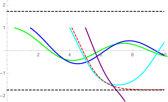
Figure 2: The solutions $\psi\left(r;r_{0},\beta,-\frac{g(\beta)}{k}r_{0}\right)$ with $k=2$, $g(u):=u-\frac{1}{3}u^{3}$ (so that $\beta=1$ and $\alpha=\sqrt{3}$). Solutions of the type $A$: in green $r_{0}=0.5$, in blue $r_{0}=1.5$, in cyan $r_{0}=4$. Solution of the type $B$: in dashed red $r_{0}\approx 4.139$. Solutions of the type $C$: in purple $r_{0}=5$.

Here are a few observations. First, from Lemma 3.4, we have $\mathcal{A}\psi(r_{0})=(\mathcal{A}\psi)^{\prime}(r_{0})=0$ while $(\mathcal{A}\psi)^{\prime\prime}(r_{0})>0$, so that

$$\mathcal{A}\psi>0\text{ on }(r_{0},r_{0}+{\varepsilon}),$$ (27)

for some ${\varepsilon}>0$ (and this is true for any $k\geq 1$). Next, the difference of energy $E(r):=\frac{1}{2}\psi^{\prime 2}(r)+G(\psi(r))$ between points $t$ and $r>t$ is given by

$$E(r)-E(t)=-(k-1)\int_{t}^{r}\frac{\psi^{\prime}(s)}{s}\psi^{\prime}(s)ds.$$ (28)

Notice also that $\frac{d}{dr}\left(\frac{\psi^{\prime}r)}{r}\right)=\frac{1}{r}\mathcal{A}\psi(r)$. It follows that, if we know that $\mathcal{A}\psi\geq 0$ and $\psi^{\prime}<0$ on $(r_{0},r)$, then we have the lower bound

$$E(r)-E(r_{0})\geq-(k-1)\int_{r_{0}}^{r}\frac{\psi^{\prime}(r_{0})}{r_{0}}\psi^{\prime}(s)ds=\frac{k-1}{k}g(\beta)(\psi(r)-\beta).$$ (29)

Building on this, we can pursue and conclude.

$\bullet$ First, if $r_{0}$ is small then the initial energy is small and the damping is large, so that solutions are expected to be trapped and localized. Precisely, let us prove

$$\text{ there is }\;\underline{r_{0}}\geq r_{0}^{loc}:=\frac{k\sqrt{2}}{g(\beta)}\left(G(\alpha)-\frac{1}{k}G(\beta)\right)^{\frac{1}{2}}>0\;\text{ such that }\;(0,\underline{r_{0}})\subset A.$$ (30)

From (27) and Corollary 3.5, we know that $\mathcal{A}\psi\geq 0$ on $(r_{0},r_{1})$ where $r_{1}>r_{0}$ is the first point where $\psi$ values 0. From the equation for $\psi$, we thus have $\frac{\psi^{\prime}(r)}{r}\leq-\frac{1}{k}g(\psi(r))$ on $(r_{0},r_{1})$, so that (28) yields

$$E(r_{1})-E(r_{0})\leq\frac{k-1}{k}\int_{r_{0}}^{r_{1}}g(\psi(s))\psi^{\prime}(s)ds=\frac{k-1}{k}(G(\psi(r_{1}))-G(\beta))=-\frac{k-1}{k}G(\beta).$$ (31)

Now, if $r_{0}\in C$, then $\psi^{\prime}<0$ on $(r_{1},r_{2})$ where $r_{2}>r_{1}$ is the point where $\psi(r_{2})=-\alpha$, and (28) enforces $E(r_{1})\geq E(r_{2})\geq G(-\alpha)=G(\alpha)$. Hence, from (31), $G(\alpha)\leq\frac{1}{2}\frac{g^{2}(\beta)}{k^{2}}r_{0}^{2}+G(\beta)-\frac{k-1}{k}G(\beta)$, that is $r_{0}\geq r_{0}^{loc}$. If $r_{0}\in B$, we find the same estimate $r_{0}\geq r_{0}^{loc}$ (roughly speaking $r_{2}=+\infty$). This proves that $(0,r_{0}^{loc})\subset A$ and thus (30).

$\bullet$ Second, if $r_{0}$ is large then not only the damping is small but also the initial speed is very negative, so that solutions are expected to be non trapped. Precisely, let us prove that

$$\text{ there is }\;\overline{r_{0}}\leq\frac{k\sqrt{2}}{g(\beta)}\left(G(\alpha)-G(\beta)+\frac{k-1}{k}g(\beta)(\alpha+\beta)\right)^{\frac{1}{2}}\;\text{ such that }\;(\overline{r_{0}},+\infty)\subset C.$$ (32)

If $r_{0}\in A$, then there is $r_{1}>r_{0}$ such that $\psi^{\prime}<0$ on $(r_{0},r_{1})$, $\psi^{\prime}(r_{1})=0$, and $\psi(r_{1})\in(-\alpha,0)$; furthermore (27) and Corollary 3.5 enforce $\mathcal{A}\psi\geq 0$ on $(r_{0},r_{1})$. We can thus apply (29) and obtain

$$G(\alpha)-E(r_{0})\geq E(r_{1})-E(r_{0})\geq\frac{k-1}{k}g(\beta)(\psi(r_{1})-\beta)\geq\frac{k-1}{k}g(\beta)(-\alpha-\beta),$$

which means $r_{0}\leq r_{0}^{non-tra}:=\frac{k\sqrt{2}}{g(\beta)}\left(G(\alpha)-G(\beta)+\frac{k-1}{k}g(\beta)(\alpha+\beta)\right)^{\frac{1}{2}}$. If $r_{0}\in B$, we find the same estimate $r_{0}\leq r_{0}^{non-tra}$ (roughly speaking $r_{1}=+\infty$). This proves that $(r_{0}^{non-tra},0)\subset C$ and thus (32).

$\bullet$ Hence, both $A$ and $C$ are open and non empty so that $(0,+\infty)=A\cup B\cup C$ enforces $B$ to be non empty, which completes the proof. ∎

4 Radial solutions

In this section, we will prove Theorem 2.5 ($k=1$) and Theorem 2.6 ($k\geq 2$). Recalling Definition 2.2, we thus look after a $0<R\leq+\infty$ and a piecewise $\mathcal{C}^{2}$ function $u:[0,R)\to\mathbb{R}$, with $u^{\prime}(0)=0$, starting from $u(0)=\xi\in\mathbb{R}$, and such that $U(x):=u(|x|)$ solves (2) on $B(0,R)$. From subsection 3.1, we understood that, depending on the sign of

$$\mathcal{A}u(r):=u^{\prime\prime}(r)-\frac{1}{r}u^{\prime}(r),$$

we are facing either a first order ODE studied in subsection 3.2 or a second order ODE studied in subsection 3.3. We call switching points the points where $\mathcal{A}u(r)$ changes sign, possibly with a jump. If such points exist, in order to construct radial solutions, we need to glue some solutions to (11) with some solutions to (17). It is therefore crucial to determine when a switch occurs at $r_{0}>0$ together with the “starting behaviour” at $r_{0}=0$.

In what follows FOE stands for the First Order Equation (whose solutions are typically denoted $\varphi$) and SOE for the Second Order Equation (whose solutions are typically denoted $\psi$).

Lemma 4.1 (Switching points).

Let $(R,u)$ be a solution to (2) in the sense of Definition 2.2.

1. It switches from FOE to SOE at $r_{0}\in(0,R)$ if and only if $\varphi(r_{0})=\beta$. The solution is then of class $\mathcal{C}^{2}$ in a neighbourhood of $r_{0}$.

2. It switches from SOE to FOE at $r_{0}\in(0,R)$ if and only if $\psi(r_{0})\in(-\infty,-\alpha)\cup(-\beta,0)\cup(\beta,\alpha)$ and $\psi^{\prime}(r_{0})=-\frac{r_{0}}{k}g(\psi(r_{0}))$. The solution is then of class $\mathcal{C}^{1}$ in a neighbourhood of $r_{0}$, but $u^{\prime\prime}(r_{0}^{-})>u^{\prime\prime}(r_{0}^{+})$.

Proof.

Let us prove $(i)$. From Corollary 3.2, the condition $\varphi(r_{0})=\beta$ is necessary for the switch to occur. Conversely, $\varphi(r_{0})=\beta$ enforces $\varphi^{\prime}(r_{0})=-\frac{r_{0}}{k}g(\beta)$ and, $u$ being $\mathcal{C}^{1}$ has to be equal to $\psi=\psi\left(\cdot;r_{0},\beta,-\frac{g(\beta)}{k}r_{0}\right)$, provided by Theorem 3.8, on $(r_{0},r_{1})$ for some $r_{1}>0$. It follows from (27) that the switch has occurred at $r_{0}$. Last, the continuity of $\mathcal{A}u$ implies that of $u^{\prime\prime}$ and the solution $u$ is $\mathcal{C}^{2}$ in a neighbourhood of $r_{0}$.

Let us prove $(ii)$. From Corollary 3.5, the stated conditions are necessary. Conversely, $u$ being $\mathcal{C}^{1}$ has to be equal to $\varphi=\varphi(\cdot;r_{0},\psi(r_{0}))$, defined at the beginning of subsection 3.2, on $(r_{0},r_{1})$ for some $r_{1}>0$. It follows from (12) that $\mathcal{A}\varphi(r_{0})=\frac{r_{0}^{2}}{k^{2}}g(\varphi(r_{0}))g^{\prime}(\varphi(r_{0}))<0$, and thus the switch has occurred at $r_{0}$. Last, $\mathcal{A}\psi(r_{0})=0>\mathcal{A}\varphi(r_{0})$ transfers into $u^{\prime\prime}(r_{0}^{-})>u^{\prime\prime}(r_{0}^{+})$. ∎

Lemma 4.2 (When starting).

Let $(R,u)$ be a solution to (2) in the sense of Definition 2.2. Denote $u(0)=\xi\in\mathbb{R}$.

1. If $\xi\in\{-\alpha,0,\alpha\}$, then $R=+\infty$ and $u$ is constant.

2. If $\xi\in(-\infty,-\alpha)\cup[-\beta,0)\cup(\beta,\alpha)$, then there is ${\varepsilon}>0$ such that $\mathcal{A}u<0$ on $(0,{\varepsilon})$, so that $u$ follows the FOE on $[0,{\varepsilon})$.

3. if $\xi\in(-\alpha,-\beta)\cup(0,\beta]\cup(\alpha,+\infty)$, then there is ${\varepsilon}>0$ such that $\mathcal{A}u>0$ on $(0,{\varepsilon})$, so that $u$ follows the SOE on $[0,{\varepsilon})$.

Proof.

A key observation is that if $u$ follows the FOE then $u^{\prime}=-\frac{r}{k}g(u)$, while if $u$ follows the SOE then $\mathcal{A}u\geq 0$ so that $u^{\prime}\leq-\frac{r}{k}g(u)$. In particular if $r$ is such that $u(r)=\beta$ then $u^{\prime}(r)\leq-\frac{r}{k}g(\beta)<0$, i.e. $u=\beta$ is a wall that can be crossed in the decreasing direction only. As a result it follows from Lemma 4.1 $(i)$ that there can be at most one switch from FOE to SOE, and the total number of switches is at most three. In particular

there is $${\varepsilon}>0 \mathcal{A}u (0,{\varepsilon})$$ such that has a constant sign on . (33)

Conclusion $(i)$ is then obvious and we now assume $\xi\not\in\{-\alpha,0,\alpha\}$.

Assume $\mathcal{A}u\leq 0$ on $[0,{\varepsilon})$ so that $u=\varphi$ follows the FOE. According to (12), $\varphi(r)$ lies in the region $\{gg^{\prime}\leq 0\}$, hence $\xi\in(-\infty,-\alpha)\cup[-\beta,0)\cup[\beta,\alpha)$. But if $\xi=\beta$ then, from the equation for $\varphi$, $\varphi^{\prime}(0)=0$, $\varphi^{\prime\prime}(0)=-\frac{1}{k}g(\beta)<0$ so that $u=\varphi$ enters the interval $(0,\beta)$ where it cannot follow the FOE. Hence $\xi\in(-\infty,-\alpha)\cup[-\beta,0)\cup(\beta,\alpha)$, which proves $(iii)$, up to the strict inequality for $\mathcal{A}u$ that is easily checked via (12), (13).

Assume $\mathcal{A}u\geq 0$ on $[0,{\varepsilon})$ so that $u=\psi$ follows the SOE. From (22), we get $\displaystyle\mathcal{A}\psi(r)=-\int_{0}^{r}\frac{s^{k}}{r^{k}}\psi^{\prime}(s)g^{\prime}(\psi(s))ds$ on $[0,{\varepsilon})$. Taking into account $\psi^{\prime\prime}(0)=-\frac{1}{k}g(\xi)$, we infer that, up to reducing ${\varepsilon}>0$, $-\psi^{\prime}$ has the same sign as $g(\psi)$ on $(0,{\varepsilon})$. Hence, the sign of $-\psi^{\prime}(s)g^{\prime}(\psi(s))$ is the one of $g(\psi(s))g^{\prime}(\psi(s))$ which implies that $\psi(s)$ lives in the region $\{gg^{\prime}\geq 0\}$, hence $\xi\in(-\alpha,-\beta]\cup(0,\beta]\cup(\alpha,+\infty)$. It remains to exclude the case $\xi=-\beta$: in this case $\psi^{\prime\prime}(0)>0$ so that, up to reducing ${\varepsilon}>0$, $\psi^{\prime}(r)>0$ on this interval; but $\mathcal{A}\psi(r)\geq 0$ implies $(\mathcal{A}\psi)^{\prime}(r)=-\frac{k}{r}\mathcal{A}\psi(r)-\psi^{\prime}(r)g^{\prime}(\psi(r))<0$, a contradiction. Hence $\xi\in(-\alpha,-\beta)\cup(0,\beta]\cup(\alpha,+\infty)$, which proves $(ii)$, up to the strict inequality for $\mathcal{A}u$ that is easily checked via (19), (20), (21). ∎

4.1 Starting with $\mathcal{A}u>0$

In this subsection we assume $u(0)=\xi$ with $\xi\in(-\alpha,-\beta)\cup(0,\beta]\cup(\alpha,+\infty)$. We know from Lemma 4.2 that

$$\exists{\varepsilon}>0,\forall r\in(0,{\varepsilon}),\mathcal{A}u(r)>0,$$ (34)

and that the solution $u$ follows the SOE on $[0,{\varepsilon})$. We thus denote $\psi_{0}(r):=\psi(r;0,\xi,0)$ the solution to (17), that is

$$\left\{\begin{array}[]{lllll}\psi_{0}^{\prime\prime}+\frac{k-1}{r}\psi_{0}^{\prime}(r)+g(\psi_{0})&=&0,\\ \psi_{0}(0)&=&\xi,\\ \psi^{\prime}_{0}(0)&=&0,\end{array}\right.$$ (35)

defined on some open interval $J_{0}$ containing $0$, and we have to start, at least on $(0,{\varepsilon}_{0}:=\min({\varepsilon},\sup J_{0}))$, with $u\equiv\psi_{0}$. We know that there is $\eta>0$ such that $\mathcal{A}\psi_{0}>0$ in $(0,\eta)$, and we can define

$$t_{0}:=\sup\{t>0:\mathcal{A}\psi_{0}>0\text{ on }(0,t)\}\in(0,\sup J_{0}].$$ (36)

Now we distinguish some cases depending on the initial value $\xi$.

$\bullet$ If $\xi>\alpha$ we know from Lemma 3.7 $(iii)$ that $\psi_{0}^{\prime}(t_{0})>0$ and $\psi_{0}(t_{0})>\alpha$ so that, according to Lemma 4.1, no switch can occur. Hence $t_{0}=\sup J_{0}$ and, in view of Lemma 3.7 $(iii)$, $u\equiv\psi_{0}$ provides a positive, increasing and unbounded solution on $[0,\sup J_{0})$.

$\bullet$ If $-\alpha<\xi<-\beta$, it follows from Lemma 3.7 $(ii)$ that $\psi_{0}$ is oscillating (periodic when $k=1$). From $\psi_{0}^{\prime\prime}(0)=-\frac{g(\xi)}{k}>0$ and thus, from Lemma 3.7 $(ii)$, there is $d>0$ such that $\psi_{0}^{\prime}>0$ on $(0,d]$ and $\psi_{0}(d)=0$. Therefore, from the equation, $\psi_{0}^{\prime\prime}(d)\leq 0$ and then $\mathcal{A}\psi_{0}(d)=\psi_{0}^{\prime\prime}(d)-\frac{1}{d}\psi_{0}^{\prime}(d)<0$. As a result $t_{0}<d$ and from Lemma 4.1 we obtain $\psi_{0}(t_{0})\in(-\beta,0)$.

Now, after the switching point $t_{0}$, we consider $\varphi_{0}(r):=\varphi(r;t_{0},\psi_{0}(t_{0}))$ the solution to (11). From Lemma 3.1 and (12), we know that $\mathcal{A}\varphi_{0}<0$ on $(t_{0},+\infty)$, and there is no more switching point.

Gluing $\psi_{0}$ and $\varphi_{0}$ provides a negative, increasing and localized solution $u$ on $[0,+\infty)$.

$\bullet$ If $0<\xi\leq\beta$, we know $\psi_{0}^{\prime\prime}(0)=-\frac{g(\xi)}{k}<0$ and thus, from Lemma 3.7, there are $0<b<d$ such that $\psi_{0}^{\prime}<0$ on $(0,b)$, $\psi_{0}(b)\in[-\xi,0)$, $\psi_{0}^{\prime}>0$ on $(b,d]$, $\psi_{0}(d)=0$. From the equation, $\psi_{0}^{\prime\prime}(d)<0$ and then $\mathcal{A}\psi_{0}(d)=\psi_{0}^{\prime\prime}(d)-\frac{1}{d}\psi_{0}^{\prime}(d)<0$, so that $t_{0}<d$ and even $b<t_{0}<d$ as one can check via Corollary 3.5 and the equation for $\psi_{0}$. In particular $\psi_{0}(t_{0})\in(-\xi,0)\subset(-\beta,0)$.

Now, after the switching point $t_{0}$, we consider $\varphi_{0}(r):=\varphi(r;t_{0},\psi_{0}(t_{0}))$ the solution to (11). From Lemma 3.1 and (12), we know that $\mathcal{A}\varphi_{0}<0$ on $(t_{0},+\infty)$, and there is no more switching point.

As a result, gluing $\psi_{0}$ and $\varphi_{0}$ provides a sign-changing, decreasing-increasing and localized solution $u$ on $[0,+\infty)$.

4.2 Starting with $\mathcal{A}u<0$

In this subsection we assume $u(0)=\xi$ with $\xi\in(-\infty,-\alpha)\cup[-\beta,0)\cup(\beta,\alpha)$. We know from Lemma 4.2 that

$$\exists{\varepsilon}>0,\forall r\in(0,{\varepsilon}),\mathcal{A}u(r)<0,$$ (37)

and that the solution $u$ follows the FOE on $[0,{\varepsilon})$. We thus denote $\varphi_{0}(r):=\varphi(r;0,\xi)$ the solution to (11), defined on some open interval $I_{0}$ containing $0$, and we have to start, at least on $(0,{\varepsilon}_{0}:=\min({\varepsilon},\sup I_{0}))$, with $u\equiv\varphi_{0}$.

Now we distinguish some cases depending on the initial value $\xi$.

$\bullet$ If $\xi<-\alpha$ then (12), combined with Lemma 3.1 and Assumption 2.1, shows that $\mathcal{A}\varphi_{0}(r)<0$ for all $r\in(0,\sup I_{0})$. As a result, there is no switching point and $u\equiv\varphi_{0}$ as long as it exists. This provides a negative, decreasing and unbounded solution $u$ on $[0,\sup I_{0})$.

$\bullet$ If $-\beta\leq\xi<0$ then (12), combined with Lemma 3.1 and Assumption 2.1, shows that $\mathcal{A}\varphi_{0}(r)<0$ for all $r\in(0,+\infty)$. As a result, there is no switching point and $u\equiv\varphi_{0}$ on $[0,+\infty)$. This provides a negative, increasing and localized solution $u$ on $[0,+\infty)$. Observe that such solutions “without any switch” were already described in [3].

$\bullet$ We now focus on the case $\beta<\xi<\alpha$, which is the richest. From item $(ii)$ of Lemma 3.1, we know that $\varphi_{0}^{\prime}<0$ in $(0,+\infty)$. In particular, from (12) and Assumption 2.1, we have $\mathcal{A}\varphi_{0}<0$ as long as $\varphi_{0}$ has not reached $\beta$, which happens at some $r_{0}>0$. From the expression (15) of the solution $\varphi_{0}$, we know that $r_{0}>0$ is given by

$$r_{0}^{2}=2k\int_{\beta}^{\xi}\frac{ds}{g(s)}.$$ (38)

We thus have to select

$$u\equiv\varphi_{0}\quad\text{ on }\;[0,r_{0}],$$ (39)

and from Lemma 4.1 we know that $u$ switches from FOE to SOE at $r_{0}$.

From now we distinguish the situation $k=1$ (for which we build on Lemma 3.6) from the situation $k\geq 2$ (for which we build on Theorem 3.8).

4.2.1 Switch at $r=r_{0}$ when $k=1$

We now consider $\psi_{0}(r):=\psi(r;r_{0},\beta,-r_{0}g(\beta))$ the solution to (17) with $k=1$, that is

$$\left\{\begin{array}[]{lllll}\psi_{0}^{\prime\prime}+g(\psi_{0})&=&0,\\ \psi_{0}(r_{0})&=&\beta,\\ \psi^{\prime}_{0}(r_{0})&=&-r_{0}g(\beta),\end{array}\right.$$ (40)

defined on some open interval $J_{0}$ containing $r_{0}$. From Lemma 3.6, the associated energy given by

$$E_{0}=\frac{1}{2}(r_{0}g(\beta))^{2}+G(\beta)=g^{2}(\beta)\int_{\beta}^{\xi}\frac{ds}{g(s)}+\int_{0}^{\beta}g(s)ds$$ (41)

determines the outcome of $\psi_{0}$. From (27), there is $\eta>0$ such that $\mathcal{A}\psi_{0}>0$ in $(r_{0},r_{0}+\eta)$, and we can define

$$t_{1}:=\sup\{t>r_{0}:\mathcal{A}\psi_{0}>0\text{ on }(r_{0},t)\}\in(r_{0},\sup J_{0}].$$ (42)

Recalling the definition of $\xi^{*}$ in (5), we now distinguish three regimes for the initial data $\xi$.

$\blacktriangleright$ Assume $\xi^{*}<\xi<\alpha$. Then $E_{0}>G(\alpha)$ and it follows from Lemma 3.6 and the associated phase plane analysis that we have $\psi_{0}^{\prime}<0$, and thus $\psi_{0}<\beta$, on $(r_{0},\sup J_{0})$.

If $t_{1}=\sup J_{0}$, there is no more switching and we have to select

$$u\equiv\psi_{0}\quad\text{ on }\;[r_{0},\sup J_{0}).$$ (43)

Gluing (39) and (43) provides a sign-changing, decreasing and unbounded solution $u$ on $[0,\sup J_{0})$.

On the other hand, if $t_{1}<\sup J_{0}$ then $t_{1}$ is a switching point. In virtue of Lemma 4.1 $(ii)$ we have $\psi_{0}(t_{1})<-\alpha$. After the new switching $t_{1}$, we thus consider $\varphi_{1}(r):=\varphi(r;t_{1},\psi_{0}(t_{1}))$ the solution to (11) on some open interval $I_{1}$, and we are back to a situation studied above. Gluing $\varphi_{0}$, $\psi_{0}$ and $\varphi_{1}$ provides again a sign-changing, decreasing and unbounded solution $u$ on $[0,\sup I_{1})$.

$\blacktriangleright$ Assume $\xi=\xi^{*}$. Then $E_{0}=G(\alpha)$ and it follows from Lemma 3.6 that we have $\psi_{0}^{\prime}<0$, and thus $\psi_{0}<\beta$ on $(r_{0},+\infty)$, and $\psi_{0}(+\infty)=-\alpha$. From Lemma 4.1 $(ii)$ there is no more switching and we have to select

$$u\equiv\psi_{0}\quad\text{ on }\;[r_{0},+\infty).$$ (44)

This provides a sign-changing, decreasing and bounded solution with $u(+\infty)=-\alpha$.

$\blacktriangleright$ Assume $\beta<\xi<\xi^{*}$. Then $E_{0}<G(\alpha)$ and it follows from Lemma 3.6 that $\psi_{0}$ is periodic. More precisely from Lemma 3.6 there are $r_{0}<a<b<c<d$ such that $\psi_{0}^{\prime}<0$ on $(r_{0},b)$, $\psi_{0}(a)=-\beta$, $\psi_{0}(b)=-M_{0}\in(-\alpha,-\beta)$, $\psi_{0}^{\prime}>0$ on $(b,d]$, $\psi_{0}(c)=-\beta$, $\psi_{0}(d)=0$ (see Figure 3). In particular $\mathcal{A}\psi_{0}(d)=-\frac{1}{d}\psi_{0}^{\prime}(d)<0$ so that $t_{1}<d$. By definition of $t_{1}$ we have $\mathcal{A}\psi(t_{1})=0$, $(\mathcal{A}\psi)^{\prime}(t_{1})\leq 0$. Using again (19), (20), and (21), we see that $(\mathcal{A}\psi)^{\prime}(t_{1})=0$ would imply $(\mathcal{A}\psi)^{\prime\prime}(t_{1})>0$ which is a contradiction. Hence $(\mathcal{A}\psi)^{\prime}(t_{1})<0$ and $t_{1}$ is a switching point so that, according to Lemma 4.1 $(ii)$, $\psi_{0}(t_{1})\in(-\beta,0)$ with $\psi_{0}^{\prime}(t_{1})>0$ that is $c<t_{1}<d$. We thus select

$$u\equiv\psi_{0}\quad\text{ on }\;[r_{0},t_{1}].$$ (45)

Figure 3: A cartoon of the solution starting from $\beta<\xi<\xi^{*}$ when $k=1$, and possibly from $\beta<\xi<\underline{\xi}$ when $k\geq 2$ (in this case $\psi_{0}(b)\in(-\beta,0)$ is not excluded). The solution starts as $\varphi_{0}$, switches at $r=r_{0}$ to $\psi_{0}$, and switches at $r=t_{1}$ to $\varphi_{1}$.

Second switch at $r=t_{1}$. We now consider $\varphi_{1}(r):=\varphi(r;t_{1},\psi_{0}(t_{1}))$ the solution to (11), defined on some open interval $I_{1}$ containing $t_{1}$. From $-\beta<\psi_{0}(t_{1})<0$ and Lemma 3.1, we know that $\sup I_{1}=+\infty$ and that $\mathcal{A}\varphi_{1}<0$ on $(r_{1},+\infty)$. There is no more switching point and we have to select

$$u\equiv\varphi_{1}\quad\text{ on }\;[t_{1},+\infty).$$ (46)

As a conclusion, when $\beta<\xi<\xi^{*}$, gluing (39), (45) and (46) provides a sign-changing, decreasing-increasing and localized solution, as in Figure 3.

Collecting the above results of this section, we have proved Theorem 2.5 on radial solutions when $k=1$. ∎

4.2.2 Switch at $r=r_{0}$ when $k\geq 2$

We now consider $\psi_{0}(r):=\psi(r;r_{0},\beta,-\frac{r_{0}}{k}g(\beta))$ the solution to (17), that is

$$\left\{\begin{array}[]{lllll}\psi_{0}^{\prime\prime}+\frac{k-1}{r}\psi_{0}^{\prime}+g(\psi_{0})&=&0,\\ \psi_{0}(r_{0})&=&\beta,\\ \psi^{\prime}_{0}(r_{0})&=&-\frac{r_{0}}{k}g(\beta),\end{array}\right.$$ (47)

defined on some open interval $J_{0}$ containing $r_{0}$.

Exactly as in the $k=1$ case, we can define

$$t_{1}:=\sup\{t>r_{0}:\mathcal{A}\psi_{0}>0\text{ on }(r_{0},t)\}\in(r_{0},\sup J_{0}].$$ (48)

We now distinguish three regimes for the initial data $\xi$. Obviously there is a one-to-one relation between $r_{0}\in(0,+\infty)$ and $\xi\in(\beta,\alpha)$ through (38). Hence, $\overline{r_{0}}\geq r_{0}^{**}\geq\underline{r_{0}}$, from (25) in Theorem 3.8, provide some $\overline{\xi}\geq\xi^{**}\geq\underline{\xi}$ in $(\beta,\alpha)$, which are those appearing in Theorem 2.6 item $(v)$. The arguments are then very comparable to the $k=1$ case and they are only sketched.

$\blacktriangleright$ Assume $\overline{\xi}<\xi<\alpha$, corresponding to $r_{0}>\overline{r_{0}}$ through (38). Then it follows from Theorem 3.8 $(iii)$ that we have $\psi_{0}^{\prime}<0$, and thus $\psi_{0}<\beta$, on $(r_{0},\sup J_{0})$.

If $t_{1}=\sup J_{0}$, there is no more switching and we have to select

$$u\equiv\psi_{0}\quad\text{ on }\;[r_{0},\sup J_{0}).$$ (49)

Gluing (39) and (49) provides a sign-changing, decreasing and unbounded solution $u$ on $[0,\sup J_{0})$.

On the other hand, if $t_{1}<\sup J_{0}$ then it is a switching point and $\psi_{0}(t_{1})<-\alpha$. After the new switching $t_{1}$, we thus consider $\varphi_{1}(r):=\varphi(r;t_{1},\psi_{0}(t_{1}))$ the solution to (11) on some open interval $I_{1}$, and we are back to a situation studied above. Gluing $\varphi_{0}$, $\psi_{0}$ and $\varphi_{1}$ provides again a sign-changing, decreasing and unbounded solution $u$ on $[0,\sup I_{1})$.

$\blacktriangleright$ Assume $\xi=\xi^{**}$ corresponding to $r_{0}=r_{0}^{**}$ through (38). Then it follows from Theorem 3.8 $(ii)$ that we have $\psi_{0}^{\prime}<0$, and thus $\psi_{0}<\beta$, on $(r_{0},+\infty)$ and $\psi_{0}(+\infty)=-\alpha$. From Lemma 4.1 $(ii)$, there is no more switching, $t_{1}=+\infty$, and we have to select

$$u\equiv\psi_{0}\quad\text{ on }\;[r_{0},+\infty).$$ (50)

This provides a sign-changing, decreasing and bounded solution with $u(+\infty)=-\alpha$.

$\blacktriangleright$ Assume $\beta<\xi<\underline{\xi}$ corresponding to $0<r_{0}<\underline{r_{0}}$ through (38). Then it follows from Theorem 3.8 $(i)$ that $\psi_{0}$ is trapped, global, oscillating and localized. In particular, there are $r_{0}<b<d$ such that $\psi_{0}^{\prime}<0$ on $(r_{0},b)$, $\psi_{0}(b)=-M_{0}\in(-\alpha,0)$, $\psi_{0}^{\prime}>0$ on $(b,d]$, $\psi_{0}(d)=0$. In particular $\mathcal{A}\psi_{0}(d)=-\frac{k}{d}\psi_{0}^{\prime}(d)<0$ so that $t_{1}<d$. By definition of $t_{1}$ we have $\mathcal{A}\psi(t_{1})=0$, $(\mathcal{A}\psi)^{\prime}(t_{1})\leq 0$. Using again (19), (20), and (21), we see that $(\mathcal{A}\psi)^{\prime}(t_{1})=0$ would imply $(\mathcal{A}\psi)^{\prime\prime}(t_{1})>0$ which is a contradiction. Hence $(\mathcal{A}\psi)^{\prime}(t_{1})<0$ and $t_{1}$ is a switching point so that, according to Lemma 4.1 $(ii)$, $\psi_{0}(t_{1})\in(-\beta,0)$ with $\psi_{0}^{\prime}(t_{1})>0$. We thus select

$$u\equiv\psi_{0}\quad\text{ on }\;[r_{0},t_{1}].$$ (51)

Second switch at $r=t_{1}$. We now consider $\varphi_{1}(r):=\varphi(r;t_{1},\psi_{0}(t_{1}))$ the solution to (11), defined on some open interval $I_{1}$ containing $t_{1}$. From $-\beta<\psi_{0}(t_{1})<0$ and Lemma 3.1, we know that $\sup I_{1}=+\infty$ and that $\mathcal{A}\varphi_{1}<0$ on $(r_{1},+\infty)$. Hence there is no more switching point and we have to select

$$u\equiv\varphi_{1}\quad\text{ on }\;[t_{1},+\infty).$$ (52)

As a conclusion, when $\beta<\xi<\underline{\xi}$, gluing (39), (51) and (52) provides a sign-changing, decreasing-increasing and localized solution, possibly as in Figure 3.

Collecting the above results of this section, we have proved Theorem 2.6 on radial solutions when $k\geq 2$. ∎

4.3 Further comments

The role of the shape of $g$. Observe that a radial solution always satisfies

$$u^{\prime}(r)\leq-\frac{r}{k}g(u(r)).$$

Indeed, for the FOE this is obviously an equality while, for the SOE, the inequality comes from $\mathcal{A}u\geq 0$. This has two consequences for a nonconstant solution $u$. First, $u^{\prime}(r)<0$ for all $r>0$ such that $g(u(r))>0$; second $u^{\prime}(r)$ can vanish if $g(u(r))<0$ only and, if so, $u$ follows the SOE and $u^{\prime\prime}(r)>0$. On the other hand, as revealed above, the possibility of switching, as well as the choice of the “starting” equation at $r=0$, depends mainly on the sign of the product $gg^{\prime}$.

Building on this, one may handle more complicated shapes for the nonlinearity $g$. Nevertheless, for the sake of clarity, we restricted ourselves to Assumption 2.1 which already includes the most classical bistable nonlinearities.

Solutions starting at $r_{0}>0$. Obviously, the machinery we have developed to construct radial solutions on balls $B(0,R)$ can be applied for domains of the form $\{x\in\mathbb{R}^{N}:0<r_{0}<|x|<R\leq+\infty\}$.

One may then wonder if those solutions can be extended “towards the left” (at least slightly). Building on (12)-(13), (19)-(20)-(21), and Lemma 4.1, one can convince oneself (details are omitted) that the solutions that cannot be extended towards the left are $(i)$ the ones starting with the SOE and from $u(r_{0})=\xi$, $u^{\prime}(r_{0})=-\frac{r_{0}}{k}g(\xi)$, where $\xi\in(-\alpha,-\beta)\cup(0,\beta)\cup(\alpha,+\infty)$; $(ii)$ the ones starting with the FOE and from $u(r_{0})=-\beta$.

Overlapping solutions. There are switching points $(r_{0},\xi)$ that are reached by two solutions, different for $r<r_{0}$ but equal for $r\geq r_{0}$.

Indeed, consider a decreasing solution of type $(v)$-$(a)$ in Theorems 2.5 and 2.6, which switches from SOE to FOE at some $r_{0}$ with $u(r_{0})<-\alpha$ (one can prove that this always occurs when $g(u)\to+\infty$ as $u\to-\infty$). This solution encounters a solution $\overline{u}$ that follows the FOE on $[0,r_{0})$, of the type $(ii)$ in Theorems 2.5 and 2.6, and coincides with $u$ for $r\geq r_{0}$.

This phenomenon also applies to solutions not defined at $r=0$.

For instance, consider a solution of type $(v)$ in Theorems 2.5 and 2.6: in particular it switches from FOE to SOE at some $r_{0}>0$ with $u(r_{0})=\beta$, $u^{\prime}(r_{0})=-\frac{r_{0}}{k}g(\beta)$, see the above constructions and Figure 3. This solution encounters a solution $\overline{u}$ that follows the SOE on the left of $r_{0}$ and coincides with $u$ for $r\geq r_{0}$. On the left of $r_{0}$, $\overline{u}(\equiv\psi)$ is defined either on $[s_{0},r_{0}]$ for some $0<s_{0}<r_{0}$ and is not defined for $r<s_{0}$, or on $(r_{0},s_{0}]$ for some $0\leq s_{0}<r_{0}$ and $u(r)\to+\infty$ as $r\to s_{0}^{+}$.

Similarly, consider a solution of type $(v)$-$(c)$ in Theorems 2.5 and 2.6: in particular, it switches from SOE to FOE at some $t_{1}>0$ with $u(t_{1})\in(-\beta,0)$, $u^{\prime}(t_{1})=-\frac{t_{1}}{k}g(u(t_{1}))>0$, see the above constructions and Figure 3. This solution encounters a solution $\overline{u}$ that follows the FOE on the left of $t_{1}$ and coincides with $u$ for $r\geq t_{1}$. On the left of $t_{1}$, $\overline{u}(\equiv\varphi)$ is defined on $[t_{0},t_{1}]$ for some $0<t_{0}<t_{1}$, with $\varphi(t_{0})=-\beta$, and is not defined for $r<t_{0}$.

Acknowledgement. Matthieu Alfaro is supported by the région Normandie project BIOMA-NORMAN 21E04343 and the ANR project DEEV ANR-20-CE40-0011-01.

References

- [1] M. Alfaro and I. Birindelli, Evolution equations involving nonlinear truncated laplacian operators, Discrete Contin. Dyn. Syst., 40 (2020), pp. 3057–3073.
- [2] L. Ambrosio and H. M. Soner, Level set approach to mean curvature flow in arbitrary codimension, J. Differential Geom., 43 (1996), pp. 693–737.
- [3] I. Birindelli and G. Galise, Allen-Cahn equation for the truncated Laplacian: unusual phenomena, Math. Eng., 2 (2020), pp. 722–733.
- [4] I. Birindelli, G. Galise, and H. Ishii, A family of degenerate elliptic operators: maximum principle and its consequences, Ann. Inst. H. Poincaré Anal. Non Linéaire, 35 (2018), pp. 417–441.
- [5] , Towards a reversed Faber-Krahn inequality for the truncated Laplacian, Rev. Mat. Iberoam., 36 (2020), pp. 723–740.
- [6] I. Birindelli, G. Galise, and F. Leoni, Liouville theorems for a family of very degenerate elliptic nonlinear operators, Nonlinear Anal., 161 (2017), pp. 198–211.
- [7] P. Blanc, C. Esteve, and J. D. Rossi, The evolution problem associated with eigenvalues of the Hessian, J. Lond. Math. Soc. (2), 102 (2020), pp. 1293–1317.
- [8] P. Blanc and J. D. Rossi, Games for eigenvalues of the Hessian and concave/convex envelopes, J. Math. Pures Appl. (9), 127 (2019), pp. 192–215.
- [9] A. Cabot, H. Engler, and S. Gadat, On the long time behavior of second order differential equations with asymptotically small dissipation, Trans. Amer. Math. Soc., 361 (2009), pp. 5983–6017.
- [10] L. Caffarelli, Y. Li, and L. Nirenberg, Some remarks on singular solutions of nonlinear elliptic equations III: viscosity solutions including parabolic operators, Comm. Pure Appl. Math., 66 (2013), pp. 109–143.
- [11] M. G. Crandall, H. Ishii, and P.-L. Lions, User’s guide to viscosity solutions of second order partial differential equations, Bull. Amer. Math. Soc. (N.S.), 27 (1992), pp. 1–67.
- [12] P. d’Avenia and A. Pomponio, Oscillating solutions for nonlinear equations involving the Pucci’s extremal operators, Nonlinear Anal. Real World Appl., 55 (2020), pp. 103–118.
- [13] G. Galise, On positive solutions of fully nonlinear degenerate Lane–Emden type equations, J. Differential Equations, 266 (2019), pp. 1675–1697.
- [14] C. Gui and F. Zhou, Asymptotic behavior of oscillating radial solutions to certain nonlinear equations, Methods and Applications of Analysis, 15 (2008), pp. 285–296.
- [15] , Asymptotic behavior of oscillating radial solutions to certain nonlinear equations, Methods Appl. Anal., 15 (2008), pp. 285–295.
- [16] A. Haraux and M. A. Jendoubi, Asymptotics for a second order differential equation with a linear, slowly time-decaying damping term, Evol. Equ. Control Theory, 2 (2013), pp. 461–470.
- [17] A. Haraux and F. B. Weissler, Nonuniqueness for a semilinear initial value problem, Indiana Univ. Math. J., 31 (1982), pp. 167–189.
- [18] F. R. Harvey and H. B. Lawson, Jr., Dirichlet duality and the nonlinear Dirichlet problem, Comm. Pure Appl. Math., 62 (2009), pp. 396–443.
- [19] , -convexity, -plurisubharmonicity and the Levi problem, Indiana Univ. Math. J., 62 (2013), pp. 149–169.
- [20] S. Maier-Paape, Convergence for radially symmetric solutions of quasilinear elliptic equations is generic, Math. Ann., 311 (1998), pp. 177–197.
- [21] R. Mandel, E. Montefusco, and B. Pellacci, Oscillating solutions for nonlinear Helmholtz equations, Z. Angew. Math. Phys., 68 (2017), pp. Paper No. 121, 19.
- [22] A. M. Oberman and L. Silvestre, The Dirichlet problem for the convex envelope, Trans. Amer. Math. Soc., 363 (2011), pp. 5871–5886.
- [23] A. Pomponio, Oscillating solutions for prescribed mean curvature equations: Euclidean and Lorentz-Minkowski cases, Discrete Contin. Dyn. Syst., 38 (2018), pp. 3899–3911.
- [24] J.-P. Sha, -convex Riemannian manifolds, Invent. Math., 83 (1986), pp. 437–447.
- [25] H. Wu, Manifolds of partially positive curvature, Indiana Univ. Math. J., 36 (1987), pp. 525–548.