A spectroscopic survey of Ly$\alpha$ emitters and Ly$\alpha$ luminosity function at Redshifts 3.7 and 4.8

Abstract

We present a spectroscopic survey of Ly$\alpha$ emitters (LAEs) at $z\sim 3.7$ and $z\sim 4.8$. The LAEs are selected using the narrowband technique based on the combination of deep narrowband and broadband imaging data in two deep fields, and then spectroscopically confirmed with the MMT multi-fiber spectrograph Hectospec. The sample consists of 71 LAEs at $z\sim 3.7$ and 69 LAEs at $z\sim 4.8$ over $\sim 1.5$ deg${}^{2}$, making it one of the largest spectroscopically confirmed sample of LAEs at the two redshifts. Their Ly$\alpha$ luminosities are measured using the secure redshifts and deep photometric data, and span a range of $\sim 10^{42.5}$ - $10^{43.6}\,\rm erg\,s^{-1}$, so these LAEs represent the most luminous galaxies at the redshifts in terms of Ly$\alpha$ luminosity. We estimate and correct sample incompletenesses and derive reliable Ly$\alpha$ luminosity function (LF)s at $z\sim 3.7$ and 4.8 based on the two spectroscopic samples. We find that our Ly$\alpha$ LFs are roughly consistent (within a factor of $2-3$) with previous measurements at similar redshifts that were derived from either photometric samples or spectroscopic samples. By comparing with previous studies in different redshifts, we find that the Ly$\alpha$ LFs decrease mildly from $z\sim 3.1$ to $z\sim 5.7$, supporting the previous claim of the slow LF evolution between $z\sim 2$ and $z\sim 6$. At $z>5.7$, the LF declines rapidly towards higher redshift, partly due to the effect of cosmic reionization.

1 Introduction

Spectroscopically confirmed galaxies at high redshift are important for us to understand galaxy properties and evolution in the distant Universe. In the past two decades, galaxies at $z>2$ have been routinely found using the dropout (or Lyman break) technique (1996ApJ...462L..17S; 2016ARA&A..54..761S; 2023ApJS..265....5H). This technique uses strong Lyman break in the spectra of star-forming galaxies to select Lyman-break galaxy (LBG) candidates. Follow-up spectroscopic confirmation of these objects are often observationally expensive because of their faint continuum emission. In addition to the Lyman break technique, the narrowband technique that uses strong Ly$\alpha$ lines has also played an important role in finding high-redshift galaxies. It was predicted 55 years ago by 1967ApJ...147..868P that primeval galaxies undergoing their initial burst of intense star formation would appear very bright in the redshifted Ly$\alpha$ line. This is used by the narrowband technique to select Ly$\alpha$ emitting galaxy (Ly$\alpha$ emitter, or LAE) candidates. These candidates are typically much easier to be spectroscopically identified due to their strong Ly$\alpha$ emission. The two techniques are highly complementary.

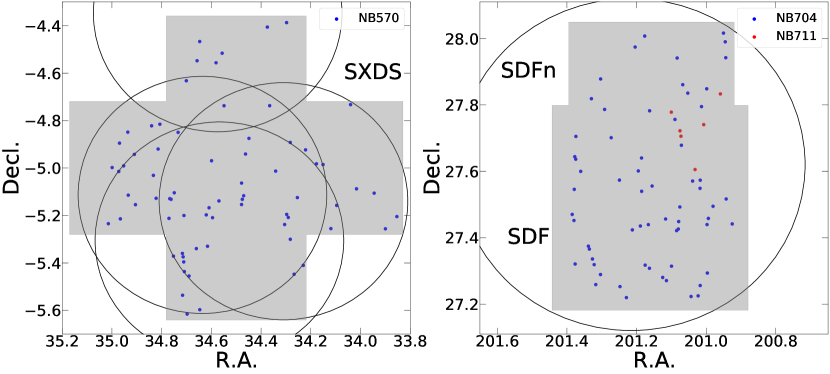
Figure 1: LAEs in the SXDS, SDF, and SDFn fields. The left panel shows LAEs at $z\sim 3.7$ in SXDS and the right panel shows LAEs at $z\sim 4.8$ in SDF and SDFn. In each panel, the grey regions indicate the coverage area of the Subaru Suprime-Cam images. The large circles represent the pointings of our Hectospec observations. The color-coded points represent spectroscopically confirmed LAEs.

High-redshift LAEs are usually young, compact, metal-poor, and low-mass (stellar mass $\sim 10^{8-9}M_{\odot}$) star-forming galaxies with star formation rates around $\sim 1-10\,M_{\odot}/\rm yr$ (2020ARA&A..58..617O). Since the discovery of the first high-redshift LAEs using the narrowband technique (1996Natur.380..411P; 1996Natur.382..231H; 1996Natur.383...45P), this technique has successfully found a large number of LAEs at $z\geq 2$ (e.g., 2008ApJS..176..301O; 2012ApJ...744..110C; 2018MNRAS.476.4725S; 2019ApJ...886...90H; 2020ApJ...902..137G; 2020ApJ...903....4N; 2022ApJ...926..230N). Large samples of LAEs from low to high redshift allow us to study their Ly$\alpha$ luminosity function (LF) and evolution (e.g., 2011A&A...525A.143C; 2017A&A...608A...6D; 2018PASJ...70S..16K; 2019A&A...621A.107H; 2020ApJ...902..137G; 2021ApJ...922..167Z), and physical properties (e.g., 2013ApJ...772...99J; 2016ApJ...816...16J; 2019ApJ...871..164S; 2011ApJ...736..160S). They also allow us to find protoclusters of galaxies (e.g., 2018NatAs...2..962J; 2021NatAs...5..485H) and characterize the end of cosmic reionization (e.g., 2006ApJ...648....7K; 2011ApJ...734..119K; 2022ApJ...926..230N). The recently launched James Webb Space Telescope (JWST) allows us to study their rest-frame optical spectral properties and their correlations with the Ly$\alpha$ line (e.g., 2023arXiv230401437R).

The Ly$\alpha$ LF describes the number density of LAEs as a function of Ly$\alpha$ luminosity, and is thus a basic statistical property of LAEs. Current studies show that the Ly$\alpha$ LF increases rapidly from $z\sim 0.3$ to $z\sim 3$, appears constant from $z\sim 3$ to $z\sim 6$, and then declines rapidly from $z\sim 6$ towards higher redshift (2020ARA&A..58..617O). However, the Ly$\alpha$ LF at $z\sim 4-5$ has not been well explored, and previous studies for this redshift range were mostly based on photometric samples of LAEs. For example, 2003ApJ...582...60O calculated $z\sim 4.86$ Ly$\alpha$ LF using a photometric sample consisting of 87 LAE candiadtes. 2008ApJS..176..301O derived $z\sim 3.7$ Ly$\alpha$ LF based on 101 photometrically selected LAE candidates, and they spectroscopically confirmed 26 LAEs. 2009ApJ...696..546S obtained $z\sim 4.86$ Ly$\alpha$ LF with 79 photometrically selected LAE candidates. There are some studies based on spectroscopic samples, but the number is relatively small. For example, 2013MNRAS.431.3589Z combined results from the Large Area Lyman Alpha (LALA) survey and derived $z\sim 4.5$ Ly$\alpha$ LF based on a large sample of 207 spectroscopically confirmed LAEs. Although the typical confirmation rate of LAE candidates selected by the narrowband technique is high ($\sim 60\%$ to $\sim 80\%$, e.g., 2011ApJ...734..119K; 2013MNRAS.431.3589Z), a spectroscopically confirmed LAE sample is still important in studying Ly$\alpha$ LF by excluding contaminants and deriving more robust Ly$\alpha$ flux.

In this paper, we present spectroscopic surveys of LAEs at $z\sim 3.7$ in the Subaru XMM-Newton Deep Survey (SXDS) field and LAEs at $z\sim 4.8$ in the Subaru Deep Field (SDF). We select LAE candidates from deep broadband and narrowband images taken by the Subaru Suprime-Cam and spectroscopically observe them with the MMT Hectospec spectrograph. From these observations, we obtain large samples of LAEs at $z\sim 3.7$ and $z\sim 4.8$, and we further derive Ly$\alpha$ LFs at the two redshifts. The layout of this paper is as follows. In Section 2, we introduce target selection and spectroscopic observations. In Section 3, we describe LAE samples and properties. Ly$\alpha$ LFs are derived in Section LABEL:sec:laeLF. Section LABEL:sec:discussion and Section LABEL:sec:summary are discussion and summary. Throughout this paper, all magnitudes are in the AB system. We adopt a $\Lambda$-dominated flat cosmology with $H_{0}=70\rm\,km\,s^{-1}\,Mpc^{-1}$, $\Omega_{m}=0.3$, and $\Omega_{\Lambda}=0.7$.

2 Target selection and spectroscopic observations

In this section, we will describe the imaging data in the SXDS and SDF fields, the selection of LAE candidates, the spectroscopic observations of these candidates, and our data reduction.

2.1 Subaru Suprime-Cam images in SXDS and SDF

The Suprime-Cam is a wide-field prime-focus imager with a field-of-view of $34\arcmin\times 27\arcmin$ and a pixel scale of $0.202\arcsec$ per pixel for the 8.2m Subaru telescope. The Subaru XMM-Newton Deep Survey (SXDS, 2008ApJS..176....1F, Figure 1) is centered on ($\rm 02^{h}18^{m}00^{s}$, $-05\arcdeg 00\arcmin 00\arcsec$). It consists of five contiguous subfields SXDS-C, N, S, E, and W (hereafter SXDS1, 2, 3, 4, and 5) corresponding to five Suprime-Cam pointings. The total area coverage is $\sim 1.2$ deg${}^{2}$. The Subaru deep field (SDF, 2004PASJ...56.1011K, Figure 1) is centered on ($\rm 13^{h}24^{m}38\fs 9$, $+27\arcdeg 29\arcmin 25\farcs 9$) and covers an area of $\sim 800$ arcmin${}^{2}$. Suprime-Cam has taken deep images of the SXDS and SDF fields in a series of broad and narrow bands. These images have been widely used to search for high-redshift LBGs and LAEs (e.g., 2006ApJ...653..988Y; 2008ApJS..176..301O; 2006ApJ...648....7K; 2011ApJ...734..119K; 2014ApJ...797...16K; 2016ApJ...823...20K).

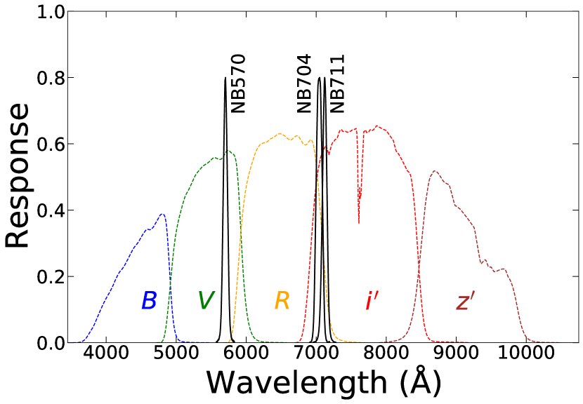
Figure 2: Response curves of the narrowband filters (black solid lines) and broadband filters (dashed lines) used in this work. Instrument response has been included for the broad bands.The maximum responses of the narrowband filters are set to 0.8 for the purpose of clarity. The filter NB570 is used to select $z\sim 3.7$ LAEs, and the NB704 and NB711 filters are used to select $z\sim 4.8$ LAEs.

We retrieved the raw images from the archival server SMOKA (2002ASPC..281..298B). The images were reduced, re-sampled, and co-added using a combination of the Suprime-Cam Deep Field REDuction package (2002AJ....123...66Y) and the IDL routines by 2013ApJ...772...99J. Source extraction and astrometric and photometric solutions were then applied. The details are given in 2013ApJ...772...99J. We performed aperture photometry with SExtractor (1996A&AS..117..393B) in dual-image mode using the narrowband images as the detection images. Aperture photometry was measured in a $2\arcsec$ diameter aperture and an aperture correction was then determined from a large number of bright but unsaturated point sources and applied to correct for light loss. The depths ($5\sigma$ in a $2\arcsec$ diameter aperture) of the imaging data in five broad bands $BVRi^{\prime}z^{\prime}$ reach 27.9, 27.6, 27.4, 27.4, and 26.2 AB mag in SXDS, and 28.0, 27.2, 28.0, 27.8, and 26.8 AB mag in SDF. The typical PSF FWHM of the images is $0.6\arcsec$ in the $i^{\prime}$ band. Galactic extinction was corrected using the $E(B-V)$ values at the center of SXDS and SDF, respectively.

Narrowband imaging data were reduced in the same method. Figure 2 shows the transmission curves of the narrow bands used in this paper. No strong OH sky line lies within the passbands of these narrowband filters. NB570 ($\lambda_{c}=\rm 5703\,\AA$; $\rm FWHM=68\,\AA$) is used to select $z\sim 3.7$ LAE candidates in SXDS. The depth of the NB570 image is about $24.8$ mag and it slightly varies across the five SXDS subfields ($\pm 0.2\rm\,mag$). NB704 ($\lambda_{c}=\rm 7042\,\AA$; $\rm FWHM=99\,\AA$) and NB711 ($\lambda_{c}=\rm 7120\,\AA$; $\rm FWHM=73\,\AA$) are used to select $z\sim 4.8$ LAE candidates in SDF. The depths of the NB704 and NB711 images in SDF are $26.2\rm\,mag$ and $25.5\rm\,mag$, respectively. A smaller region in the north of SDF (hereafter SDFn) also has $R$, $i^{\prime}$, NB704, and NB711-band images with depths of 26.9, 26.5, 26.1, and 25.3 mag, respectively, so $z\sim 4.8$ LAE candidates are also selected in this field.

2.2 Target selection in SXDS and SDF

Based on the filter curves shown in Figure 2 and the positions of the redshifted Ly$\alpha$ emission lines, we apply the following criteria to select LAE candidates at $z\sim 3.7$ and $z\sim 4.8$. These criteria roughly select LAEs with Ly$\alpha$ rest-frame equivalent width $\rm EW_{0}\gtrsim 20\,\AA$.

For $z\sim 3.7$ LAE candidates in SXDS, the Ly$\alpha$ line locates around $\rm 5700\,\AA$, between the $V$ and $R$ bands. The selection criteria are as follows.

(1) $\rm\sigma(NB570)\leq 0.156$ (i.e., $>7\sigma$ detection in NB570) and $\rm NB570>18.0$;

(2) $VR\rm-NB570>0.9$, where $VR$ is an AB magnitude calculated from the $V$ and $R$-band flux: $f_{VR}=0.8\times f_{V}+0.2\times f_{R}$;

(3) $\sigma(V)\leq 0.362$ (i.e., $>3\sigma$ detection in $V$);

(4) $B-V>0.5$.

The above first and second criteria are the major selection criteria. Criteria 3 and 4 are mainly used to remove contaminants without excluding real LAEs at $z\sim 3.7$. For $z\sim 4.8$ LAE candidates in SDF, the Ly$\alpha$ line locates around $\rm 7050\,\AA$, between the $R$ and $i^{\prime}$ bands. There are two narrowband filters NB704 and NB711. The selection criteria are as follows.

(1a) For NB704: $\rm\sigma(NB704)\leq 0.136$ (i.e., $>8\sigma$ detection in NB704) and $\rm 18.0<NB704<25.55$;

(1b) For NB711: $\rm\sigma(NB711)\leq 0.156$ (i.e., $>7\sigma$ detection in NB711) and $\rm NB711>18.0$;

(2) $Ri^{\prime}-\rm NB>0.9$, where $Ri^{\prime}$ is an AB magnitude calculated from the $R$ and $i^{\prime}$-band flux: $f_{Ri^{\prime}}=0.5\times f_{R}+0.5\times f_{i^{\prime}}$;

(3) $\sigma(i^{\prime})\leq 0.362$ (i.e., $>3\sigma$ detection in $i^{\prime}$);

(4) $\sigma(B)>0.362$ or $\sigma(V)>0.362$ or $B-i^{\prime}>2.0$.

Like for the $z\sim 3.7$ LAE candidates, the above first and second criteria are the major selection criteria, and Criteria 3 and 4 are used to remove contaminants without excluding real LAEs at $z\sim 4.8$. The selection criteria for $z\sim 4.8$ LAE candidates in SDFn are as follows (only $R$, $i^{\prime}$, NB704, and NB711-band images are available).

(1a) For NB704: $\rm\sigma(NB704)\leq 0.136$ (i.e., $>8\sigma$ detection in NB704) and $\rm 20.0<NB704<25.55$;

(1b) For NB711: $\rm\sigma(NB711)\leq 0.156$ (i.e., $>7\sigma$ detection in NB711) and $\rm NB711>20.0$;

(2) $Ri^{\prime}-\rm NB>0.9$, where $Ri^{\prime}$ is an AB magnitude calculated from the $R$ and $i^{\prime}$-band flux: $f_{Ri^{\prime}}=0.5\times f_{R}+0.5\times f_{i^{\prime}}$;

(3) $\sigma(r)>0.362$ or $r-i^{\prime}>0.1$.

In the above selection procedure, we used slightly different narrowband detection limits ($7\sigma$ or $8\sigma$) for different fields. This is to optimize the target surface densities for follow-up spectroscopy, because different narrowband images have different depths. The selected LAE candidates were visually inspected to exclude spurious detections, such as those near the edges of the narrowband images and those contaminated by nearby bright stars. Finally, we selected 112 $z\sim 3.7$ LAE candidates in the NB570 image of SXDS, 123 $z\sim 4.8$ LAE candidates in the NB704 images of SDF (87) and SDFn (36), and 28 $z\sim 4.8$ LAE candidates in the NB711 images of SDF (16) and SDFn (12).

Table 1: Summary of the MMT Hectospec observations.

Date	Grating	Center (R.A., Decl.)	Exp. Time	No.
		$z\sim 3.7$
2017.09.28	600	$\rm 02^{h}18^{m}33^{s},-05\arcdeg 06\arcmin 48\arcsec$	120 min	64
2017.09.28	600	$\rm 02^{h}18^{m}33^{s},-05\arcdeg 06\arcmin 48\arcsec$	60 min	45
2017.10.01	600	$\rm 02^{h}18^{m}33^{s},-05\arcdeg 06\arcmin 48\arcsec$	90 min	64
2020.10.11	270	$\rm 02^{h}17^{m}14^{s},-05\arcdeg 08\arcmin 24\arcsec$	200 min	22
2021.10.03	270	$\rm 02^{h}18^{m}16^{s},-05\arcdeg 18\arcmin 21\arcsec$	180 min	9
2021.12.08	270	$\rm 02^{h}18^{m}18^{s},-04\arcdeg 20\arcmin 50\arcsec$	225 min	14
		$z\sim 4.8$
2018.05.19	600	$\rm 13^{h}24^{m}52^{s},+27\arcdeg 37\arcmin 14\arcsec$	80 min	72
2019.04.27	600	$\rm 13^{h}24^{m}52^{s},+27\arcdeg 37\arcmin 14\arcsec$	240 min	71

2.3 Spectroscopic observations and data reduction

We carried out follow-up spectroscopic observations of these LAE candidates from 2017 to 2021, using the optical fiber-fed spectrograph Hectospec on the $\rm 6.5\,m$ telescope MMT (2005PASP..117.1411F). Hectospec has a large field-of-view of $1\arcdeg$ in diameter with 300 fibers. The diameter of each fiber is $1\farcs 5$ and adjacent fibers can be spaced as closely as $20\arcsec$. The observations are summarized in Table 1.

We observed the $z\sim 3.7$ LAE candidates in SXDS using four Hectospec pointings with two different configurations. This is because many fibers were shared by other projects. In 2017, we used the $\rm 600\,lines\,mm^{-1}$ grating blazed at $\rm\sim 6000\,\AA$, providing a spectral resolution of $\rm\sim 2.1\,\AA$ and a wavelength coverage from $\rm 4050\,\AA$ to $\rm 6550\,\AA$. In 2020 and 2021, we used the $\rm 270\,lines\,mm^{-1}$ grating blazed at $\rm\sim 5000\,\AA$, providing a spectral resolution of $\rm\sim 4.8\,\AA$ and a wavelength coverage from $\rm 3650\,\AA$ to $\rm 9200\,\AA$. For the $z\sim 4.8$ LAE candidates in SDF and SDFn, one Hectospec pointing was use to cover most of the sky area. They were observed in 2018 and 2019 with the $\rm 600\,lines\,mm^{-1}$ grating that covered a wavelength coverage from $\rm 6050\,\AA$ to $\rm 8550\,\AA$. The seeing of these observations varied from $\sim 0.7\arcsec$ to $\sim 1.5\arcsec$. For each pointing, about 80 fibers were assigned to blank sky regions for background subtraction.

All $z\sim 4.8$ LAE candidates and all but one $z\sim 3.7$ LAE candidates were covered by the above Hectospec pointings, and the only one $z\sim 3.7$ LAE candidate out of the pointings is excluded in the following analyses. The effective areas of the SXDS sub-fields SXDS1, 2, 3, 4, 5 covered by the pointings are 0.232, 0.235, 0.235, 0.167, and $\rm 0.181\,deg^{2}$, respectively. The total effective area in SXDS is $\rm 1.050\,deg^{2}$. The effective areas in SDF and SDFn covered by the pointings are 0.279 and $\rm 0.125\,deg^{2}$, respectively, with a total area of $\rm 0.404\,deg^{2}$. Due to the fiber collision, not all candidates were spectroscopically observed. In summary, 99 out of 112 $z\sim 3.7$ LAE candidates, 96 out of 123 $z\sim 4.8$ LAE candidates in NB704, and 12 out of 28 $z\sim 4.8$ LAE candidates in NB711 were spectroscopically observed. The total exposure time for each target varies from $\rm 1\,h$ to $\rm 7\,h$. This complexity is partly due to the fact that the fibers were shared by different programs, as mentioned earlier. However, our observing strategy ensures that fainter LAE candidates were assigned with longer exposure time so that their Ly$\alpha$ emission lines can be identified if they are real LAEs.

The Hectospec data were processed and reduced using the HSRED reduction pipeline. For each exposure, science and lamp images were bias subtracted, flat-fielded, and cosmic ray rejected. Each fiber was traced, and each one-dimensional (1D) spectrum was extracted. Wavelength solution was then derived. Sky spectrum from each sky fiber was checked and poor sky spectra were rejected. An average “supersky” spectrum was obtained from good sky spectra, which was then scaled according to the strength of skylines in individual object’s spectrum and subtracted from it. The resultant 1D, sky-subtracted, and wavelength-calibrated spectra for different exposures of the same object were then re-sampled to the same wavelength grid and co-added with inverse variance weighting to achieve the final 1D spectrum.

3 LAE samples and their properties at $z\sim 3.7$ and $z\sim 4.8$

In this section, we construct the spectroscopic samples of LAEs at $z\sim 3.7$ and $z\sim 4.8$. We then derive their spectral properties, including redshift, UV continuum flux, and Ly$\alpha$ line flux and EW.

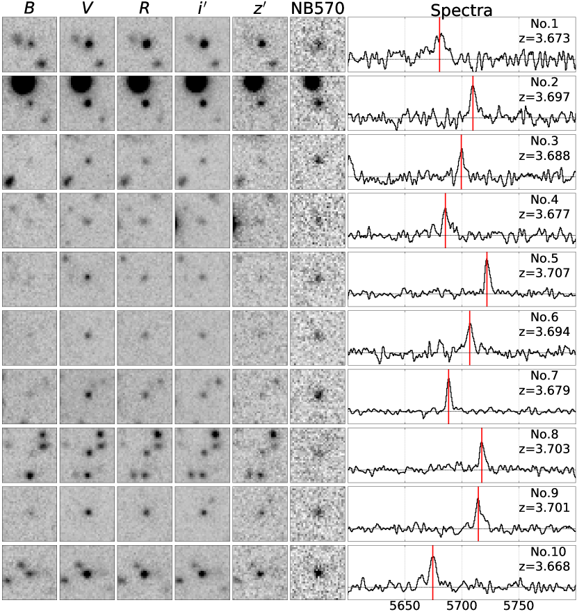
Figure 3: Example of 10 LAEs spectroscopically identified at $z\sim 3.7$. The left panel shows the stamp images in five broad bands and the narrowband NB570. The image size is $6\arcsec\times 6\arcsec$. The right panel shows the optical spectra of the LAEs taken by MMT Hectospec. The red vertical lines indicate the positions of the redshifted Ly$\alpha$ lines. A figure of the full version is shown in the Appendix.

3.1 LAE samples

We identify LAEs as follows. For each 1D spectrum, we first search for a possible emission line in the wavelength range covered by the narrowband filters. If a line with signal-to-noise ratio SNR$>5$ is detected, this object is regarded as a possible LAE. Low-redshift interlopers are mostly likely [O II] $\lambda\lambda 3727,3729$, [O III] $\lambda\lambda 4959,5007$, or H$\beta$ emitters. H$\alpha$ emitters are also possible for $z\sim 4.8$ candidates. These contaminants are identified and excluded using the following steps. If an emission line is [O III], H$\beta$, or H$\alpha$, the spectrum would cover more than one of these lines, and such an interloper can be easily identified. If an emission line is [O II] and if the spectrum was taken by the $\rm 270\,lines\,mm^{-1}$ grating, the spectrum would cover [O III], H$\beta$, and H$\alpha$, and thus the line is easy to identify. If the spectrum was taken by the $\rm 600\,lines\,mm^{-1}$ grating, the wavelength coverage is short, but the spectral resolution is higher enough to identify the [O II] doublet. In rare cases, a Ly$\alpha$ line profile can also exhibit a double-peak feature (e.g., 2006A&A...460..397V), which mimics the [O II] doublet if its SNR is low. In this case, Ly$\alpha$ and [O II] can be distinguished using the broadband photometry, given the fact the two redshifts would be very different. If the SNR is high, they can be immediately distinguished by the line profile.

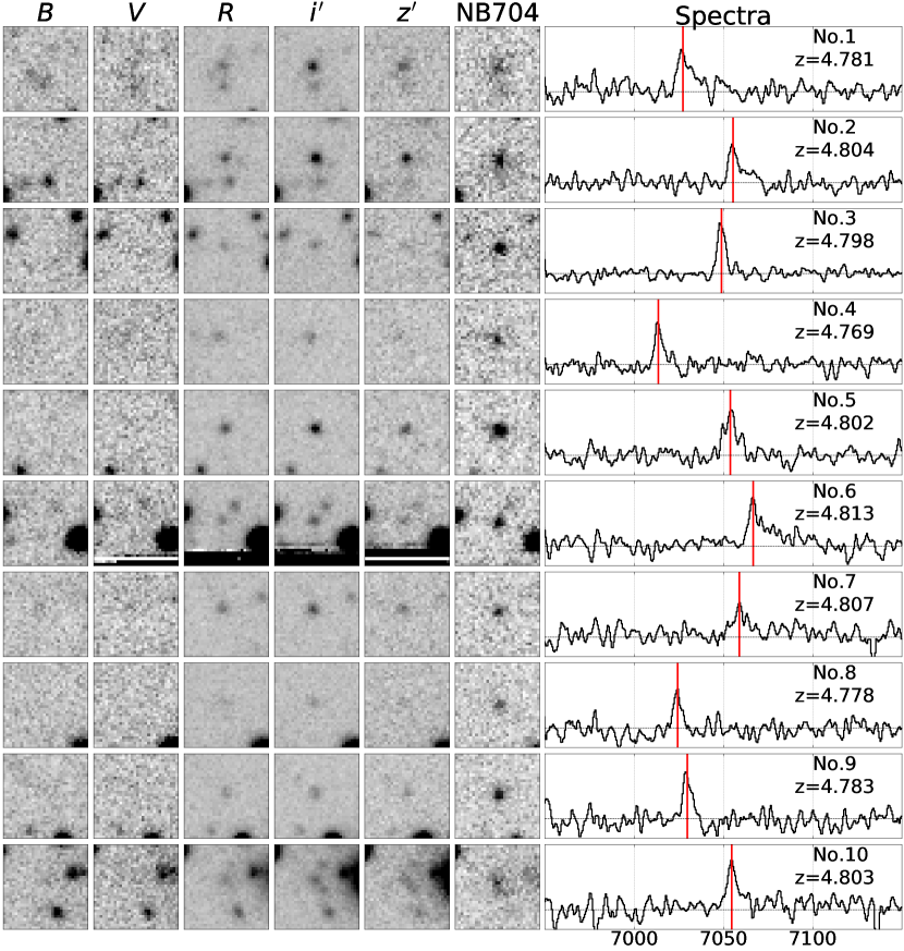
Figure 4: Same as Figure 3, but for our $z\sim 4.8$ LAEs selected in NB704. A figure of the full version is shown in the Appendix.

Active galactic nuclei (AGNs) are also identified and excluded. For the $z\sim 3.7$ LAE candidates in SXDS, deep X-ray images taken by Chandra (2018ApJS..236...48K) and XMM-Newton (2018MNRAS.478.2132C) are available. If an object is detected in X-ray, it is considered as an AGN. In addition, if an object has broad emission lines (line FWHM greater than 1000 km $s^{-1}$) in the spectra, it is also considered as an AGN. One X-ray AGN and one broad-line AGN are identified in our sample. For the $z\sim 4.8$ LAE candidates in SDF and SDFn, there are no X-ray data available, and AGNs are identified based on broad emission lines in the spectra. We find 2 AGNs in our $z\sim 4.8$ sample. Thus, the AGN fractions in narrowband selected, LAE photometric samples at both $z\sim 3.7$ ($2/99$) and $z\sim 4.8$ ($2/(96+12)=2/108$) are around $2\%$, which is consistent with the value reported in previous studies at similar redshifts (e.g., 2008ApJS..176..301O).

Interestingly, we find that one $z\sim 4.8$ LAE candidate ($\rm 13^{h}25^{m}32\fs 73,+27\arcdeg 41\arcmin 34\farcs 4$) is a supernova (SN) happened in 2001 in a host galaxy at $z=0.515$ (see Figure 7 in 2010PASJ...62...19M). This object was selected as a LAE candidate because the narrowband image (NB711) was taken in 2001 about one month after the maximum light of the SN, while the broadband images were all taken after 2002 so that the broadband magnitudes were fainter.

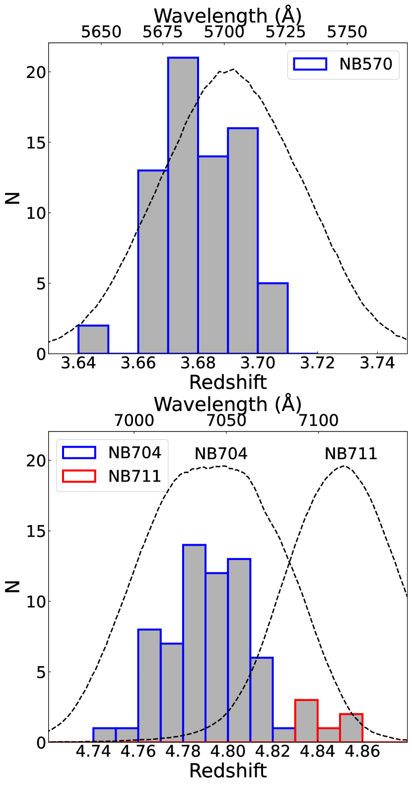
Figure 5: Redshift distribution of the spectroscopically confirmed LAEs at $z\sim 3.7$ (upper panel) and $z\sim 4.8$ (lower panel). The dashed lines show the response curves of the narrowband filters.

From the above procedure, 71 $z\sim 3.7$ LAEs and 69 $z\sim 4.8$ LAEs (including 63 NB704-selected LAEs and 6 NB711-selected LAEs) are spectroscopically confirmed. In the remaining 28 (39) objects at $z\sim 3.7$ ($4.8$), we find 1 (3) low-redshift [O II] emitters, 10 (2) low-redshift [O III] emitters, and 2 (2) AGNs. In addition, 15 (32) objects do not have SNR$>5$ emission lines in the spectra, and they are likely red stars/galaxies, transients, or spurious detections. In the following analysis, only the confirmed LAEs are considered. Their spatial distributions are shown as the blue and red points in Figure 1. Figures 3 presents the stamp images and spectra of the confirmed $z\sim 3.7$ LAEs. Figures 4 presents the stamp images and spectra of the confirmed $z\sim 4.8$ LAEs. Properties of these LAEs are listed in Table 2 and Table 3.

Table 2: Properties of the $z\sim 3.7$ LAEs

No.	R.A.	Decl.	$B$	$V$	$R$	$i^{\prime}$	$z^{\prime}$	NB	Redshift	$\log_{10}(L_{\rm Ly\alpha})$	$\rm EW_{0}$	$\rm M_{UV}$
	(J2000)	(J2000)	(mag)	(mag)	(mag)	(mag)	(mag)	(mag)		($\rm erg~{}s^{-1}$)	($\rm\AA$)	(mag)
1	02:18:59.81	$-$05:06:15.7	25.95	24.76	24.38	24.37	24.41	23.62	3.673	$42.92_{-0.07}^{+0.06}$	$23.2_{-3.5}^{+3.9}$	$-21.50_{-0.01}^{+0.01}$
2	02:18:26.24	$-$05:10:03.5	25.76	24.70	24.62	24.61	24.49	23.31	3.697	$43.10_{-0.03}^{+0.03}$	$47.6_{-3.8}^{+4.2}$	$-21.28_{-0.01}^{+0.01}$
3	02:18:23.83	$-$04:58:09.5	$>$28.46	26.29	26.59	26.60	$>$26.91	23.97	3.688	$42.88_{-0.05}^{+0.05}$	$135.7_{-38.7}^{+54.4}$	$-19.27_{-0.10}^{+0.09}$
4	02:18:16.69	$-$05:08:19.6	27.98	26.15	26.26	26.13	25.98	24.25	3.677	$42.81_{-0.07}^{+0.07}$	$117.0_{-25.1}^{+30.6}$	$-19.68_{-0.06}^{+0.06}$
5	02:17:54.88	$-$05:09:14.0	27.84	25.83	26.48	26.43	$>$26.91	24.12	3.707	$42.92_{-0.06}^{+0.05}$	$116.9_{-35.5}^{+48.3}$	$-19.39_{-0.08}^{+0.08}$
6	02:17:54.86	$-$05:03:48.5	27.92	26.24	26.39	26.36	26.11	24.12	3.695	$42.83_{-0.06}^{+0.05}$	$138.6_{-26.2}^{+32.0}$	$-19.53_{-0.07}^{+0.07}$
7	02:17:54.09	$-$05:07:55.0	27.61	25.65	26.05	26.11	26.66	23.52	3.679	$43.09_{-0.04}^{+0.03}$	$119.7_{-26.5}^{+33.0}$	$-19.77_{-0.05}^{+0.05}$
8	02:17:52.79	$-$05:07:00.4	27.34	25.60	25.77	25.71	25.84	24.21	3.703	$42.81_{-0.07}^{+0.06}$	$62.2_{-11.3}^{+13.6}$	$-20.14_{-0.04}^{+0.04}$
9	02:17:51.03	$-$04:56:27.6	27.11	25.56	25.63	25.62	25.46	23.81	3.701	$42.97_{-0.05}^{+0.04}$	$90.9_{-12.4}^{+14.0}$	$-20.28_{-0.04}^{+0.04}$
10	02:17:21.95	$-$05:00:46.8	25.86	24.76	24.74	24.76	24.77	23.27	3.668	$43.26_{-0.03}^{+0.03}$	$72.2_{-6.4}^{+7.1}$	$-21.13_{-0.01}^{+0.01}$
11	02:17:11.29	$-$05:11:44.2	27.21	25.72	25.51	25.50	25.26	24.09	3.689	$42.78_{-0.07}^{+0.07}$	$54.7_{-9.7}^{+11.6}$	$-20.40_{-0.03}^{+0.03}$
12	02:17:07.85	$-$04:53:32.0	26.00	25.13	25.16	25.07	25.09	23.96	3.676	$42.85_{-0.07}^{+0.07}$	$41.5_{-6.9}^{+7.9}$	$-20.75_{-0.02}^{+0.02}$
13	02:17:01.01	$-$05:07:28.8	27.89	26.42	26.99	26.64	26.81	24.12	3.686	$42.83_{-0.06}^{+0.06}$	$211.0_{-64.8}^{+92.2}$	$-19.02_{-0.12}^{+0.12}$
14	02:18:48.17	$-$04:37:55.3	26.64	25.24	25.18	25.17	25.32	23.83	3.660	$43.15_{-0.05}^{+0.05}$	$77.3_{-11.1}^{+12.2}$	$-20.69_{-0.02}^{+0.02}$
15	02:18:11.77	$-$04:44:14.6	26.99	25.58	25.60	25.60	25.79	24.01	3.667	$42.98_{-0.06}^{+0.05}$	$76.3_{-13.3}^{+15.5}$	$-20.27_{-0.04}^{+0.04}$
16	02:17:27.72	$-$04:44:13.9	27.52	25.87	25.62	25.60	25.63	24.02	3.685	$42.81_{-0.05}^{+0.05}$	$57.2_{-8.8}^{+9.9}$	$-20.27_{-0.04}^{+0.04}$
17	02:19:00.61	$-$05:22:17.7	$>$28.76	27.53	27.75	27.35	$>$26.76	24.49	3.690	$42.70_{-0.06}^{+0.06}$	$429.2_{-181.7}^{+308.7}$	$-18.33_{-0.25}^{+0.25}$
18	02:18:51.95	$-$05:21:36.1	$>$28.76	26.78	27.21	27.37	$>$26.76	24.47	3.672	$42.81_{-0.06}^{+0.06}$	$306.9_{-111.7}^{+171.6}$	$-18.63_{-0.18}^{+0.18}$
19	02:18:51.79	$-$05:32:10.9	26.15	24.73	24.47	24.44	24.34	23.42	3.671	$43.11_{-0.03}^{+0.03}$	$42.7_{-3.6}^{+3.8}$	$-21.42_{-0.01}^{+0.01}$
20	02:18:51.24	$-$05:22:28.5	26.53	24.98	24.65	24.50	24.55	23.80	3.672	$42.89_{-0.06}^{+0.05}$	$28.8_{-4.2}^{+4.4}$	$-21.28_{-0.02}^{+0.02}$

Note. — Col.(1): LAE numbers. Cols.(2)-(3): R.A. and Decl. Cols.(4)-(9): magnitudes in broadband $B$, $V$, $R$, $i^{\prime}$, $z^{\prime}$ and in narrowband NB570; $2\sigma$ upper limits are shown if fainter than a $2\sigma$ detection in the filter. Col.(10): redshifts measured from the Ly$\alpha$ line. Col.(11): logarithm of Ly$\alpha$ luminosity in units of $\rm erg~{}s^{-1}$. Col.(12): rest-frame equivalent width of the Ly$\alpha$ emission line. Col.(13): UV magnitudes at rest-frame 1500$\rm\AA$. Objects without $L_{\rm Ly\alpha}$, $\rm EW_{0}$, and $\rm M_{UV}$ are affected by nearby objects in their narrow- and broadband photometry. The table only shows the first 20 $z\sim 3.7$ LAEs. A full table is available in the electronic version.

3.2 Ly$\alpha$ redshifts

We calculate the redshifts of the LAEs using the Ly$\alpha$ emission lines. For each LAE, its redshift is determined by fitting a composite Ly$\alpha$ line profile to the Ly$\alpha$ line in its spectrum. The composite Ly$\alpha$ line profile is obtained as follows. We first assume that the peak of the Ly$\alpha$ line is at $\rm 1215.67\,\AA$ in the rest frame, and transform all spectra into the rest frame. We then take the average of all spectra to construct a composite Ly$\alpha$ line profile. When we fit the composite line profile to the individual Ly$\alpha$ lines, we vary its redshift and amplitude. After obtaining new redshifts from the fitting results, we use them to transform the spectra into the rest frame again. We repeat the above procedure a few times. The final products include the average Ly$\alpha$ line profiles at $z\sim 3.7$ and $z\sim 4.8$ and redshifts for all our LAEs. Because the Ly$\alpha$ line is typically redshifted compared with other strong emission lines (e.g., 2003ApJ...588...65S; 2021MNRAS.505.1382M), possibly due to the back scattering of Ly$\alpha$ photons in outflowing gas (e.g., 2006A&A...460..397V), Ly$\alpha$ redshifts derived from the Ly$\alpha$ line are higher than systemic redshifts.

Table 3: Properties of the $z\sim 4.8$ LAEs

No.	R.A.	Decl.	$B$	$V$	$R$	$i^{\prime}$	$z^{\prime}$	NB	Redshift	$\log_{10}(L_{\rm Ly\alpha})$	$\rm EW_{0}$	$\rm M_{UV}$
	(J2000)	(J2000)	(mag)	(mag)	(mag)	(mag)	(mag)	(mag)		($\rm erg~{}s^{-1}$)	($\rm\AA$)	(mag)
1	13:25:32.38	$+$27:28:13.0	28.35	27.20	26.49	25.76	25.65	25.08	4.781	$42.48_{-0.07}^{+0.07}$	$20.7_{-3.7}^{+4.0}$	$-20.52_{-0.05}^{+0.05}$
2	13:25:31.17	$+$27:27:07.3	$>$28.76	$>$28.20	26.46	25.53	25.47	24.62	4.804	$42.78_{-0.04}^{+0.04}$	$34.5_{-3.3}^{+3.7}$	$-20.71_{-0.04}^{+0.04}$
3	13:25:30.95	$+$27:32:44.8	$>$28.76	$>$28.20	27.72	27.27	27.52	24.78	4.798	$42.80_{-0.03}^{+0.03}$	$441.0_{-158.9}^{+326.2}$	$-17.99_{-0.43}^{+0.58}$
4	13:25:30.61	$+$27:38:39.2	$>$28.76	$>$28.20	28.03	27.24	27.64	25.07	4.769	$42.72_{-0.05}^{+0.05}$	$253.4_{-81.0}^{+154.6}$	$-18.39_{-0.34}^{+0.45}$
5	13:25:30.36	$+$27:19:15.5	$>$28.76	$>$28.20	26.74	25.90	26.07	24.18	4.802	$43.02_{-0.02}^{+0.02}$	$106.8_{-10.2}^{+11.5}$	$-20.09_{-0.08}^{+0.08}$
6	13:25:29.95	$+$27:38:11.7	$>$28.76	$>$28.20	26.83	26.08	26.11	25.08	4.813	$42.68_{-0.05}^{+0.05}$	$46.7_{-6.9}^{+8.3}$	$-20.12_{-0.09}^{+0.09}$
7	13:25:29.83	$+$27:42:18.6	$>$28.76	$>$28.20	27.07	26.29	26.48	25.39	4.807	$42.49_{-0.06}^{+0.06}$	$35.5_{-5.8}^{+7.2}$	$-19.95_{-0.07}^{+0.08}$
8	13:25:26.49	$+$27:35:59.7	$>$28.76	$>$28.20	27.92	27.44	$>$27.78	25.49	4.778	$42.50_{-0.06}^{+0.06}$	$144.6_{-40.6}^{+64.5}$	$-18.44_{-0.27}^{+0.32}$
9	13:25:21.23	$+$27:22:29.0	$>$28.76	$>$28.20	27.47	26.95	26.86	24.96	4.783	$42.71_{-0.04}^{+0.03}$	$153.6_{-29.9}^{+39.2}$	$-18.90_{-0.19}^{+0.20}$
10	13:25:20.55	$+$27:21:57.1	$>$28.76	$>$28.20	26.51	25.78	25.55	24.97	4.803	$42.63_{-0.04}^{+0.04}$	$30.0_{-3.3}^{+3.7}$	$-20.48_{-0.05}^{+0.05}$
11	13:25:18.41	$+$27:20:09.8	$>$28.76	$>$28.20	27.40	26.42	26.95	24.84	4.799	$42.74_{-0.03}^{+0.03}$	$84.7_{-10.4}^{+13.1}$	$-19.64_{-0.10}^{+0.11}$
12	13:25:17.24	$+$27:19:08.5	$>$28.76	28.11	26.65	25.80	25.81	24.46	4.787	$42.86_{-0.02}^{+0.02}$	$57.1_{-4.8}^{+5.1}$	$-20.35_{-0.05}^{+0.05}$
13	13:25:16.12	$+$27:15:32.3	28.60	$>$28.20	27.55	27.47	$>$27.78	25.45	4.780	$42.51_{-0.06}^{+0.06}$	$160.5_{-49.7}^{+84.5}$	$-18.37_{-0.31}^{+0.37}$
14	13:25:12.86	$+$27:17:21.3	$>$28.76	$>$28.20	27.17	26.48	$>$27.78	24.78	4.798	$42.77_{-0.03}^{+0.03}$	$100.0_{-13.8}^{+17.0}$	$-19.53_{-0.12}^{+0.12}$
15	13:25:05.49	$+$27:42:04.7	27.35	27.95	26.67	26.16	26.04	25.40	4.778	…	…	…
16	13:24:59.81	$+$27:34:24.9	$>$28.76	$>$28.20	26.97	25.87	26.17	25.00	4.812	$42.69_{-0.04}^{+0.04}$	$38.1_{-4.1}^{+4.5}$	$-20.36_{-0.05}^{+0.05}$
17	13:24:59.44	$+$27:15:10.3	$>$28.76	$>$28.20	27.18	26.41	26.35	24.69	4.773	$42.82_{-0.03}^{+0.03}$	$107.1_{-15.7}^{+18.8}$	$-19.58_{-0.12}^{+0.13}$
18	13:24:55.03	$+$27:13:11.0	$>$28.76	$>$28.20	26.95	26.24	25.89	24.73	4.778	…	…	…
19	13:24:50.89	$+$27:25:25.2	$>$28.76	$>$28.20	27.59	26.87	27.23	25.12	4.793	$42.63_{-0.04}^{+0.04}$	$105.9_{-18.0}^{+22.0}$	$-19.12_{-0.14}^{+0.14}$
20	13:24:46.81	$+$27:36:04.2	$>$28.76	$>$28.20	27.63	26.97	27.07	25.31	4.802	$42.57_{-0.04}^{+0.04}$	$96.9_{-17.3}^{+22.3}$	$-19.05_{-0.15}^{+0.16}$

Note. — Col.(1): LAE numbers. Cols.(2)-(3): R.A. and Decl. Cols.(4)-(9): magnitudes in broadband $B$, $V$, $R$, $i^{\prime}$, $z^{\prime}$ and in narrowband NB704 or NB711; $2\sigma$ upper limits are shown if fainter than a $2\sigma$ detection in the filter. Col.(10): redshifts measured from the Ly$\alpha$ line. Col.(11): logarithm of Ly$\alpha$ luminosity in units of $\rm erg~{}s^{-1}$. Col.(12): rest-frame equivalent width of the Ly$\alpha$ emission line. Col.(13): UV magnitudes at rest-frame 1500$\rm\AA$. Objects without $L_{\rm Ly\alpha}$, $\rm EW_{0}$, and $\rm M_{UV}$ are affected by nearby objects in their narrow- and broadband photometry. The table only shows the properties of the first 20 $z\sim 4.8$ LAEs. A full table is available in the electronic version.