On $O(n)$ Algorithms for Projection onto the Top-$k$-sum Constraint

Abstract

The top-$k$-sum operator computes the sum of the largest $k$ components of a given vector. The Euclidean projection onto the top-$k$-sum constraint serves as a crucial subroutine in iterative methods to solve composite superquantile optimization problems. In this paper, we introduce a solver that implements two finite-termination algorithms to compute this projection. Both algorithms have complexity $O(n)$ when applied to a sorted $n$-dimensional input vector, where the absorbed constant is independent of $k$. This stands in contrast to the existing grid-search-inspired method that has $O(k(n-k))$ complexity. The improvement is significant when $k$ is linearly dependent on $n$, which is frequently encountered in practical superquantile optimization applications. In instances where the input vector is unsorted, an additional cost is incurred to (partially) sort the vector. To reduce this cost, we further derive a rigorous procedure that leverages approximate sorting to compute the projection, which is particularly useful when solving a sequence of similar projection problems. Numerical results show that our methods solve problems of scale $n=10^{7}$ and $k=10^{4}$ within $0.05$ seconds, whereas the existing grid-search-based method and the Gurobi QP solver can take minutes to hours.

Keywords: projection, top-$k$-sum, superquantile, $Z$-matrix

1 Introduction

We consider the Euclidean projection onto the top-$k$-sum (also referred to as max-$k$-sum in various works such as [todd2018max, eigen2021topkconv, cucala2023correspondence]) constraint. Specifically, given a scalar budget $r\in\mathbb{R}$, an index $k\in\{1,2,\ldots,n\}$, and an input vector $x^{0}\in\mathbb{R}^{n}$, our aim is to develop a fast and finite-termination algorithm to obtain the exact solution of the strongly convex problem

$$\begin{array}[]{rl}\displaystyle\operatornamewithlimits{minimize}_{x\in\mathbb{R}^{n}}&\displaystyle\frac{1}{2}\lVert x-x^{0}\rVert^{2}_{2}\\ \mbox{subject to}&x\in\mathcal{B}^{r}_{(k)}\coloneqq\bigl{\{}x\in\mathbb{R}^{n}:\displaystyle\mathsf{T}_{(k)}(x)\coloneqq\sum_{i=1}^{k}\reflectbox{$\vec{\reflectbox{$x$}}$}_{i}\leq r\bigr{\}},\end{array}$$ (1)

where for any $x\in\mathbb{R}^{n}$, we write $\reflectbox{$\vec{\reflectbox{$x$}}$}\in\mathbb{R}^{n}$ as its sorted counterpart satisfying $\reflectbox{$\vec{\reflectbox{$x$}}$}_{1}\geq\reflectbox{$\vec{\reflectbox{$x$}}$}_{2}\geq\cdots\geq\reflectbox{$\vec{\reflectbox{$x$}}$}_{n}$, such that $\mathsf{T}_{(k)}(x)$ represents the sum of the largest $k$ elements of $x$.

The top-$k$-sum operator $\mathsf{T}_{(k)}(\bullet)$ is closely related to the superquantile of a random variable, which is also known as the conditional value-at-risk (CVaR) [rockafellar1999cvar], average-top-$k$ [hu2023rank], expected shortfall, among other names. Specifically, consider $X$ as a random variable. Its superquantile at confidence level $\tau\in(0,1)$ is defined as $\mathsf{S}_{\tau}(X)\coloneqq\mathbb{E}[X\,|\,X>\mathsf{Q}_{\tau}(X)]$, i.e., the tail expectation exceeding the $\tau^{\text{th}}$ quantile $\mathsf{Q}_{\tau}(X)\coloneqq\inf\{p\in\mathbb{R}:\mathbb{P}[X\leq p]\geq\tau\}$. When $X$ is supported on $n$ atoms $x\coloneqq(x_{1},\ldots,x_{n})^{\top}$, each with equal probability, then $\mathsf{T}_{(k)}(x)/k=\mathsf{S}_{\tau(k)}(X)$ averages the largest $k$ realizations of $X$, where $\tau(k)\coloneqq 1-k/n$. In the context where $X$ follows a continuous distribution, one may select $n$ samples $x=\{x_{i}\}_{i=1}^{n}$ and construct an empirical sample average approximation of its superquantile using $\mathsf{T}_{(k)}(x)$. Since the superquantile is a coherent risk measure [artzner1999coherent], its translation invariance property facilitates the expression of the top-$k$-sum of $x$ as the top-$k$-sum of a shifted, nonnegative vector $\hat{x}$. Consequently, algorithms designed to solve the top-$k$-sum projection problem may, with minor modifications, also be employed to solve the vector-$k$-norm [wu2014moreau, pavlikov2014cvarnorm] projection problem.

Owing to the close relationship between the top-$k$-sum and the superquantile, the projection problem in (1) has wide applicability as a subroutine in solving composite optimization problems of the form

$$\begin{array}[]{rl}\displaystyle\operatornamewithlimits{minimize}_{z\in Z\subseteq\mathbb{R}^{m}}&\displaystyle f(z)+\mathsf{S}_{\tau_{0}}\big{(}G^{\,0}(z;\omega^{0})\big{)}\\[3.61371pt] \mbox{subject to}&\mathsf{S}_{\tau_{i}}\big{(}G^{\,i}(z;\omega^{i})\big{)}\leq r_{i},\;i\in\{1,2,\ldots,I\},\end{array}$$ (2)

where $Z$ is a given constraint set in $\mathbb{R}^{m}$; $f:\mathbb{R}^{m}\to\mathbb{R}$ is a scalar-valued function; for each $i\in\{0,1,\ldots,I\}$, $\tau_{i}\in(0,1)$ and $r_{i}\in\mathbb{R}$ are given scalars, and the notation $\omega^{i}\coloneqq\{\omega^{i,j}\}_{j=1}^{n_{i}}\subseteq\mathbb{R}^{m_{i}}$ signifies a collection of $n_{i}$ samples from the $i^{\text{th}}$ random vector in $\mathbb{R}^{m_{i}}$. Furthermore, each $G^{\,i}\coloneqq(g^{\,i}(z;\omega^{i,j}))_{j=1}^{n_{i}}:\mathbb{R}^{m}\times\mathbb{R}^{m_{i}}\to\mathbb{R}^{n_{i}}$ defines a vector-valued function, with the $j^{\text{th}}$ entry $g^{\,i}(z;\omega^{i,j})$ representing the random function $g^{\,i}(z;\bullet)$ evaluated at the $j^{\text{th}}$ sample $\omega^{i,j}$. Problem (2) covers the empirical version or the sample average approximation of risk-averse CVaR problems, which is often employed in safety-critical applications where careful control over adverse outcomes is needed, such as the robust design of complex systems [dahlgren2003risk, dolatabadi2017stochastic, tavakoli2018resilience, rabih2020distributionally, chaudhuri2022certifiable]. Additionally, such a problem arises from the convex approximation of chance constrained stochastic programs [nemirovski2006convex, chen2010cvar], and is relevant to matrix optimization problems involving a matrix’s Ky-Fan norm [overton1993optimality, wu2014moreau], i.e., the vector-$k$-norm of its (already sorted) singular values. Recently, optimization problems involving superquantiles have attracted significant attention in the machine learning community, proving instrumental in modeling problems which: (i) seek robustness against uncertainty, such as mitigating distributional shifts between training and test datasets [laguel2021superquantiles], or measuring robustness through probabilistic guarantees on solution quality [robey2022probabilistic]; (ii) handle imbalanced data [yuan2020group, peng2022imbalanced]; or (iii) pursue notions of fairness [williamson2019fairness, frohlich2022risk, liu2019human]. Interested readers are encouraged to consult a recent survey [royset2022risk] for a comprehensive review of superquantiles. A fast and reliable solver for computing the projection onto the top-$k$-sum constraint, especially when dealing with a large number of samples $\{n_{i}\}_{i=0}^{I}$, is crucial for numerous first- or second-order methods to solve the large-scale, complex composite problem (2).

Given that problem (1) is a strongly convex quadratic program, it accommodates the straightforward utilization of off-the-shelf solvers, such as Gurobi, to compute its solution. However, results from our numerical experiments indicate that Gurobi needs about $1$-$2$ minutes at best to solve problems of size $n=10^{7}$, thus preventing its usage as an effective subroutine within an iterative solver to solve the composite problem (2); see Table 1 in Section 4 for details of the numerical results. In addition to their lack of scalability, generic quadratic programming solvers yield inexact solutions, which can lead to: (i) an accumulation of errors, potentially impeding convergence of iterative methods to solve the overall composite problem; and (ii) a challenge in precisely determining the (generalized) Jacobian associated with the projection operator, which is potentially needed in a second-order method to solve (2). To overcome these issues, a finite-termination, grid-search-inspired method is introduced in [wu2014moreau], which has a complexity of $O(k(n-k))$ for a sorted $n$-dimensional input vector. In the context of problems such as (2), the value $k$ is usually set as a fixed proportion of $n$, i.e., $k=\lfloor(1-\tau)n\rfloor$ for an exogenous risk-tolerance $\tau\in(0,1)$, resulting in $O(n^{2})$ complexity in many practical instances. Consequently, adopting such a method to evaluate the projection repeatedly in an iterative algorithm to solve (2) is still prohibitively costly when $n$ is large (say in the millions), even if $\tau$ is close to $1$.

In fact, problem (1) is related to the isotonic projection problem $\min_{\hat{y}\in\mathbb{R}^{n}}\{\tfrac{1}{2}\lVert\hat{y}-y^{0}\rVert:\hat{y}_{i}\geq\hat{y}_{j},\;\forall(i,j)\in E\}$, where $E\subseteq\{1,\ldots,n\}\times\{1,\ldots,n\}$ is comprised of the edges of a directed acyclic graph over $n$ nodes. In the case where $E=\{(i,i+1):1\leq i\leq n-1\}$ and the constraints form a chain [bach2013learning], then the constraint set can be represented by a polyhedral cone known as a (monotone) isotonic projection cone (IPC) [isac1986isotoneprojectioncone, nemeth2012monotonecone]. For this case, the well-known pool adjacent violators algorithm (PAVA) [barlow1972pava] or its primal variant [best1990isotonic] solves the problem with complexity $O(n)$ for a sorted vector $y^{0}\in\mathbb{R}^{n}$. The constraint in our problem (1) can be viewed as the intersection of the isotonic constraints and the half space $\sum_{i=1}^{k}x_{i}\leq r$ (see the formulation (5i) in the next section). Unfortunately, the projection onto this intersection cannot be done sequentially onto the latter two sets, thereby necessitating a specialized approach.

Given this context, the primary contribution of this paper is to provide an efficient oracle for obtaining an exact solution to the top-$k$-sum constraint projection problem (1).We propose two finite-termination algorithms, one is based on the pivoting method to solve the parametric linear complementarity problem for $Z$-matrices [cottle2009lcp], and the other is a variant of a grid-search based method introduced in [wu2014moreau] that we call early-stopping grid-search. Both methods have complexities of $O(n)$ for a sorted input vector $x^{0}\in\mathbb{R}^{n}$, where the absorbed constant is independent of $k$. When the input vector is unsorted, an additional $O(n\log n)$ operations is needed to sort the vector. To reduce this additional cost for practical applications in which the procedure to solve (1) is called repeatedly in an iterative method, we further derive a property of the projection that can make use of the approximate permutation of $x^{0}$ (e.g., from the previous iteration). Extensive numerical results show that our solvers are often (multiple) orders magnitude faster than (and never slower than) the grid-search method introduced in [wu2014moreau] and Gurobi’s inexact QP solver. The Julia implementation of our methods is available at https://github.com/jacob-roth/top-k-sum.

The remainder of the paper is organized as follows. In Section 2, we summarize several equivalent formulations for solving (1). In Section 3, we present a parametric-LCP (PLCP) algorithm and a new early-stopping grid-search (ESGS) algorithm. We also present modifications of these algorithms to handle the vector-$k$-norm projection problem. Proofs in the preceding two sections are deferred to Sections 2, LABEL:, and 3; additional detail on the proposed methods is collected in Section 6. We compare the numerical performance of PLCP and ESGS with existing projection oracles on a range of problems in Section 4. The paper ends with a concluding section.

Notation and preliminaries

For a matrix $A$, the submatrix formed by the rows in an index set $\mathcal{I}$ and the columns in an index set $\mathcal{J}$ is denoted $A_{\mathcal{I},\mathcal{J}}$, where “$:$” denotes MATLAB notation for index sets, e.g., $\mathcal{I}=1:n$. The vector of all ones in dimension $n$ is denoted by $\mathds{1}_{n}$; for an index set $\mathcal{I}\subseteq\{1,\ldots,n\}$, $\mathds{1}_{\mathcal{I}}$ denotes the vector with ones in the indices corresponding to $\mathcal{I}$ and zeros otherwise; and $e^{i}$ denotes the $i^{\text{th}}$ standard basis vector. For a vector $x\in\mathbb{R}^{n}$, $x_{i}$ denotes the $i^{\text{th}}$ element of $x$, and for a vector $\nu$, $\prescript{}{v}{\nu}$ denotes the position of $v$ in $\nu$ (so that, e.g., $\prescript{}{x_{i}}{x}=i$). For a vector $x\in\mathbb{R}^{n}$, $\vec{\reflectbox{$x$}}$ denotes a nonincreasing rearrangement of $x$ with the convention that $\reflectbox{$\vec{\reflectbox{$x$}}$}_{0}\coloneqq+\infty$ and $\reflectbox{$\vec{\reflectbox{$x$}}$}_{n+1}\coloneqq-\infty$. For any $x^{0}\in\mathbb{R}^{n}$, we may assume without loss of generality that there exist integers $k_{0},k_{1}$ satisfying $0\leq k_{0}\leq k-1$ and $k\leq k_{1}\leq n$ such that

$$\reflectbox{$\vec{\reflectbox{$x$}}$}^{0}_{1}\geq\cdots\geq\reflectbox{$\vec{\reflectbox{$x$}}$}^{0}_{k_{0}}>\reflectbox{$\vec{\reflectbox{$x$}}$}^{0}_{k_{0}+1}=\cdots=\reflectbox{$\vec{\reflectbox{$x$}}$}^{0}_{k}=\cdots=\reflectbox{$\vec{\reflectbox{$x$}}$}^{0}_{k_{1}}>\reflectbox{$\vec{\reflectbox{$x$}}$}^{0}_{k_{1}+1}\geq\cdots\geq\reflectbox{$\vec{\reflectbox{$x$}}$}^{0}_{n},$$ (3)

with the convention that $k_{0}=0$ if $\reflectbox{$\vec{\reflectbox{$x$}}$}^{0}_{1}=\reflectbox{$\vec{\reflectbox{$x$}}$}^{0}_{k}$ and $k_{1}=n$ if $\reflectbox{$\vec{\reflectbox{$x$}}$}^{0}_{n}=\reflectbox{$\vec{\reflectbox{$x$}}$}^{0}_{k}$. The indices $(k_{0},k_{1})$ denote the index-pair of $x^{0}$ associated with $k$ and define the related sets $\alpha\coloneqq\{1,\ldots,k_{0}\}$, $\beta\coloneqq\{k_{0}+1,\ldots,k_{1}\}$ and $\gamma\coloneqq\{k_{1}+1\ldots,n\}$. For a vector $x^{0}\in\mathbb{R}^{n}$, the inequality $x^{0}\geq 0$ is understood componentwise, and $x^{0}\odot y^{0}$ denotes the Hadamard product of $x^{0}$ and $y^{0}$. The binary operators “$\land$” and “$\lor$” represent “logical and” and “logical or,” respectively.

We also recall the following concepts from convex analysis. The indicator function $\delta_{S}(x)$ of a set $S\subseteq\mathbb{R}^{n}$ takes the value 0 if $x\in S$ and $+\infty$ otherwise; the support function is denoted by $\sigma_{S}(x^{0})\coloneqq\sup_{y}\{\langle x^{0},y\rangle:y\in S\}$; and $\operatorname*{\mathsf{proj}}{}_{\!S\!}(x^{0})=\mathsf{prox}{}_{\delta_{S}}(x^{0})$ denotes the metric projection and proximal operators, respectively.

Lastly we recall standard notation from the literature of the linear complementarity problem (LCP) [cottle2009lcp]. An LCP$(q,M)$, defined by vector $q$ and matrix $M$, is the collection of all vectors $z$ such that $0\leq Mz+q\perp z\geq 0$ where “$\perp$” denotes orthogonality. Given a scalar parameter $\lambda$, the parametric LCP (PLCP) is a collection of LCPs represented by $\text{PLCP}(\lambda;q,d,M)=\{\text{LCP}(q+\lambda d,M):\lambda\in\mathbb{R}\}$ with $d$ being a direction vector. Finally, we say $M\in\mathbb{R}^{n\times n}$ is a $Z$-matrix if all off-diagonal elements are nonpositive [cottle2009lcp].

2 Equivalent Formulations and Existing Techniques

In this section, we review some equivalent formulations of the projection problem (1) and motivate the form that our algorithms use. In particular, the alternate formulations either (i) introduce additional variables that destroy desirable structure in the original problem; (ii) have structure that we do not presently know how to leverage in designing a finite termination algorithm with complexity independent of parameter $k$; or (iii) are no easier than the formulation we use. Before studying the projection problem in greater detail, we note that there are at least two cases where the solution of this projection problem is immediate (assuming that $x^{0}$ is infeasible to the top-$k$-sum constraint): (i) $k=1$: $\tilde{x}_{i}=\min\{r,x^{0}_{i}\}$; and (ii) $k=n$: $\tilde{x}_{i}=x^{0}_{i}-(r-\mathds{1}_{n}^{\top}x^{0})/n$.

2.1 Unsorted formulations

The Rockafellar-Uryasev formulation

Using the Rockafellar-Uryasev [rockafellar1999cvar] formula for the superquantile, the projection problem (1) for $x^{0}\in\mathbb{R}^{n}$ can be cast as a convex quadratic program (QP) subject to linear constraints with $n+1$ auxiliary variables:

$$(\tilde{x},\tilde{t},\tilde{z})=\operatorname*{arg\,min}_{x,t,z}\Bigl{\{}\tfrac{1}{2}\lVert x-x^{0}\rVert_{2}^{2}:t+\frac{1}{k}\sum_{i=1}^{n}z_{i}\leq r/k,\;z\geq x-t\mathds{1},\;z\geq 0\Bigr{\}}.$$ (4)

The introduction of $t$ and $z$ destroys strong convexity of the original problem. Nonetheless, the interior-point method can be used to obtain a solution in polynomial time. As an alternative, problem (4) can be solved via the solution method of the linear complementarity problem (LCP) [guler1995generalized, cottle2009lcp]. However, neither the LCP formulation of (4) nor the LCP formulation of its QP dual have any apparent matrix structure beyond that of a monotone LCP formulation of a general convex QP.

The unsorted top-$k$ formulation

Given $x^{0}\in\mathbb{R}^{n}$, let $\kappa$ denote the (possibly unsorted) indices of the $k$ largest elements of $x^{0}$ and $[k]\coloneqq\prescript{}{(\reflectbox{$\vec{\reflectbox{$x$}}$}^{0}_{k})}{x^{0}}$ denote the position of the $k^{\text{th}}$ largest element of $x^{0}$. Then $x^{0}_{[k]}$ and index $[k]$ can be identified in $O(n+k\log n)$ expected time using quickselect or in $O(k+(n-k)\log k)$ time using max-heaps, and a second scan through $x^{0}$ can identify $\kappa$. Given the indices $\kappa$ and $[k]$, consider the following problem

$$\tilde{x} =\operatorname*{arg\,min}_{x}\bigl{\{}\tfrac{1}{2}\lVert x-x^{0}\rVert_{2}^{2}:Bx\leq b\bigr{\}},\quad\mbox{where}\;b\coloneqq(r,0_{n-1}^{\top})^{\top}\;\mbox{and}$$ (5a)

$$B \coloneqq\begin{bmatrix}\mathds{1}_{\kappa}^{\top}\\ B^{\prime}_{\mathcal{I}_{1},:}\\ B^{\prime}_{\mathcal{I}_{2},:}\end{bmatrix},\;(\mathds{1}_{\kappa})_{j}=\mathds{1}_{\{t\in\kappa\}}(j),\;B^{\prime}_{ij}\coloneqq\begin{cases}+1,\quad&\text{if $(i\in\kappa)\land(j=[k])$ or if $(i\notin\kappa)\land(j=i)$}\\ -1,\quad&\text{if $(i\in\kappa)\land(j=i)$ or if $(i\notin\kappa)\land(j=[k])$}\end{cases}$$

with $B^{\prime}\in\mathbb{R}^{(n-1)\times n}$, $\mathcal{I}_{1}=\{i\in\{1,\ldots,n\}:i\in\kappa\setminus[k]\}$, and $\mathcal{I}_{2}=\{i\in\{1,\ldots,n\}:i\notin\kappa\}$. In general, the feasible region $\bigl{\{}x\in\mathbb{R}^{n}:\sum_{i\in\kappa}x_{i}\leq r,\;x_{i}\geq x_{[k]},\;\forall i\in\kappa,\;x_{j}\leq x_{[k]},\;\forall j\notin\kappa\bigr{\}}$ is a strict subset of $\mathcal{B}^{r}_{(k)}$, but the optimal solutions must coincide, as summarized in the following simple result. The optimal solution of problem (1) is the same as that of the unsorted top-$k$ problem (5).

Proof.

Equivalence follows from a direct application of the observation that for any $y,z\in\mathbb{R}^{n}$,

$$\langle y,z\rangle\leq\langle\reflectbox{$\vec{\reflectbox{$y$}}$},\reflectbox{$\vec{\reflectbox{$z$}}$}\rangle, *$$ ()

and equality holds if and only if there exists a permutation $\pi$ that simultaneously sorts $y$ and $z$, i.e., $y_{\pi}=\reflectbox{$\vec{\reflectbox{$y$}}$}$ and $z_{\pi}=\reflectbox{$\vec{\reflectbox{$z$}}$}$.

Because the objectives are strongly convex, both problems have unique solutions $\tilde{x}^{\eqref{eq:maxksum_projection}}$ and $\tilde{x}^{\eqref{eq:maxksum_projection_unsorted}}$. Let $\mathcal{F}_{\eqref{eq:maxksum_projection}}$ and $\mathcal{F}_{\eqref{eq:maxksum_projection_unsorted}}$ denote the feasible regions of the projection problems, and $\nu_{\eqref{eq:maxksum_projection}}$ and $\nu_{\eqref{eq:maxksum_projection_unsorted}}$ denote the optimal values. It is clear that $\mathcal{F}_{\eqref{eq:maxksum_projection_unsorted}}\subseteq\mathcal{F}_{\eqref{eq:maxksum_projection}}$ (in general, strict subset), so $\nu_{\eqref{eq:maxksum_projection}}\leq\nu_{\eqref{eq:maxksum_projection_unsorted}}$. On the other hand, by $(*)$ both $\tilde{x}^{\eqref{eq:maxksum_projection}}$ and $\tilde{x}^{\eqref{eq:maxksum_projection_unsorted}}$ must have the same ordering as $x^{0}$, and thus $\tilde{x}^{\eqref{eq:maxksum_projection}}\in\mathcal{F}_{\eqref{eq:maxksum_projection_unsorted}}$, so $\nu_{\eqref{eq:maxksum_projection_unsorted}}\leq\nu_{\eqref{eq:maxksum_projection}}$ by the optimality of $\tilde{x}^{\eqref{eq:maxksum_projection_unsorted}}$ for (5) and the fact that both problems share the same objective function. Therefore the problems are equivalent. ∎

The KKT conditions expressed in the LCP form are given by

$$0\leq(b-Bx^{0})+BB^{\top}z\perp z\geq 0,$$

where $z\geq 0$ is the dual variable. The matrix $BB^{\top}$ is positive definite with multiplicity of the eigenvalue $1$ but dense and not a $Z$-matrix, so it is unclear whether an efficient LCP-based solution technique exists.

The unsorted top-$k$ formulation via the Moreau decomposition

On the other hand, the Moreau decomposition $x^{0}=\mathsf{prox}{}_{\delta_{\mathcal{B}^{r}_{(k)}}\!\!}(x^{0})+\mathsf{prox}{}_{\delta^{*}_{\mathcal{B}^{r}_{(k)}}\!\!}(x^{0})$ provides an alternate formulation to compute a solution from $\tilde{x}=x^{0}-\mathsf{prox}{}_{\delta^{*}_{\mathcal{B}^{r}_{(k)}}\!\!}(x^{0})$. The conjugate function $\delta^{*}_{\mathcal{B}^{r}_{(k)}}$ can be computed easily by using properties of linear programs and is summarized in Section 2.1. Note that the following result is also useful for computing the dual objective value of a problem involving the top-$k$-sum constraint. Let $B$ be the unsorted-top-$k$ matrix defined in (5) and $c\in\mathbb{R}^{n}$ be arbitrary. Then

$$\delta^{*}_{\mathcal{B}^{r}_{(k)}}(c)=\begin{cases}\tfrac{r}{k}\mathds{1}^{\top}c,\quad&\text{if $B^{-\top}c\geq 0$;}\\ +\infty,\quad&\text{otherwise.}\end{cases}$$

In addition, the condition $B^{-\top}c\geq 0$ can be checked in $O(n+k+(n-k)\log k)$ time for the worst case and $O(n+k\log n)$ in expectation.

Proof.

For $c\in\mathbb{R}^{n}$, we have for $B$ and $b$ defined in (5)

$$\delta^{*}_{\mathcal{B}^{r}_{(k)}}(c) =\max_{x}\{c^{\top}x-\delta_{\mathcal{B}^{r}_{(k)}}(x)\}=\max_{x}\{c^{\top}x:Bx\leq b\} (\text{definition})$$

$$=\max_{y}\{c^{\top}B^{-1}y:y\leq b\}=\max_{y}\{(B^{-\top}c)^{\top}y:y\leq b\}. (\text{$B$ is invertible})$$

Suppose that there is an index $i^{*}$ such that $(B^{-\top}c)_{i^{*}}<0$. Then by taking $y_{i^{*}}\downarrow-\infty$, the objective tends to $+\infty$. When $B^{-\top}c\geq 0$, then the problem has an optimal (finite) solution that occurs at an extreme point, i.e., $y^{*}=b$, with objective value $b^{\top}B^{-\top}c=\tfrac{r}{k}\mathds{1}^{\top}c$ by direct verification.

Next consider verifying the condition $B^{-\top}c\geq 0$. First identify the index $[k]=\prescript{}{c_{[k]}}{c}$ (the index of the $k^{\text{th}}$ largest element of $c$) in $O(k+(n-k)\log k)$ by using max-heaps or $O(n)$ expected time using quickselect. Next, Scan $c$ to identify the elements and $\kappa=\{i\in\{1,\ldots,n\}:c_{i}\geq c_{[k]}\}$, ensuring that $\lvert\kappa\rvert=k$ (ties can be split arbitrarily) in $O(n)$ time. Then, the form of $B^{-1}$ is given by

$$B^{-1}=\begin{bmatrix}\tfrac{1}{k}\mathds{1}&v^{(2)}&v^{(3)}&\cdots&v^{(n)}\end{bmatrix}$$

from direct verification where the column $v^{(i)}$ is defined as

$$v^{(i)}\coloneqq\begin{cases}\tfrac{1}{k}\mathds{1}-\tfrac{k+1}{k}e^{i-1},\quad&\text{if $(i\in\kappa)\land(i<[k])$};\\ \tfrac{1}{k}\mathds{1}-\tfrac{k+1}{k}e^{i},\quad&\text{if $(i\in\kappa)\land(i>[k])$};\\ e^{i-1},\quad&\text{if $i\notin\kappa$}\end{cases}$$

for standard basis vector $e^{i}$ and index $\prescript{}{c_{[k]}}{c}$. Thus $(B^{-\top}c)_{i}$ for $i\in\kappa$ can be computed from $\tfrac{1}{k}\mathds{1}^{\top}c$ by subtracting an appropriate multiple of an element of $c$; for $i\notin\kappa$, it is clear that $c_{i}\geq 0$ is necessary for a finite solution. Since $\{1,\ldots,n\}\setminus\kappa$ contains the smallest elements of $c$, it must hold that $c_{i}\geq 0$ for all $i$. Thus $B^{-\top}c\leq 0$ can be checked in $O(n+k+(n-k)\log k)$ time or $O(n)$ expected time by checking (i) $c\geq 0$; and (ii) $\tfrac{1}{k}\mathds{1}^{\top}c-c_{i}\geq 0$ for appropriate indices $i$. ∎

By Section 2.1, we can compute $\tilde{y}:=\mathsf{prox}{}_{\delta^{*}_{\mathcal{B}^{r}_{(k)}}\!\!}(x^{0})$ using the following formulation

$$\tilde{y}=\operatorname*{arg\,min}_{y\in\mathbb{R}^{n}}\bigl{\{}\tfrac{1}{2}\lVert y-(x^{0}-\tfrac{r}{k}\mathds{1})\rVert_{2}^{2}:B^{-\top}y\geq 0\bigr{\}},$$ (5f)

with KKT conditions $0\leq B^{-\top}(x^{0}-\tfrac{r}{k}\mathds{1})+B^{-\top}B^{-1}z\perp z\geq 0$ for dual variable $z\geq 0$. The matrix $B^{-\top}B^{-1}$ shares properties similar to $BB^{\top}$, but the structure cannot be leveraged in an obvious manner.

2.2 Sorted formulations

The isotonic formulation

An alternative approach adopted in [wu2014moreau] is based on the observation employed in Section 2.1: if the initial input to the projection problem (1) is sorted in a nonincreasing order, i.e., $x^{0}=\reflectbox{$\vec{\reflectbox{$x$}}$}^{0}$, then the unique solution will also be sorted in a nonincreasing order, i.e., $\tilde{x}_{i}\geq\tilde{x}_{i+1}$ for $i=1,\ldots,n-1$. Thus (1) is equivalent to

$$\begin{array}[]{rl}\displaystyle\operatornamewithlimits{minimize}_{x\in\mathbb{R}^{n}}&\displaystyle\frac{1}{2}\lVert x-\reflectbox{$\vec{\reflectbox{$x$}}$}^{0}\rVert^{2}_{2}\\ \mbox{subject to}&\begin{rcases*}\displaystyle\sum_{i=1}^{k}x_{i}\leq r\\ \vspace{2mm}x_{i}\geq x_{i+1},\;\forall i\in\{1,\ldots,n-1\}\end{rcases*}\eqqcolon\{x\in\mathbb{R}^{n}:Cx\leq b\},\end{array}$$ (5i)

where

$$b \coloneqq(r,0_{n-1}^{\top})^{\top},\quad C\coloneqq\begin{bmatrix}(\mathds{1}_{k}^{\top},\;0_{n-k}^{\top})\\ -D\end{bmatrix},\quad D\coloneqq\begin{bmatrix}+1&-1\\ &{\ddots}&{\ddots}\end{bmatrix}\in\mathbb{R}^{(n-1)\times n},$$ (5j)

which consists of nonseparable isotonic constraints ($Dx\geq 0$) and a single budget constraint ($\mathds{1}_{k}^{\top}x\leq r$). Problems (1) and (5i) are equivalent in the sense that $\bar{x}$ is the solution to (5i) if and only if there exists a permutation $\pi$ of $\{1,\ldots,n\}$ with inverse $\pi^{-1}$ such that $\bar{x}_{\pi^{-1}}=\tilde{x}$ is the solution to (1). The solution to (5i) is obtained by translating three contiguous subsets of $\reflectbox{$\vec{\reflectbox{$x$}}$}^{0}$, as depicted in Fig. 1, and it obeys the same ordering as $\reflectbox{$\vec{\reflectbox{$x$}}$}^{0}$. The difficulty is in identifying the breakpoints $k_{0}$ and $k_{1}$ at the solution that satisfies (3).

Figure 1: Schematic of sorted input $\reflectbox{$\vec{\reflectbox{$x$}}$}^{0}\in\mathbb{R}^{n}$ (grey, top) and sorted projection $\bar{x}\in\mathcal{B}^{r}_{(k)}$ (blue, bottom).

The constraint matrix $C$ associated with the sorted problem (5j) is readily seen to be invertible, and inspection of the KKT conditions yields the LCP($q,M$) with data

$$q \coloneqq(r,0_{n-1}^{\top})^{\top}-C\,\reflectbox{$\vec{\reflectbox{$x$}}$}^{0}\in\mathbb{R}^{n},\quad M\coloneqq CC^{\top}\in\mathbb{R}^{n\times n}.$$ (5n)

By direct computation, $CC^{\top}$ is a symmetric positive definite $Z$-matrix (i.e., a $K$-matrix cf. [cottle2009lcp, Definition 3.11.1]), so Chandrasekaran’s complementary pivoting method [chandrasekaran1970special] can process the LCP in at most $n$ steps (also see the $n$-step scheme summarized in [cottle2009lcp, Algorithm 4.8.2]). The matrix $M$ is also seen to be tridiagonal except for possibly the first row and first column, due to contributions from the budget constraint. As in the unsorted case, using the Moreau decomposition does not further simplify the problem.

The KKT grid-search

An alternative method for solving the sorted problem (5i) is based on a careful study of the sorted problem’s KKT conditions introduced in [wu2014moreau]. It is shown (cf. Step 2 in Algorithm 4 in [wu2014moreau]) that each $(k_{0},k_{1})\in\{0,\ldots,k-1\}\times\{k,\ldots,n\}$ defines a candidate primal solution. The true solution can be recovered by performing a grid-search over the sorting-indices ${k}_{0}$ and ${k}_{1}$ and terminating once the KKT conditions have been satisfied. For each $(k_{0},k_{1})$, the KKT conditions can be checked in constant time that is independent of $n$ and $k$, so the overall complexity is $O(k(n-k))$.

3 Proposed Algorithms

In this section, we describe two efficient procedures for solving the projection problem (1). The first method is a (dual) parametric pivoting procedure based on the $Z$-matrix structure of the sorted problem’s KKT conditions, and the second method refines the (primal) grid-search procedure introduced in [wu2014moreau] and uses detailed analysis of the KKT conditions to stop the inner search early.

3.1 A parametric-LCP approach

Assume that $x^{0}$ is infeasible to (1). Then the optimal solution must satisfy $\sum_{i=1}^{k}\reflectbox{$\vec{\reflectbox{$x$}}$}_{i}=r$. Penalizing this constraint in (5i) with $\lambda\geq 0$ in the objective yields a collection of subproblems parametrized by $\lambda$. For fixed $\lambda$, the subproblem is given by

$$\begin{array}[]{rl}\displaystyle\operatornamewithlimits{minimize}_{x\in\mathbb{R}^{n}}&\displaystyle\frac{1}{2}\lVert x-\reflectbox{$\vec{\reflectbox{$x$}}$}^{0}\rVert^{2}_{2}+\lambda\cdot\bigl{(}\mathds{1}_{k}^{\top}x-r\bigr{)}\\[7.22743pt] \mbox{subject to}&Dx\geq 0,\end{array}$$ (5q)

where $D$ is defined in (5j) as the isotonic operator associated with the ordered, consecutive differences in $x$. Collecting these problems for $\lambda\geq 0$ yields the PLCP($\lambda;q,d,M$) where $M\coloneqq DD^{\top}$ is a tridiagonal positive definite $Z$-matrix. To solve (5i), it is sufficient to identify a $\lambda\geq 0$ so that (i) the budget constraint is satisfied; and (ii) the LCP optimality conditions associated with (5q) hold. Due to the monotonicity of the solution $z$ as a function of $\lambda$ [cottle2009lcp, Discussion of Proposition 4.7.2], a principled approach is to solve each LCP subproblem for fixed $\lambda>0$ and trace a trajectory $\lambda\uparrow+\infty$, stopping at large enough $\bar{\lambda}$ once the solution $z(\bar{\lambda})$ satisfies both conditions.

Let $z\geq 0_{n-1}$ be the dual variable associated with $Dx\geq 0$. The KKT conditions of (5q) take the form of

$$0\leq w:=D(\reflectbox{$\vec{\reflectbox{$x$}}$}^{0}-\lambda\mathds{1}_{k}+D^{\top}z)\perp z\geq 0,$$ (5r)

and yield the following PLCP($\lambda;q,d,M$) formulation of the full projection problem (5i), with PLCP data:

$$M \coloneqq DD^{\top},\quad q\coloneqq D\,\reflectbox{$\vec{\reflectbox{$x$}}$}^{0}\geq 0,\quad d\coloneqq-D\mathds{1}_{k}=-e^{k}.$$ (5s)

One can compute that

$$M=\begin{bmatrix}2&-1\\ -1&2&-1\\ &\ddots&\ddots&\ddots\\ &&-1&2&-1\\ &&&-1&2\end{bmatrix}\in\mathbb{R}^{(n-1)\times(n-1)},$$ (5t)

which is a positive definite $Z$-matrix. By monotonically increasing the parameter $\lambda$ from $0$ to $+\infty$, we can solve the problem by identifying the optimal basis $\xi\subseteq\{1,\ldots,n-1\}$ such that the budget constraint is satisfied, $z_{\xi^{\mathsf{c}}}=0$ (where $\xi^{\mathsf{c}}=\{1,\ldots,n-1\}\setminus\xi$), and $w_{\xi}=0$. Due to the special property of the $Z$-matrix, the unique solution $z(\bar{\lambda})$ can be obtained by solving at most $n$ subproblems. Finally, since $M$ is tridiagonal, each subproblem for a fixed $\lambda$ can be solved in $O(1)$, and a primal solution can be recovered from the optimal dual vector by $\bar{x}=\reflectbox{$\vec{\reflectbox{$x$}}$}^{0}-\lambda\mathds{1}_{k}+D^{\top}z(\bar{\lambda})$, leading to an $O(n)$ method where the absorbed constant is independent of $k$.

Analysis

The parametric-LCP method specialized to the present problem is summarized in Algorithm 1. Additional detail on the mechanics of the pivots is provided in Section 6.1.

It is worthwhile to point out that to avoid additional memory allocation, the full dual solution $z$ is not maintained explicitly throughout the algorithm (only three components, $z_{a}$, $z_{b}$, and $z_{k}$ are maintained), so the step in line 10 of Algorithm 1 requires a simple but specialized procedure summarized in Algorithm 2 to implicitly reconstruct $z$ and compute $D^{\top}z$, which can be done in $O(\lvert\xi\rvert)$ cost given an optimal basis $\xi$ as outlined in Section 3.2. On the other hand, if the user is willing to store the full dual vector $z$, then by storing and filling in the appropriate entries of $z$ after each pivot (line 23 in Algorithm 1), it is clear that $D^{\top}z$ can be obtained in $O(\lvert\xi\rvert)$ cost due to the simple pairwise-difference structure of $D$ and the complementarity structure which gives $z_{\xi^{\mathsf{c}}}=0$.

Proposition 1.

The overall complexity to solve the sorted problem (5i) by Algorithm 1 is $O(n)$.

Proof.

We first cite a classical result regarding the number of pivots needed to identify the optimal basis. By [cottle1972monotone, Theorem 2], for every $q\geq 0$ and for every $d$, since $M$ is a symmetric, positive definite $Z$-matrix, the solution map ${z}(\lambda)$ is a point-to-point, nondecreasing and convex piecewise-linear function of $\lambda$ such that ${z}(\lambda_{1})\leq{z}(\lambda_{2})$ for $0\leq\lambda_{1}\leq\lambda_{2}$. Therefore, once a variable $z_{i}$ becomes basic, it remains in the basis $\xi$ for every subsequent pivot. Since each $z_{i}$ is monotone nondecreasing and piecewise-linear, the basis $\xi^{t}$ in iteration $t$ remains optimal over an interval $[\lambda^{t},\lambda^{t+1}]$. As a result, the interval $[0,+\infty)$ can be partitioned into $n$ pieces $S^{0}\cup\cdots\cup S^{n-1}$ with progressively larger bases ($\lvert\xi^{0}\rvert\leq\cdots\leq\lvert\xi^{n-1}\rvert$) such that the solution $z(\lambda^{t})$ satisfies the LCP optimality conditions (5s) for all $\lambda^{t}\in S^{t}$. Since the constraints in (5i) are linearly independent, the optimal dual variables are unique and in particular the optimal $\bar{\lambda}$ is finite in (5q).

Given solution $z(\lambda^{t})$ in iteration $t$, each subsequent iteration performs three steps: (i) determining the next breakpoint $\lambda^{t+1}$ (lines 2-5); (ii) checking whether or not the budget constraint is satisfied for some $\lambda\in[\lambda^{t},\lambda^{t+1}]$ (lines 7-10); and (iii) updating the solution $z(\lambda^{t+1})$ for the new breakpoint $\lambda^{t+1}$ if the budget constraint is not satisfied (lines 12-23). Each step can be performed in $O(1)$ cost due to the tridiagonal structure of $M$ and the sparse structure of $d$. Detailed justification relies on the Sherman-Morrison and Schur complement identities and is provided in Section 6.1. Finally, the cost required to recover the primal solution from optimal dual $z(\bar{\lambda})$ with basis $\bar{\xi}$ via $\bar{x}=\reflectbox{$\vec{\reflectbox{$x$}}$}^{0}-\mathds{1}_{k}\lambda+D^{\top}z(\bar{\lambda})$ is readily seen to be $O(\lvert\bar{\xi}\rvert)$ by the structure of $D$. Thus, the overall complexity is $O(n)$. ∎

The purpose of the following Section 3.2 is to present a memory-efficient alternative to allocating the solution vector $z$ with each call to the projection oracle when reconstructing the primal solution in line 10 of Algorithm 1.

3.2 PLCP

Algorithm 2 computes $D^{\top}z$ in $O(\lvert\xi\rvert)$ from optimal $a$, $b$, $\prescript{}{k}{\xi}$, and $\lambda$, and initial data $\reflectbox{$\vec{\reflectbox{$x$}}$}^{0}$.

Proof.

Let $\xi$ with $\lvert\xi\rvert=m$ be given and suppress the dependence on $\xi$. The goal is to compute $D_{\xi,:}^{\top}z_{\xi}$ where $z_{\xi}=-M_{\xi\xi}^{-1}(q_{\xi}+\lambda d_{\xi})$. For convenience, we drop the dependence on $\xi$. The matrix $M^{-1}=(DD^{\top})^{-1}$ is completely dense and symmetric with (lower triangular) entries given by

$$(DD^{\top})^{-1}_{\begin{picture}(1.0,1.0)\polyline(0,1)(1,0)(0,0)(0,1) \end{picture}}=\frac{1}{m+1}\begin{bmatrix}1\cdot m\\ 1\cdot(m-1)&2\cdot(m-1)\\ 1\cdot(m-2)&2\cdot(m-2)&\ddots\\ \vdots&\vdots&&\ddots\\ 1\cdot 2&2\cdot 2\\ 1\cdot 1&2\cdot 1&&\cdots&m\cdot 1\end{bmatrix}\in\mathbb{R}^{m\times m}.$$

By direct computation,

$$D^{\top}(DD^{\top})^{-1} =\frac{1}{m+1}\begin{bmatrix}m&m-1&m-2&\cdots&2&1\\ -1&m-1&m-2&\cdots&2&1\\ -1&-2&m-2&\cdots&2&1\\ \vdots&\vdots&\vdots&\ddots&\vdots&1\\ -1&-2&-3&\cdots&2&1\\ -1&-2&-3&\cdots&-(m-1)&1\\ \cline{1-6}\cr-1&-2&-3&\cdots&-(m-1)&-m\end{bmatrix}\in\mathbb{R}^{(m+1)\times m}.$$

Then it is clear that $D^{\top}(DD^{\top})^{-1}v$ computes the difference of two cumulative sum vectors of $v$, $c^{1}=\texttt{cumsum}((1,2,\ldots,m)\odot\texttt{reverse}(v))$ and $c^{2}=\texttt{cumsum}((1,2,\ldots,m)\odot v)$, i.e., $\bigl{(}D^{\top}(DD^{\top})^{-1}v\bigr{)}^{\top}=(c^{1},0)-(0,c^{2})$, where cumsum denotes the cumulative sum operation and reverse reverses the order of a vector. ∎

Algorithm 1 Projection onto $\mathcal{B}^{r}_{(k)}$ via parametric LCP.

1:Initialize:

1. If $\mathsf{T}_{(k)}(\reflectbox{$\vec{\reflectbox{$x$}}$}^{0})\leq r$, return $\bar{x}=\reflectbox{$\vec{\reflectbox{$x$}}$}^{0}$.

2. Otherwise, if $k=1$, set $\bar{x}=\min\{x^{0},r\}$.

3. Otherwise, if $k=n$, set $\bar{x}=\reflectbox{$\vec{\reflectbox{$x$}}$}^{0}-\mathds{1}_{n}\cdot(\mathds{1}_{n}^{\top}x^{0}-r)/n$.

4. Otherwise, handle iteration $t=0$.

   1. Set $s^{0}=\sum_{i=1}^{k}x_{i}^{0}$, $t=0$, $\xi=\emptyset$, $q_{k}=x^{0}_{k}-x^{0}_{k+1}$, $\lambda=q_{k}$, and $m=s^{0}-k\lambda$.

   2. If $m\leq r$, set $\bar{\lambda}=(s^{0}-r)/k$ and $\bar{x}=x^{0}-\bar{\lambda}\mathds{1}_{k}$.

   3. Otherwise, set $t=1$, $\xi=\{k\}$, $a=b=s=k$, $\prescript{}{a}{\xi}=\prescript{}{k}{\xi}=\prescript{}{b}{\xi}=1$, $\lambda^{a}=\lambda^{b}=\lambda$, $z^{0}_{a}=z^{0}_{k}=z^{0}_{b}=-q_{k}\cdot m_{ij}^{-1}(\prescript{}{k}{\xi},\prescript{}{k}{\xi})=-q_{k}/2$, $\sigma=2-m^{-1}_{ij}(\prescript{}{k}{\xi},\prescript{}{k}{\xi})=3/2$, define the function $m_{ij}^{-1}(\prescript{}{c}{\xi},\prescript{}{d}{\xi})\coloneqq(M_{\xi\xi}^{-1})_{\prescript{}{c}{\xi},\prescript{}{d}{\xi}}=\bigl{(}\lvert\xi\rvert+1-\max\{\prescript{}{c}{\xi},\prescript{}{d}{\xi}\}\bigr{)}\cdot\min\{\prescript{}{c}{\xi},\prescript{}{d}{\xi}\}\cdot\bigl{(}\lvert\xi\rvert+1\bigr{)}^{-1}$, and proceed.

2:while true do

3:    Compute the $(t+1)^{\text{th}}$ breakpoint:     

4:         $\hphantom{\lambda^{a}}\mathllap{\lambda^{a}}=(q_{a-1}-z^{0}_{a})/m_{ij}^{-1}(\xi_{k},\xi_{a})$

5:         $\hphantom{\lambda^{a}}\mathllap{\lambda^{b}}=(q_{b+1}-z^{0}_{b})/m_{ij}^{-1}(\xi_{k},\xi_{b})$

6:         $\hphantom{\lambda^{a}}\mathllap{\lambda}=\min\bigl{\{}\lambda^{a},\lambda^{b}\bigr{\}}$     

7:    Compute $\mathsf{T}_{(k)}(x(\lambda))$ to determine if optimal solution lies within $(0,\lambda]$:     

8:         $T=s^{0}-k\cdot\lambda+z^{0}_{k}+m_{ij}^{-1}(\prescript{}{k}{\xi},\prescript{}{k}{\xi})\cdot\lambda$$\triangleright$ compute $\mathsf{T}_{(k)}(x(\lambda))$.

9:         if $T\leq r$ then

10:             $\bar{\lambda}=(s^{0}-r+z_{k})/\bigl{(}k-m_{ij}^{-1}(\prescript{}{k}{\xi},\prescript{}{k}{\xi})\bigr{)}$$\triangleright$ solve $\mathsf{T}_{(k)}(x(\lambda))=r$ for $\lambda$.

11:             return $\bar{x}=\reflectbox{$\vec{\reflectbox{$x$}}$}^{0}-\bar{\lambda}\mathds{1}_{k}+D^{\top}z(\bar{\lambda})$ by calling Algorithm 2

12:         end if    

13:    Update $z(0)$ via Schur complement, and update $\xi$ by inspecting $\{\lambda^{a},\lambda^{b}\}$:     

14:         if $\lambda=\lambda^{a}$ then

15:             $z_{a}^{0}=(z_{a}^{0}-q_{a-1})/\sigma$

16:             $\hphantom{z_{a}^{0}}\mathllap{z_{k}^{0}}=z_{k}^{0}+z_{a}^{0}\cdot m_{ij}^{-1}(\prescript{}{k}{\xi},\prescript{}{a}{\xi})$

17:             $\hphantom{z_{a}^{0}}\mathllap{z_{b}^{0}}=z_{b}^{0}+z_{a}^{0}\cdot m_{ij}^{-1}(\prescript{}{b}{\xi},\prescript{}{a}{\xi})$

18:             $\hphantom{z_{a}^{0}}\mathllap{a}=a-1,\quad\prescript{}{k}{\xi}=\prescript{}{k}{\xi}+1,\quad\prescript{}{b}{\xi}=\prescript{}{b}{\xi}+1$$\triangleright$ $\xi=(a-1,\xi)$.

19:         else

20:             $\hphantom{z_{a}^{0}}\mathllap{z_{b}^{0}}=(z_{b}^{0}-q_{b+1})/\sigma$

21:             $z_{a}^{0}=z_{a}^{0}+z_{b}^{0}\cdot m_{ij}^{-1}(\prescript{}{a}{\xi},\prescript{}{b}{\xi})$

22:             $\hphantom{z_{a}^{0}}\mathllap{z_{k}^{0}}=z_{k}^{0}+z_{b}^{0}\cdot m_{ij}^{-1}(\prescript{}{k}{\xi},\prescript{}{b}{\xi})$

23:             $\hphantom{z_{a}^{0}}\mathllap{b}=b+1,\quad\prescript{}{b}{\xi}=\prescript{}{b}{\xi}+1$$\triangleright$ $\xi=(\xi,b+1)$.

24:         end if    

25:    Increment iteration:     

26:         $t=t+1$ and $\sigma=(t+2)/(t+1)$$\triangleright$ Schur complement: $\sigma=2-m^{-1}_{ij}(\prescript{}{a}{\xi},\prescript{}{a}{\xi})$.     

27:end while

Algorithm 2 $O(\lvert\xi\rvert)$ update of $y\leftarrow y+D_{:,\xi}^{\top}z_{\xi}$ from optimal basis elements $a,b,\prescript{}{k}{\xi}$, dual $\lambda$, and $\reflectbox{$\vec{\reflectbox{$x$}}$}^{0}\in\mathbb{R}^{n}$.

1:Initialize: Set $m=b-a+1$, $c=0$, $a_{i}=0$.

2:Compute $\texttt{cumsum}((1,2,\ldots,m)\odot\texttt{reverse}(-q^{\lambda}_{\xi}))$:

3:    for $i\in\{1,\ldots,m\}$ do

4:         $j=b-i+1$

5:         $c=c+i\cdot\bigl{(}-(\reflectbox{$\vec{\reflectbox{$x$}}$}^{0}_{j}-\reflectbox{$\vec{\reflectbox{$x$}}$}^{0}_{j+1})\bigr{)}$

6:         if $m-i+1=\prescript{}{k}{\xi}$ then; $c=c+\lambda$; end if

7:    end for

8:    $c=c/(m+1)$ and $y_{a}=y_{a}+c$

9:Compute $\texttt{cumsum}((1,2,\ldots,m)\odot-q^{\lambda}_{\xi})$:

10:    for $i\in\{2,\ldots,m+1\}$ do

11:         $j=a+i-2$

12:         $c=c-\bigl{(}-(\reflectbox{$\vec{\reflectbox{$x$}}$}^{0}_{j}-\reflectbox{$\vec{\reflectbox{$x$}}$}^{0}_{j+1})\bigr{)}$

13:         if $i-1=\prescript{}{k}{\xi}$ then; $c=c+\lambda$; end if

14:         $y_{j+1}=y_{j+1}+c$

15:    end for

3.3 An early-stopping grid-search approach

Since our second algorithm depends on the framework described in [wu2014moreau], we reproduce some background. Recall that the constraint $\mathsf{T}_{(k)}(x)\leq r$ can be represented by finitely many linear inequalities ($x_{i}\geq x_{i+1}$ and $x_{1}+\cdots+x_{k}\leq r$), so the following KKT conditions are necessary and sufficient for characterizing the unique solution $\bar{x}$ and its multiplier $\bar{\lambda}$ to the sorted problem (5i):

$$\bar{x} =\reflectbox{$\vec{\reflectbox{$x$}}$}^{0}-\bar{\lambda}\mu\;\;\text{for some $\mu\in\partial\mathsf{T}_{(k)}(\bar{x})$},$$ (5ua)

$$0 \leq[\,r-\mathsf{T}_{(k)}(\bar{x})\,]\perp\bar{\lambda}\geq 0.$$ (5ub)

Recall the index-pair $(k_{0},k_{1})$ of $x^{0}$ associated with $k$ in (3) and its related sets

$$\alpha\coloneqq\{1,\ldots,k_{0}\},\quad\beta\coloneqq\{k_{0}+1,\ldots,k_{1}\},\quad\gamma\coloneqq\{k_{1}+1,\ldots,n\}.$$ (5v)

For any $x^{0}\in\mathbb{R}^{n}$ where $\reflectbox{$\vec{\reflectbox{$x$}}$}^{0}$ satisfies the order structure (3), Lemma 2.2 in [wu2014moreau] gives

$$\partial\mathsf{T}_{(k)}(\reflectbox{$\vec{\reflectbox{$x$}}$}^{0})=\bigl{\{}\mu\in\mathbb{R}^{n}:\;\mu_{\alpha}=\mathds{1}_{\lvert\alpha\rvert},\;\mu_{\beta}\in\phi_{k_{1}-k_{0},k-k_{0}},\;\mu_{\gamma}=0\bigr{\}},$$ (5w)

where for $m_{1}\geq m_{2}$,

$$\phi_{m_{1},m_{2}}\coloneqq\bigl{\{}w\in\mathbb{R}^{m_{1}}:0\leq w\leq\mathds{1},\;\mathds{1}^{\top}w=m_{2}\}\bigr{.}.$$ (5x)

The procedure in [wu2014moreau] utilizes (5w) to design a finite-termination algorithm that finds a subgradient $\bar{\mu}$ with indices $\bar{k}_{0}$ and $\bar{k}_{1}$ so that $\bar{\mu}\in\partial\mathsf{T}_{(k)}(\bar{x})$.

3.3.1 KKT conditions

To solve the KKT conditions (5u), there are two cases. If $\mathsf{T}_{(k)}(x^{0})\leq r$, then $\bar{x}=\reflectbox{$\vec{\reflectbox{$x$}}$}^{0}$ and $\bar{\lambda}=0$ is the unique solution. On the other hand, if $\mathsf{T}_{(k)}(x^{0})>r$, then $\mathsf{T}_{(k)}(\bar{x})=r$ and $\bar{\lambda}>0$. This holds because if $\bar{\lambda}=0$, then $\bar{x}=\reflectbox{$\vec{\reflectbox{$x$}}$}^{0}$ by stationarity, resulting in contradiction: by assumption, $\mathsf{T}_{(k)}(x^{0})>r$, but by primal feasibility $\mathsf{T}_{(k)}(\reflectbox{$\vec{\reflectbox{$x$}}$}^{0})=\mathsf{T}_{(k)}(\bar{x})\leq r$.

Let us now focus on the solution method for the second case where $\mathsf{T}_{(k)}(x^{0})>r$. The KKT conditions (5u) can be expressed as

$$\begin{array}[]{r*{1}{wc{0mm}}lcr*{1}{wc{0mm}}ll}\bar{x}_{\bar{\alpha}}&=&\reflectbox{$\vec{\reflectbox{$x$}}$}^{0}_{\bar{\alpha}}-\bar{\lambda}\mathds{1}_{\bar{\alpha}}&&\bar{\mu}_{\bar{\alpha}}&=&\mathds{1}_{\bar{\alpha}}\\ \bar{x}_{\bar{k}_{0}}&>&\bar{\theta}>\bar{x}_{\bar{k}_{1}+1}&&\bar{\mu}_{\bar{\beta}}&\in&\phi_{\bar{k}_{1}-\bar{k}_{0},k-\bar{k}_{0}}\\ \bar{x}_{\bar{\beta}}&=&\bar{\theta}\mathds{1}_{\bar{\beta}}&&\bar{\mu}_{\bar{\gamma}}&=&0\\ r&=&\mathds{1}_{\bar{\alpha}}^{\top}\reflectbox{$\vec{\reflectbox{$x$}}$}^{0}_{\bar{\alpha}}-\bar{k}_{0}\bar{\lambda}+(k-\bar{k}_{0})\bar{\theta}&&\bar{\lambda}&>&0\end{array}$$ (5ac)

for appropriate indices $\bar{k}_{0}$ and $\bar{k}_{1}$. Based on (5w), any candidate index-pair $(k_{0}^{\prime},k_{1}^{\prime})$ gives rise to a candidate primal solution, which we denote by $x^{\prime}(k_{0}^{\prime},k_{1}^{\prime})$, by solving a 2-dimensional linear system in variables $(\theta^{\prime},\lambda^{\prime})$ derived from summing the $\alpha^{\prime}$ and $\beta^{\prime}$ components of the stationarity conditions; see Section 6.2 for more detail. Where it is clear from context, we simplify notation by dropping the dependence on $(k_{0}^{\prime},k_{1}^{\prime})$ and let $x^{\prime}$ denote $x^{\prime}(k_{0}^{\prime},k_{1}^{\prime})$. On the other hand, we overload notation to let $\lambda(k_{0}^{\prime},k_{1}^{\prime})$ and $\theta(k_{0}^{\prime},k_{1}^{\prime})$ denote the solution to the linear system associated with index pair $(k_{0}^{\prime},k_{1}^{\prime})$. Using the form of the KKT conditions, we can recover the candidate primal solution $x^{\prime}$ as follows:

$$x^{\prime}_{\alpha^{\prime}} =\reflectbox{$\vec{\reflectbox{$x$}}$}_{\alpha^{\prime}}^{0}-\lambda^{\prime}\mathds{1}_{\alpha^{\prime}},\;\;x^{\prime}_{\beta^{\prime}}=\theta^{\prime}\mathds{1}_{\beta^{\prime}},\;\;x^{\prime}_{\gamma^{\prime}}=\reflectbox{$\vec{\reflectbox{$x$}}$}_{\gamma^{\prime}}^{0}$$ (5ada)

$$\theta^{\prime} =\Big{(}k_{0}^{\prime}\mathds{1}_{{\beta^{\prime}}}^{\top}\reflectbox{$\vec{\reflectbox{$x$}}$}_{\beta^{\prime}}^{0}-(k-k_{0}^{\prime})\bigl{(}\mathds{1}_{{\alpha^{\prime}}}^{\top}\reflectbox{$\vec{\reflectbox{$x$}}$}_{\alpha^{\prime}}^{0}-r\bigr{)}\Big{)}/\rho^{\prime}$$ (5adb)

$$\lambda^{\prime} =\Big{(}(k-k_{0}^{\prime})\mathds{1}_{{\beta^{\prime}}}^{\top}\reflectbox{$\vec{\reflectbox{$x$}}$}^{0}_{\beta^{\prime}}+(k_{1}^{\prime}-k_{0}^{\prime})\bigl{(}\mathds{1}_{\alpha^{\prime}}^{\top}\reflectbox{$\vec{\reflectbox{$x$}}$}_{\alpha^{\prime}}^{0}-r\bigr{)}\Big{)}/\rho^{\prime}$$ (5adc)

$$\rho^{\prime} =k_{0}^{\prime}(k_{1}^{\prime}-k_{0}^{\prime})+(k-k_{0}^{\prime})^{2}.$$ (5add)

Based on (5ac), the candidate solution $(x^{\prime},\lambda^{\prime},\theta^{\prime})$ is optimal if and only if the following five conditions hold:

$$\lambda^{\prime}>0,$$ (5aea)

$$\reflectbox{$\vec{\reflectbox{$x$}}$}_{k_{0}^{\prime}}^{0}>\theta^{\prime}+\lambda^{\prime},$$ (5aeb)

$$\theta^{\prime}+\lambda^{\prime}\geq\reflectbox{$\vec{\reflectbox{$x$}}$}_{k_{0}^{\prime}+1}^{0},$$ (5aec)

$$\reflectbox{$\vec{\reflectbox{$x$}}$}_{k_{1}^{\prime}}^{0}\geq\theta^{\prime},$$ (5aed)

$$\theta^{\prime}>\reflectbox{$\vec{\reflectbox{$x$}}$}_{k_{1}^{\prime}+1}^{0}.$$ (5aee)

See Section 6.2 for detail on the above step, which uses the form of the subdifferential from (5w). To obtain a solution $(\bar{x},\bar{\lambda})$ to the KKT conditions (5u), it is sufficient to perform a grid search over $k_{0}\in\{0,\ldots,k-1\}$ and $k_{1}\in\{k,\ldots,n\}$ and check (5ae), which is the approach adopted in [wu2014moreau, Algorithm 4].

On the other hand, detailed inspection of monotonicity properties of the reduced KKT conditions (5ae) yield an $O(n)$ primal-based procedure for solving the sorted problem (5i) as outlined in Algorithm 3. Instead of executing a grid-search over $\{0,\ldots,k-1\}\times\{k,\ldots,n\}$, our procedure exploits the hidden properties of the KKT conditions. We construct a path from $(k_{0},k_{1})=(k-1,k)$ to $(\bar{k}_{0},\bar{k}_{1})$, composed solely of decrements to $k_{0}$ and increments to $k_{1}$. This path maintains satisfaction of KKT conditions 1, 3, and 4, and seeks a pair $(k_{0},k_{1})$ that yields $(x,\lambda)$ satisfying complementarity, i.e., KKT conditions 2 and 5. In general, this procedure generates a different sequence of “pivots” from Algorithm 1 and to the best of our knowledge does not exist in the current literature.

3.3.2 Implementation

The procedure, as summarized in Algorithm 3, is very simple. The algorithm’s behavior is depicted in Fig. 2, in which a path from $(k-1,k)$ to $(\bar{k}_{0},\bar{k}_{1})$ is generated by following the orange and blue arrows.

Algorithm 3 ESGS projection onto $\mathcal{B}^{r}_{(k)}$.

1:Initialize:

1. If $\mathsf{T}_{(k)}(x^{0})\leq r$, return $\bar{x}=x^{0}$.

2. Else, if $k=1$, set $\bar{x}=\min\bigl{\{}x^{0},r\bigr{\}}$.

3. Else, if $k=n$, set $\bar{x}=x^{0}-\mathds{1}_{n}\cdot(\mathds{1}_{n}^{\top}x^{0}-r)/n$.

4. Else, set $k_{0}=k-1$, $k_{1}=k$, and $\texttt{solved}=0$.

2:while true do

3:    Compute candidate $\theta$ and $\lambda$ and KKT indicators:     

4:         $\hphantom{\theta+\lambda}\mathllap{\rho}=k_{0}(k_{1}-k_{0})+(k-k_{0})^{2}$

5:         $\hphantom{\theta+\lambda}\mathllap{\theta}=\bigl{(}k_{0}\mathds{1}_{{\beta}}^{\top}x_{\beta}^{0}-(k-k_{0})\bigl{(}\mathds{1}_{{\alpha}}^{\top}x_{\alpha}^{0}-r\bigr{)}\bigr{)}/\rho$

6:         $\hphantom{\theta+\lambda}\mathllap{\theta+\lambda}=\bigl{(}k\mathds{1}_{{\beta}}^{\top}x^{0}_{\beta}+(k_{1}-k)\bigl{(}\mathds{1}_{\alpha}^{\top}x_{\alpha}^{0}-r\bigr{)}\bigr{)}/\rho$

7:         $\hphantom{\theta+\lambda}\mathllap{\mathtt{kkt}_{2}}=x_{k_{0}}^{0}>\theta+\lambda,\quad\mathtt{kkt}_{5}=\theta>x_{k_{1}+1}^{0}$     

8:    Check KKT conditions:     

9:         if $\mathtt{kkt}_{2}\land\mathtt{kkt}_{5}$ then $\texttt{solved}=1$

10:         else if $\mathtt{kkt}_{2}$ then $k_{1}\leftarrow k_{1}+1$

11:         else if $\neg\mathtt{kkt}_{2}$ then $k_{0}\leftarrow k_{0}-1$

12:         end if

13:         if $\texttt{solved}=1$ then

14:             return $\bar{x}$ via $\bar{x}_{\alpha}=x_{\alpha}^{0}-\lambda\mathds{1}_{\alpha}$, $\bar{x}_{\beta}=\theta\mathds{1}_{\beta}$, and $\bar{x}_{\gamma}=x_{\gamma}^{0}$.

15:         end if    

16:end while

Figure 2: Schematic for Algorithm 3. Orange shading indicates that $\mathtt{kkt}_{2}\land\mathtt{kkt}_{3}$ holds; blue shading indicates that $\neg\mathtt{kkt}_{2}\land\mathtt{kkt}_{3}$ holds; red shading indicates that $\mathtt{kkt}_{4}\land\mathtt{kkt}_{5}$ holds; black circles trace the trajectory taken by ESGS and indicate that $\mathtt{kkt}_{1}\land\mathtt{kkt}_{3}\land\mathtt{kkt}_{4}$ holds.

3.3.3 Analysis

The analysis of Algorithm 3 builds on the framework introduced in [wu2014moreau] for performing a grid search over candidate index-pairs $(k_{0},k_{1})$. The grid search proceeds with outer loop over $k_{1}\in\{k,\ldots,n\}$ and inner loop over $k_{0}\in\{0,\ldots,k-1\}$, though similar analysis holds when reversing the search order (but is not discussed further). The new observation leveraged in Proposition 2 is that the order structure of the KKT conditions induces various forms of monotonicity in the KKT residuals across $k_{0}$ and $k_{1}$. This monotonicity holds globally (i.e., across all $k_{0}$ for given $k_{1}$ or all $k_{1}$ for given $k_{0}$) and implies that the local KKT information at a candidate index-pair $(k_{0},k_{1})$ provides additional information about which indices can be “skipped” in the full grid search procedure.

For example, in the sample trajectory traced in Fig. 2, the algorithm starts at $(k_{0},k_{1})=(k-1,k)$ and searches over all $k_{0}$ in the first column for an index-pair that satisfies KKT conditions 2 and 3. Suppose that such an index is found in some row, which we denote by $k_{0}^{*}(k)$ to emphasize the dependence of such a row on the column $k_{1}=k$. Further suppose that the pair $(k_{0}^{*}(k),k)$ does not satisfy all of the KKT conditions. Then monotonicity implies that no candidate index-pair $(k_{0}^{\prime},k)$ for $k_{0}^{\prime}\leq k_{0}^{*}(k)$ can satisfy all of the KKT conditions, providing an early termination to the inner search over $k_{0}$ associated with column $k_{1}=k$. This justifies terminating the current search over $k_{0}$ in column $k_{1}=k$ and increasing $k_{1}\leftarrow k_{1}+1$. At this point, the full grid search would begin again at $(k-1,k+1)$. However, another monotonicity property of the KKT residuals implies that all $k_{0}^{\prime}>k_{0}^{*}(k)$ cannot be optimal, which justifies starting the grid search “late” at $(k_{0}^{*}(k),k+1)$ rather than $(k-1,k+1)$. Based on these ideas, the main effort in establishing the correctness of Algorithm 3 is in showing how to use monotonicity properties of the KKT residuals to justify transitions “up” or “right”. The first idea is summarized in Assumption 1 and the second is summarized in Assumption 1. Proposition 2 is obtained by combining these earlier results, immediately giving the desired complexity analysis.

We begin the analysis of Algorithm 3 by making the following assumption.

Assumption 1 (Strict projection).

For the initial vector $x^{0}\in\mathbb{R}^{n}$, it holds that $\mathsf{T}_{(k)}(x^{0})>r$.

For simplicity of notation, we also assume that the initial point is sorted $x^{0}=\reflectbox{$\vec{\reflectbox{$x$}}$}^{0}$ and drop the sorting notation in the remainder of this section (and its proofs).

At a candidate index-pair $(k_{0},k_{1})$, define the KKT satisfaction indicators

where $\mathds{1}_{\{t\in S\}}(x)=\texttt{true}$ is $x\in S$ and false otherwise; and where $\lambda(\bullet,\bullet)$ and $\theta(\bullet,\bullet)$ denote the values of $\lambda$ and $\theta$ corresponding to a particular index-pair. By (5ae), an index-pair $(k_{0},k_{1})$ is optimal if and only if

$$\mathtt{kkt}_{1}(k_{0},k_{1})\land\mathtt{kkt}_{2}(k_{0},k_{1})\land\mathtt{kkt}_{3}(k_{0},k_{1})\land\mathtt{kkt}_{4}(k_{0},k_{1})\land\mathtt{kkt}_{5}(k_{0},k_{1}).$$ (5afag)

Note that the presence of strict inequalities precludes arguments that appeal to linear programming. Instead we conduct a detailed study of the KKT conditions directly.

We begin by arguing that starting from $(k_{0},k_{1})=(k-1,k)$, we may “forget” about checking conditions 1, 3, and 4 and instead only seek satisfaction of conditions 2 and 5. We refer to Fig. 2 when referencing “rows” and “columns” of the search space. We also delay verification of claims involving “direct computation” to Section 3.4 but provide references in the text.

Beginning from $(k_{0},k_{1})=(k-1,k)$, the trajectory taken by Algorithm 3 always satisfies KKT conditions 1, 3, and 4.

Proof.

We proceed inductively. Let $k_{0}=k-1$ and $k_{1}=k$ be the initial point and note that KKT conditions 1, 3, and 4 hold at $(k_{0},k_{1})$ by direct computation (Claim 1). This establishes the base case.

Next, let $(k_{0},k_{1})$ be any candidate index-pair where $\mathtt{kkt}_{1}(k_{0},k_{1})$, $\mathtt{kkt}_{3}(k_{0},k_{1})$, and $\mathtt{kkt}_{4}(k_{0},k_{1})$ hold and $(k_{0}^{\prime},k_{1}^{\prime})$ be the next iterate generated by the procedure. To show that KKT conditions 1, 3, and 4 at $(k_{0}^{\prime},k_{1}^{\prime})$, consider the four cases based on which of the remaining KKT conditions (2 and 5) hold at $(k_{0},k_{1})$. For shorthand, let $\mathtt{kkt}_{i}=\mathtt{kkt}_{i}(k_{0},k_{1})$ and $\mathtt{kkt}_{i}^{\prime}=\mathtt{kkt}_{i}(k_{0}^{\prime},k_{1}^{\prime})$ for $i\in\{1,\ldots,5\}$.

1. $\mathtt{kkt}_{2}\land\mathtt{kkt}_{5}$: The algorithm terminates at the current iterate, which is the unique solution.

2. $\mathtt{kkt}_{2}\land\neg\mathtt{kkt}_{5}$: $k_{1}\leftarrow\min\bigl{\{}k_{1}+1,n\bigr{\}}$. The index-pair $(k_{0}^{\prime},k_{1}^{\prime})=(k_{0},k_{1}+1)$ is the next point generated by the algorithm. At $(k_{0}^{\prime},k_{1}^{\prime})$, the conditions $\mathtt{kkt}_{1}^{\prime}$, $\mathtt{kkt}_{3}^{\prime}$, and $\mathtt{kkt}_{4}^{\prime}$ hold because of the following argument.

   • $\mathtt{kkt}_{1}^{\prime}$: Direct computation (Claim LABEL:*lem:Delta_k0k1.4) shows that $\neg\mathtt{kkt}_{5}\iff\Delta_{k_{1}}\lambda(k_{0},k_{1})\geq 0\iff\lambda(k_{0},k_{1}+1)\geq\lambda(k_{0},k_{1})$. Since $\lambda(k_{0},k_{1})>0$ by assumption, it holds that $\lambda(k_{0}^{\prime},k_{1}^{\prime})=\lambda(k_{0},k_{1}+1)>0$.

   • $\mathtt{kkt}_{3}^{\prime}$: By definition, $\mathtt{kkt}_{3}\iff(\theta+\lambda)(k_{0},k_{1})\geq x_{k_{0}+1}^{0}$, so it suffices to show that $(\theta+\lambda)(k_{0}^{\prime},k_{1}^{\prime})\geq(\theta+\lambda)(k_{0},k_{1})$. The desired condition is equivalent to $\Delta_{k_{1}}(\theta+\lambda)(k_{0},k_{1})\geq 0$. Direct computation (Claim LABEL:*lem:Delta_k0k1.5) shows that $\Delta_{k_{1}}(\theta+\lambda)(k_{0},k_{1})\geq 0\iff\neg\mathtt{kkt}_{5}$. Since $\neg\mathtt{kkt}_{5}$ holds by assumption, the desired condition $\mathtt{kkt}_{3}^{\prime}$ holds.

   • $\mathtt{kkt}_{4}^{\prime}$: Direct computation (Claim LABEL:*lem:linking_23_and_45.4) shows that $\neg\mathtt{kkt}_{5}\iff\mathtt{kkt}_{4}^{\prime}$.

3. $\neg\mathtt{kkt}_{2}\land\neg\mathtt{kkt}_{5}$: $k_{0}\leftarrow\max\bigl{\{}k_{0}-1,0\bigr{\}}$. The index-pair $(k_{0}^{\prime},k_{1}^{\prime})=(k_{0}-1,k_{1})$ is the next point generated by the algorithm. At $(k_{0}^{\prime},k_{1}^{\prime})$, the conditions $\mathtt{kkt}_{1}^{\prime}$, $\mathtt{kkt}_{3}^{\prime}$, and $\mathtt{kkt}_{4}^{\prime}$ hold because of the following argument.

   • $\mathtt{kkt}_{1}^{\prime}$: It suffices to show that $\lambda(k_{0}-1,k_{1})\geq\lambda(k_{0},k_{1})$, i.e., $\Delta_{k_{0}}\lambda(k_{0}-1,k_{1})\leq 0$. Direct computation (Claim LABEL:*lem:Delta_k0k1.2) shows that $\neg\mathtt{kkt}_{2}\iff\Delta_{k_{0}}\lambda(k_{0}-1,k_{1})\leq 0$.

   • $\mathtt{kkt}_{3}^{\prime}$: Direct computation (Claim LABEL:*lem:linking_23_and_45.2) shows that $\neg\mathtt{kkt}_{2}\iff\mathtt{kkt}_{3}^{\prime}$.

   • $\mathtt{kkt}_{4}^{\prime}$: Since $\mathtt{kkt}_{4}\iff x_{k_{1}}^{0}\geq\theta(k_{0},k_{1})$ and $\mathtt{kkt}_{4}^{\prime}\iff x_{k_{1}}^{0}\geq\theta(k_{0}-1,k_{1})$, it suffices to show that $\theta(k_{0},k_{1})\geq\theta(k_{0}-1,k_{1})$, i.e., $\Delta_{k_{0}}\theta(k_{0}-1,k_{1})\geq 0$. Direct computation (Claim LABEL:*lem:Delta_k0k1.1) shows that $\neg\mathtt{kkt}_{2}\iff\Delta_{k_{0}}\theta(k_{0}-1,k_{1})\geq 0$.

   Further, observe that transitions from case (iii) to case (iv) cannot occur, i.e., that $\neg\mathtt{kkt}_{2}\land\neg\mathtt{kkt}_{5}$ cannot transition to $\neg\mathtt{kkt}_{2}^{\prime}\land\mathtt{kkt}_{5}^{\prime}$. To show this, it suffices to show that $\neg\mathtt{kkt}_{5}^{\prime}$ must hold. This is true because of the following argument:

   $$\neg\mathtt{kkt}_{2} \overset{(a)}{\iff}\Delta_{k_{0}}\theta(k_{0}-1,k_{1})\geq 0\iff\theta(k_{0}-1,k_{1})\leq\theta(k_{0},k_{1})\overset{(b)}{\leq}x_{k_{1}+1}^{0}$$

   where $(a)$ follows from direct computation (Claim LABEL:*lem:Delta_k0k1.1) and $(b)$ follows from the definition of $\neg\mathtt{kkt}_{5}$. Thus $\neg\mathtt{kkt}_{5}^{\prime}\equiv\neg\mathtt{kkt}_{5}(k_{0}-1,k_{1})$ must hold.

4. $\neg\mathtt{kkt}_{2}\land\mathtt{kkt}_{5}$: $k_{0}\leftarrow\max\bigl{\{}k_{0}-1,0\bigr{\}}$. By the argument in case (iii), transitions to case (iv) must come from case (ii). The next point generated by the algorithm is $(k_{0}^{\prime},k_{1}^{\prime})=(k_{0}-1,k_{1})$. At $(k_{0}^{\prime},k_{1}^{\prime})$, the conditions $\mathtt{kkt}_{1}^{\prime}$, $\mathtt{kkt}_{3}^{\prime}$, and $\mathtt{kkt}_{4}^{\prime}$ hold because of the following argument.

   • $\mathtt{kkt}_{1}^{\prime}$: Direct computation (Claim LABEL:*lem:Delta_k0k1.2) shows that $\neg\mathtt{kkt}_{2}\iff\Delta_{k_{0}}\lambda(k_{0}-1,k_{1})\leq 0$, which implies that $\lambda(k_{0}-1,k_{1})\geq\lambda(k_{0},k_{1})>0$.

   • $\mathtt{kkt}_{3}^{\prime}$: Direct computation (Claim LABEL:*lem:linking_23_and_45.2) shows that $\neg\mathtt{kkt}_{2}\iff\mathtt{kkt}_{3}$.

   • $\mathtt{kkt}_{4}^{\prime}$: Direct computation (Claim LABEL:*lem:Delta_k0k1.1) shows that $\neg\mathtt{kkt}_{2}\iff\Delta_{k_{0}}\theta(k_{0}-1,k_{1})\geq 0$, which implies that $\theta(k_{0}-1,k_{1})\leq\theta(k_{0},k_{1})\leq x_{k_{1}}^{0}$.

Finally, setting $x^{0}_{0}\coloneqq+\infty$ and $x_{n+1}^{0}\coloneqq-\infty$, it is clear that the algorithm is guaranteed to terminate since the last index-pair possibly scanned is $(k_{0},k_{1})=(0,n)$, and if $k_{0}=0$, then $\mathtt{kkt}_{2}$; otherwise, if $k_{1}=n$, then $\mathtt{kkt}_{5}$. Therefore, the procedure maintains satisfaction of KKT conditions 1, 3, and 4 throughout its trajectory. ∎

It remains only to identify an index-pair that satisfies both conditions 2 and 5. Toward this end, we justify stopping the inner $k_{0}$ loop early (within a column) if an index-pair is found that satisfies condition 2 by showing that no index-pair “above” the current iterate (in the same column) can satisfy condition 2. [Early stop] Suppose that KKT condition 2 holds at a candidate index-pair $(k_{0},k_{1})$ along the trajectory of Algorithm 3 (e.g., in case (ii) of the proof of Section 3.3.3). Then there does not exist an index-pair $(k_{0}^{\prime},k_{1})$ that satisfies KKT condition 2 for $k_{0}^{\prime}<k_{0}$.

Proof.

The claim holds because for any $k_{1}$, there is at most one element $k_{0}^{\prime}\in\{0,\ldots,k-1\}$ such that $\mathtt{kkt}_{2}(k_{0}^{\prime},k_{1})$ and $\mathtt{kkt}_{3}(k_{0}^{\prime},k_{1})$ both hold. The proof is by contradiction. Fix any $k_{1}\in\{k,\ldots,n\}$, and suppose that there exist two indices $k_{0}^{\prime}$ and $k_{0}^{\prime\prime}$ for which $\mathtt{kkt}_{2}(k_{0}^{\prime},k_{1})\land\mathtt{kkt}_{3}(k_{0}^{\prime},k_{1})$ and $\mathtt{kkt}_{2}(k_{0}^{\prime\prime},k_{1})\land\mathtt{kkt}_{3}(k_{0}^{\prime\prime},k_{1})$ hold. By direct computation (Claim 3), the sets $K^{2}(k_{1})$ ($K^{\neg 2}(k_{1})$) and $K^{3}(k_{1})$ ($K^{\neg 3}(k_{1})$) where KKT conditions 2 and 3 are satisfied (not satisfied) are contiguous, so it suffices to consider $k_{0}^{\prime\prime}=k_{0}^{\prime}-1$. By direct computation (Claim LABEL:*lem:linking_23_and_45.2), $\mathtt{kkt}_{2}(k_{0}^{\prime},k_{1})\iff\neg\mathtt{kkt}_{3}(k_{0}^{\prime}-1,k_{1})=\neg\mathtt{kkt}_{3}(k_{0}^{\prime\prime},k_{1})$, a contradiction. Therefore there can be at most one element that satisfies KKT conditions 2 and 3, and stopping early is justified. ∎

Finally, we justify the “late start” of the inner $k_{0}$ loop after moving from column $k_{1}$ to $k_{1}+1$. [Late start] For a given $k_{0}$, consider a transition from $k_{1}$ to $k_{1}+1$ along the trajectory of Algorithm 3. The optimal solution $(\bar{k}_{0},\bar{k}_{1})$ must satisfy $\bar{k}_{0}\leq k_{0}$ and $\bar{k}_{1}\geq k_{1}$.

Proof.

Evaluate KKT condition 2 at the new iterate $(k_{0},k_{1}+1)$. If $\mathtt{kkt}_{2}(k_{0},k_{1}+1)$, then by the preceding two lemmas, $k_{0}$ is the unique element from the column associated with $k_{1}+1$ that satisfies both KKT conditions 2 and 3. Otherwise, if $\neg\mathtt{kkt}_{2}(k_{0},k_{1}+1)$, then by direct computation (Claim 3), any index $k_{0}^{\prime}>k_{0}$ will not satisfy KKT condition 2 and therefore not be optimal. ∎

Combining our prior results, we obtain the desired conclusion.

Proposition 2.

The procedure given in Algorithm 3 terminates at the unique solution $(\bar{k}_{0},\bar{k}_{1})$ in at most $n$ steps using $O(n)$ elementary operations.

Proof.

The conclusion is an immediate consequence of Sections 3.3.3, LABEL:, 1, LABEL:, and 1 and the form of the updates in Algorithm 3. Since there can be at most $n-k$ transitions of the form $k_{1}\leftarrow k_{1}+1$ and at most $k$ transitions of the form $k_{0}\leftarrow k_{0}-1$, there are at most $n$ total transitions, and hence the proof is complete. ∎

3.4 ESGS

In this section, we provide additional observations and verifications of the computations claimed in the analysis of Algorithm 3 in Section 3.3.3.

Simple observations

We begin by observing that for any candidate $(k_{0},k_{1})$ with $k_{0}\in\{0,\ldots,k-1\}$ and $k_{1}\in\{k,\ldots,n\}$, it holds that $\rho(k_{0},k_{1})\coloneqq k_{0}\cdot(k_{1}-k_{0})+(k-k_{0})^{2}>0$. Next we verify that conditions 1, 3, and 4 hold at the initial iterate.

Claim 1 (Initial candidate index-pair $(k-1,k)$).

For any $k\geq 1$, it holds that (i) $\mathtt{kkt}_{1}(k-1,k)$; (ii) $\mathtt{kkt}_{3}(k-1,k)$; and $\mathtt{kkt}_{4}(k-1,k)$.

Proof.

Let $k\geq 1$. Using the fact that $\rho(k-1,k)=k>0$, the proofs follow by direct computation.

1. Using $0<\sum_{i=1}^{k}x_{i}^{0}-r$ from Assumption 1, it holds that $\rho(k-1,k)\cdot\lambda(k-1,k)=k\cdot\lambda(k-1,k)=k\cdot\bigl{(}x_{k}^{0}+\sum_{i=1}^{k-1}x_{i}^{0}-r\bigr{)}>0$.

2. Since $k\geq 1$ and since $x^{0}$ is sorted, it holds that $\rho(k-1,k)\cdot(\theta+\lambda)(k-1,k)=k\sum_{i=k}^{k}x_{i}^{0}+(k-k)\cdot\bigl{(}\sum_{i=1}^{k-1}x_{i}^{0}-r\bigr{)}=kx_{k}^{0}\geq kx_{k_{0}-1+1}^{0}=\rho(k-1,k)\cdot x_{k}^{0}$.

3. Using $0<\sum_{i=1}^{k}x_{i}^{0}-r$ from Assumption 1, it holds that $\rho(k-1,k)\cdot\theta(k-1,k)=(k-1)x_{k}^{0}-(k-(k-1))\bigl{(}\sum_{i=1}^{k-1}x_{i}^{0}-r\bigr{)}=kx_{k}^{0}-\bigl{(}\sum_{i=1}^{k}x_{i}^{0}-r\bigr{)}<kx_{k}^{0}=\rho(k-1,k)\cdot x_{k}^{0}$.

Thus the claims are proved. ∎

Linking conditions

Next we summarize characterize some relationships between various KKT conditions as depicted in Fig. 3.

(a) Depiction of relationship between $\mathtt{kkt}_{2}$ and $\mathtt{kkt}_{3}$ in Claim 2 for given $k_{1}$. Green: indicates a condition holds. Red: indicates a condition does not hold. Arrows represent implication.

(b) Depiction of Claim 3 for given $k_{1}$: local information (shaded) becomes global (outlined). Green outlines denote $K_{0}^{2}(k_{1})$ and $K_{0}^{3}(k_{1})$; red outlines denote $K_{0}^{\neg 2}(k_{1})$ and $K_{0}^{\neg 3}(k_{1})$.

Figure 3: Linking conditions.

Claim 2 (Linking 2 & 3 and 4 & 5).

It holds that

1. $\neg\mathtt{kkt}_{2}(k_{0},k_{1})\implies\mathtt{kkt}_{3}(k_{0},k_{1})$;

2. $\mathtt{kkt}_{2}(k_{0},k_{1})\iff\neg\mathtt{kkt}_{3}(k_{0}-1,k_{1})$.

3. $\neg\mathtt{kkt}_{4}(k_{0},k_{1})\implies\mathtt{kkt}_{5}(k_{0},k_{1})$;

4. $\neg\mathtt{kkt}_{5}(k_{0},k_{1})\iff\mathtt{kkt}_{4}(k_{0},k_{1}+1)$.

Proof.

The proofs follow from direct computation.

1. Consider the contrapositive: $\neg\mathtt{kkt}_{3}(k_{0},k_{1})\implies\mathtt{kkt}_{2}(k_{0},k_{1})$. Since $\neg\mathtt{kkt}_{3}(k_{0},k_{1})\iff(\theta+\lambda)(k_{0},k_{1})<x_{k_{0}+1}^{0}$, and since $x^{0}$ is sorted, because $x_{k_{0}+1}^{0}\leq x_{k_{0}}^{0}$, it follows that $(\theta+\lambda)(k_{0},k_{1})<x_{k_{0}}^{0}$.

2. Since $\rho(k_{0},k_{1})>0$ for all valid $k_{0}$ and $k_{1}$, it holds that

   $$\textstyle\neg\mathtt{kkt}_{3}(k_{0}-1,k_{1}) \textstyle\iff(\theta+\lambda)(k_{0}-1,k_{1})<x_{(k_{0}-1)+1}^{0}=x_{k_{0}}^{0}$$

   $$\textstyle\iff k\sum_{i=(k_{0}-1)+1}^{k_{1}}x_{i}^{0}+(k_{1}-k)\bigl{(}\sum_{i=1}^{k_{0}-1}x_{i}^{0}-r\bigr{)}<(\rho+2k-k_{1})\cdot x_{k_{0}}^{0}$$

   $$\textstyle\iff\rho(k_{0},k_{1})\cdot(\theta+\lambda)(k_{0},k_{1})+(2k-k_{1})\cdot x_{k_{0}}^{0}<(\rho+2k-k_{1})\cdot x_{k_{0}}^{0}$$

   $$\textstyle\iff(\theta+\lambda)(k_{0},k_{1})<x_{k_{0}}^{0}\iff\mathtt{kkt}_{2}(k_{0},k_{1}).$$

3. Consider the contrapositive: $\neg\mathtt{kkt}_{5}(k_{0},k_{1})\implies\mathtt{kkt}_{4}(k_{0},k_{1})$. Since $\neg\mathtt{kkt}_{5}(k_{0},k_{1})\iff\theta(k_{0},k_{1})\leq x_{k_{1}+1}^{0}$, and because $x_{k_{1}+1}^{0}\leq x_{k_{1}}^{0}$, it follows that $\theta(k_{0},k_{1})\leq x_{k_{1}}^{0}$.

4. Since $\rho(k_{0},k_{1})>0$ for all valid $k_{0}$ and $k_{1}$, it holds that

   $$\textstyle\mathtt{kkt}_{4}(k_{0},k_{1}+1) \textstyle\iff x_{k_{1}+1}^{0}-\theta(k_{0},k_{1}+1)\geq 0$$

   $$\textstyle\iff(\rho(k_{0},k_{1})+k_{0})x_{k_{1}+1}^{0}\geq k_{0}\sum_{i=k_{0}+1}^{k_{1}}x_{i}^{0}+k_{0}x_{k_{1}+1}^{0}-(k-k_{0})\bigl{(}\sum_{i=1}^{k_{0}}x_{i}^{0}-r\bigr{)}$$

   $$\textstyle\iff x_{k_{1}+1}^{0}\geq\theta(k_{0},k_{1})\iff\neg\mathtt{kkt}_{5}(k_{0},k_{1}).$$

Thus the claims are proved. ∎

Claim 3 (Linking $\mathtt{kkt}_{2}(k_{0})$ & $\mathtt{kkt}_{2}(k_{0}+j)$ and $\mathtt{kkt}_{3}(k_{0})$ & $\mathtt{kkt}_{3}(k_{0}+j)$).

Fix $k_{1}\in\{k,\ldots,n\}$. The following are true.

1. Let $k_{0}^{-}\in\{0,\ldots,k-1\}$ be such that $\neg\mathtt{kkt}_{2}(k_{0}^{-},k_{1})$. Then $\neg\mathtt{kkt}_{2}(k_{0}^{\prime},k_{1})$ for any $k_{0}^{-}\leq k_{0}^{\prime}$.

2. Let $k_{0}^{+}\in\{0,\ldots,k-1\}$ be such that $\mathtt{kkt}_{2}(k_{0}^{+},k_{1})$. Then $\mathtt{kkt}_{2}(k_{0}^{\prime},k_{1})$ for any $k_{0}^{\prime}\leq k_{0}^{+}$.

3. Let $k_{0}^{-}\in\{0,\ldots,k-1\}$ be such that $\neg\mathtt{kkt}_{3}(k_{0}^{-},k_{1})$. Then $\neg\mathtt{kkt}_{3}(k_{0}^{\prime},k_{1})$ for any $k_{0}^{\prime}\leq k_{0}^{-}$.

4. Let $k_{0}^{+}\in\{0,\ldots,k-1\}$ be such that $\mathtt{kkt}_{3}(k_{0}^{+},k_{1})$. Then $\mathtt{kkt}_{3}(k_{0}^{\prime},k_{1})$ for any $k_{0}^{+}\leq k_{0}^{\prime}$.

This means that for every $k_{1}$, the following sets are contiguous

$$K_{0}^{2}(k_{1}) \coloneqq\{k_{0}\in\{0,\ldots,k-1\}:\mathtt{kkt}_{2}(k_{0},k_{1})\}\;\text{and}\; K_{0}^{\neg 2}(k_{1}) \coloneqq\{k_{0}\in\{0,\ldots,k-1\}:\neg\mathtt{kkt}_{2}(k_{0},k_{1})\},$$

$$K_{0}^{3}(k_{1}) \coloneqq\{k_{0}\in\{0,\ldots,k-1\}:\mathtt{kkt}_{3}(k_{0},k_{1})\}\text{ and } K_{0}^{\neg 3}(k_{1}) \coloneqq\{k_{0}\in\{0,\ldots,k-1\}:\neg\mathtt{kkt}_{3}(k_{0},k_{1})\}.$$

Proof.

The proof is by direct computation. For fixed $k_{1}$, suppress the dependence on $k_{1}$ where clear, and define $\eta(k_{0})\coloneqq\rho(k_{0})\cdot(\theta+\lambda)(k_{0})$.

1. Let $k_{0}=k_{0}^{-}$. By induction, it suffices to show the claim for $j=1$, i.e., that

   $$(*):x_{k_{0}}\leq(\theta+\lambda)(k_{0})\implies(**):x_{k_{0}+1}^{0}\leq(\theta+\lambda)(k_{0}+1).$$

   But $(\theta+\lambda)(k_{0}+1)=\bigl{(}\eta(k_{0})+(k_{1}-2k)x_{k_{0}+1}^{0}\bigr{)}/(\rho(k_{0})+k_{1}-2k)$ so

   $$(**) \iff(\rho+k_{1}-2k)\cdot x_{k_{0}+1}^{0}\leq\eta(k_{0})+(k_{1}-2k)x_{k_{0}+1}^{0}$$

   $$\iff x_{k_{0}+1}^{0}\leq(\theta+\lambda)(k_{0}).$$

   Therefore, since $x^{0}$ is sorted, it is clear that $(*)\implies(**)$.

2. Let $k_{0}=k_{0}^{+}$. By induction, it suffices to show the claim for $j=1$, i.e., that

   $$(*):x_{k_{0}}^{0}>(\theta+\lambda)(k_{0})\implies(**):x_{k_{0}-1}^{0}>(\theta+\lambda)(k_{0}-1).$$

   But $(\theta+\lambda)(k_{0}-1)=\bigl{(}\eta(k_{0})+(2k-k_{1})x_{k_{0}+1}^{0}\bigr{)}/(\rho(k_{0})+2k-k_{1})$ so

   $$(**) \iff\bigl{(}\rho(k_{0})+(2k-k_{1})\bigr{)}\cdot x_{k_{0}-1}^{0}>\eta(k_{0})+(2k-k_{1})x_{k_{0}}^{0}$$

   $$\iff\rho(k_{0})\cdot x_{k_{0}-1}^{0}>\eta(k_{0})+(2k-k_{1})\cdot\bigl{(}x_{k_{0}}^{0}-x_{k_{0}-1}^{0}\bigr{)}.$$

   For contradiction, suppose that $(**)$ does not hold. Then dividing by $\rho(k_{0})>0$,

   $$\neg(**) \iff x_{k_{0}-1}^{0}\leq(\theta+\lambda)(k_{0})\frac{2k-k_{1}}{\rho(k_{0})}\cdot(x_{k_{0}}^{0}-x_{k_{0}-1}^{0})$$

   $$\overset{(a)}{\implies}x_{k_{0}-1}^{0}<x_{k_{0}-1}^{0}\frac{2k-k_{1}}{\rho(k_{0})}\cdot(x_{k_{0}}^{0}-x_{k_{0}-1}^{0})$$

   $$\iff 0<\bigl{(}\rho(k_{0})+2k-k_{1}\bigr{)}\cdot(x_{k_{0}}^{0}-x_{k_{0}-1}^{0})\implies 0<0$$

   where $(a)$ follows from $(*)$, and $x_{k_{0}}^{0}-x_{k_{0}-1}^{0}\leq 0$ follows by since $x^{0}$ is sorted.

3. Let $k_{0}=k_{0}^{-}$. By induction, it suffices to show the claim for $j=1$, i.e., that

   $$(*):(\theta+\lambda)(k_{0})<x_{k_{0}+1}\implies(**):(\theta+\lambda)(k_{0}-1)<x_{k_{0}}^{0}.$$

   But $(\theta+\lambda)(k_{0}-1)=\bigl{(}\eta(k_{0})+(2k-k_{1})x_{k_{0}}^{0}\bigr{)}/(\rho(k_{0})+2k-k_{1})$ so

   $$(**) \iff\eta(k_{0})+(2k-k_{1})\cdot x_{k_{0}}^{0}<(\rho+2k-k_{1})\cdot x_{k_{0}}^{0}$$

   $$\iff(\theta+\lambda)(k_{0})<x_{k_{0}}^{0}.$$

   Therefore, since $x^{0}$ is sorted, it is clear that $(*)\implies(**)$.

4. Let $k_{0}=k_{0}^{+}$. By induction, it suffices to show the claim for $j=1$, i.e., that

   $$(*):(\theta+\lambda)(k_{0})\geq x_{k_{0}+1}\implies(**):(\theta+\lambda)(k_{0}+1)\geq x_{k_{0}+2}^{0}.$$

   But $(\theta+\lambda)(k_{0}+1)=\bigl{(}\eta(k_{0})+(k_{1}-2k)x_{k_{0}+1}^{0}\bigr{)}/(\rho(k_{0})+k_{1}-2k)$ so

   $$(**) \iff\eta(k_{0})+(k_{1}-2k)x_{k_{0}+1}^{0}\geq(\rho+(k_{1}-2k))x_{k_{0}+2}^{0}$$

   $$\overset{(a)}{\impliedby}\rho(k_{0})\cdot x_{k_{0}+1}^{0}\geq\rho(k_{0})\cdot x_{k_{0}+2}^{0}+(k_{1}-2k)\cdot(x_{k_{0}+2}^{0}-x_{k_{0}+1}^{0})$$

   $$\iff(\rho(k_{0})+k_{1}-2k)\cdot(x_{k_{0}+1}^{0}-x_{k_{0}+2}^{0})\geq 0$$

   where $(a)$ follows from $(*)$, and $x_{k_{0}+1}^{0}-x_{k_{0}+2}^{0}\geq 0$ follows since $x^{0}$ is sorted.

Thus the claims are proved. ∎

Difference conditions

Next we summarize some conditions based on the successive differences of $\theta$, $\lambda$, and $\theta+\lambda$. To do so, it is useful to introduce the discrete difference operator $\Delta$ of a function $f(x,y)$ of two arguments, defined as $\Delta_{x}f(x,y)\coloneqq f(x+1,y)-f(x),\quad\Delta_{y}f(x,y)\coloneqq f(x,y+1)-f(x,y)$. We will be concerned with differences in both arguments of the index-pair $(k_{0},k_{1})$.

Claim 4 ($\Delta_{k_{0}}$ & $\neg\mathtt{kkt}_{2}$ and $\Delta_{k_{1}}$ & $\neg\mathtt{kkt}_{5}$).

For fixed $k_{1}\in\{k,\ldots,n\}$, it holds that

1. $\Delta_{k_{0}}\theta(k_{0}-1,k_{1})\geq 0\iff\neg\mathtt{kkt}_{2}(k_{0},k_{1})$;

2. $\Delta_{k_{0}}\lambda(k_{0}-1,k_{1})\leq 0\iff\neg\mathtt{kkt}_{2}(k_{0},k_{1})$;

3. $\Delta_{k_{1}}\theta(k_{0},k_{1})\geq 0\iff\neg\mathtt{kkt}_{5}(k_{0},k_{1})$;

4. $\Delta_{k_{1}}\lambda(k_{0},k_{1})\geq 0\iff\neg\mathtt{kkt}_{5}(k_{0},k_{1})$;

5. $\Delta_{k_{1}}(\theta+\lambda)(k_{0},k_{1})\geq 0\iff\neg\mathtt{kkt}_{5}(k_{0},k_{1})$.

Proof.

For shorthand, let $\tau_{0}\coloneqq\sum_{i=1}^{k_{0}}x_{i}^{0}-r$, $\tau_{1}\coloneqq\sum_{i=1}^{k_{1}}x_{i}^{0}-r$, $\eta_{\theta}(k_{0},k_{1})\coloneqq\rho(k_{0},k_{1})\cdot\theta(k_{0},k_{1})$, $\eta_{\lambda}(k_{0},k_{1})\coloneqq\rho(k_{0},k_{1})\cdot\lambda(k_{0},k_{1})$, and $\eta_{(\theta+\lambda)}(k_{0},k_{1})\coloneqq\rho(k_{0},k_{1})\cdot(\theta+\lambda)(k_{0},k_{1})$.

1. Compute $\Delta_{k_{0}}\theta(k_{0}-1,k_{1})\coloneqq\theta(k_{0},k_{1})-\theta(k_{0}-1,k_{1})=\frac{(2k-k_{1})\cdot\eta_{\theta}(k_{0},k_{1})-\rho(k_{0},k_{1})\cdot(kx_{k_{0}}^{0}-\tau_{1})}{\rho(k_{0},k_{1})\cdot\bigl{(}\rho(k_{0},k_{1})+2k-k_{1}\bigr{)}}$. Then

   $$\textstyle\Delta_{k_{0}}\theta(k_{0}-1,k_{1})\geq 0 \textstyle\overset{(a)}{\iff}(2k-k_{1})\cdot\eta_{\theta}(k_{0},k_{1})-\rho(k_{0},k_{1})\cdot(kx_{k_{0}}^{0}-\tau_{1})\geq 0$$

   $$\textstyle\iff\frac{(2k-k_{1})\cdot\eta_{\theta}(k_{0},k_{1})+\rho(k_{0},k_{1})\cdot\tau_{1}}{\rho(k_{0},k_{1})\cdot k}\geq x_{k_{0}}^{0}\overset{(b)}{\iff}\frac{k\cdot\eta_{\theta}(k_{0},k_{1})}{k_{0}\cdot\rho(k_{0},k_{1})}-\frac{\eta_{\theta}(k_{0},k_{1})}{k\cdot k_{0}}+\frac{\tau_{1}}{k}\geq x_{k_{0}}^{0}$$

   $$\textstyle\iff\frac{k\sum_{i=k_{0}+1}^{k_{1}}x_{i}^{0}-\frac{k\cdot(k-k_{0})}{k_{0}}\tau_{0}}{\rho(k_{0},k_{1})}-\Bigl{(}\frac{1}{k}\sum_{i=k_{0}+1}^{k_{1}}x_{i}^{0}-\frac{k-k_{0}}{k\cdot k_{0}}\tau_{0}\Bigr{)}+\frac{\tau_{1}}{k}\geq x_{k_{0}}^{0}$$

   $$\textstyle\overset{(c)}{\iff}\frac{k\sum_{i=k_{0}+1}^{k_{1}}x_{i}^{0}-\frac{k\cdot(k-k_{0})}{k_{0}}\tau_{0}}{\rho(k_{0},k_{1})}+\frac{\tau_{0}}{k}+\frac{k-k_{0}}{k\cdot k_{0}}\tau_{0}\geq x_{k_{0}}^{0}$$

   $$\textstyle\iff\frac{k\sum_{i=k_{0}+1}^{k_{1}}x_{i}^{0}}{\rho(k_{0},k_{1})}-\Bigl{(}\frac{k\cdot(k-k_{0})}{k_{0}\cdot\rho(k_{0},k_{1})}+\frac{1}{k}+\frac{k-k_{0}}{k\cdot k_{0}}\Bigr{)}\cdot\tau_{0}\geq x_{k_{0}}^{0}$$

   $$\textstyle\overset{(d)}{\iff}\frac{k\sum_{i=k_{0}+1}^{k_{1}}x_{i}^{0}}{\rho(k_{0},k_{1})}-\frac{k_{1}-k}{\rho(k_{0},k_{1})}\cdot\tau_{0}\geq x_{k_{0}}^{0}\iff(\theta+\lambda)(k_{0},k_{1})\geq x_{k_{0}}^{0}$$

   $$\textstyle\iff\neg\mathtt{kkt}_{2}(k_{0},k_{1})$$

   where $(a)$ follows since $\rho(k_{0},k_{1})>0$ for all valid arguments, $(b)$ follows from the partial fractions identity $(2k-k_{1})/\rho(k_{0},k_{1})=\frac{k}{k_{0}\cdot\rho(k_{0},k_{1})}-\frac{1}{k\cdot k_{0}}$, $(c)$ follows from $\tfrac{1}{k}\tau_{1}-\tfrac{1}{k}\sum_{i=k_{0}+1}^{k_{1}}x_{i}^{0}=\tfrac{1}{k}\tau_{0}$, and $(d)$ follows from algebraic manipulation.

2. Compute

   $$\textstyle\lambda(k_{0}-1,k_{1}) \textstyle=\Bigl{(}(k-(k_{0}-1))\sum_{i=(k_{0}-1)+1}^{k_{1}}x_{i}^{0}+(k_{1}-(k_{0}-1))\Bigl{(}\sum_{i=1}^{k_{0}-1}x_{i}^{0}-r\Bigr{)}\Bigr{)}/\rho(k_{0}-1,k_{1})$$

   $$\textstyle=\bigl{(}\eta_{\lambda}(k_{0},k_{1})+(k-k_{1})\cdot x_{k_{0}}^{0}+\tau_{1}\bigr{)}/\bigl{(}\rho(k_{0},k_{1})+2k-k_{1}\bigr{)}$$

   and $\Delta_{k_{0}}\lambda(k_{0}-1,k_{1})=\lambda(k_{0},k_{1})-\lambda(k_{0}-1,k_{1})=\frac{(2k-k_{1})\cdot\eta_{\lambda}(k_{0},k_{1})-\rho(k_{0},k_{1})\cdot\bigl{(}(k-k_{1})\cdot x_{k_{0}}^{0}+\tau_{1}\bigr{)}}{\rho(k_{0},k_{1})\cdot\bigl{(}\rho(k_{0},k_{1})+2k-k_{1}\bigr{)}}$. Then

   $$\textstyle\Delta_{k_{0}}\lambda(k_{0}-1,k_{1})\leq 0 \textstyle\overset{(a)}{\iff}(2k-k_{1})\cdot\eta_{\lambda}(k_{0},k_{1})-\rho(k_{0},k_{1})\cdot\bigl{(}(k-k_{1})\cdot x_{k_{0}}^{0}+\tau_{1}\bigr{)}\leq 0$$

   $$\textstyle\iff\frac{(2k-k_{1})\cdot\eta_{\lambda}(k_{0},k_{1})}{\rho(k_{0},k_{1})}-\tau_{1}\leq(k-k_{1})\cdot x_{k_{0}}^{0}$$

   $$\textstyle\overset{(b)}{\iff}\frac{(2k-k_{1})\cdot\eta_{\lambda}(k_{0},k_{1})}{\rho(k_{0},k_{1})\cdot(k-k_{1})}-\frac{\rho(k_{0},k_{1})\cdot\tau_{1}}{\rho(k_{0},k_{1})\cdot(k-k_{1})}\geq x_{k_{0}}^{0}\iff c_{1}\sum_{i=k_{0}+1}^{k_{1}}x_{i}^{0}+c_{2}\cdot\tau_{0}\geq x_{k_{0}}^{0}$$

   where $(a)$ holds because $\rho(k_{0},k_{1})>0$ for all valid arguments, $(b)$ holds since $(k-k_{1})<0$ for $k_{1}>k$ (and at $k_{1}=k$, it holds since $\rho(k_{0},k)>k\cdot(k-k_{0})$), and $c_{1}\coloneqq\frac{(2k-k_{1})\cdot(k-k_{0})-\rho(k_{0},k_{1})}{\rho(k_{0},k_{1})\cdot(k-k_{1})}$ and $c_{2}\coloneqq\frac{(2k-k_{1})\cdot(k_{1}-k_{0})-\rho(k_{0},k_{1})}{\rho(k_{0},k_{1})\cdot(k-k_{1})}.$ Then after simplification, $c_{1}=k/\rho(k_{0},k_{1})$ and $c_{2}=(k_{1}-k)/\rho(k_{0},k_{1})$ so we identify $\Delta_{k_{0}}\lambda(k_{0}-1,k_{1})\leq 0\iff(\theta+\lambda)(k_{0},k_{1})\leq x_{k_{0}}^{0}\iff\neg\mathtt{kkt}_{2}(k_{0},k_{1})$.

3. Compute $\Delta_{k_{1}}\theta(k_{0},k_{1})\coloneqq\theta(k_{0},k_{1}+1)-\theta(k_{0},k_{1})=\frac{\rho(k_{0},k_{1})\cdot k_{0}\cdot x_{k_{1}+1}^{0}-k_{0}\eta_{\theta}(k_{0},k_{1})}{\rho(k_{0},k_{1})\cdot(\rho(k_{0},k_{1})+k_{0})}$. Then

   $$\Delta_{k_{1}}\theta(k_{0},k_{1})\geq 0 \overset{(a)}{\iff}\rho(k_{0},k_{1})\cdot k_{0}\cdot x_{k_{1}+1}^{0}\geq k_{0}\eta_{\theta}(k_{0},k_{1})\iff x_{k_{1}+1}^{0}\geq\theta(k_{0},k_{1})\iff\neg\mathtt{kkt}_{5}(k_{0},k_{1}).$$

4. Compute $\Delta_{k_{1}}\lambda(k_{0},k_{1})\coloneqq\lambda(k_{0},k_{1}+1)-\lambda(k_{0},k_{1})=\frac{\rho(k_{0},k_{1})\cdot\bigl{(}(k-k_{0})x_{k_{1}+1}^{0}+\tau_{0}\bigr{)}-k_{0}\eta_{\lambda}(k_{0},k_{1})}{\rho(k_{0},k_{1})\cdot\bigl{(}\rho(k_{0},k_{1})+k_{0}\bigr{)}}$. Then

   $$\Delta_{k_{1}}\lambda(k_{0},k_{1})\geq 0 \overset{(a)}{\iff}\rho(k_{0},k_{1})\cdot\bigl{(}(k-k_{0})x_{k_{1}+1}^{0}+\tau_{0}\bigr{)}-k_{0}\eta_{\lambda}(k_{0},k_{1})\geq 0$$

   $$\iff x_{k_{1}+1}^{0}\geq\frac{k_{0}}{k-k_{0}}\frac{\eta_{\lambda}(k_{0},k_{1})}{\rho(k_{0},k_{1})}-\frac{\tau_{0}}{k-k_{0}}\overset{(b)}{\iff}x_{k_{1}+1}^{0}\geq\theta(k_{0},k_{1})\iff\neg\mathtt{kkt}_{5}(k_{0},k_{1})$$

   where $(a)$ holds because $\rho(k_{0},k_{1})>0$ for all valid arguments and $(b)$ holds because $\frac{k_{0}\cdot(k_{1}-k_{0})}{\rho(k_{0},k_{1})\cdot(k-k_{0})}-\frac{1}{k-k_{0}}=\frac{k_{0}-k}{\rho(k_{0},k_{1})}$ by algebraic manipulation.

5. Consider the equivalent form of the original statement given by $\Delta_{k_{1}}(\theta+\lambda)(k_{0},k_{1})<0\iff\mathtt{kkt}_{5}(k_{0},k_{1})$. Compute $\Delta_{k_{1}}(\theta+\lambda)(k_{0},k_{1})\coloneqq(\theta+\lambda)(k_{0},k_{1}+1)-(\theta+\lambda)(k_{0},k_{1})$ giving

   $$\Delta_{k_{1}}(\theta+\lambda)(k_{0},k_{1})=\frac{\rho(k_{0},k_{1})\cdot\bigl{(}k\cdot x_{k_{1}+1}^{0}+\tau_{0}\bigr{)}-k_{0}\bigl{(}k\sum_{i=k_{0}+1}^{k_{1}}x_{i}^{0}+(k_{1}-k)\tau_{0}\bigr{)}}{\rho(k_{0},k_{1})\cdot\bigl{(}\rho(k_{0},k_{1})+k_{0}\bigr{)}}.$$

   Then

   $$\textstyle\Delta_{k_{1}}(\theta+\lambda)(k_{0},k_{1})<0 \textstyle\overset{(a)}{\iff}{\rho(k_{0},k_{1})\cdot\bigl{(}k\cdot x_{k_{1}+1}^{0}+\tau_{0}\bigr{)}-k_{0}\Bigl{(}k\sum_{i=k_{0}+1}^{k_{1}}x_{i}^{0}+(k_{1}-k)\tau_{0}\Bigr{)}}<0$$

   $$\textstyle\iff\rho(k_{0},k_{1})\cdot kx_{k_{1}+1}^{0}<k_{0}\Bigl{(}k\sum_{i=k_{0}+1}^{k_{1}}x_{i}^{0}+(k_{1}-k)\cdot\tau_{0}\Bigr{)}-\rho(k_{0},k_{1})\cdot\tau_{0}$$

   $$\textstyle\iff\rho(k_{0},k_{1})\cdot kx_{k_{1}+1}^{0}<k_{0}k\sum_{i=k_{0}+1}^{k_{1}}x_{i}^{0}+\bigl{(}k_{0}(k_{1}-k)-\rho(k_{0},k_{1})\bigr{)}\cdot\tau_{0}$$

   $$\textstyle\overset{(b)}{\iff}\rho(k_{0},k_{1})\cdot kx_{k_{1}+1}^{0}<k_{0}k\sum_{i=k_{0}+1}^{k_{1}}x_{i}^{0}+k\cdot(k_{0}-k)\cdot\tau_{0}$$

   $$\textstyle\iff\rho(k_{0},k_{1})\cdot x_{k_{1}+1}^{0}<k_{0}\sum_{i=k_{0}+1}^{k_{1}}x_{i}^{0}+\cdot(k_{0}-k)\cdot\tau_{0}$$

   $$\textstyle\iff x_{k_{1}+1}^{0}<\frac{k_{0}\sum_{i=k_{0}+1}^{k_{1}}x_{i}^{0}+\cdot(k_{0}-k)\cdot\tau_{0}}{\rho(k_{0},k_{1})}=\theta(k_{0},k_{1})$$

   $$\textstyle\iff\mathrm{kkt}_{5}(k_{0},k_{1})>0.$$

   where $(a)$ follows because $\rho>0$ for all valid arguments and $(b)$ follows from the identity $k_{0}(k_{1}-k)-\rho(k_{0},k_{1})=k(k_{0}-k)$.

Thus the claims are proved. ∎

Partial sorting

It is of significant practical interest to note that since the elements in $\gamma$ are unperturbed, Algorithm 3 solves the sorted problem so long as the top $L\geq\bar{k}_{1}$ indices of $x^{0}$ are sorted. Since $\bar{k}_{1}$ depends on the solution and is not known at runtime, this is a non-implementable criterion. However, we provide an implementable condition for checking whether or not the result of a projection based on a candidate (partial) sorting permutation is indeed optimal.

Proposition 3.

Let $\hat{\pi}$ be a given permutation of $x^{0}\in\mathbb{R}^{n}$ (not necessarily in the nonincreasing order). Define $\hat{x}\coloneqq\operatorname*{\mathsf{proj}}{}_{\!\mathcal{B}^{r}_{(k)}\!}(x^{0}_{\hat{\pi}})$ and $\tilde{x}\coloneqq\operatorname*{\mathsf{proj}}{}_{\!\mathcal{B}^{r}_{(k)}\!}(x^{0})$, and let $\hat{k}_{1}$ be the index corresponding to $\hat{x}$ in (3). If $\hat{x}_{\hat{k}_{1}}>(x^{0}_{\hat{\pi}})_{i}$ for all $i\in\{\hat{k}_{1}+1,\ldots,n\}$ and the elements in $\hat{x}_{1:\hat{k}_{1}}$ is sorted in the nonincreasing order, then one can obtain $\tilde{x}$ via $(\tilde{x}_{\hat{\pi}})_{1:\hat{k}_{1}}=\hat{x}_{1:\hat{k}_{1}}$ and $(\tilde{x}_{\hat{\pi}})_{\hat{k}_{1}+1:n}=(x^{0}_{\hat{\pi}})_{\hat{k}_{1}+1:n}$.

Proof.

Let $\pi$ be a full sorting permutation of $x^{0}$ so that $x^{0}_{\pi}=\reflectbox{$\vec{\reflectbox{$x$}}$}^{0}$. The KKT conditions require a solution to satisfy $\bar{x}_{\bar{k}_{1}}\equiv\bar{\theta}>(x^{0}_{\pi})_{\bar{k}_{1}+1}$. By the ordering on $x_{\pi}^{0}$, it holds that $(x_{\pi}^{0})_{i}\leq(x^{0}_{\pi})_{\bar{k}_{1}+1}$ for all $i\geq\bar{k}_{1}+1$. If $\hat{x}$ satisfies all the KKT conditions associated with the $\hat{\pi}$-permuted problem and $(\hat{x}_{\hat{\pi}})_{\hat{k}_{1}}>(x^{0}_{\hat{\pi}})_{i}$ for all $i\in\{\hat{k}_{1}+1,\ldots,n\}$, then it satisfies the KKT conditions of the fully sorted problem. ∎

Proposition 3 is useful in applications in which the solution to the projection problem is not expected to change significantly from iteration to iteration. An important example of this is in solving a sequence of related projection problems (such as in linesearch or projected gradient descent) when the input vector does not change significantly. In this case, the heuristic of using a buffer plus the estimate of the previous iteration’s $\bar{k}_{1}$, i.e., in iteration $\nu+1$, set $\hat{L}^{\nu+1}\coloneqq\bar{k}_{1}^{\nu}+c$ (where $c\geq 0$ is a buffer integer). When the condition in Proposition 3 is satisfied, the sort complexity is reduced to $O(n\log L)$ or $O(L\log L+L\log n)$ in expectation given a bound $L$. We find that this heuristic works well in practice and can be safeguarded by repeatedly solving the candidate projection problem for larger $L$ until the condition in Proposition 3 is satisfied.

Alternatively, we may identify an upper bound for $L\geq\bar{k}_{1}$ by counting the number of elements in the initial vector that are smaller than a certain value. Simple manipulations show that if $x^{0}\in\mathbb{R}^{n}$ is a (translated) initial point where $r=0$, then $\bar{x}_{\bar{k}_{1}}\geq\max\bigl{\{}(1-k)\cdot(\reflectbox{$\vec{\reflectbox{$x$}}$}_{1}^{0}-\reflectbox{$\vec{\reflectbox{$x$}}$}_{k}^{0}),\reflectbox{$\vec{\reflectbox{$x$}}$}_{n}^{0}\bigr{\}}$. If, in addition, it holds for some integer $p>0$ that $\sum_{i=1}^{p}\reflectbox{$\vec{\reflectbox{$x$}}$}_{i}^{0}\leq 0$, then $k_{0}<p$ and the bound can be improved to $\bar{x}_{\bar{k}_{1}}\geq\max\{\tfrac{p}{p-k}\cdot(\reflectbox{$\vec{\reflectbox{$x$}}$}_{1}^{0}-\reflectbox{$\vec{\reflectbox{$x$}}$}_{k}^{0}),\reflectbox{$\vec{\reflectbox{$x$}}$}_{n}^{0}\}$. The bound is likely not useful for symmetrically distributed initial data, but for skewed data it may be useful.

3.5 Relation to the vector-$k$-norm ball

We now briefly state how the previous two approaches can be utilized when solving the related but distinct (and slightly more complicated) problem of projection onto the (Ky-Fan) vector-$k$-norm ball studied in [wu2014moreau]. The vector-$k$-norm ball of radius $r\geq 0$ is defined by $\mathcal{V}_{(k)}^{r}\coloneqq\{z\in\mathbb{R}^{n}:\sum_{i=1}^{k}\reflectbox{$\vec{\reflectbox{$\lvert z\rvert$}}$}_{i}\leq r\}$, and the sorted vector-$k$-norm problem only differs from the sorted top-$k$-sum problem (5i) by the additional constraint $z_{n}\geq 0$. That is, the sorted formulation

$$\bar{z} \coloneqq\operatorname*{arg\,min}_{z\in\mathbb{R}^{n}}\bigl{\{}\tfrac{1}{2}\lVert z-\reflectbox{$\vec{\reflectbox{$z$}}$}^{0}\rVert_{2}^{2}:\mathds{1}_{k}^{\top}z\leq r,\;z_{i}\geq z_{i+1},\;\forall i\in\{1,\ldots,n-1\},\;z_{n}\geq 0\bigr{\}}$$ (5afah)

has polyhedral region $\{z\in\mathbb{R}^{n}:Vz\leq v\}$ with data $V=\begin{bmatrix}(\mathds{1}_{k}^{\top},\;0_{n-k}^{\top})\\ -E\end{bmatrix},\;E\coloneqq\begin{bmatrix}D\\ (0_{n-1}^{\top},\;1)\end{bmatrix},\;v\coloneqq(r,0_{n}^{\top})^{\top}$, where $D$ is the isotonic difference operator defined in (5j). The penalized problem with PLCP data $M\coloneqq EE^{\top}$, $q\coloneqq E\,\reflectbox{$\vec{\reflectbox{$z$}}$}^{0}$ and direction vector $d\coloneqq-E\,\mathds{1}_{k}=-e^{k}$ shares nearly identical structure with (5s), so pivots can be performed in a similar manner to the approach outlined in Algorithm 1.

On the other hand, [wu2014moreau] provide a two-step routine (Algorithm 4) for solving the vector-$k$-norm projection problem based on the observation that the $k^{\text{th}}$ largest value of the solution must satisfy (i) $\bar{z}_{[k]}=0$; or (ii) $\bar{z}_{[k]}>0$. The first step identifies a solution satisfying condition (i), if one exists, in $O(k)$ complexity; otherwise if it does not exist, the second step identifies a solution satisfying condition (ii) by performing a grid search over all index-pairs $(k_{0},k_{1})$. The second step is the algorithm that we refer to as the “KKT grid-search” method in Section 2. The KKT conditions of the second case coincide with the KKT conditions of the top-$k$-sum problem, so Algorithm 3 can be substituted for the second step in [wu2014moreau, Algorithm 4], yielding a procedure with overall complexity of $O(n)$ on sorted input vector $\reflectbox{$\vec{\reflectbox{$z$}}$}^{0}$. Each step needs to run sequentially, though, so the ESGS-based approach incurs an additional $O(k)$ cost in instances that are not solved in the first step.

4 Numerical Experiments

To evaluate the performance of our proposed algorithms, we conduct a series of numerical experiments on synthetic datasets. We implement the algorithms in Julia [julia] and execute the tests on a 125GB RAM machine with Intel(R) Xeon(R) W-2145 CPU @ 3.70GHz processors running Julia v1.9.1.

The experimental problems were formulated based on the following protocol: the index $k$ and right-hand side $r$ are set as $k=\tau_{k}^{\mathsf{c}}\cdot n$ and $r=\tau_{r}\cdot\mathsf{T}_{(k)}(x^{0})$, where $\tau_{k}^{\mathsf{c}}=1-\tau_{k}$ and $\tau_{r}$ take on values from the sets:

• $\tau_{r}\in\{-8,\,-4,\,-2,\,-1,\,-1/2,\,-1/10,\,0,\,1/10,\,1/2,\,9/10,\,99/100,\,999/1000\}$;

• $\tau_{k}^{\mathsf{c}}\in\{1/10000,\,1/1000,\,1/100,\,5/100,\,1/10,\,1/2,\,9/10,\,99/100,\,999/1000,\,9999/10000\}$.

For context, in many practical scenarios (e.g., the risk-averse superquantile constrained problems), the values of $\tau_{k}^{\mathsf{c}}$ typically falls between 1% and 10%. To facilitate more intuitive interpretation of our computational findings, initial vectors are generated uniformly from $[0,1]^{n}$ in double precision. As $\tau_{r}$ approaches $1$, the projection problems tend to become easier because $\mathsf{T}_{(k)}(x^{0})\approx r$. Conversely, as $\tau_{r}$ trends towards $-\infty$, the projection problems become more challenging as the solution will have a substantial deviation from the original point. The problem dimension $n$ is set from $n\in\{10^{1},10^{2},\ldots,10^{7}\}$, and $100$ instances are generated for each scenario unless stated otherwise.

The ESGS, PLCP, and GRID (our implementation of the grid-search method from [wu2014moreau]) are written in Julia (the code is available at https://github.com/jacob-roth/top-k-sum) and use double precision for the experiments, though they can also handle arbitrary precision floats and rational data types. The three finite-termination methods use a single core but can make use of simd operations. The QP solver utilizes the barrier method provided by Gurobi v10.0 to solve both the sorted (5i) and unsorted (5) formulations, called GRBS and GRBU, respectively. The feasibility and optimality tolerances are set to $10^{-9}$, the presolve option to the default, and the method is configured to use up to 8 cores. Model initialization time is not counted towards Gurobi’s solve time. Both Gurobi methods and the GRID method have time-limits of 10,000 seconds for each instance.

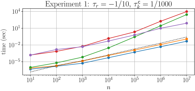
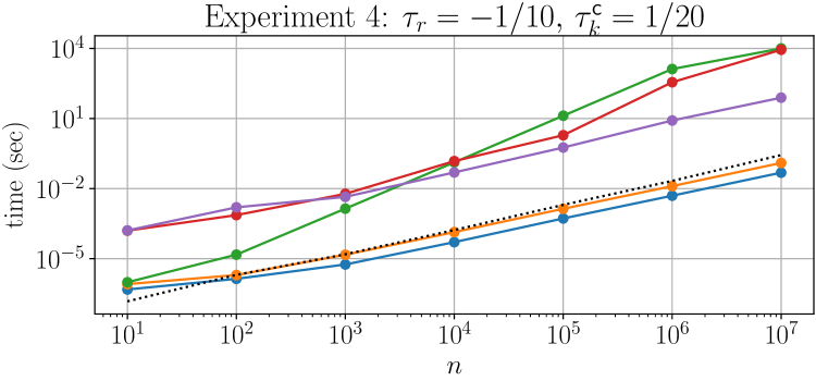
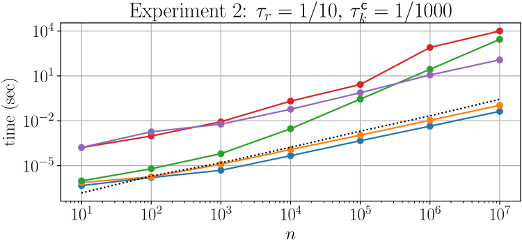
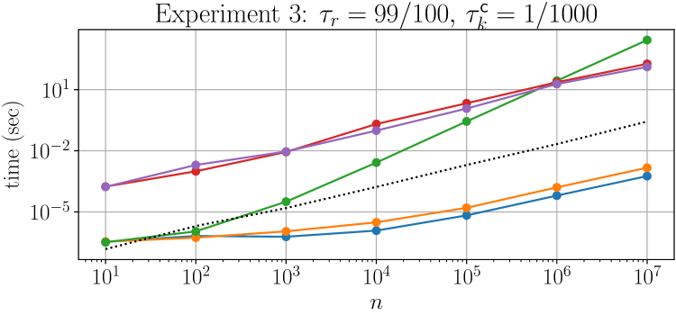
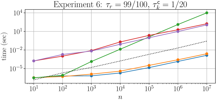
Figure 4: Average total computation time excluding sort time and full sort time vs $n$. All results are averaged over 100 instances, except for methods GRID, GRBS, and GRBU with $n\in\{10^{6},10^{7}\}$ in which a time-limit of $10^{4}$ seconds is imposed across 2 instances.

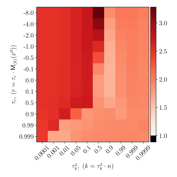
(a) PLCP vs ESGS at $n=10^{7}$.

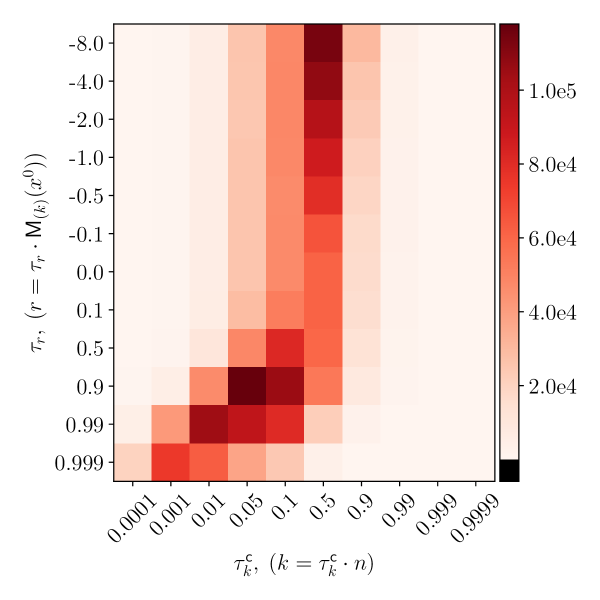
(b) GRID vs ESGS at $n=10^{5}$.

Figure 5: Computation time relative to ESGS averaged over 100 instances. A value of $c>0$ indicates that ESGS was $c$ times faster than the other method; a value of $c<0$ indicates that the other method was $c$ times faster than ESGS. Across all scenarios at $n=10^{5}$, the better of GRBS and GRBU was at best $\approx 350$ times slower than ESGS (and never faster).

	Experiment 1: $\tau_{r}=-1/10,\,\tau_{k}^{\mathsf{c}}=1/1000$
	$n=10^{3}$	$n=10^{4}$	$n=10^{5}$	$n=10^{6}$	$n=10^{7}$
ESGS	5.5e-6 (1e-6)	5.4e-5 (1e-5)	5.3e-4 (10e-5)	4.9e-3 (6e-5)	4.7e-2 (10e-4)
PLCP	1.4e-5 (2e-6)	1.4e-4 (3e-5)	1.2e-3 (2e-4)	1.2e-2 (3e-4)	1.2e-1 (3e-3)
GRID	6.8e-5 (8e-6)	3.0e-3 (2e-4)	2.8e-1 (1e-2)	2.7e+1* (5e-2*)	2.8e+3* (3e0*)
GRBS	5.8e-3 (4e-4)	1.5e-1 (10e-3)	2.2e+0 (2e-1)	1.8e+2* (1e-1*)	9.6e+3* (2e1*)
GRBU	4.9e-3 (3e-4)	5.1e-2 (9e-3)	6.2e-1 (10e-2)	9.9e+0* (8e-2*)	7.9e+1* (1e0*)
	Experiment 2: $\tau_{r}=1/10,\,\tau_{k}^{\mathsf{c}}=1/1000$
	$n=10^{3}$	$n=10^{4}$	$n=10^{5}$	$n=10^{6}$	$n=10^{7}$
ESGS	4.9e-6 (1e-7)	4.7e-5 (8e-6)	4.6e-4 (7e-5)	4.4e-3 (5e-5)	4.3e-2 (6e-4)
PLCP	1.2e-5 (1e-6)	1.2e-4 (2e-5)	1.1e-3 (2e-4)	1.1e-2 (2e-4)	1.1e-1 (2e-3)
GRID	6.3e-5 (5e-6)	2.9e-3 (2e-4)	2.8e-1 (1e-2)	2.7e+1* (6e-2*)	2.8e+3* (4e0*)
GRBS	8.6e-3 (1e-3)	2.1e-1 (1e-2)	2.7e+0 (3e-1)	8.0e+2* (2e0*)	1.0e+4* ($-$*)
GRBU	5.9e-3 (5e-4)	5.9e-2 (7e-3)	7.5e-1 (1e-1)	1.1e+1* (2e-1*)	1.2e+2* (4e0*)
	Experiment 3: $\tau_{r}=99/100,\,\tau_{k}^{\mathsf{c}}=1/1000$
	$n=10^{3}$	$n=10^{4}$	$n=10^{5}$	$n=10^{6}$	$n=10^{7}$
ESGS	6.0e-7 (1e-7)	1.2e-6 (3e-7)	6.7e-6 (1e-6)	6.3e-5 (7e-6)	5.7e-4 (1e-5)
PLCP	1.1e-6 (2e-7)	3.1e-6 (10e-7)	1.6e-5 (3e-6)	1.6e-4 (7e-6)	1.5e-3 (3e-5)
GRID	3.2e-5 (2e-6)	2.6e-3 (5e-4)	2.7e-1 (2e-2)	2.7e+1* (7e-2*)	2.7e+3* (4e0*)
GRBS	8.7e-3 (6e-4)	2.1e-1 (1e-2)	2.1e+0 (2e-1)	2.3e+1* (4e-1*)	1.8e+2* (3e-1*)
GRBU	9.2e-3 (4e-4)	9.8e-2 (1e-2)	1.2e+0 (1e-1)	1.9e+1* (7e-1*)	1.3e+2* (2e-1*)
	Experiment 4: $\tau_{r}=-1/10,\,\tau_{k}^{\mathsf{c}}=1/20$
	$n=10^{3}$	$n=10^{4}$	$n=10^{5}$	$n=10^{6}$	$n=10^{7}$
ESGS	5.6e-6 (1e-6)	5.1e-5 (3e-6)	5.3e-4 (9e-5)	5.0e-3 (5e-5)	4.8e-2 (4e-4)
PLCP	1.5e-5 (2e-6)	1.4e-4 (10e-6)	1.4e-3 (2e-4)	1.3e-2 (2e-4)	1.3e-1 (2e-3)
GRID	1.4e-3 (9e-5)	1.3e-1 (2e-3)	1.3e+1 (1e-1)	1.3e+3* (2e0*)	1.0e+4* ($-$*)
GRBS	6.0e-3 (3e-4)	1.5e-1 (9e-3)	1.9e+0 (2e-1)	3.6e+2* (3e0*)	8.8e+3* (2e0*)
GRBU	4.4e-3 (2e-4)	4.9e-2 (8e-3)	5.7e-1 (7e-2)	8.2e+0* (1e-1*)	7.8e+1* (6e0*)
	Experiment 5: $\tau_{r}=1/10,\,\tau_{k}^{\mathsf{c}}=1/20$
	$n=10^{3}$	$n=10^{4}$	$n=10^{5}$	$n=10^{6}$	$n=10^{7}$
ESGS	5.2e-6 (7e-7)	4.6e-5 (2e-6)	4.6e-4 (7e-6)	4.5e-3 (5e-5)	4.4e-2 (4e-4)
PLCP	1.4e-5 (3e-6)	1.2e-4 (4e-6)	1.2e-3 (2e-5)	1.2e-2 (2e-4)	1.1e-1 (2e-3)
GRID	1.4e-3 (8e-5)	1.3e-1 (2e-3)	1.3e+1 (1e-1)	1.3e+3* (2e0*)	1.0e+4* ($-$*)
GRBS	8.2e-3 (7e-4)	2.0e-1 (1e-2)	2.4e+0 (2e-1)	3.1e+3* (2e1*)	1.0e+4* ($-$*)
GRBU	5.3e-3 (3e-4)	5.7e-2 (5e-3)	6.7e-1 (5e-2)	9.8e+0* (2e0*)	9.8e+1* (4e0*)
	Experiment 6: $\tau_{r}=99/100,\,\tau_{k}^{\mathsf{c}}=1/20$
	$n=10^{3}$	$n=10^{4}$	$n=10^{5}$	$n=10^{6}$	$n=10^{7}$
ESGS	6.7e-7 (2e-7)	1.9e-6 (2e-7)	1.4e-5 (3e-6)	1.4e-4 (3e-6)	1.4e-3 (2e-5)
PLCP	1.3e-6 (2e-7)	3.8e-6 (1e-6)	3.3e-5 (4e-6)	2.7e-4 (6e-6)	2.5e-3 (5e-5)
GRID	1.4e-4 (5e-5)	1.3e-2 (2e-3)	1.3e+0 (6e-2)	1.3e+2* (2e0*)	1.0e+4* ($-$*)
GRBS	8.0e-3 (5e-4)	2.0e-1 (2e-2)	2.3e+0 (3e-1)	1.9e+1* (2e-1*)	1.7e+2* (4e0*)
GRBU	6.8e-3 (3e-4)	8.5e-2 (2e-2)	9.5e-1 (7e-2)	9.7e+0* (2e0*)	1.1e+2* (4e0*)
Sort time (full)	1.5e-5	1.7e-4	2.0e-3	2.1e-2	2.7e-1
Sort time (top-1%)	8.0e-6	7.2e-5	7.4e-4	7.0e-3	7.3e-2

Table 1: Mean computation time and (standard deviation) in seconds for projecting an initial sorted vector $x^{0}$ drawn uniformly from $[0,1]^{n}$ onto $\mathcal{B}^{r}_{(k)}$ with $r=\tau_{r}\cdot\mathds{1}_{k}^{\top}x^{0}$ and $k=\tau_{k}^{\mathsf{c}}\cdot n$. Statistics are computed over 100 ($2^{*}$) instances, and the fastest method is listed in bold. A dash “$-$” for standard deviation indicates that the experiment timed out in each instance. The full and top-1% sort time is listed for reference and is not counted towards the solve time for any method.

Results and discussion

The numerical results are summarized in Table 1, and Fig. 4 and Fig. 5.

Across all values of $n$, our two proposed methods consistently outperform the existing grid-search method and the Gurobi QP solver, often achieving improvements by several orders of magnitude. The scaling profile in Fig. 4 reveals the linear behavior of our proposed methods and the sparsity-exploiting inexact method GRBU based on the formulation (5). In contrast, the grid-search method exhibits quadratic scaling, and the sorted inexact method GRBS based on (5i) exhibits performance that degrades in harder large-$n$ cases. For problem sizes where $n\in\{10^{6},10^{7}\}$, the solution time of the grid-search and Gurobi methods is on the order of minutes or hours; on the other hand, our methods obtain solutions in fractions of a second.

In Table 1, we highlight the computational results for a few experiments based on parameters which we expect to be of practical interest. In Experiments 1 through 3, we fix $k$ to be a small proportion of $n$ and vary the budget $r$ from large to small; Experiments 4 through 6 follow a similar pattern, but with a larger value of $k$. A clear takeaway from the results is that the (full) sorting procedure requires more time than solution procedure of our proposed algorithms for sorted input. This highlights the importance of Proposition 3. Sorting is also more costly than the grid-search method for small $n$, but for moderate-to-large $n$, the $O(k(n-k))$ computational cost of the grid-search method dominates the sorting time, even for very small $\tau_{k}$ as in Experiments 1 through 3.

Another observation from Table 1 is that the performance of the finite-termination algorithms are problem-dependent, with the grid-search method being the most variable. On the other hand, the performance of the Gurobi QP solver based on the unsorted formulation (5) is relatively stable across different instances, in addition to being significantly more efficient than the sorted formulation (5i). A plausible reason for this phenomenon is that the number of active constraints at the solutions are different for the two formulations: for instances in Experiments 3 and 6 with $n=10^{6}$, the sorted formulation yields averages of $10^{4}$ and $9.6\times 10^{3}$ number of active constraints, compared to $9.8\times 10^{3}$ and $3.8\times 10^{3}$ for the unsorted formulation. Theoretically, only $\lvert\beta\rvert$ number of constraints (see Fig. 1) should be binding for the unsorted formulation, whereas many more constraints could be binding for the sorted formulation.

Fig. 5 compares the relative performance of the proposed methods across the entire spectrum of the parameters $r$ and $k$. Fig. 5(a) shows that ESGS performs about 1.5-2 times better (and never worse) than PLCP across the spectrum, though its advantage degrades in the easier instances in which $\tau_{r}\approx 1$. Fig. 5(b) shows that ESGS performs significantly better than GRID in many cases of practical interest (see the bottom of the “backwards L” in the lower lefthand corner) where we observe excesses of $10^{4}$-fold run-time improvement.

5 Conclusions

We have provided two efficient, finite-termination algorithms, PLCP and ESGS, that are capable of exactly solving the top-$k$-sum projection problem (1). When the input vector is unsorted, the solution requires a complexity of $O(n\log n)$, and when sorted, it reduces to $O(n)$. These implementations improve upon existing methods by orders of magnitude in many cases of interest; notably, they are over 100 times faster than Gurobi and the existing grid-search method. Our numerical experiments also show that ESGS improves upon PLCP by a factor of $\approx 2$ in harder instances where many pivots are required while maintaining a slight advantage in easier instances that require fewer pivots. Such easy instances frequently arise when solving a sequence of similar problems, such as employing an iterative method to solve superquantile constrained optimization problems in the form of (2), which necessitate repeated calls to a projection oracle. Moreover, our proposed techniques, with minimal modifications, can be applied to compute the projection onto the vector-$k$-norm ball. In this case, PLCP can avoid incurring an additional $O(k)$ cost that an ESGS-based approach unavoidably pays (see Step 1 in [wu2014moreau, Algorithm 4]).

6 Algorithmic detail

6.1 PLCP

We recall some background for processing a PLCP($\lambda;q,d,M$) where $q\geq 0_{n-1}$ and $M$ is a symmetric, positive definite $Z$-matrix before specializing to the sorted projection problem (5i). The approach largely follows the symmetric parametric principal pivoting method outlined in [cottle2009lcp, Algorithm 4.5.2], but instead of computing the upper bound for $\lambda$ ahead of time, we check the whether or not the existing solution satisfies the top-$k$-sum budget constraint at each iteration. We begin by noting that any basis $\xi\subseteq\{1,\ldots,n-1\}$ partitions the affine relationship into the following system

$$\begin{bmatrix}w_{\xi}(\lambda)\\ w_{\xi^{\mathsf{c}}}(\lambda)\end{bmatrix}=\begin{bmatrix}M_{\xi\xi}&M_{\xi\xi^{\mathsf{c}}}\\ M_{\xi^{\mathsf{c}}\xi}&M_{\xi^{\mathsf{c}}\xi^{\mathsf{c}}}\end{bmatrix}\begin{bmatrix}z_{\xi}(\lambda)\\ z_{\xi^{\mathsf{c}}}(\lambda)\end{bmatrix}+\begin{bmatrix}q_{\xi}+\lambda d_{\xi}\\ q_{\xi^{\mathsf{c}}}+\lambda d_{\xi^{\mathsf{c}}}\end{bmatrix},$$ (5afcf)

where the notation $w(\lambda)$ and $z(\lambda)$ is used to emphasize the dependence on parameter $\lambda$, and where the linear system always has a unique solution for every $\xi$ since $M$ has positive principal minors. The PLCP solves the projection problem (5i) by identifying an optimal basis $\bar{\xi}$ and parameter $\bar{\lambda}\geq 0$ such that the solution ${w}(\bar{\lambda})$ and ${z}(\bar{\lambda})$ satisfy:

• subproblem optimality for LCP($q+\bar{\lambda}d,M$): this consists of (i) complementarity: ${w}_{\bar{\xi}}(\bar{\lambda})=0$ and ${z}_{\bar{\xi}^{\mathsf{c}}}(\bar{\lambda})=0$; and (ii) feasibility: ${z}_{\bar{\xi}}(\bar{\lambda})\geq 0$, ${w}_{\bar{\xi}^{\mathsf{c}}}(\bar{\lambda})\geq 0$, and ${w}(\bar{\lambda})=M{z}(\bar{\lambda})+q+\bar{\lambda}d$;

• outer problem optimality: the primal solution $\bar{x}(\bar{\lambda})=\reflectbox{$\vec{\reflectbox{$x$}}$}^{0}-\bar{\lambda}\mathds{1}_{k}+D^{\top}\bar{z}$, which is an implicit function of $\lambda$, satisfies $\mathds{1}_{k}^{\top}{x}(\bar{\lambda})=r$, assuming that $\mathds{1}_{k}^{\top}\reflectbox{$\vec{\reflectbox{$x$}}$}^{0}>r$.

Under the present setting, the parametric LCP procedure begins by solving the trivial LCP$(q,M)$ associated with $\lambda=0$ by taking $\xi=\emptyset$, $z\equiv 0$, and $w=q\geq 0$. This solution, denoted $\bigl{(}z(0),w(0)\bigr{)}$ may not satisfy the budget constraint, in which case $\lambda$ needs to be increased. The remaining steps utilize the fact that the solution map $z(\lambda)$ associated with the LCP subproblem at value $\lambda$ is a piecewise-linear and monotone nondecreasing function in $\lambda$. Therefore, as $\lambda$ increases, the procedure only “adds” nonnegative components to $z(\lambda)$. It stops once a large enough $\lambda\geq 0$ has been identified so that the budget constraint is satisfied.

The mechanics of the PLCP specialized to our problem are as follows. To solve any LCP subproblem associated with $\lambda$, we seek identify a complementary, feasible basis $\xi$ (depending on $\lambda$) of dimension $m$ that gives rise to the solution map

$$z_{\xi}(\lambda) =M_{\xi\xi}^{-1}(-q_{\xi}-\lambda d_{\xi})=z_{\xi}(0)-\lambda M_{\xi\xi}^{-1}d_{\xi}$$ (5afcga)

$$w_{\xi^{\mathsf{c}}}(\lambda) =M_{\xi^{\mathsf{c}}\xi}z_{\xi}+q_{\xi^{\mathsf{c}}}+\lambda d_{\xi^{\mathsf{c}}}$$ (5afcgb)

via the linear system (5afcf) where $M_{\xi\xi}^{-1}\coloneqq(M_{\xi\xi})^{-1}$.

We will show three things: (i) beginning from $\xi^{1}=\{k\}$ in iteration 1, $\xi^{t}$ remains contiguous for all subsequent iterations $t\geq 1$, which leads to a simple form of the minimum ratio test for identifying the breakpoint $\lambda^{t+1}$ and indicates that a basis $\xi^{t}$ is subproblem-optimal for $\lambda\in[\lambda^{t},\lambda^{t+1}]$; (ii) checking whether or not $\lambda^{t+1}$ is “large enough” simplifies, i.e., that there exists $\bar{\lambda}\leq\lambda^{t+1}$ such that the primal solution ${x}(\bar{\lambda})$ satisfies the budget constraint; and (iii) updating the solution map $z(\lambda^{t+1})$ associated with the new breakpoint $\lambda^{t+1}$ from the previous solution $z(\lambda^{t})$ simplifies. In the below subsections, we drop the dependence on $t$ and use “$+$” to denote the next value when clear. The simplified expressions for each step involve the observation that $M_{\xi\xi}^{-1}$ has an explicit form given by

$$(M_{\xi\xi})^{-1}_{ij}=\frac{(\lvert\xi\rvert+1-\max(i,j))\cdot\min(i,j)}{\lvert\xi\rvert+1}.$$ (5afch)

Identifying the next breakpoint

Suppose that $w(\lambda)\geq 0$ and $z(\lambda)\geq 0$ are optimal for the subproblem with parameter $\lambda$ and contiguous basis $\xi$ (i.e., $\xi=\{a,a+1,\ldots,b-1,b\}$ for $n-1\geq b\geq a\geq 1$) that contains $k$ with $\lvert\xi\rvert=m$. Inspecting (5afcga), notice that $z_{\xi}(\lambda)=(\leq 0)_{\xi}+\lambda M_{\xi\xi}^{-1}e_{\xi}^{k}$ because $q\geq 0$, $d=-e^{k}$, and because of the fact that $M$ is a $Z$-matrix implies that $M^{-1}_{ij}\geq 0$. Since $M_{\xi\xi}$ also is a $Z$-matrix, it holds that $M_{\xi\xi}^{-1}\geq 0$ and thus that $z_{\xi}(\lambda^{\prime})\geq z_{\xi}(\lambda)$ for $\lambda^{\prime}\geq\lambda$. On the other hand, suppose that the current solution does not satisfy the budget constraint, i.e., $\lambda$ is not large enough. Because of the form of $M=DD^{\top}$, $M_{\xi^{\mathsf{c}}\xi}$ is the matrix of zeros except for at most two negative elements in different columns. Explicitly, the two elements of $M_{\xi^{\mathsf{c}}\xi}z_{\xi}(\lambda)$ are: $-z_{\xi_{1}}(\lambda)$ in index $\xi_{1}-1$ and $-z_{\xi_{m}}(\lambda)$ in index $\xi_{m}+1$. Since $d=-e^{k}$, we may neglect the term $d_{\xi^{\mathsf{c}}}=0$, so there are only two possible indices where $w_{\xi^{\mathsf{c}}}(\lambda)$ may fail to be nonnegative: $a-1$ where $a\coloneqq\xi_{1}$, and $b+1$ where $b\coloneqq\xi_{m}$. As a result, the “minimum ratio test” only requires two comparisons per pivot where the smallest parameter such that $w_{i^{*}}(\lambda)=0$ for some $i^{*}\in\xi^{\mathsf{c}}$ is given by

$$\lambda^{+} \coloneqq\operatorname*{arg\,min}_{\lambda^{\prime}\geq\lambda}\bigl{\{}M_{\xi^{\mathsf{c}}\xi}z_{\xi}(\lambda^{\prime})+q_{\xi^{\mathsf{c}}}=0\bigr{\}}=\operatorname*{arg\,min}_{\lambda^{\prime}\geq\lambda}\bigl{\{}0=-z_{a}(\lambda)+q_{a-1}\;,\;0=-z_{b}(\lambda)+q_{b+1}\bigr{\}}$$

$$=\operatorname*{arg\,min}_{\lambda^{\prime}\geq\lambda}\bigl{\{}0=-z_{a}(0)-\lambda(M_{\xi\xi}^{-1}e^{k}_{\xi})_{\prescript{}{a}{\xi}}+q_{a-1}\;,\;0=-z_{b}(0)-\lambda(M_{\xi\xi}^{-1}e^{k}_{\xi})_{\prescript{}{b}{\xi}}+q_{b+1}\bigr{\}}$$

$$=\min\bigl{\{}{\bigl{(}q_{a-1}-z_{a}(0)\bigr{)}}/(M_{\xi\xi}^{-1}e_{\xi}^{k})_{1}\;,\;{\bigl{(}q_{b+1}-z_{b}(0)\bigr{)}}/(M_{\xi\xi}^{-1}e_{\xi}^{k})_{m}\bigr{\}}=\min\bigl{\{}\lambda^{a},\lambda^{b}\bigr{\}}.$$ (5afci)

The constant cost of determining $\lambda^{+}$ is clear from the explicit expression for $(M_{\xi\xi}^{-1})_{ij}$ via (5afch). If $\lambda^{+}=\lambda^{a}$, then we define $s\coloneqq a-1$ and update the basis $\xi^{+}=(s,\xi)$; otherwise we define $s\coloneqq b+1$ and set $\xi^{+}=(\xi,s)$. Therefore, the next basis $\xi^{+}$ is contiguous and contains $k$. Next we must check whether $\lambda^{+}\geq\bar{\lambda}$, i.e., whether the current basis contains a solution that satisfies the budget constraint for some parameter in the range $[\lambda,\lambda^{+}]$.

Checking optimality

The procedure terminates based on the observation that for the next breakpoint $\lambda^{+}$ (as determined above with current basis $\xi$), if $\mathsf{T}_{(k)}(x(\lambda^{+}))<r$ with current basis $\xi$, then there must exist a $\bar{\lambda}<\lambda^{+}$ that solves $\mathsf{T}_{(k)}(x(\bar{\lambda}))=r$ for basis $\xi$. From the primal solution map ${x}(\lambda)=\reflectbox{$\vec{\reflectbox{$x$}}$}^{0}-\lambda\mathds{1}_{k}+D^{\top}z(\lambda)$, which is derived from stationarity of the Lagrangian, evaluation of the top-$k$-sum simplifies to $\mathsf{T}_{(k)}(x(\lambda))=\mathds{1}_{k}^{\top}{x}(\lambda)=\sum_{i=1}^{k}\reflectbox{$\vec{\reflectbox{$x$}}$}_{i}^{0}-k\lambda+z_{k}(\lambda)$ where

$$z_{k}(\lambda) =-(M_{\xi\xi}^{-1}q_{\xi})_{\prescript{}{k}{\xi}}+\lambda\cdot(M_{\xi\xi}^{-1}e^{k}_{\xi})_{\prescript{}{k}{\xi}}=z_{k}(0)+\lambda\cdot(M_{\xi\xi}^{-1}e^{k}_{\xi})_{\prescript{}{k}{\xi}}.$$

If $\mathsf{T}_{(k)}({x}(\lambda^{+}))<r$, then $\bar{\lambda}$ satisfies

$$\bar{\lambda}=\Bigl{(}\sum_{i=1}^{k}\reflectbox{$\vec{\reflectbox{$x$}}$}^{0}_{i}-r+z_{k}(0)\Bigr{)}/\bigl{(}k-(M_{\xi\xi}^{-1})_{\prescript{}{k}{\xi}\prescript{}{k}{\xi}}\bigr{)},$$ (5afcj)

which can be done in constant time due to (5afch). Finally, we can reconstruct $\bar{x}(\bar{\lambda})=\reflectbox{$\vec{\reflectbox{$x$}}$}^{0}-\bar{\lambda}\mathds{1}_{k}+D^{\top}z(\bar{\lambda})$. Since $D$ has only two elements per row, and by observing that $z_{\xi^{\mathsf{c}}}(\bar{\lambda})=0$, the matrix-vector multiplication can be performed in $O(\lvert\xi\rvert)$ time. Otherwise, it remains to update the solution maps $z_{\xi^{+}}(\lambda^{+})$ and $w_{\xi^{+}}(\lambda^{+})$ and then return to the breakpoint identification step.

Updating the subproblem solution

Thus far, excluding the recovery of a primal optimal solution, our procedure has required computations involving only a very particular subset of $z_{\xi}(0)$, namely $z_{a}(0)$, $z_{k}(0)$, and $z_{b}(0)$. This observation allows for performing a constant number of updates per iteration. Since $\xi^{+}\setminus\xi=\{s\}$ changes by one element per iteration and $\xi^{+}$ remains contiguous, the Schur complement rule can be used to update the three elements of $z_{\xi^{+}}(0)$ in constant time, which in turn provides the new solution via $z_{\xi^{+}}(\lambda^{+})=z_{\xi^{+}}(0)+\lambda M_{\xi^{+}\xi^{+}}^{-1}e^{k}$, where the latter term can be computed in constant time from the form of $M^{-1}$ given by (5afch).

Accordingly, the goal of this section is to compute $z_{\xi^{+}_{a^{+}}}(0)$, $z_{\xi^{+}_{k^{+}}}(0)$, and $z_{\xi^{+}_{b^{+}}}(0)$ for basis $\xi^{+}$ at (new) locations $a^{+}$, $k^{+}$, and $b^{+}$ in $\xi^{+}$ from an existing solution $z_{\xi{a}}(0)$, $z_{\xi_{k}}(0)$, and $z_{\xi_{b}}(0)$ with basis $\xi$. There are two cases, corresponding to $\xi^{+}=\xi\cup\{s\}$ with

1. $s=a-1$. Then $\xi^{+}=(a-1,\xi)$ so that $a^{+}=a-1$, and

   $$z_{\xi^{+}}(0) =\begin{bmatrix}z_{s}(0)\\ z_{\xi}(0)\end{bmatrix}=-M_{\xi^{+}\xi^{+}}^{-1}q_{\xi^{+}}=\begin{bmatrix}2&(-1,0,\ldots,0)\\ (-1,0,\ldots,0)^{\top}&M_{\xi\xi}\end{bmatrix}^{-1}\begin{bmatrix}-q_{s}\\ -q_{\xi}\end{bmatrix}$$

   $$=\begin{bmatrix}\tfrac{1}{\sigma}(z_{a}(0)-q_{a-1}\\ z_{\xi}(0)+\tfrac{1}{\sigma}(M_{\xi\xi}^{-1})_{\xi,1}\cdot(z_{a}(0)-q_{a-1}\end{bmatrix},$$

   where $t_{a}=(-1,0,\ldots,0)^{\top}$ and $\sigma=2-t_{a}^{\top}M_{\xi\xi}^{-1}t_{a}=2-(M_{\xi\xi}^{-1})_{1,1}=(m+2)/(m+1)$. Thus

   $$a^{+} =a-1,\quad\prescript{}{a^{+}}{\xi^{+}}=1,\quad\prescript{}{k^{+}}{\xi^{+}}=\prescript{}{k}{\xi}+1,\quad\prescript{}{b^{+}}{\xi^{+}}=\prescript{}{b}{\xi}+1$$

   $$z_{{a^{+}}}(0) =\tfrac{1}{\sigma}(z_{a}(0)-q_{a-1}(0))$$

   $$z_{{k^{+}}}(0) =z_{k}(0)+(M_{\xi\xi}^{-1})_{\prescript{}{k}{\xi},1}\cdot\tfrac{1}{\sigma}(z_{a}(0)-q_{a-1}(0))=z_{k}(0)+(M_{\xi\xi}^{-1})_{\prescript{}{k}{\xi},1}\cdot z_{{a^{+}}}(0)$$

   $$z_{{b^{+}}}(0) =z_{b}(0)+(M_{\xi\xi}^{-1})_{m,1}\cdot\tfrac{1}{\sigma}(z_{a}(0)-q_{a-1}(0))=z_{b}(0)+(M_{\xi\xi}^{-1})_{\xi_{b},\xi_{a}}\cdot z_{{a^{+}}}(0).$$

2. $s=b+1$. Then $\xi^{+}=(\xi,b+1)$ so that $b^{+}=b+1$, and

   $$z_{\xi^{+}}(0) =\begin{bmatrix}z_{\xi}(0)\\ z_{s}(0)\end{bmatrix}=-M_{\xi^{+}\xi^{+}}^{-1}q_{\xi^{+}}=\begin{bmatrix}M_{\xi\xi}&(0,\ldots,0,-1)^{\top}\\ (0,\ldots,0,-1)&2\end{bmatrix}^{-1}\begin{bmatrix}-q_{\xi}\\ -q_{s}\end{bmatrix}$$

   $$=\begin{bmatrix}z_{\xi}(0)+\tfrac{1}{\sigma}(M_{\xi\xi}^{-1})_{\xi,m}\cdot(z_{b}(0)-q_{b+1}\\ \tfrac{1}{\sigma}(z_{b}(0)-q_{b+1}\end{bmatrix},$$

   where $t_{b}=(0,\ldots,0,-1)^{\top}$ and $\sigma=2-t_{b}^{\top}(M_{\xi\xi}^{-1})t_{b}=2-(M_{\xi\xi}^{-1})_{m,m}=(m+2)/(m+1)$. Thus

   $$b^{+} =b+1,\quad\prescript{}{a^{+}}{\xi^{+}}=1,\quad\prescript{}{k^{+}}{\xi^{+}}=\prescript{}{k}{\xi},\quad\prescript{}{b^{+}}{\xi^{+}}=\prescript{}{b}{\xi}+1$$

   $$z_{{a^{+}}}(0) =z_{{a}}(0)+(M_{\xi\xi}^{-1})_{1,m}\cdot\tfrac{1}{\sigma}(z_{b}(0)-q_{b+1})=z_{{a}}(0)+(M_{\xi\xi}^{-1})_{1,m}\cdot z_{{b^{+}}}(0)$$

   $$z_{{k^{+}}}(0) =z_{{k}}(0)+(M_{\xi\xi}^{-1})_{\prescript{}{k}{\xi},m}\cdot\tfrac{1}{\sigma}(z_{b}(0)-q_{b+1})=z_{{k}}(0)+(M_{\xi\xi}^{-1})_{\prescript{}{k}{\xi},m}\cdot z_{{b^{+}}}(0)$$

   $$z_{{b^{+}}}(0) =\tfrac{1}{\sigma}\cdot(z_{b}(0)-q_{b+1}).$$

The constant cost of the solution update procedure is clear due to the explicit formula for $(M_{\xi\xi}^{-1})_{ij}$.

Recovering $k_{0}$ and $k_{1}$

Given optimal indices $\bar{a}$ and $\bar{b}$ and a solution $\bar{x}$ produced by PLCP, the sorting-indices $k_{0}$ and $k_{1}$ can be recovered without inspecting $\bar{x}$ by setting $(\bar{k}_{0},\bar{k}_{1})=(k-1,k)$ if the problem is solved immediately; otherwise $(\bar{k}_{0},\bar{k}_{1})=\bigl{(}\max\{\bar{a}-1,0\},\min\{\bar{b}+1,n\}\bigr{)}$.

6.2 ESGS

We now provide additional details justifying the form of (i) the candidate solution for a given candidate index-pair $(k_{0}^{\prime},k_{1}^{\prime})$ in (5ad); and (ii) the form of the KKT conditions (5ae) that are used in the analysis of the ESGS algorithm.

Candidate solution

We now provide an argument justifying the construction of the linear system in $\theta^{\prime},\lambda^{\prime}$ and candidate solution $x^{\prime}(k_{0}^{\prime},k_{1}^{\prime})$ from (5ad). The linear equations in $\lambda^{\prime}$ and $\theta^{\prime}$ are recovered by summing various components of the KKT conditions

$$k_{0}^{\prime}\lambda^{\prime}=\sum_{i=1}^{k_{0}^{\prime}}x_{i}^{0}-r+\theta^{\prime}(k-k_{0}^{\prime}),\quad\text{and}\quad(k_{1}^{\prime}-k_{0}^{\prime})\theta^{\prime}=\sum_{i=k_{0}^{\prime}+1}^{k_{1}^{\prime}}x_{i}^{0}-\lambda^{\prime}(k-k_{0}^{\prime}).$$ (5afck)

The equation for $\lambda^{\prime}$ is recovered by summing the stationarity conditions corresponding to indices in $\alpha^{\prime}$ and eliminating $\mathds{1}_{\alpha^{\prime}}^{\top}{x}^{\prime}_{\alpha^{\prime}}$ using the constraint. That is, $\sum_{i=1}^{k_{0}^{\prime}}x_{i}^{\prime}=\sum_{i=1}^{k_{0}^{\prime}}(\reflectbox{$\vec{\reflectbox{$x$}}$}_{i}^{0}-\lambda^{\prime})$ and $r=\sum_{i=1}^{k_{0}^{\prime}}x^{\prime}_{i}+(k-k_{0}^{\prime})\theta^{\prime}$ imply $\sum_{i=1}^{k_{0}^{\prime}}\reflectbox{$\vec{\reflectbox{$x$}}$}_{i}^{0}-k_{0}^{\prime}\lambda^{\prime}=r-(k-k_{0}^{\prime})\theta^{\prime}$. On the other hand, equation $\theta^{\prime}$ is recovered by summing the stationarity conditions corresponding to indices in $\beta^{\prime}$ and using $\mathds{1}_{\beta^{\prime}}^{\top}\mu^{\prime}=(k-k_{0})$. That is, $\sum_{i=k_{0}^{\prime}+1}^{k_{1}^{\prime}}x_{i}^{\prime}=\sum_{i=k_{0}^{\prime}+1}^{k_{1}^{\prime}}\reflectbox{$\vec{\reflectbox{$x$}}$}_{i}^{0}-(k-k_{0}^{\prime})\lambda^{\prime}$ and $\sum_{i=k_{0}^{\prime}+1}^{k_{1}^{\prime}}x_{i}^{\prime}=(k_{1}^{\prime}-k_{0}^{\prime})\theta^{\prime}$. The linear system $A\cdot(\lambda,\theta)^{\top}=b$ has explicit solution

$$A \coloneqq\begin{bmatrix}k_{0}&-(k-k_{0})\\ k-k_{0}&k_{1}-k_{0}\end{bmatrix},\quad b\coloneqq\begin{bmatrix}\sum_{i=1}^{k_{0}}\reflectbox{$\vec{\reflectbox{$x$}}$}_{i}^{0}-r\\ \sum_{i=k_{0}+1}^{k_{1}}\reflectbox{$\vec{\reflectbox{$x$}}$}_{i}^{0}\end{bmatrix},\quad A^{-1}=\frac{1}{\rho}\begin{bmatrix}k_{1}-k_{0}&k-k_{0}\\ -(k-k_{0})&k_{0}\end{bmatrix},$$

where $\rho\coloneqq\operatorname{\mathsf{det}}[A]=k_{0}(k_{1}-k_{0})+(k-k_{0})^{2}$.

KKT conditions

Next we justify the reduction of the KKT conditions from (5ac) to the five conditions listed in (5ae). The KKT conditions (5ac) are equivalent to (5ae) because of the following argument. Inspecting condition $\bar{x}_{\bar{k}_{0}}>\bar{\theta}$ at index $k_{0}^{\prime}$ and using $\bar{x}_{\bar{\beta}}=\bar{\theta}_{\bar{\beta}}$ to obtain $x_{k_{0}^{\prime}+1}^{\prime}=\theta^{\prime}$, it holds that

$$\begin{cases}x_{k_{0}^{\prime}}^{\prime}>\theta^{\prime}\iff\reflectbox{$\vec{\reflectbox{$x$}}$}_{k_{0}^{\prime}}^{0}-\lambda^{\prime}>\theta^{\prime}\iff\reflectbox{$\vec{\reflectbox{$x$}}$}_{k_{0}^{\prime}}^{0}>\theta^{\prime}+\lambda^{\prime}\\ \theta^{\prime}+\lambda^{\prime}=x_{k_{0}^{\prime}+1}^{\prime}+\lambda^{\prime}=\reflectbox{$\vec{\reflectbox{$x$}}$}_{k_{0}^{\prime}+1}^{0}-\lambda^{\prime}\mu_{k_{0}^{\prime}+1}^{\prime}+\lambda^{\prime}\overset{(*)}{\geq}\reflectbox{$\vec{\reflectbox{$x$}}$}_{k_{0}^{\prime}+1}^{0}\end{cases}\iff\quad\reflectbox{$\vec{\reflectbox{$x$}}$}_{k_{0}^{\prime}}^{0}>\theta^{\prime}+\lambda^{\prime}\geq\reflectbox{$\vec{\reflectbox{$x$}}$}_{k_{0}^{\prime}+1}^{0},$$

where $(*)$ holds since $\mu^{\prime}_{k_{0}^{\prime}+1}\in[0,1]$ and $\lambda^{\prime}>0$. Similarly, inspecting condition $\bar{\theta}\geq\bar{x}_{\bar{k}_{1}+1}$ at index $k_{1}^{\prime}$ and using $\bar{x}_{\bar{\beta}}=\bar{\theta}\mathds{1}_{\bar{\beta}}$ to obtain $x_{k_{1}^{\prime}}^{\prime}=\theta^{\prime}$, it holds that

$$\begin{cases}\theta^{\prime}>x_{k_{1}^{\prime}+1}^{\prime}=\reflectbox{$\vec{\reflectbox{$x$}}$}_{k_{1}^{\prime}+1}^{0}\\ \theta^{\prime}=x_{k_{1}^{\prime}}^{\prime}=\reflectbox{$\vec{\reflectbox{$x$}}$}_{k_{1}^{\prime}}^{0}-\mu_{k_{1}^{\prime}+1}^{\prime}\lambda^{\prime}\overset{(**)}{\leq}x_{k_{1}^{\prime}}^{0}\end{cases}\iff\quad\reflectbox{$\vec{\reflectbox{$x$}}$}_{k_{1}^{\prime}}^{0}\geq\theta^{\prime}>\reflectbox{$\vec{\reflectbox{$x$}}$}_{k_{1}^{\prime}+1}^{0},$$

where $(**)$ holds since $\mu^{\prime}_{k_{1}^{\prime}}\in[0,1]$ and $\lambda^{\prime}>0$.

References

• [1] Philippe Artzner, Freddy Delbaen, Jean-Marc Eber, and David Heath. Coherent measures of risk. Mathematical Finance, 9(3):203–228, December 1999.
• [2] Francis Bach. Learning with submodular functions: A convex optimization perspective. Foundations and Trends in Machine Learning, 6(2-3):145–373, November 2013.
• [3] Richard. E. Barlow and Hugh. D. Brunk. The isotonic regression problem and its dual. Journal of the American Statistical Association, 67(337):140–147, March 1972.
• [4] Michael J. Best and Nilotpal Chakravarti. Active set algorithms for isotonic regression; a unifying framework. Mathematical Programming, 47(1):425–439, May 1990.
• [5] Jeff Bezanson, Alan Edelman, Stefan Karpinski, and Viral B. Shah. Julia: A fresh approach to numerical computing. SIAM Review, 59(1):65–98, 2017.
• [6] Ramaswamy Chandrasekaran. A special case of the complementary pivot problem. Opsearch, 7:263–268, 1970.
• [7] Anirban Chaudhuri, Boris Kramer, Matthew Norton, Johannes O. Royset, and Karen Willcox. Certifiable risk-based engineering design optimization. American Institute of Aeronautics and Astronautics Journal, 60(2):551–565, February 2022.
• [8] Wenqing Chen, Melvyn Sim, Jie Sun, and Chung-Piaw Teo. From CVaR to uncertainty set: Implications in joint chance-constrained optimization. Operations Research, 58(2):470–485, October 2010.
• [9] Richard W. Cottle. Monotone solutions of the parametric linear complementarity problem. Mathematical Programming, 3(1):210–224, December 1972.
• [10] Richard W. Cottle, Jong-Shi Pang, and Richard E. Stone. The Linear Complementarity Problem. SIAM, October 2009.
• [11] David Tena Cucala, Bernardo Cuenca Grau, Boris Motik, and Egor V. Kostylev. On the correspondence between monotonic max-sum GNNs and datalog, May 2023. https://arxiv.org/abs/2305.18015.
• [12] Robert Dahlgren, Chen-Ching Liu, and Jacques Lawarrée. Risk assessment in energy trading. IEEE Transactions on Power Systems, 18(2):503–511, May 2003.
• [13] Amirhossein Dolatabadi and Behnam Mohammadi-Ivatloo. Stochastic risk-constrained scheduling of smart energy hub in the presence of wind power and demand response. Applied Thermal Engineering, 123:40–49, August 2017.
• [14] Henry Eigen and Amir Sadovnik. TopKConv: Increased adversarial robustness through deeper interpretability. In 20th IEEE International Conference on Machine Learning and Applications (ICMLA), pages 15–22, December 2021.
• [15] Christian Fröhlich and Robert C. Williamson. Risk measures and upper probabilities: Coherence and stratification, June 2022. https://arxiv.org/abs/2206.03183.
• [16] Osman Güler. Generalized linear complementarity problems. Mathematics of Operations Research, 20(2):441–448, May 1995.
• [17] Shu Hu, Xin Wang, and Siwei Lyu. Rank-based decomposable losses in machine learning: A survey. IEEE Transactions on Pattern Analysis and Machine Intelligence, PP, July 2023.
• [18] George Isac and Alexandru B. Németh. Monotonicity of metric projections onto positive cones of ordered euclidean spaces. Archiv der Mathematik, 46(6):568–576, June 1986.
• [19] Rabih A. Jabr. Distributionally robust CVaR constraints for power flow optimization. IEEE Transactions on Power Systems, 35(5):3764–3773, September 2020.
• [20] Yassine Laguel, Krishna Pillutla, Jerome Malick, and Zaid Harchaoui. Superquantiles at work: Machine learning applications and efficient subgradient computation. Set-Valued and Variational Analysis, 29:967–996, December 2021.
• [21] Liu Leqi, Adarsh Prasad, and Pradeep K. Ravikumar. On human-aligned risk minimization. In Advances in Neural Information Processing Systems, volume 32, pages 15029–15038, December 2019.
• [22] Alexandru B. Németh and Soltán Z. Németh. Isotonicity of the projection onto the monotone cone, January 2012. https://arxiv.org/abs/1201.4677.
• [23] Arkadi Nemirovski and Alexander Shapiro. Convex approximations of chance constrained programs. SIAM Journal on Optimization, 17(4):969–996, November 2006.
• [24] Michael L. Overton and Robert. S. Womersley. Optimality conditions and duality theory for minimizing sums of the largest eigenvalues of symmetric matrices. Mathematical Programming, 62(1):321–357, February 1993.
• [25] Konstantin Pavlikov and Stan Uryasev. CVaR norm and applications in optimization. Optimization Letters, 8(7):1999–2020, October 2014.
• [26] Le Peng, Yash Travadi, Rui Zhang, Ying Cui, and Ju Sun. Imbalanced classification in medical imaging via regrouping, October 2022. https://arxiv.org/abs/2210.12234.
• [27] Alexander Robey, Luiz Chamon, George J. Pappas, and Hamed Hassani. Probabilistically robust learning: Balancing average and worst-case performance. In Proceedings of the 39th International Conference on Machine Learning, volume 162, pages 18667–18686. PMLR, July 2022.
• [28] Tyrrell Rockafellar and Stan Uryasev. Optimization of conditional value-at-risk. Journal of Risk, 2(3):21–41, April 1999.
• [29] Johannes O. Royset. Risk-adaptive approaches to learning and decision making: A survey, December 2022. https://arxiv.org/abs/2212.00856.
• [30] Mehdi Tavakoli, Fatemeh Shokridehaki, Mudathir Funsho Akorede, Mousa Marzband, Ionel Vechiu, and Edris Pouresmaeil. CVaR-based energy management scheme for optimal resilience and operational cost in commercial building microgrids. International Journal of Electrical Power and Energy Systems, 100:1–9, September 2018.
• [31] Michael J. Todd. On max-k-sums. Mathematical Programming, 171(1-2):489–517, September 2018.
• [32] Robert Williamson and Aditya Menon. Fairness risk measures. In Proceedings of the 36th International Conference on Machine Learning, volume 97, pages 6786–6797. PMLR, June 2019.
• [33] Bin Wu, Chao Ding, Defeng Sun, and Kim-Chuan Toh. On the Moreau–Yosida regularization of the vector $k$-norm related functions. SIAM Journal on Optimization, 24(2):766–794, January 2014.
• [34] Peipei Yuan, Xinge You, Hong Chen, Qinmu Peng, Yue Zhao, Zhou Xu, Xiao-Yuan Jing, and Zhenyu He. Group sparse additive machine with average top-k loss. Neurocomputing, 395:1–14, June 2020.
\nosectionappendix
{toappendix}