Bridging the Gap between Newton-Raphson Method
and Regularized Policy Iteration

Abstract

Regularization is one of the most important techniques in reinforcement learning algorithms. The well-known soft actor-critic algorithm is a special case of regularized policy iteration where the regularizer is chosen as Shannon entropy. Despite some empirical success of regularized policy iteration, its theoretical underpinnings remain unclear. This paper proves that regularized policy iteration is strictly equivalent to the standard Newton-Raphson method in the condition of smoothing out Bellman equation with strongly convex functions. This equivalence lays the foundation of a unified analysis for both global and local convergence behaviors of regularized policy iteration. We prove that regularized policy iteration has global linear convergence with the rate being $\gamma$ (discount factor). Furthermore, this algorithm converges quadratically once it enters a local region around the optimal value. We also show that a modified version of regularized policy iteration, i.e., with finite-step policy evaluation, is equivalent to inexact Newton method where the Newton iteration formula is solved with truncated iterations. We prove that the associated algorithm achieves an asymptotic linear convergence rate of $\gamma^{M}$ in which $M$ denotes the number of steps carried out in policy evaluation. Our results take a solid step towards a better understanding of the convergence properties of regularized policy iteration algorithms.

I Introduction

Reinforcement learning (RL) [1] has achieved remarkable success in many fields that require sequential decision-making and optimal control, such as games [2], [3], robotics [4], [5] and industrial control [6], [7]. The foundation of RL algorithms lies in the theory of Markov decision process (MDP) [8]. At each time step, the agent chooses an action based on its current state and gets an intermediate reward. The objective is to find an optimal policy that maximizes each state’s value, i.e., the infinite horizon discounted accumulative rewards. The Bellman equation identifies the necessary and sufficient conditions of optimal values based on Bellman’s principle of optimality.

Value iteration and policy iteration are two fundamental algorithms to solve the Bellman equation [8]. Value iteration is essentially a fixed-point iteration technique by consecutively applying Bellman operator to the current value. Policy iteration alternately performs two steps: policy evaluation and policy improvement. Puterman and Brumelle (1979) show that policy iteration is a particular variant of Newton-Raphson method applied to Bellman equation [9]. Since Bellman equation contains the max operator, it is nonsmooth and cannot be directly solved by Newton-Raphson method in which its derivative is required. It turns out that, in policy iteration, the nonsmooth Bellman equation is linearized at the current value and the derivative is calculated with the locally linearized equation. Puterman and Brumelle (1979) prove that policy iteration enjoys global linear convergence with the rate being $\gamma$ (discount factor) [9]. They also show that policy iteration converges quadratically for some special classes of MDPs (transition probabilities are affine in action and reward function is strictly concave and twice differentiable in action) [8], [9]. A widely used variant of policy iteration is the modified policy iteration algorithm, in which repeated cycles of policy improvement and finite-step policy evaluation are performed [8], [10], [1]. Modified policy iteration reduces to value iteration with one-step policy evaluation and becomes policy iteration in the limit case of infinite-step policy evaluation. Puterman and Shin (1978) prove the convergence of modified policy iteration under the assumption that the initial value is element-wise smaller than the optimal value. Scherrer et al. (2012) show that modified policy iteration has global linear convergence with the rate being $\gamma$ and provide comprehensive error propagation analysis for its approximate form [11].

Regularization techniques are frequently used in contemporary RL algorithms for various purposes, such as encouraging exploration and improving robustness. This kind of techniques adds regularizers into the optimization objective and thus modifies the standard MDP framework. Shannon entropy is one of the most frequently used regularizers. Haarnoja et al. (2017) propose the soft Q-learning algorithm by integrating Shannon entropy with value iteration [12]. Haarnoja et al. (2018) further combine Shannon entropy with policy iteration to construct a soft policy iteration framework and propose the soft actor-critic algorithm [13]. Duan et al. (2021) integrate distributional value learning with soft policy iteration and propose the distributional soft actor-critic algorithm [14]. Xiang et al. (2021) propose a data-efficient model-free algorithm for robotic skill acquisition by fusing a task-oriented guiding reward with Shannon entropy regularization [15]. Srivastava et al. (2022) utilize Shannon entropy to quantify exploration and determine the stochastic policy that maximizes it while guaranteeing a low value of the expected cost [16]. Another important regularizer is Tsallis entropy. Lee et al. (2018) construct a sparse MDP with Tsallis entropy regularization and propose a sparse value iteration algorithm to solve it [17]. Chow et al. (2018) also use Tsallis entropy in path consistency learning to derive the sparse consistency equation [18]. Kullback–Leibler (KL) divergence is also used in RL regularization techniques. Yang et al. utilize KL divergence to learn the representation of state transition to conduct multimodal stochastic policies [19]. The aforementioned algorithms share the idea of using regularization, but they are derived from various motivations. Geist et al. (2019) show that in RL different regularizers can be unified into the same framework named regularized MDPs [20]. The key idea is to define a regularized Bellman operator, which is obtained by adding a strongly convex function (the regularizer) into the standard Bellman operator and making use of Legendre-Fenchel transform [21], [22]. Since regularized Bellman operator shares the same properties with its unregularized counterparts, such as contraction and monotonicity [20], the dynamic programming techniques in standard MDPs (i.e, policy iteration and modified policy iteration) can be utilized to solve regularized MDPs.

Despite the establishment of the regularized MDP framework, the convergence results of its associated algorithms remain limited. Geist et al. (2019) show that regularized policy iteration has global linear convergence with the rate being $\gamma$ by utilizing the monotone contraction of regularized operators [20]. More recently, Cen et al. (2022) prove that soft policy iteration (a special case of regularized policy iteration when choosing Shannon entropy as the regularizer) achieves asymptotic quadratic convergence [23]. Their result requires the assumption that the visitation probability of the optimal policy for every state is strictly larger than zero, which is hard to verify and may not hold for all regularized MDPs.

Motivated by Puterman and Brumelle (1979) [9], this paper establishes the equivalence between regularized policy iteration and the standard Newton-Raphson method. This equivalence reveals the theoretical underpinning of regularized policy iteration and further leads to a unified analysis for both its global linear convergence and local quadratic convergence. Different from Cen et al. (2022) [23], our quadratic convergence result is derived for general regularized MDPs without any additional assumptions. The contributions of this paper are summarized as follows.

• This paper proves that regularized policy iteration is equivalent to the standard Newton-Raphson method in the condition of smoothing out Bellman equation with strongly convex functions. The key idea is that smoothed Bellman equation can be converted into an equivalent affine transformation form, in which the Jacobian serves as the linear map. This enables the Newton iteration formula to be simplified into a regularized self-consistency equation which corresponds to the policy evaluation part of regularized policy iteration.

• This paper proves that regularized policy iteration has global linear convergence with the rate being $\gamma$ (discount factor). The key method is to prove that smoothed Bellman equation enjoys vector-valued convexity and the inverse of its Jacobian is negative, making the value sequence generated by Newton-Raphson iteration converges monotonically to the optimal value. This result is consistent with the proposition of Geist et al. (2019) [20], whose proof is based on the monotone contraction of regularized Bellman operator.

• Furthermore, this paper proves that regularized policy iteration converges quadratically in a local region around the optimal value. The key of proof is to exploit the global Lipschitz continuity of the Jacobian of smoothed Bellman equation and bound the difference terms in the Newton iteration formula. This result casts light on the role of regularization in enabling fast convergence. To the best of our knowledge, this is the first quadratic convergence result for regularized policy iteration.

• This paper further extends the analysis from regularized policy iteration to that with finite-step policy evaluation. The latter is called regularized modified policy iteration, whose algorithm is discussed in Scherrer et al. (2012) [11] and Guist et al. (2022) [20]. This paper shows that regularized modified policy iteration is equivalent to inexact Newton method in which the Newton iteration formula is solved by truncated iterations. This paper proves for the first time that the asymptotic convergence rate of regularized modified policy iteration is $\gamma^{M}$ in which $M$ denotes the number of iterations carried out in policy evaluation. This result is obtained by proving the error term decays in the rate of $\gamma^{M}$ with respect to a particular norm related to the optimal value.

II Preliminaries

II-A Regularized Markov Decision Processes

A standard MDP can be represented by a 5-tuple $\{\mathcal{S},\mathcal{A},\mathcal{P},r,\gamma\}$, where $\mathcal{S}$ represents the finite state space, $\mathcal{A}$ represents the finite action space, $\gamma$ denotes the discount factor, $\mathcal{P}$ represents the Markov transition kernel and $r$ represents the reward function. A policy $\pi:\mathcal{S}\rightarrow\Delta_{|\mathcal{A}|}$ maps a state to a probability distribution over action space.

For a given policy $\pi$, its state-value function $v_{\pi}:\mathcal{S}\rightarrow\mathbb{R}$ is defined as the expectation of discounted cumulative reward starting with state $s$. The action-value function $q_{\pi}:\mathcal{S}\times\mathcal{A}\rightarrow\mathbb{R}$ of a policy $\pi$ is defined as the expectation of discounted cumulative reward starting with state $s$ and action $a$. Value functions naturally hold a recursive structure due to the Markovian property and the infinite horizon setting, which is referred to as the self-consistency conditions. Based on Bellman’s principle of optimality, the Bellman equation denotes the necessary conditions for optimal values. See [1] for more details. In this paper, we mainly discuss the equations and algorithms for action-value function $q(s,a)$ for simplicity of expression. Similar results can be easily derived for state-value function $v(s)$.

In the tabular setting (finite state and action spaces), the action-value for all state-action pairs can be viewed as vectors in Euclidean spaces, i.e., $q\in\mathbb{R}^{|\mathcal{S}|\cdot|\mathcal{A}|}$. The self-consistency condition and Bellman equation can be viewed as systems of multivariable equations. Two operators are defined to further simplify the notation. The self-consistency operator $T^{\pi}$ is defined as the right-hand side of self-consistency condition:

$$[T^{\pi}(q)](s,a)=r(s,a)$$ (1)

$$+\gamma\sum_{s^{\prime}\in\mathcal{S}}p\left(s^{\prime}|s,a\right)\sum_{a^{\prime}\in\mathcal{A}}\pi\left(a^{\prime}|s^{\prime}\right)q\left(s^{\prime},a^{\prime}\right),$$

in which $p\left(s^{\prime}|s,a\right)$ denotes the state transition probability following the Markov transition kernel $\mathcal{P}$. Note that $T^{\pi}$ is defined with a particular policy $\pi$. The Bellman operator $B$ is defined as the right-hand side of Bellman equation:

$$[B\left(q\right)](s,a)=\max_{\pi}\left\{[T^{\pi}(q)](s,a)\right\}.$$ (2)

In the modified policy iteration (MPI) algorithm, policy improvement and finite-step policy evaluation are alternately performed [8], [11]:

$$\left\{\begin{array}[]{l}\pi_{k+1}=\underset{\pi}{\mathrm{argmax}}\left\{T^{\pi}\left(q_{k}\right)\right\}\\ q_{k+1}=\left(T^{\pi_{k+1}}\right)^{M}(q_{k})\end{array}\right.\quad.$$ (3)

MPI reduces to value iteration as $M=1$ and becomes policy iteration as $M=\infty$.

Geist et al. propose the framework of regularized MDPs, in which the core idea is to regularize the original operators [20]. Let $\Omega:\Delta_{|\mathcal{A}|}\rightarrow\mathbb{R}$ be a strongly convex function. The regularized self-consistency operator is defined as:

$$[T^{\pi}_{\Omega}(q)](s,a)=r(s,a)$$ (4)

$$+\gamma\sum_{s^{\prime}\in\mathcal{S}}p\left(s^{\prime}|s,a\right)\left(\sum_{a^{\prime}\in\mathcal{A}}\pi\left(a^{\prime}|s^{\prime}\right)q\left(s^{\prime},a^{\prime}\right)-\Omega(\pi(\cdot|s^{\prime}))\right).$$

in which $\pi(\cdot|s)=[\pi(a_{1}|s),\pi(a_{2}|s),\dots,\pi(a_{|\mathcal{A}|}|s)]^{\mathrm{T}}$. The regularized Bellman operator is defined as:

$$[B_{\Omega}\left(q\right)](s,a)=\max_{\pi}\left\{[T^{\pi}_{\Omega}(q)](s,a)\right\}.$$ (5)

Following the idea of MPI in standard MDPs, regularized MPI is proposed to solve regularized MDPs [20]:

$$\left\{\begin{array}[]{l}\pi_{k+1}=\underset{\pi}{\mathrm{argmax}}\left\{T^{\pi}_{\Omega}\left(q_{k}\right)\right\}\\ q_{k+1}=\left(T^{\pi_{k+1}}_{\Omega}\right)^{M}(q_{k})\end{array}\right.\quad.$$ (6)

Regularized MPI reduces to regularized value iteration (regularized VI) as $M=1$ and becomes regularized policy iteration (regularized PI) as $M=\infty$.

II-B Newton-Raphson Method

In numerical analysis, the Newton-Raphson (NR) method is a widely-used algorithm for solving nonlinear equations. Consider a system of nonlinear equations, $F(x)=0$, where $F:\mathbb{R}^{n}\rightarrow\mathbb{R}^{n}$ is a vector-valued function. Given $x_{0}\in\mathbb{R}^{n}$, NR method generates a sequence $\left\{x_{k}\right\}$ converging to a solution of $F(x)=0$:

$$x_{k+1}=x_{k}-{F^{\prime}(x_{k})}^{-1}F(x_{k}),$$ (7)

in which $F^{\prime}(x_{k})$ denotes the Jacobian of $F(x)$ at $x_{k}$ [24].

At each iteration step, a system of linear equations (7) is solved. In practical implementations of NR method, it is solved approximately by iterative methods such as Jacobi method and Gauss–Seidel method [24], which naturally gives rise to the class of inexact Newton methods:

$$\left\{\begin{array}[]{l}F^{\prime}(x_{k})s_{k}=-F(x_{k})+r_{k}\\ x_{k+1}=x_{k}+s_{k}\\ \end{array}\right.\quad,$$ (8)

in which $r_{k}$ denotes the error of solving the Newton iteration formula (7) [25].

III Smoothed Bellman Equation

In this section, we prove some important properties of smoothed Bellman equation, which is crucial for establishing the connections between regularized PI and NR method. We begin with defining smoothed max operator and stating its properties.

Definition 1 (smoothed max operator [21], [22]).

Given $x\in\mathbb{R}^{n}$ and a strongly convex function $\Omega:\mathbb{R}^{n}\rightarrow\mathbb{R}$, the smoothed max operator induced by $\Omega$ is defined as:

$${\max}_{\Omega}(\boldsymbol{x})\triangleq\max_{\boldsymbol{p}\in\Delta_{n}}\left\{\langle\boldsymbol{p},\boldsymbol{x}\rangle-\frac{1}{N}\Omega(\boldsymbol{p})\right\},$$ (9)

in which $\Delta_{n}$ denotes the probability simplex, i.e., $\Delta_{n}=\left\{\boldsymbol{p}\in\mathbb{R}^{n}|\boldsymbol{1}^{\mathrm{T}}\boldsymbol{p}=1,\boldsymbol{p}\geq 0\right\}$ and the parameter $N>0$ controls the degree of smoothing. $\langle\cdot,\cdot\rangle$ denotes the inner product between two vectors.

Lemma 1 (properties of smoothed max operator).

1. Smoothed max operator ${\max}_{\Omega}(\boldsymbol{x})$ uniformly converges to standard max operator $\max({\boldsymbol{x}})$ as $N$ goes to infinity, i.e.,

   $$\lim_{N\rightarrow\infty}\sup_{\boldsymbol{x}\in\mathbb{R}^{n}}|\max({\boldsymbol{x}})-{\max}_{\Omega}(\boldsymbol{x})|=0.$$ (10)

2. Smoothed max operator ${\max}_{\Omega}(\boldsymbol{x})$ is convex, i.e.,

   $${\max}_{\Omega}(\lambda\boldsymbol{x}+(1-\lambda)\boldsymbol{y})\leq\lambda{\max}_{\Omega}(\boldsymbol{x})+(1-\lambda){\max}_{\Omega}(\boldsymbol{y})$$ (11)

   holds for all $\boldsymbol{x},\boldsymbol{y}\in\mathbb{R}^{n}$ and $\lambda\in[0,1]$.

3. Suppose $\Omega$ is $\mu$-strongly convex. The gradient of smoothed max operator $\nabla{\max}_{\Omega}(\boldsymbol{x})$ is $\frac{N}{\mu}$-Lipschitz continuous for square norm, i.e.,

   $$\|\nabla{\max}_{\Omega}(\boldsymbol{x})-\nabla{\max}_{\Omega}(\boldsymbol{y})\|_{2}\leq\frac{N}{\mu}\|\boldsymbol{x}-\boldsymbol{y}\|_{2}.$$ (12)

4. The gradient of smoothed max operator is given by

   $$\nabla{\max}_{\Omega}(\boldsymbol{x})=\underset{\boldsymbol{p}\in\Delta_{n}}{\mathrm{argmax}}\left\{\langle\boldsymbol{p},\boldsymbol{x}\rangle-\frac{1}{N}\Omega(\boldsymbol{p})\right\}.$$ (13)

   Besides, ${[\nabla{\max}_{\Omega}(\boldsymbol{x})]}_{i}\geq 0$ and $\sum_{i}{[\nabla{\max}_{\Omega}(\boldsymbol{x})]}_{i}=1$ hold.

5. The smoothed max operator can be decomposed with its gradient, i.e.,

   $${\max}_{\Omega}(\boldsymbol{x})=\langle\nabla{\max}_{\Omega}(\boldsymbol{x}),\boldsymbol{x}\rangle-\frac{1}{N}\Omega(\nabla{\max}_{\Omega}(\boldsymbol{x})).$$ (14)

Proof.

1. The uniform convergence is obvious as is shown in the definition of smoothed max operator (9).

2. Note that by definition, smoothed max operator ${\max}_{\Omega}(\boldsymbol{x})$ is the conjugate of $\frac{1}{N}\Omega(\boldsymbol{p})$. The conjugate is always convex [26].

3. If $f$ is $\alpha$-strongly convex, its conjugate $f^{*}$ has a Lipschitz continuous gradient with parameter $\frac{1}{\alpha}$ [27]. Since $\frac{1}{N}\Omega(\boldsymbol{p})$ is $\frac{\mu}{N}$-strongly convex, its gradient ${\max}_{\Omega}(\boldsymbol{x})$ is $\frac{N}{\mu}$-Lipschitz continuous.

4. Define $\boldsymbol{p}^{*}(\boldsymbol{x})=\underset{\boldsymbol{p}\in\Delta_{n}}{\mathrm{argmax}}\left\{\langle\boldsymbol{p},\boldsymbol{x}\rangle-\frac{1}{N}\Omega(\boldsymbol{p})\right\}$ for any $\boldsymbol{x}\in\mathbb{R}^{n}$. For any $\boldsymbol{x},\boldsymbol{y}\in\mathbb{R}^{n}$, we have ${\max}_{\Omega}(\boldsymbol{y})\geq\langle\boldsymbol{p}^{*}(\boldsymbol{x}),\boldsymbol{y}\rangle-\frac{1}{N}\Omega(\boldsymbol{p}^{*}(\boldsymbol{x}))=\langle\boldsymbol{p}^{*}(\boldsymbol{x}),\boldsymbol{x}\rangle-\frac{1}{N}\Omega(\boldsymbol{p}^{*}(\boldsymbol{x}))+\langle\boldsymbol{p}^{*}(\boldsymbol{x}),\boldsymbol{y}-\boldsymbol{x}\rangle={\max}_{\Omega}(\boldsymbol{x})+\langle\boldsymbol{p}^{*}(\boldsymbol{x}),\boldsymbol{y}-\boldsymbol{x}\rangle$, so $\boldsymbol{p}^{*}(\boldsymbol{x})$ is a subgradient of ${\max}_{\Omega}(\boldsymbol{x})$. Since ${\max}_{\Omega}(\boldsymbol{x})$ is the conjugate of strongly convex function $\frac{1}{N}\Omega(\boldsymbol{p})$, it is differentiable. For a differentiable function, its subgradient is unique and equals the gradient.

5. Since the maximum in (9) is the gradient $\nabla{\max}_{\Omega}(\boldsymbol{x})$, (14) is a direct result by substituting the maximum back in (9).

∎

Remark 1 (examples for smoothed max operators).

If the regularizer is chosen as Shannon entropy, i.e., $\Omega(\boldsymbol{p})=\sum_{i}{p_{i}\log p_{i}}$, the corresponding smoothed max operator has a closed-form expression (log-sum-exp, see [26]): ${\max}_{\Omega}(\boldsymbol{x})=\frac{1}{N}\log\left(\sum_{i}{e^{Nx_{i}}}\right)$. Its gradient is the softmax function: ${[\nabla{\max}_{\Omega}(\boldsymbol{x})]}_{i}=e^{Nx_{i}}/\left({\sum_{i}{e^{Nx_{i}}}}\right)$. Shannon entropy is utilized in soft policy iteration and soft actor-critic [13], which is a special case of regularized policy iteration. Since Shannon entropy is $1$-strongly convex ($\mu=1$), we also have $\|\nabla{\max}_{\Omega}(\boldsymbol{x})-\nabla{\max}_{\Omega}(\boldsymbol{y})\|_{2}\leq N\|\boldsymbol{x}-\boldsymbol{y}\|_{2}$.

If the regularizer is chosen as Tsallis Entropy, i.e., $\Omega(\boldsymbol{p})=\frac{1}{2}(\sum_{i}{p_{i}^{2}}-1)$, the corresponding smoothed max operator also has a (rather complicated) closed-form expression, whose gradient is the sparsemax function (see [17], [18] for more details). Tsallis Entropy is also $1$-strongly convex ($\mu=1$) and $\|\nabla{\max}_{\Omega}(\boldsymbol{x})-\nabla{\max}_{\Omega}(\boldsymbol{y})\|_{2}\leq N\|\boldsymbol{x}-\boldsymbol{y}\|_{2}$ holds.

By replacing the max operators inside Bellman equation with smoothed max operators, we obtain a smooth approximation of Bellman equation. We formally define the smoothed Bellman equation in matrix form as follows.

Definition 2 (smoothed Bellman equation).

Suppose we have $|\mathcal{S}|=n$ and $|\mathcal{A}|=m$. The action-value $q$ denotes a vector in $\mathbb{R}^{nm}$ containing all the values for each state-action pair $(s,a)$. Smoothed Bellman equation is a multivariate nonlinear equation on $\mathbb{R}^{nm}$:

$$F_{\Omega}\left(q\right)=B_{\Omega}\left(q\right)-q=\gamma Pf_{\Omega}(q)+r-q=0.$$ (15)

The vector $r\in\mathbb{R}^{nm}$ denotes all the rewards for each state-action pair $(s,a)$. The matrix $P\in\mathbb{R}^{nm\times n}$ is determined by the Markov transition kernel:

$$P=\left(\begin{array}[]{c}P\left(s_{1}\right)\\ P\left(s_{2}\right)\\ \vdots\\ P\left(s_{n}\right)\end{array}\right),$$ (16)

in which $P\left(s_{k}\right)\in\mathbb{R}^{m\times n}$ denotes all the transition probabilities starting from $s_{k}$:

$$P\left(s_{k}\right)=\left(\begin{matrix}p\left(s_{1}|s_{k},a_{1}\right)&\cdots&p\left(s_{n}|s_{k},a_{1}\right)\\ p\left(s_{1}|s_{k},a_{2}\right)&\cdots&p\left(s_{n}|s_{k},a_{2}\right)\\ \vdots&\vdots&\vdots\\ p\left(s_{1}|s_{k},a_{m}\right)&\cdots&p\left(s_{n}|s_{k},a_{m}\right)\\ \end{matrix}\right).$$ (17)

$f_{\Omega}(q)$ is given by

$$f_{\Omega}(q)=\left(\begin{array}[]{c}\max_{\Omega}\left\{q(s_{1},\cdot)\right\}\\ \max_{\Omega}\left\{q(s_{2},\cdot)\right\}\\ \vdots\\ \max_{\Omega}\left\{q(s_{n},\cdot)\right\}\\ \end{array}\right).$$ (18)

The Jacobian of smoothed Bellman equation (15) can be calculated directly as

$$F^{\prime}_{\Omega}(q)=\gamma P\nabla f_{\Omega}(q)-I,$$ (19)

where $I$ denotes the identity matrix of size $nm$ and $\nabla f_{\Omega}(q)\in\mathbb{R}^{n\times nm}$ is a block diagonal matrix given by

$$\nabla f_{\Omega}(q)$$ (20)

$$= \left(\begin{matrix}(\nabla\max_{\Omega}\left\{q(s_{1},\cdot)\right\})^{\mathrm{T}}&&\\ &\ddots&\\ &&(\nabla\max_{\Omega}\left\{q(s_{n},\cdot)\right\})^{\mathrm{T}}\\ \end{matrix}\right).$$

We state the properties of Jacobian (19) in the following propositions. Proposition 1 shows that the inverse of Jacobian always exists and is negative and bounded. Proposition 2 shows that the Jacobian is Lipschitz continuous on $\mathbb{R}^{nm}$. Proposition 3 shows that smoothed Bellman equation can be decomposed with its Jacobian, i.e., it has an equivalent affine transformation form in which the Jacobian serves as the linear map.

Proposition 1 (properties of the Jacobian’s inverse).

The inverse of Jacobian of smoothed Bellman equation (19) always exists and is negative. Furthermore, the infinity norm of the inverse of Jacobian is bounded by

$${\|F_{\Omega}^{\prime}(q)^{-1}\|}_{\infty}\leq\frac{1}{1-\gamma}.$$ (21)

Proof.

Note that ${\|P\|}_{\infty}=1$ holds. Using the properties of smoothed max operator, we also have ${\|\nabla f_{\Omega}(q)\|}_{\infty}=1$. Multiplication preserves the infinity norm, so ${\|P\nabla f_{\Omega}(q)\|}_{\infty}=1$ holds. Since ${\|\gamma P\nabla f_{\Omega}(q)\|}_{\infty}=\gamma<1$, using the Neumann series of matrices, the inverse of the Jacobian $F_{\Omega}^{\prime}(q)$ is given by

$$F_{\Omega}^{\prime}(q)^{-1} =(\gamma P\nabla f_{\Omega}(q)-I)^{-1}$$ (22)

$$=-\sum\limits_{i=0}^{\infty}{(\gamma P\nabla f_{\Omega}(q))^{i}}.$$

Since $\gamma P\nabla f_{\Omega}(q)>0$, we have $F_{\Omega}^{\prime}(q)^{-1}<-I$. Taking the infinity norm of $F_{\Omega}^{\prime}(q)^{-1}$, we obtain

$$\begin{aligned} \left\|F_{\Omega}^{\prime}(q)^{-1}\right\|_{\infty}\leq\sum_{i=0}^{\infty}\left(\left\|\left(\gamma P\nabla f_{\Omega}(q)\right)\right\|_{\infty}\right)^{i}\leq\sum_{i=0}^{\infty}\gamma^{i}=\frac{1}{1-\gamma}.\end{aligned}$$

∎

Proposition 2 (Lipschitz continuity of the Jacobian).

The Jacobian of smoothed Bellman equation (19) is Lipschitz continuous, i.e.,

$$\|F^{\prime}_{\Omega}(q_{1})-F^{\prime}_{\Omega}(q_{2})\|_{\infty}\leq\gamma\frac{N}{\mu}\sqrt{nm}\|q_{1}-q_{2}\|_{\infty},$$ (23)

holds for all $q_{1},q_{2}\in\mathbb{R}^{nm}$.

Proof.

The gradient of smoothed max operator is Lipschitz continuous with square norm (12). It can be verified that the square norm satisfies

$$\left\|\left(\begin{array}[]{ll}A&\\ &B\end{array}\right)\right\|_{2}=\max\left\{\|A\|_{2},\|B\|_{2}\right\}.$$

The square norm of $\nabla f_{\Omega}(q_{1})-\nabla f_{\Omega}(q_{2})$ is bounded by

$$\| \nabla f_{\Omega}(q_{1})-\nabla f_{\Omega}(q_{2})\|_{2}$$

$$=\max_{i}\left\{\left\|(\nabla{\max}_{\Omega}\left\{q_{1}(s_{i},\cdot)\right\}-\nabla{\max}_{\Omega}\left\{q_{2}(s_{i},\cdot)\right\})^{\mathrm{T}}\right\|_{2}\right\}$$

$$\leq\max_{i}\left\{\frac{N}{\mu}\left\|q_{1}\left(s_{i},\cdot\right)-q_{2}\left(s_{i},\cdot\right)\right\|_{2}\right\}$$

$$\leq\frac{N}{\mu}\left\|q_{1}-q_{2}\right\|_{2},$$

for all $q_{1},q_{2}\in\mathbb{R}^{nm}$. From the relationship between infinity norm and square norm, we have

$$\|\nabla f_{\Omega}(q_{1})-\nabla f_{\Omega}(q_{2})\|_{\infty}$$

$$\leq\|\nabla f_{\Omega}(q_{1})-\nabla f_{\Omega}(q_{2})\|_{2}$$

$$\leq\frac{N}{\mu}\left\|q_{1}-q_{2}\right\|_{2}\leq\frac{N}{\mu}\sqrt{nm}\left\|q_{1}-q_{2}\right\|_{\infty}.$$

Finally, we obtain

$$\|F^{\prime}_{\Omega}(q_{1})-F^{\prime}_{\Omega}(q_{2})\|_{\infty}$$

$$\leq\gamma\|P\|_{\infty}\|\nabla f_{\Omega}(q_{1})-\nabla f_{\Omega}(q_{2})\|_{\infty}$$

$$\leq\gamma\frac{N}{\mu}\sqrt{nm}\left\|q_{1}-q_{2}\right\|_{\infty},$$

which completes the proof. ∎

Proposition 3 (decomposition with Jacobian).

The following equation is an equivalent form of smoothed Bellman equation (15):

$$F_{\Omega}(q) =F_{\Omega}^{\prime}(q)q+\gamma Pe_{\Omega}(q)+r$$ (24)

$$=\gamma P(\nabla f_{\Omega}\left(q\right)q+e_{\Omega}\left(q\right))+r-q,$$

in which $[e_{\Omega}\left(q\right)]_{i}=-\frac{1}{N}\Omega\left(\nabla\max_{\Omega}\left(q\left(s_{i},\cdot\right)\right)\right)$ and $e_{\Omega}\left(q\right)\in R^{n}$.

Proof.

Utilizing the decomposition of smoothed max operator (14), we have

$$[f_{\Omega}(q)]_{i}={\max}_{\Omega}\left\{q\left(s_{i},\cdot\right)\right\}$$

$$=\langle\nabla{\max}_{\Omega}\left(q\left(s_{i},\cdot\right)\right),q\left(s_{i},\cdot\right)\rangle-\frac{1}{N}\Omega\left(\nabla{\max}_{\Omega}\left(q\left(s_{i},\cdot\right)\right)\right).$$

It can be verified that $f_{\Omega}\left(q\right)$ has the matrix expression:

$$f_{\Omega}(q)=\nabla f_{\Omega}\left(q\right)q+e_{\Omega}\left(q\right).$$

Substitute it back into smoothed Bellman equation (15) and (24) is obtained. ∎

The following results show that smoothed Bellman equation (15) is a vector-valued convex function. Vector-valued convexity is a generalization of the traditional notion of convexity on scalar functions. It is crucial for proving the sequence generated by regularized PI converges monotonically. Note that the inequality signs between vectors or matrices represent element-wise inequality relationships.

Definition 3 (vector-valued convex function).

A mapping $F:D\subset R^{n}\rightarrow R^{m}$ is convex on a convex subset $D_{0}\subset D$ if

$$F(\lambda x+(1-\lambda)y)\leq\lambda F(x)+(1-\lambda)F(y)$$ (25)

holds for all $x,y\in D_{0}$ and $\lambda\in[0,1]$.

Lemma 2 (properties of vector-valued convex function).

Suppose $F:D\subset R^{n}\rightarrow R^{m}$ is differentiable on the convex set $D_{0}\subset D$. The following two statements are equivalent:

1. $F$ is convex on $D_{0}$.

2. $F(y)-F(x)\geq F^{\prime}(x)(y-x)$ holds for all $x,y\in D_{0}$.

Proof.

See [24]. ∎

Proposition 4 (vector-valued convexity of smoothed Bellman equation).

The smoothed Bellman equation (15) is convex on $\mathbb{R}^{nm}$. Furthermore,

$$F_{\Omega}(q_{2})-F_{\Omega}(q_{1})\geq F_{\Omega}^{\prime}(q_{1})(q_{2}-q_{1})$$ (26)

holds for all $q_{1},q_{2}\in\mathbb{R}^{nm}$.

Proof.

Note that $F_{\Omega}\left(q\right)=\gamma Pf_{\Omega}(q)+r-q$, in which $f_{\Omega}(q)\in\mathbb{R}^{n}$ and $[f_{\Omega}(q)]_{k}=\max_{\Omega}\left\{q(s_{k},\cdot)\right\}$ is convex on $\mathbb{R}^{m}$. Utilizing the definition of convexity, we have

$$\left[f_{\Omega}\left(\lambda q_{1}+(1-\lambda)q_{2}\right)\right]_{k}$$

$$={\max}_{\Omega}\left\{\lambda q_{1}\left(s_{k},\cdot\right)+(1-\lambda)q_{2}\left(s_{k},\cdot\right)\right\}$$

$$\leq\lambda{\max}_{\Omega}\left\{q_{1}\left(s_{k},\cdot\right)\right\}+(1-\lambda){\max}_{\Omega}\left\{q_{2}\left(s_{k},\cdot\right)\right\}$$

$$=\lambda\left[f_{\Omega}\left(q_{1}\right)\right]_{k}+(1-\lambda)\left[f_{\Omega}\left(q_{2}\right)\right]_{k}.$$

So $f_{\Omega}\left(\lambda q_{1}+(1-\lambda)q_{2}\right)\leq\lambda f_{\Omega}\left(q_{1}\right)+(1-\lambda)f_{\Omega}\left(q_{2}\right)$ holds. Since $P\geq 0$, we obtain

$$\gamma Pf_{\Omega}\left(\lambda q_{1}+(1-\lambda)q_{2}\right)\leq\gamma P(\lambda f_{\Omega}\left(q_{1}\right)+(1-\lambda)f_{\Omega}\left(q_{2}\right)),$$ (27)

which indicates

$$F_{\Omega}(\lambda q_{1}+(1-\lambda)q_{2})\leq\lambda F_{\Omega}(q_{1})+(1-\lambda)F_{\Omega}(q_{2}).$$ (28)

Following Lemma 2, we immediately have $F_{\Omega}(q_{2})-F_{\Omega}(q_{1})\geq F_{\Omega}^{\prime}(q_{1})(q_{2}-q_{1})$ for all $q_{1},q_{2}\in\mathbb{R}^{nm}$. ∎

IV Connections between Regularized PI and NR Method

In this section, we identify the connections between regularized PI algorithms in reinforcement learning and NR methods in numerical analysis. We show that regularized PI is equivalent to the standard NR method applied to smoothed Bellman equation. We also show that regularized MPI corresponds to inexact Newton method in which the Newton iteration formula is solved with truncated iterations.

IV-A Equivalence between Regularized PI and NR method

We prove the equivalence between regularized PI and NR method in the following theorem. We show that $q_{k+1}$ obtained by one-step NR method on smoothed Bellman equation equals $q_{\pi_{k+1}}$ obtained by one-step regularized PI, starting from the same point $q_{k}=q_{\pi_{k}}$. The key method is to utilize the decomposition of smoothed Bellman equation with its Jacobian, which enables the Newton iteration formula to be simplified into a regularized self-consistency condition.

Theorem 1 (equivalence between regularized PI and NR method).

Suppose $q_{k}=q_{\pi_{k}}$. $q_{\pi_{k+1}}$ is obtained by carrying one-step regularized PI from $q_{\pi_{k}}$ as is described in (6) with $M=\infty$:

$$\left\{\begin{array}[]{l}\pi_{k+1}=\underset{\pi}{\mathrm{argmax}}\left\{T^{\pi}_{\Omega}\left(q_{\pi_{k}}\right)\right\}\\ q_{\pi_{k+1}}=\left(T^{\pi_{k+1}}_{\Omega}\right)^{\infty}(q_{\pi_{k}})\end{array}\right.\quad.$$ (29)

$q_{k+1}$ is obtained by carrying out one-step NR iteration from $q_{k}$ as is described in (7):

$$q_{k+1}=q_{k}-{F_{\Omega}^{\prime}(q_{k})}^{-1}F_{\Omega}(q_{k}).$$ (30)

Then we have $q_{k+1}=q_{\pi_{k+1}}$, i.e., regularized PI is equivalent to the standard NR method applied to smoothed Bellman equation (15).

Proof.

Utilizing the Newton iteration (30), we have

$$F_{\Omega}^{\prime}\left(q_{k}\right)\left(q_{k}-q_{k+1}\right)=F_{\Omega}\left(q_{k}\right).$$

Utilizing the decomposition of smoothed Bellman equation (24), we have

$$\left\{\begin{array}[]{l}F_{\Omega}\left(q_{k}\right)=\gamma P\nabla f_{\Omega}\left(q_{k}\right)q_{k}+\gamma Pe_{\Omega}\left(q_{k}\right)+r-q_{k}\\ F_{\Omega}^{\prime}\left(q_{k}\right)=\gamma P\nabla f_{\Omega}\left(q_{k}\right)-I\\ \end{array}\right..$$ (31)

Substituting it into the previous formula, we obtain

$$\left(\gamma P\nabla f_{\Omega}\left(q_{k}\right)-I\right)q_{k}-\left(\gamma P\nabla f_{\Omega}\left(q_{k}\right)-I\right)q_{k+1}$$

$$=\gamma P\nabla f_{\Omega}\left(q_{k}\right)q_{k}+\gamma Pe_{\Omega}\left(q_{k}\right)+r-q_{k},$$

which can be simplified to

$$q_{k+1}=\gamma P\nabla f_{\Omega}\left(q_{k}\right)q_{k+1}+\gamma Pe_{\Omega}\left(q_{k}\right)+r.$$ (32)

Utilizing (20), $\nabla f_{\Omega}\left(q_{k}\right)$ is given by

$$\nabla f_{\Omega}(q_{k})$$ (33)

$$= \left(\begin{matrix}(\nabla\max_{\Omega}\left\{q_{k}(s_{1},\cdot)\right\})^{\mathrm{T}}&&\\ &\ddots&\\ &&(\nabla\max_{\Omega}\left\{q_{k}(s_{n},\cdot)\right\})^{\mathrm{T}}\\ \end{matrix}\right).$$

Deriving a component-wise formula of (32), we have

$$q_{k+1}\left(s_{i},a_{j}\right)=r\left(s_{i},a_{j}\right)$$ (34)

$$+\gamma\sum_{s^{\prime}\in\mathcal{S}}{p}\left(s^{\prime}|s_{i},a_{j}\right)\langle\nabla{\max}_{\Omega}\left\{q_{k}(s^{\prime},\cdot)\right\},q_{k+1}\left(s^{\prime},\cdot\right)\rangle$$

$$-\gamma\sum_{s^{\prime}\in\mathcal{S}}{p}\left(s^{\prime}|s_{i},a_{j}\right)\frac{1}{N}\Omega\left(\nabla{\max}_{\Omega}\left\{q_{k}(s^{\prime},\cdot)\right\}\right).$$

Utilizing (13), $\nabla\max_{\Omega}\left\{q_{k}(s_{i},\cdot)\right\}$ is given by

$$\nabla{\max}_{\Omega}(q_{k}\left(s_{i},\cdot\right))$$ (35)

$$=\underset{\pi\left(\cdot|s_{i}\right)\in\Delta_{m}}{\mathrm{arg}\max}\left\{\langle\pi\left(\cdot|s_{i}\right),q_{k}\left(s_{i},\cdot\right)\rangle-\frac{1}{N}\Omega(\pi\left(\cdot|s_{i}\right))\right\}.$$

On the other side, for regularized PI, since $\pi_{k+1}=\underset{\pi}{\mathrm{argmax}}\left\{T^{\pi}_{\Omega}\left(q_{\pi_{k}}\right)\right\}$, using the definition of regularized Bellman operator (5), we have

$$\pi_{k+1}(\cdot|s_{i})$$ (36)

$$=\underset{\pi\left(\cdot|s_{i}\right)\in\Delta_{m}}{\mathrm{arg}\max}\left\{\langle\pi\left(\cdot|s_{i}\right),q_{\pi_{k}}\left(s_{i},\cdot\right)\rangle-\frac{1}{N}\Omega(\pi\left(\cdot|s_{i}\right))\right\}.$$

Since $T^{\pi_{k+1}}_{\Omega}$ is a contraction mapping, we have

$$q_{\pi_{k+1}}=\left(T^{\pi_{k+1}}_{\Omega}\right)^{\infty}(q_{\pi_{k}})=T^{\pi_{k+1}}_{\Omega}(q_{\pi_{k+1}}).$$ (37)

Turn it into a component-wise formula using the definition of regularized self-consistency operator (4), and we have

$$q_{\pi_{k+1}}\left(s_{i},a_{j}\right)=r\left(s_{i},a_{j}\right)$$ (38)

$$+\gamma\sum_{s^{\prime}\in\mathcal{S}}{p}\left(s^{\prime}|s_{i},a_{j}\right)\langle\pi_{k+1}\left(\cdot|s^{\prime}\right),q_{\pi_{k+1}}\left(s^{\prime},\cdot\right)\rangle$$

$$-\gamma\sum_{s^{\prime}\in\mathcal{S}}{p}\left(s^{\prime}|s_{i},a_{j}\right)\frac{1}{N}\Omega\left(\pi_{k+1}\left(\cdot|s^{\prime}\right)\right).$$

Combining (34), (35), (36) and (38), we obtain

$$q_{k+1}\left(s_{i},a_{j}\right)=q_{\pi_{k+1}}\left(s_{i},a_{j}\right),$$ (39)

and the proof is completed. ∎

IV-B Equivalence between Regularized MPI and Inexact Newton method

In regularized MPI, the regularized self-consistency condition is solved approximately in finite-step policy evaluation. Since we have proven that regularized self-consistency condition is equivalent to the Newton iteration formula, it is natural to connect regularized MPI with inexact Newton method in which the Newton iteration formula is solved approximately.

The following proposition provides the explicit expression of finite-step policy evaluation in regularized MPI. The key method is also exploiting the decomposition of smoothed Bellman equation with its Jacobian.

Proposition 5 (finite-step policy evaluation).

Suppose that $q_{k+1}$ is obtained by carrying out one-step regularized MPI from $q_{k}$ as is described in (6). For $M\geq 1$, we have

$$\left(T_{\Omega}^{\pi_{k+1}}\right)^{M}\left(q_{k}\right)=q_{k}+\sum_{i=0}^{M-1}{\left(\gamma P\nabla f_{\Omega}\left(q_{k}\right)\right)^{i}}F_{\Omega}\left(q_{k}\right).$$ (40)

Proof.

In the proof of Theorem 1, we have shown that (32) is equivalent to regularized self-consistency condition (38), so the relationship

$$T_{\Omega}^{\pi_{k+1}}(q)=\gamma P\nabla f_{\Omega}\left(q_{k}\right)q+\gamma Pe_{\Omega}\left(q_{k}\right)+r$$

holds. Utilizing the decomposition of smoothed Bellman equation at $q_{k}$ (31), we also have

$$T_{\Omega}^{\pi_{k+1}}\left({q}\right)=\gamma P\nabla f_{\Omega}\left(q_{k}\right){q}+F_{\Omega}(q_{k})+q_{k}-\gamma P\nabla f_{\Omega}\left(q_{k}\right)q_{k}.$$ (41)

We prove (40) by induction. For $M=1$, $T_{\Omega}^{\pi_{k+1}}(q_{k})=q_{k}+F_{\Omega}\left(q_{k}\right)$ holds, which can be obtained by substituting $q=q_{k}$ into (41). So (40) is satisfied for $M=1$. Suppose that (40) holds for $M=j$. We then have

$$\left(T_{\Omega}^{\pi_{k+1}}\right)^{j+1}\left(q_{k}\right)$$

$$= T_{\Omega}^{\pi_{k+1}}\left(\left(T_{\Omega}^{\pi_{k+1}}\right)^{j}\left(q_{k}\right)\right)$$

$$= T_{\Omega}^{\pi_{k+1}}\left(q_{k}+\sum_{i=0}^{j-1}{\left(\gamma P\nabla f_{\Omega}\left(q_{k}\right)\right)^{i}}F_{\Omega}\left(q_{k}\right)\right)$$

$$= \gamma P\nabla f_{\Omega}\left(q_{k}\right)q_{k}+\sum_{i=1}^{j}{\left(\gamma P\nabla f_{\Omega}\left(q_{k}\right)\right)^{i}}F_{\Omega}\left(q_{k}\right)$$

$$+F_{\Omega}\left(q_{k}\right)+q_{k}-\gamma P\nabla f_{\Omega}\left(q_{k}\right)q_{k}$$

$$= q_{k}+\sum_{i=0}^{j}{\left(\gamma P\nabla f_{\Omega}\left(q_{k}\right)\right)^{i}}F_{\Omega}\left(q_{k}\right),$$

which indicates that (40) holds for $M=j+1$. This completes the proof. ∎

With the aid of Proposition 5, the equivalence between regularized MPI and inexact Newton method is established in the following theorem. We identify the connection between the error incurred by finite-step policy evaluation and the error in solving the Newton iteration formula.

Theorem 2 (equivalence between regularized MPI and inexact NR method).

Suppose that $q_{k+1}$ is obtained by carrying out one-step regularized MPI from $q_{k}$ as is described in (6). Then $q_{k+1}$ satisfies the following inexact Newton iteration:

$$\left\{\begin{array}[]{l}F_{\Omega}^{\prime}(q_{k})s_{k}=-F_{\Omega}(q_{k})+r_{k}\\ q_{k+1}=q_{k}+s_{k}\\ \end{array}\right.\quad,$$ (42)

in which $r_{k}$ is given by

$$r_{k}=\left(\gamma P\nabla f_{\Omega}\left(q_{k}\right)\right)^{M}F_{\Omega}\left(q_{k}\right).$$ (43)

Proof.

We prove this theorem by directly calculating $r_{k}$. Utilizing (42), we have

$$\left(\gamma P\nabla f_{\Omega}\left(q_{k}\right)-I\right)\left(q_{k+1}-q_{k}\right)=-F_{\Omega}\left(q_{k}\right)+r_{k}.$$

Using Proposition 5, we obtain

$$r_{k}=\left(\gamma P\nabla f_{\Omega}\left(q_{k}\right)-I\right)\left(q_{k+1}-q_{k}\right)+F_{\Omega}\left(q_{k}\right)$$

$$= F_{\Omega}\left(q_{k}\right)+\left(\gamma P\nabla f_{\Omega}\left(q_{k}\right)-I\right)\sum_{i=0}^{M-1}{\left(\gamma P\nabla f_{\Omega}\left(q_{k}\right)\right)^{i}}F_{\Omega}\left(q_{k}\right)$$

$$= F_{\Omega}\left(q_{k}\right)$$

$$+\left(\sum_{i=1}^{M}{\left(\gamma P\nabla f_{\Omega}\left(q_{k}\right)\right)^{i}}-\sum_{i=0}^{M-1}{\left(\gamma P\nabla f_{\Omega}\left(q_{k}\right)\right)^{i}}\right)F_{\Omega}\left(q_{k}\right)$$

$$= F_{\Omega}\left(q_{k}\right)+\left(\left(\gamma P\nabla f_{\Omega}\left(q_{k}\right)\right)^{M}-I\right)F_{\Omega}\left(q_{k}\right)$$

$$= \left(\gamma P\nabla f_{\Omega}\left(q_{k}\right)\right)^{M}F_{\Omega}\left(q_{k}\right).$$

∎

V General Convergence Theory

In this section, we establish the general convergence theory for regularized PI and regularized MPI with the aid of their connections to NR method. We show that regularized PI has global linear convergence with the rate of convergence being $\gamma$. Furthermore, we prove for the first time that regularized PI converges quadratically in a local region around the optimal value. We also show for the first time that regularized MPI achieves an asymptotic linear convergence rate of $\gamma^{M}$ in which $M$ denotes the number of iterations carried out in policy evaluation.

V-A Convergence Analysis for Regularized PI

In section III, it is proved that smoothed Bellman equation is a vector-valued convex function and the inverse of its Jacobian is negative. We will show that these two key properties of smoothed Bellman equation induce the global convergence of regularized PI. First, we need the following lemma on its initial step property.

Lemma 3 (initial step property of regularized PI).

Given any initial $q_{0}\in\mathbb{R}^{nm}$, $q_{1}=q_{0}-(F_{\Omega}^{\prime}(q_{0}))^{-1}F_{\Omega}(q_{0})$ satisfies that $F_{\Omega}(q_{1})\geq 0$ and $q_{1}\leq q_{*}$, in which $q_{*}$ denotes the solution of smoothed Bellman equation (15).

Proof.

Since smoothed Bellman equation is convex (26), we have

$$F_{\Omega}(q_{1})\geq F_{\Omega}(q_{0})+F_{\Omega}^{\prime}(q_{0})(q_{1}-q_{0})=0.$$

Since $q_{*}$ is the solution of smoothed Bellman equation, we have

$$0=F_{\Omega}(q_{*})\geq F_{\Omega}(q_{1})+F_{\Omega}^{\prime}(q_{1})(q_{*}-q_{1}).$$

Transposing terms, we obtain

$$-F_{\Omega}(q_{1})\geq F_{\Omega}^{\prime}(q_{1})(q_{*}-q_{1}).$$

Since the inverse of the Jacobian is negative, i.e., $(F_{\Omega}^{\prime}(q_{1}))^{-1}<-I$, we have

$$-(F_{\Omega}^{\prime}(q_{1}))^{-1}F_{\Omega}(q_{1})\leq q_{*}-q_{1}.$$

Since $F_{\Omega}(q_{1})\geq 0$, we obtain

$$q_{*}\geq q_{1}-(F_{\Omega}^{\prime}(q_{1}))^{-1}F_{\Omega}(q_{1})\geq q_{1},$$

which completes the proof. ∎

Lemma 3 shows that no matter which initial point $q_{0}$ we choose, $q_{1}$ obtained by the first step of regularized PI satisfies $F_{\Omega}(q_{1})\geq 0$ and $q_{1}\leq q_{*}$. The following theorem shows that the sequence $\left\{q_{k}\right\}$ starting from $q_{1}$ converges monotonically to $q_{*}$.

Theorem 3 (global linear convergence of regularized PI).

Given any initial $q_{0}\in\mathbb{R}^{nm}$, the sequence $\left\{q_{k}\right\}$ generated by regularized PI (29) converges monotonically to $q_{*}$:

$$q_{k}\leq q_{k+1},\forall k\geq 1,\quad\lim_{k\rightarrow\infty}{q_{k}=q_{*}}.$$ (44)

Furthermore,

$$\left\|q_{*}-q_{k+1}\right\|_{\infty}\leq\gamma\left\|q_{*}-q_{k}\right\|_{\infty}$$ (45)

and

$$\left\|q_{*}-q_{k}\right\|_{\infty}\leq\frac{2\gamma^{k}}{1-\gamma}\min\left(\left\|q_{*}-q_{0}\right\|_{\infty},\left\|F_{\Omega}(q_{0})\right\|_{\infty}\right)$$ (46)

hold for all $k\geq 1$.

Proof.

We will first show that if $q_{k}\leq q_{*}$ and $F_{\Omega}(q_{k})\geq 0$, then

$$q_{k}\leq q_{k+1}\leq q_{*},\quad F_{\Omega}\left(q_{k+1}\right)\geq 0.$$ (47)

Utilizing Theorem 1, we have

$$q_{k+1}=q_{k}-F_{\Omega}^{\prime}\left(q_{k}\right)^{-1}F_{\Omega}\left(q_{k}\right).$$

Since the inverse of the Jacobian is negative and $F_{\Omega}(q_{k})\geq 0$, we have $q_{k+1}\geq q_{k}$. Utilizing convexity of smoothed Bellman equation, we have

$$F_{\Omega}\left(q_{k+1}\right)\geq F_{\Omega}\left(q_{k}\right)+F_{\Omega}^{\prime}\left(q_{k}\right)\left(q_{k+1}-q_{k}\right)=0$$

and

$$0=F_{\Omega}\left(q_{*}\right)\geq F_{\Omega}\left(q_{k+1}\right)+F_{\Omega}^{\prime}\left(q_{k+1}\right)\left(q_{*}-q_{k+1}\right).$$

Transposing terms, we obtain

$$-F_{\Omega}\left(q_{k+1}\right)\geq F_{\Omega}^{\prime}\left(q_{k+1}\right)\left(q_{*}-q_{k+1}\right).$$

Since $F_{\Omega}^{\prime}\left(q_{k}\right)^{-1}<-I$, multiplying it on both sides, we have

$$-F_{\Omega}^{\prime}\left(q_{k+1}\right)^{-1}F_{\Omega}\left(q_{k+1}\right)\leq q_{*}-q_{k+1},$$

which indicates

$$q_{*}\geq q_{k+1}-F_{\Omega}^{\prime}\left(q_{k+1}\right)^{-1}F_{\Omega}\left(q_{k+1}\right)\geq q_{k+1}.$$

Since $F_{\Omega}(q_{1})\geq 0$ and $q_{1}\leq q_{*}$ hold (shown in Lemma 3), using (47) recursively, we have

$$q_{k}\leq q_{k+1}\leq q_{*},\quad F_{\Omega}\left(q_{k}\right)\geq 0,\quad\forall k\geq 1.$$ (48)

(48) indicates that the sequence $\left\{q_{k}\right\}$ is monotone and bounded, so it converges. Utilizing $F_{\Omega}^{\prime}\left(q_{k}\right)^{-1}<-I$ and $F_{\Omega}\left(q_{k}\right)\geq 0$, we obtain

$$q_{k}-q_{k+1}=F_{\Omega}^{\prime}\left(q_{k}\right)^{-1}F_{\Omega}\left(q_{k}\right)\leq-F_{\Omega}\left(q_{k}\right)\leq 0.$$ (49)

Taking the limit of (49) and utilizing the squeeze theorem, we have $\lim_{k\rightarrow\infty}F_{\Omega}\left(q_{k}\right)=0$, which indicates that the sequence $\left\{q_{k}\right\}$ converges to the solution $q_{*}$. So (44) is proved.

The above analysis suffices to establish the global convergence of regularized PI. To obtain the $\gamma$ convergence rate, we need to use the $\gamma$-contraction property of regularized Bellman operator $B_{\Omega}$. The error term $\left\|q_{*}-q_{k+1}\right\|_{\infty}$ can be bounded by

$$\left\|q_{*}-q_{k+1}\right\|_{\infty} =\|q_{*}-q_{k}-{F_{\Omega}^{\prime}(q_{k})}^{-1}F_{\Omega}\left(q_{k}\right)\|_{\infty}$$ (50)

$$\leq\left\|q_{*}-q_{k}-F_{\Omega}\left(q_{k}\right)\right\|_{\infty}$$

$$=\left\|q_{*}-B_{\Omega}\left(q_{k}\right)\right\|_{\infty}$$

$$=\left\|B_{\Omega}\left(q_{*}\right)-B_{\Omega}\left(q_{k}\right)\right\|_{\infty}$$

$$\leq\gamma\left\|q_{*}-q_{k}\right\|_{\infty}.$$

Now we set out to prove (46). Utilizing (22), we have

$$q_{1} =q_{0}+\sum_{i=0}^{\infty}{\left(\gamma P\nabla f_{\Omega}\left(q_{0}\right)\right)^{i}}\left(B_{\Omega}\left(q_{0}\right)-q_{0}\right)$$

$$=B_{\Omega}\left(q_{0}\right)+\sum_{i=1}^{\infty}{\left(\gamma P\nabla f_{\Omega}\left(q_{0}\right)\right)^{i}}\left(B_{\Omega}\left(q_{0}\right)-q_{0}\right)$$

and

$$\left\|q_{1}-q_{*}\right\|_{*}$$ (51)

$$\leq \left\|B_{\Omega}\left(q_{0}\right)-q_{*}\right\|_{\infty}+\left\|\sum_{i=1}^{\infty}\left(\gamma P\nabla f_{\Omega}\left(q_{0}\right)\right)^{i}\left(B_{\Omega}\left(q_{0}\right)-q_{0}\right)\right\|_{\infty}$$

$$\leq \left\|B_{\Omega}\left(q_{0}\right)-B_{\Omega}\left(q_{*}\right)\right\|_{\infty}+\frac{\gamma}{1-\gamma}\left\|F_{\Omega}\left(q_{0}\right)\right\|_{\infty}$$

$$\leq \gamma\left\|q_{0}-q_{*}\right\|_{\infty}+\frac{\gamma}{1-\gamma}\left\|F_{\Omega}\left(q_{0}\right)\right\|_{\infty}.$$

Next we consider the relationship between $\left\|q_{0}-q_{*}\right\|_{\infty}$ and $\left\|F_{\Omega}\left(q_{0}\right)\right\|_{\infty}$. We have

$$\|q_{*}-q_{0}\|_{\infty} =\|B_{\Omega}(q_{*})-B_{\Omega}(q_{0})+B_{\Omega}(q_{0})-q_{0}\|_{\infty}$$

$$\leq\|B_{\Omega}(q_{*})-B_{\Omega}(q_{0})\|_{\infty}+\|B_{\Omega}(q_{0})-q_{0}\|_{\infty}$$

$$\leq\gamma\|q_{*}-q_{0}\|_{\infty}+\left\|F_{\Omega}\left(q_{0}\right)\right\|_{\infty},$$

which indicates

$$\|q_{*}-q_{0}\|_{\infty}\leq\frac{1}{1-\gamma}\|F_{\Omega}(q_{0})\|_{\infty}.$$ (52)

We also have

$$\|F_{\Omega}\left(q_{0}\right)\|_{\infty} =\|B_{\Omega}(q_{0})-B_{\Omega}(q_{*})-q_{0}+q_{*}\|_{\infty}$$ (53)

$$\leq\left\|B_{\Omega}\left(q_{0}\right)-B_{\Omega}\left(q_{*}\right)\right\|_{\infty}+\|q_{*}-q_{0}\|_{\infty}$$

$$\leq(1+\gamma)\|q_{*}-q_{0}\|_{\infty}.$$

The proof is completed by combining (51), (52), (53) and (50). ∎

Remark 2.

The global convergence of regularized PI is proven in previous works utilizing the contraction and monotonicity of regularized operators [20]. We provide a new proof in Theorem 3 in the view of NR method to cast new insights into this problem. As shown in Theorem 3, the global convergence of regularized PI relies on the convexity of smoothed Bellman equation and the negativity of the Jacobian’s inverse. As a matter of fact, for any vector-valued convex function whose Jacobian’s inverse is negative, NR method enjoys global convergence, which is referred to as the Global Newton Theorem [24], [28].

To prove the local quadratic convergence of regularized PI, the following lemma is needed.

Lemma 4.

Suppose $F:D\subset\mathbb{R}^{n}\rightarrow\mathbb{R}^{n}$ is differentiable on the convex set $D$ and there exists a constant $L$ satisfies

$$\|F^{\prime}\left(x\right)-F^{\prime}\left(y\right)\|\leq L\|x-y\|,\quad\forall x,y\in D.$$ (54)

Then we have

$$\left\|F(x)-F(y)-F^{\prime}(y)(x-y)\right\|\leq\frac{L}{2}\|x-y\|^{2},\quad\forall x,y\in D.$$ (55)

Proof.

See [24]. ∎

Using Lemma 4, along with Proposition 1 and Proposition 2, we can bound the errors between Newton iterations and derive the following quadratic convergence result for regularized PI. Recall that $N$ denotes the parameter controlling the smoothing degree, $\mu$ denotes that the regularizer is $\mu$-strongly convex, $n$ denotes the dimension of state space and $m$ denotes the dimension of action space.

Theorem 4 (local quadratic convergence of regularized PI).

Regularized PI (29) is quadratically convergent in the region

$$\left\|q_{*}-q\right\|_{\infty}\leq\frac{2}{3}\frac{1-\gamma}{\gamma}\frac{\mu}{N\sqrt{nm}}.$$ (56)

The iteration error satisfies

$$\left\|q_{*}-q_{k+1}\right\|_{\infty}\leq\frac{3}{2}\frac{\gamma}{1-\gamma}\frac{N}{\mu}\sqrt{nm}\left\|q_{*}-q_{k}\right\|_{\infty}^{2}$$ (57)

and

$$\left\|q_{*}-q_{k}\right\|_{\infty}\leq \frac{2}{3}\frac{1-\gamma}{\gamma}\frac{\mu}{N\sqrt{nm}}$$ (58)

$$\cdot\left(\frac{3}{2}\frac{\gamma}{1-\gamma}\frac{N}{\mu}\sqrt{nm}\left\|q_{*}-q_{0}\right\|_{\infty}\right)^{2^{k}}.$$

Proof.

Utilizing Proposition 2, we have

$$\|F^{\prime}_{\Omega}(q_{k})-F^{\prime}_{\Omega}(q_{*})\|_{\infty}\leq\gamma\frac{N}{\mu}\sqrt{nm}\|q_{k}-q_{*}\|_{\infty}.$$

Utilizing Proposition 1, the Jacobian’s inverse is bounded by

$$\left\|F_{\Omega}^{\prime}\left(q_{k}\right)^{-1}\right\|_{\infty}\leq\frac{1}{1-\gamma}.$$

Utilizing Lemma 4 and Proposition 2, we have

$$\left\|F_{\Omega}\left(q_{k}\right)-F_{\Omega}\left(q_{*}\right)-F_{\Omega}^{\prime}\left(q_{*}\right)\left(q_{k}-q_{*}\right)\right\|_{\infty}$$

$$\leq\gamma\frac{N}{2\mu}\sqrt{nm}\left\|q_{k}-q_{*}\right\|_{\infty}^{2}.$$

Putting these bounds together, we obtain

$$\left\|q_{k+1}-q_{*}\right\|_{\infty}=\left\|q_{k}-F_{\Omega}^{\prime}\left(q_{k}\right)^{-1}F_{\Omega}\left(q_{k}\right)-q_{*}\right\|_{\infty}$$

$$= \|-F_{\Omega}^{\prime}\left(q_{k}\right)^{-1}\left(F_{\Omega}\left(q_{k}\right)-F_{\Omega}\left(q_{*}\right)-F_{\Omega}^{\prime}\left(q_{*}\right)\left(q_{k}-q_{*}\right)\right)$$

$$+F_{\Omega}^{\prime}\left(q_{k}\right)^{-1}\left(F_{\Omega}^{\prime}\left(q_{k}\right)-F_{\Omega}^{\prime}\left(q_{*}\right)\right)\left(q_{k}-q_{*}\right)\|_{\infty}$$

$$\leq \left\|F_{\Omega}^{\prime}\left(q_{k}\right)^{-1}\right\|_{\infty}\left\|F_{\Omega}\left(q_{k}\right)-F_{\Omega}\left(q_{*}\right)-F_{\Omega}^{\prime}\left(q_{*}\right)\left(q_{k}-q_{*}\right)\right\|_{\infty}$$

$$+\left\|F_{\Omega}^{\prime}\left(q_{k}\right)^{-1}\right\|_{\infty}\left\|F_{\Omega}^{\prime}\left(q_{k}\right)-F_{\Omega}^{\prime}\left(q_{*}\right)\right\|_{\infty}\left\|q_{k}-q_{*}\right\|_{\infty}$$

$$\leq \left\|F_{\Omega}^{\prime}\left(q_{k}\right)^{-1}\right\|_{\infty}\frac{1}{2}\gamma\frac{N}{\mu}\sqrt{nm}\left\|q_{k}-q_{*}\right\|_{\infty}^{2}$$

$$+\left\|F_{\Omega}^{\prime}\left(q_{k}\right)^{-1}\right\|_{\infty}\gamma\frac{N}{\mu}\sqrt{nm}\left\|q_{k}-q_{*}\right\|_{\infty}^{2}$$

$$\leq \frac{3}{2}\frac{\gamma}{1-\gamma}\frac{N}{\mu}\sqrt{nm}\left\|q_{k}-q_{*}\right\|_{\infty}^{2},$$

which proves (57). Although (57) holds for all $k\geq 0$, it is not meaningful until it is a contraction:

$$\frac{3}{2}\frac{\gamma}{1-\gamma}\frac{N}{\mu}\sqrt{nm}\left\|q_{*}-q_{k}\right\|_{\infty}^{2}\leq\left\|q_{*}-q_{k}\right\|_{\infty},$$

which provides the quadratic convergence region described by (56). (58) is a direct result of (57). ∎

Remark 3 (comparison with prior art).

To the best of our knowledge, we are the first to establish the local quadratic convergence of regularized PI. Previous result [20] only proves the linear convergence of regularized PI while our result shows that regularized PI converges quadratically as it enters a local region around the optimal value. Another relevant work is presented in [23] in which an asymptotic quadratic convergence result for soft policy iteration is derived:

$$\left(V_{\tau}^{\star}\left(\mu_{\tau}^{\star}\right)-V_{\tau}^{(t+1)}\left(\mu_{\tau}^{\star}\right)\right)$$

$$\leq\frac{4\gamma^{2}}{(1-\gamma)\tau}\left\|\frac{1}{\mu_{\tau}^{\star}}\right\|_{\infty}\left(V_{\tau}^{\star}\left(\mu_{\tau}^{\star}\right)-V_{\tau}^{(t)}\left(\mu_{\tau}^{\star}\right)\right)^{2}.$$

$V_{\tau}$ denotes the state-value function. $\mu_{\tau}^{\star}$ denotes the stationary distribution under the optimal policy. $\tau$ denotes the smoothing parameter. Note that this result is specifically derived for Shannon entropy being the regularizer and does not apply to other kinds of regularizers. This result also requires an addtional assumption that $\min_{s}\mu_{\tau}^{\star}(s)>0$ holds. Besides, the term $\left\|1/\mu_{\tau}^{\star}\right\|_{\infty}$ is unbounded and can be arbitrarily large for specific regularized MDPs, and the corresponding quadratic convergence region cannot be directly calculated.

V-B Convergence Analysis for Regularized MPI

In this section, we show that regularized MPI achieves faster linear convergence as it approaches the optimal value, with the asymptotic convergence rate being $\gamma^{M}$ in which $M$ denotes the number of iterations carried out in policy evaluation. First we need the following two lemmas.

Lemma 5.

Given $\Delta>0$, $\eta>0$ and $0<\gamma<1$, define

$$\delta=(1-\gamma)\left(\sqrt{1+\frac{\Delta}{\eta+2}}-1\right).$$ (59)

Then we have

$$\left(1+\frac{\delta}{1-\gamma}\right)\left(\eta+\frac{\eta+2}{1-\gamma}\delta\right)<\eta+\Delta.$$ (60)

Proof.

Define $t=1+\frac{\delta}{1-\gamma}$ and we have

$$\Delta =(\eta+2)\left(t^{2}-1\right)$$

$$=((\eta+2)t+\eta+2)(t-1)$$

$$>((\eta+2)t+\eta)(t-1).$$

Rearranging terms, we obtain

$$\eta+\Delta >((\eta+2)t+\eta)t-(\eta+2)t$$

$$=t(\eta t+2t-2)$$

$$=\left(1+\frac{\delta}{1-\gamma}\right)\left(\eta+\frac{\delta}{1-\gamma}\eta+\frac{2\delta}{1-\gamma}\right),$$

which completes the proof. ∎

Lemma 6.

Given $\delta>0$, define

$$\varepsilon=\frac{(1-\gamma)^{3}}{(1+\gamma)\gamma}\frac{\mu}{N\sqrt{nm}}\delta.$$ (61)

Then the following bounds hold when $\|q-q_{*}\|_{\infty}\leq\frac{1+\gamma}{1-\gamma}\varepsilon$:

$$\left\|F_{\Omega}^{\prime}(q)-F_{\Omega}^{\prime}\left(q^{*}\right)\right\|_{\infty}\leq\delta,$$ (62)

$$\left\|F_{\Omega}^{\prime}(q)^{-1}-F_{\Omega}^{\prime}\left(q_{*}\right)^{-1}\right\|_{\infty}\leq\delta,$$ (63)

$$\left\|F_{\Omega}(q)-F_{\Omega}\left(q_{*}\right)-F_{\Omega}^{\prime}\left(q_{*}\right)\left(q-q_{*}\right)\right\|_{\infty}\leq\delta\|q-q_{*}\|_{\infty}.$$ (64)

Proof.

The bound in (62) can be identified using the Lipschitz continuity of the Jacobian (23) stated in Proposition 2. The bound in (64) can be identified using Lemma 4. Besides, we have

$$\left\|F_{\Omega}^{\prime}(y)^{-1}-F_{\Omega}^{\prime}(x)^{-1}\right\|_{\infty}$$

$$= \left\|F_{\Omega}^{\prime}(x)^{-1}\left(F_{\Omega}^{\prime}(x)-F_{\Omega}^{\prime}(y)\right)F_{\Omega}^{\prime}(y)^{-1}\right\|_{\infty}$$

$$\leq \left\|F_{\Omega}^{\prime}(x)^{-1}\right\|_{\infty}\left\|F_{\Omega}^{\prime}(x)-F_{\Omega}^{\prime}(y)\right\|_{\infty}\left\|F_{\Omega}^{\prime}(y)^{-1}\right\|_{\infty}$$

$$\leq \frac{\gamma N\sqrt{nm}}{(1-\gamma)^{2}\mu}\left\|x-y\right\|_{\infty},$$

which can be used to check the bound in (63). ∎

Utilizing Lemma 5 and Lemma 6, we show that regularized MPI achieves an asymptotic convergence rate of $\gamma^{M}$ in the following theorem.

Theorem 5 ($\gamma^{M}$ asymptotic linear convergence of regularized MPI).

Given $0<\Delta<\gamma-\gamma^{M}$, suppose $q_{0}$ satisfies

$$\|q_{0}-q_{*}\|_{\infty}<\varepsilon,$$ (65)

in which $\varepsilon$ is defined in (61) and $\delta$ is defined in (59) with $\eta=\gamma^{M}$. Then the sequence $\left\{q_{k}\right\}$ generated by regularized MPI (6) satisfies

$$\left\|q_{k+1}-q_{*}\right\|_{*}\leq\left(\gamma^{M}+\Delta\right)\left\|q_{k}-q_{*}\right\|_{*},$$ (66)

in which $\|\cdot\|_{*}$ denotes the norm defined by

$$\|q\|_{*}=\|F_{\Omega}^{\prime}\left(q_{*}\right)q\|_{\infty}.$$ (67)

Furthermore, we have

$$\left\|q_{*}-q_{k}\right\|_{\infty}$$ (68)

$$\leq \frac{1}{1-\gamma}\frac{1+\frac{\delta}{1-\gamma}}{1-\frac{\delta}{1-\gamma}}\left(\gamma^{M}+\Delta\right)^{k}$$

$$\cdot\min\left\{\left\|F_{\Omega}\left(q_{0}\right)\right\|_{\infty},(1+\gamma)\left(1-\frac{\delta}{1-\gamma}\right)\left\|q_{0}-q_{*}\right\|_{\infty}\right\},$$

and the asymptotic linear convergence rate of regularized MPI is $\gamma^{M}$.

Proof.

Since we have proven that regularized MPI is equivalent to inexact Newton method in Theorem 2, we use (42) as the representation of regularized MPI. First, we prove the norm $\|\cdot\|_{*}$ is equivalent to infinity norm $\|\cdot\|_{\infty}$. Utilizing the boundedness of the Jacobian and its inverse, we have

$$\|q\|_{*}=\left\|F_{\Omega}^{\prime}\left(q_{*}\right)q\right\|_{\infty}\leq\left\|F_{\Omega}^{\prime}\left(q_{*}\right)\right\|_{\infty}\|q\|_{\infty}\leq(1+\gamma)\|q\|_{\infty}$$

and

$$\|q\|_{\infty} =\left\|F_{\Omega}^{\prime}\left(q_{*}\right)^{-1}F_{\Omega}^{\prime}\left(q_{*}\right)q\right\|_{\infty}\leq\left\|F_{\Omega}^{\prime}\left(q_{*}\right)^{-1}\right\|_{\infty}\|q\|_{*}$$

$$\leq\frac{1}{1-\gamma}\|q\|_{*},$$

which induces

$$(1-\gamma)\|q\|_{\infty}\leq\|q\|_{*}\leq(1+\gamma)\left\|q\right\|_{\infty}.$$ (69)

Next, we prove the following argument holds for $n\geq 1$ using mathematical induction:

$$\left\|q_{n}-q_{*}\right\|_{\infty}\leq\frac{1+\gamma}{1-\gamma}\varepsilon,$$ (70)

$$\left\|q_{n}-q_{*}\right\|_{*}\leq\left(\gamma^{M}+\Delta\right)\left\|q_{n-1}-q_{*}\right\|_{*}.$$

Suppose (70) holds for $n=1,2,\cdots,k$. We need to show that it also holds for $n=k+1$. Recall that the error term $r_{k}$ is given in (42) and (43). $\left\|q_{k+1}-q_{*}\right\|_{*}$ is bounded by

$$\left\|q_{k+1}-q_{*}\right\|_{*}$$

$$= \left\|F_{\Omega}^{\prime}\left(q_{*}\right)\left(q_{k+1}-q_{*}\right)\right\|_{\infty}$$

$$= \left\|F_{\Omega}^{\prime}\left(q_{*}\right)F_{\Omega}^{\prime}\left(q_{k}\right)^{-1}F_{\Omega}^{\prime}\left(q_{k}\right)\left(q_{k+1}-q_{*}\right)\right\|_{\infty}$$

$$\leq \left\|A\right\|_{\infty}\left\|B\right\|_{\infty},$$

in which $A$ is given by

$$A =F_{\Omega}^{\prime}\left(q_{*}\right)F_{\Omega}^{\prime}\left(q_{k}\right)^{-1}$$

$$=F_{\Omega}^{\prime}\left(q_{*}\right)F_{\Omega}^{\prime}\left(q_{k}\right)^{-1}+I-F_{\Omega}^{\prime}\left(q_{*}\right)F_{\Omega}^{\prime}\left(q_{*}\right)^{-1}$$

$$=I+F_{\Omega}^{\prime}\left(q_{*}\right)\left(F_{\Omega}^{\prime}\left(q_{k}\right)^{-1}-F_{\Omega}^{\prime}\left(q_{*}\right)^{-1}\right)$$

and $B$ is given by

$$B= F_{\Omega}^{\prime}\left(q_{k}\right)\left(q_{k+1}-q_{*}\right)$$

$$= r_{k}+\left(F_{\Omega}^{\prime}\left(q_{k}\right)-F_{\Omega}^{\prime}\left(q_{*}\right)\right)\left(q_{k}-q_{*}\right)$$

$$-\left(F_{\Omega}\left(q_{k}\right)-F_{\Omega}\left(q_{*}\right)-F_{\Omega}^{\prime}\left(q_{*}\right)\left(q_{k}-q_{*}\right)\right).$$

Utilizing Lemma 6, $\|A\|_{\infty}$ and $\|B\|_{\infty}$ can be bounded as

$$\|A\|_{\infty} \leq 1+\left\|F_{\Omega}^{\prime}\left(q_{*}\right)\right\|_{\infty}\left\|F_{\Omega}^{\prime}\left(q_{k}\right)^{-1}-F_{\Omega}^{\prime}\left(q_{*}\right)^{-1}\right\|_{\infty}$$

$$\leq 1+(1+\gamma)\delta$$

and

$$\|B\|_{\infty}\leq \left\|r_{k}\right\|_{\infty}+\left\|F_{\Omega}^{\prime}\left(q_{k}\right)-F_{\Omega}^{\prime}\left(q_{*}\right)\right\|_{\infty}\left\|q_{k}-q_{*}\right\|_{\infty}$$

$$+\left\|F_{\Omega}\left(q_{k}\right)-F_{\Omega}\left(q_{*}\right)-F_{\Omega}^{\prime}\left(q_{*}\right)\left(q_{k}-q_{*}\right)\right\|_{\infty}$$

$$\leq \gamma^{M}\left\|F_{\Omega}\left(q_{k}\right)\right\|_{\infty}+2\delta\left\|q_{k}-q_{*}\right\|_{\infty}.$$

$\left\|F_{\Omega}\left(q_{k}\right)\right\|_{\infty}$ is bounded by

$$\left\|F_{\Omega}\left(q_{k}\right)\right\|_{\infty}$$

$$= \|F_{\Omega}^{\prime}\left(q_{*}\right)\left(q_{k}-q_{*}\right)$$

$$+\left(F_{\Omega}\left(q_{k}\right)-F_{\Omega}\left(q_{*}\right)-F_{\Omega}^{\prime}\left(q_{*}\right)\left(q_{k}-q_{*}\right)\right)\|_{\infty}$$

$$\leq \left\|q_{k}-q_{*}\right\|_{*}+\left\|F_{\Omega}\left(q_{k}\right)-F_{\Omega}\left(q_{*}\right)-F_{\Omega}^{\prime}\left(q^{*}\right)\left(q_{k}-q_{*}\right)\right\|_{\infty}$$

$$\leq \left\|q_{k}-q_{*}\right\|_{*}+\delta\left\|q_{k}-q_{*}\right\|_{\infty}.$$

Putting above bounds together and using Lemma 5, we obtain

$$\left\|q_{k+1}-q_{*}\right\|_{*}\leq\|A\|_{\infty}\|B\|_{\infty}$$

$$\leq (1+(1+\gamma)\delta)\left(\gamma^{M}+\left(\gamma^{M}+2\right)\frac{\delta}{1-\gamma}\right)\left\|q_{k}-q_{*}\right\|_{*}$$

$$< (1+\frac{\delta}{1-\gamma})\left(\gamma^{M}+\left(\gamma^{M}+2\right)\frac{\delta}{1-\gamma}\right)\left\|q_{k}-q_{*}\right\|_{*}$$

$$< (\gamma^{M}+\Delta)\left\|q_{k}-q_{*}\right\|_{*}.$$

We also have

$$\left\|q_{k+1}-q_{*}\right\|_{\infty} \leq\frac{1}{1-\gamma}\left\|q_{k+1}-q_{*}\right\|_{*}$$

$$\leq\frac{1}{1-\gamma}\left(\gamma^{M}+\Delta\right)^{k+1}\left\|q_{0}-q_{*}\right\|_{*}$$

$$\leq\frac{1+\gamma}{1-\gamma}\left(\gamma^{M}+\Delta\right)^{k+1}\left\|q_{0}-q_{*}\right\|_{\infty}$$

$$\leq\frac{1+\gamma}{1-\gamma}\varepsilon,$$

which completes the proof of (70).

To prove (68), we need to identify the relationship between $\|F_{\Omega}(q)\|_{\infty}$ and $\|q-q_{*}\|_{*}$. $\left\|F_{\Omega}(q)\right\|_{\infty}$ is bounded by

$$\left\|F_{\Omega}(q)\right\|_{\infty}$$

$$= \left\|F_{\Omega}^{\prime}\left(q_{*}\right)\left(q-q_{*}\right)+F_{\Omega}(q)-F_{\Omega}\left(q_{*}\right)-F_{\Omega}^{\prime}\left(q_{*}\right)\left(q-q_{*}\right)\right\|_{\infty}$$

$$\leq \left\|F_{\Omega}^{\prime}\left(q_{*}\right)\left(q-q_{*}\right)\right\|_{\infty}$$

$$+\left\|F_{\Omega}(q)-F_{\Omega}\left(q_{*}\right)-F_{\Omega}^{\prime}\left(q_{*}\right)\left(q-q_{*}\right)\right\|_{\infty}$$

$$\leq \left\|q-q_{*}\right\|_{*}+\delta\left\|q-q_{*}\right\|_{\infty}$$

$$\leq \left\|q-q_{*}\right\|_{*}+\frac{\delta}{1-\gamma}\left\|q-q_{*}\right\|_{*}$$

$$= \left(1+\frac{\delta}{1-\gamma}\right)\left\|q-q_{*}\right\|_{*}$$

and

$$\left\|F_{\Omega}(q)\right\|_{\infty} \geq\left\|q-q_{*}\right\|_{*}-\delta\left\|q-q_{*}\right\|_{\infty}$$

$$\geq\left\|q-q_{*}\right\|_{*}-\frac{\delta}{1-\gamma}\left\|q-q_{*}\right\|_{*}$$

$$=\left(1-\frac{\delta}{1-\gamma}\right)\left\|q-q_{*}\right\|_{*}.$$

Combining the above two bounds with (70), we have

$$\left\|F_{\Omega}\left(q_{k}\right)\right\|_{\infty}\leq\frac{1+\frac{\delta}{1-\gamma}}{1-\frac{\delta}{1-\gamma}}\left(\gamma^{M}+\Delta\right)^{k}\left\|F_{\Omega}\left(q_{0}\right)\right\|_{\infty}.$$

Utilizing the relationship (69), we also have

$$\left\|F_{\Omega}\left(q_{k}\right)\right\|_{\infty}\leq\left(1+\frac{\delta}{1-\gamma}\right)\left\|q_{k}-q_{*}\right\|_{*}$$

$$\leq \left(1+\frac{\delta}{1-\gamma}\right)\left(\gamma^{M}+\Delta\right)^{k}\left\|q_{0}-q_{*}\right\|_{*}$$

$$\leq (1+\gamma)\left(1+\frac{\delta}{1-\gamma}\right)\left(\gamma^{M}+\Delta\right)^{k}\left\|q_{0}-q_{*}\right\|_{\infty}.$$

Now we can bound the error $\left\|q_{*}-q_{k}\right\|_{\infty}$. We have

$$\left\|q_{*}-q_{k}\right\|_{\infty} \leq\frac{1}{1-\gamma}\left\|F_{\Omega}\left(q_{k}\right)\right\|_{\infty}$$ (71)

$$\leq\frac{1}{1-\gamma}\frac{1+\frac{\delta}{1-\gamma}}{1-\frac{\delta}{1-\gamma}}\left(\gamma^{M}+\Delta\right)^{k}\left\|F_{\Omega}\left(q_{0}\right)\right\|_{\infty}$$

and

$$\left\|q_{*}-q_{k}\right\|_{\infty} \leq\frac{1}{1-\gamma}\left\|F_{\Omega}\left(q_{k}\right)\right\|_{\infty}$$ (72)

$$\leq\frac{1+\gamma}{1-\gamma}\left(1+\frac{\delta}{1-\gamma}\right)\left(\gamma^{M}+\Delta\right)^{k}\left\|q_{0}-q_{*}\right\|_{\infty}.$$

Combining (71) and (72), the proof of (68) is completed.

Forcing $\Delta$ goes to zero requires that $q$ approaches the optimal value $q_{*}$, i.e., for $q_{0}\rightarrow q_{*}$,

$$\left\|q_{*}-q_{k}\right\|_{\infty}$$ (73)

$$\leq \frac{1}{1-\gamma}\frac{1+\frac{\delta}{1-\gamma}}{1-\frac{\delta}{1-\gamma}}\left(\gamma^{M}\right)^{k}$$

$$\cdot\min\left\{\left\|F_{\Omega}\left(q_{0}\right)\right\|_{\infty},(1+\gamma)\left(1-\frac{\delta}{1-\gamma}\right)\left\|q_{0}-q_{*}\right\|_{\infty}\right\}$$

holds. So we conclude that the asymptotic linear convergence rate for regularized MPI is $\gamma^{M}$. ∎

Remark 4 (comparison with prior art).

To the best of our knowledge, we are the first to establish the $\gamma^{M}$ asymptotic linear convergence rate of regularized MPI. Previous result [20] shows that regularized MPI converges linearly with the rate being $\gamma$, raising the question that the step number $M$ does not appear in the convergence rate. Our result shows that regularized MPI achieves faster linear convergence as it approaches the optimal value. The asymptotic linear convergence rate is $\gamma^{M}$, which is smaller than $\gamma$ for $M\geq 2$. Our result accounts for the benefit of carrying out more steps (larger $M$) in policy evaluation, since more steps induce faster convergence rates.

VI Numerical Validation

In this section, we validate the local quadratic convergence of regularized PI and the asymptotic $\gamma^{M}$ linear convergence of regularized MPI through numerical experiments.

The regularizer is chosen as Shannon entropy (see Remark 1), so we have $\mu=1$. We set $N=5$, $\gamma=0.8$, $|\mathcal{S}|=5$ and $|\mathcal{A}|=5$. For regularized MPI, we set $M=50$. The Markov transition kernel $\mathcal{P}$ is generated randomly. The initial point $q_{0}$ is also generated randomly. The error term is denoted as $e_{k}=\left\|q_{*}-q_{k}\right\|_{\infty}$.

For regularized PI, we denote the coefficient of quadratic convergence in Theorem 4 as $A=\frac{3}{2}\frac{\gamma}{1-\gamma}\frac{N}{\mu}\sqrt{nm}$ for simplicity. As shown in (58), $-\ln(\ln(\frac{1}{Ae_{k}}))$ is linear with respect to the iteration number $k$, with the slope being $\ln(\frac{1}{2})$. So we plot $-\ln(\ln(\frac{1}{Ae_{k}}))$ as a function of iteration number $k$. Note that the quadratic convergence is only meaningful for $Ae_{k}<1$, so we only plot the latter part of the iteration, i.e., after it enters the region $Ae_{k}<1$. The results are shown in Figure 1. The red straight line has the slope $\ln(\frac{1}{2})$ and passes through the last data point, which represents the theoretical quadratic convergence. We can see that the numerical experiments validate our theoretical result. Besides, it can be observed that the algorithm exhibits a convergence speed that even surpasses quadratic at the first two iterations when it has just entered the region $Ae_{k}<1$.

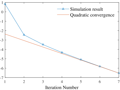
Figure 1: Numerical experiment for regularized PI: $-\ln(\ln(\frac{1}{Ae_{k}}))$ as a function of the iteration number $k$.

For regularized MPI, as shown in (73), $\ln(e_{k})$ is linear with respect to the iteration number $k$, with the slope being $\ln(\gamma^{M})$. So we plot $\ln(e_{k})$ as a function of the number of iterations $k$. The results are shown in Figure 2. The red straight line has the slope $\ln(\gamma^{M})$ and passes through the last data point, which represents the theoretical $\gamma^{M}$ asymptotic linear convergence. We can see that the numerical experiments validate our theoretical result. Note that in this case, we have $\gamma^{M}=0.8^{50}\approx 1.43\times 10^{-5}$. The convergence speed of regularized MPI would have been much underestimated if we only have the previous $\gamma$ linear convergence result [20].

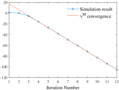
Figure 2: Numerical experiment for regularized MPI: $\ln(e_{k})$ as a function of the iteration number $k$.

VII Conclusion

This paper has shown that regularized policy iteration is strictly equivalent to the standard Newton-Raphson method in the condition of smoothing out Bellman equation with strongly convex functions. This equivalence lays the foundation of a unified analysis for both global and local convergence behaviors of regularized policy iteration. We have shown that regularized policy iteration has global linear convergence with the rate being $\gamma$. Furthermore, this paper has proven for the first time that regularized policy iteration converges quadratically in a local region around the optimal value. We have also shown that regularized modified policy iteration is equivalent to inexact Newton method in which the Newton iteration formula is solved with truncated iterations. This paper has proven for the first time that regularized modified policy iteration achieves an asymptotic linear convergence rate of $\gamma^{M}$ in which $M$ denotes the number of iterations carried out in policy evaluation. The proposed results shed light on the role of regularization in enabling faster convergence for reinforcement learning algorithms.

References

- [1] S. E. Li, Reinforcement Learning for Sequential Decision and Optimal Control. Springer, 2023.
- [2] D. Silver, J. Schrittwieser, K. Simonyan, I. Antonoglou, A. Huang, A. Guez, T. Hubert, L. Baker, M. Lai, A. Bolton et al., “Mastering the game of go without human knowledge,” Nature, vol. 550, no. 7676, pp. 354–359, 2017.
- [3] T. T. Nguyen, N. D. Nguyen, and S. Nahavandi, “Deep reinforcement learning for multiagent systems: A review of challenges, solutions, and applications,” IEEE Transactions on Cybernetics, vol. 50, no. 9, pp. 3826–3839, 2020.
- [4] Y. Guan, Y. Ren, Q. Sun, S. E. Li, H. Ma, J. Duan, Y. Dai, and B. Cheng, “Integrated decision and control: Toward interpretable and computationally efficient driving intelligence,” IEEE Transactions on Cybernetics, vol. 53, no. 2, pp. 859–873, 2023.
- [5] Y. Wen, J. Si, A. Brandt, X. Gao, and H. H. Huang, “Online reinforcement learning control for the personalization of a robotic knee prosthesis,” IEEE Transactions on Cybernetics, vol. 50, no. 6, pp. 2346–2356, 2020.
- [6] J. Li, B. Kiumarsi, T. Chai, F. L. Lewis, and J. Fan, “Off-policy reinforcement learning: Optimal operational control for two-time-scale industrial processes,” IEEE Transactions on Cybernetics, vol. 47, no. 12, pp. 4547–4558, 2017.
- [7] J. Li, J. Ding, T. Chai, and F. L. Lewis, “Nonzero-sum game reinforcement learning for performance optimization in large-scale industrial processes,” IEEE Transactions on Cybernetics, vol. 50, no. 9, pp. 4132–4145, 2019.
- [8] M. L. Puterman, Markov Decision Processes: Discrete Stochastic Dynamic Programming. John Wiley & Sons, 2014.
- [9] M. L. Puterman and S. L. Brumelle, “On the convergence of policy iteration in stationary dynamic programming,” Mathematics of Operations Research, vol. 4, no. 1, pp. 60–69, 1979.
- [10] M. L. Puterman and M. C. Shin, “Modified policy iteration algorithms for discounted markov decision problems,” Management Science, vol. 24, no. 11, pp. 1127–1137, 1978.
- [11] B. Scherrer, M. Ghavamzadeh, V. Gabillon, and M. Geist, “Approximate modified policy iteration,” in International Conference on Machine Learning, 2012, pp. 1889–1896.
- [12] T. Haarnoja, H. Tang, P. Abbeel, and S. Levine, “Reinforcement learning with deep energy-based policies,” in International Conference on Machine Learning, 2017, pp. 1352–1361.
- [13] T. Haarnoja, A. Zhou, P. Abbeel, and S. Levine, “Soft actor-critic: Off-policy maximum entropy deep reinforcement learning with a stochastic actor,” in International Conference on Machine Learning, 2018, pp. 1861–1870.
- [14] J. Duan, Y. Guan, S. E. Li, Y. Ren, Q. Sun, and B. Cheng, “Distributional soft actor-critic: Off-policy reinforcement learning for addressing value estimation errors,” IEEE Transactions on Neural Networks and Learning Systems, vol. 33, no. 11, pp. 6584–6598, 2021.
- [15] G. Xiang and J. Su, “Task-oriented deep reinforcement learning for robotic skill acquisition and control,” IEEE Transactions on Cybernetics, vol. 51, no. 2, pp. 1056–1069, 2019.
- [16] A. Srivastava and S. M. Salapaka, “Parameterized mdps and reinforcement learning problems—a maximum entropy principle-based framework,” IEEE Transactions on Cybernetics, vol. 52, no. 9, pp. 9339–9351, 2021.
- [17] K. Lee, S. Choi, and S. Oh, “Sparse markov decision processes with causal sparse tsallis entropy regularization for reinforcement learning,” IEEE Robotics and Automation Letters, vol. 3, no. 3, pp. 1466–1473, 2018.
- [18] Y. Chow, O. Nachum, and M. Ghavamzadeh, “Path consistency learning in tsallis entropy regularized mdps,” in International Conference on Machine Learning, 2018, pp. 979–988.
- [19] Z. Yang, H. Qu, M. Fu, W. Hu, and Y. Zhao, “A maximum divergence approach to optimal policy in deep reinforcement learning,” IEEE Transactions on Cybernetics, vol. 53, no. 3, pp. 1499–1510, 2023.
- [20] M. Geist, B. Scherrer, and O. Pietquin, “A theory of regularized markov decision processes,” in International Conference on Machine Learning, 2019, pp. 2160–2169.
- [21] Y. Nesterov, “Smooth minimization of non-smooth functions,” Mathematical Programming, vol. 103, no. 1, pp. 127–152, 2005.
- [22] A. Mensch and M. Blondel, “Differentiable dynamic programming for structured prediction and attention,” in International Conference on Machine Learning, 2018, pp. 3462–3471.
- [23] S. Cen, C. Cheng, Y. Chen, Y. Wei, and Y. Chi, “Fast global convergence of natural policy gradient methods with entropy regularization,” Operations Research, vol. 70, no. 4, pp. 2563–2578, 2022.
- [24] J. M. Ortega and W. C. Rheinboldt, Iterative Solution of Nonlinear Equations in Several Variables. SIAM, 2000.
- [25] R. S. Dembo, S. C. Eisenstat, and T. Steihaug, “Inexact newton methods,” SIAM Journal on Numerical Analysis, vol. 19, no. 2, pp. 400–408, 1982.
- [26] S. Boyd, S. P. Boyd, and L. Vandenberghe, Convex Optimization. Cambridge university press, 2004.
- [27] J. Borwein and A. Lewis, Convex Analysis. Springer, 2006.
- [28] J. M. Ortega and W. C. Rheinboldt, “Monotone iterations for nonlinear equations with application to gauss-seidel methods,” SIAM Journal on Numerical Analysis, vol. 4, no. 2, pp. 171–190, 1967.