A Unified Algorithmic Framework for Dynamic Compressive Sensing

Abstract

We propose a unified dynamic tracking algorithmic framework (PLAY-CS) to reconstruct signal sequences with their intrinsic structured dynamic sparsity. By capitalizing on specific statistical assumptions concerning the dynamic filter of the signal sequences, the proposed framework exhibits versatility by encompassing various existing dynamic compressive sensing (DCS) algorithms. This is achieved through the incorporation of a newly proposed Partial-Laplacian filtering sparsity model, tailored to capture a more sophisticated dynamic sparsity. In practical scenarios such as dynamic channel tracking in wireless communications, the framework demonstrates enhanced performance compared to existing DCS algorithms.

I Introduction

In numerous real-time applications, particularly those involving precise dynamic tracking of Millimeter Wave (mmWave) Channel State Information (CSI) within massive Multiple-Input and Multiple-Output (MIMO) systems employing a Hybrid Analog and Digital Beamforming (HBF) architecture[1], a fundamental necessity emerges. This necessity involves the causal reconstruction of time-varying signal sequences based on a restricted set of linear measurements.

Such causal signal reconstruction is sometimes referred to as dynamic filtering[9]. The goal of dynamic filtering is to solve the causal minimum mean squared error (MMSE) estimation of the time-varying signals. The conventional MMSE solution is embodied by the Kalman filter (KF)[3]. However, the standard KF estimation procedure relies on the assumptions of Gaussianity and linearity. They are not often applicable in scenarios where the statistical properties of signals and innovations do not adhere to Gaussian distributions. Furthermore, the KF fails to harness the inherent dynamic structured sparsity within the signal sequence. The challenge of recovering a sparse time-varying signal sequence from a limited number of measurements has been studied for a long time. Often the terms dynamic sparse recovery and dynamic compressive sensing (DCS)[13] are employed interchangeably.

Considering the DCS problem, most of the solutions for this matter consist of batch algorithms[14, 15]. Nevertheless, these algorithms are offline, thereby rendering them computationally unviable for implementation in the MIMO systems. Furthermore, their memory requisites assume prohibitively large proportions when applied within such expansive systems. Additionally, these batch algorithms operate under the assumption that the support set of sparse signals remains static over time, a premise that frequently deviates from practical reality. Therefore, it is indispensable to design recursive algorithms for solving these issues.

Recursive algorithms offer a notable advantage over batch techniques in terms of reduced computational and storage complexity. They are frequently adopted to integrate the observation model and prior information within a unified framework. Thus far, a series of DCS methods have been proposed [4, 5, 6, 8, 9, 16, 17, 18, 19], as summarized below.

Algorithms exploiting the slow support changing characteristic of the dynamic signal: The LS-CS algorithm [5] can be viewed as the first solution that only exploited the slow support changing feature of the signal sequence. It starts to compute an initial LS estimate of the signal on the estimated support set and then executes an $\ell_{1}$-norm minimization on the signal residual. However, the reconstruction performance of the LS-CS relies on the accurate estimation of the support set, which is difficult to satisfy in practical applications. In [6], the sparse recovery problem becomes one of trying to find the solution that is the sparsest outside the support set among all solutions that satisfy the measurement constraint. This is referred to as the Modified-CS algorithm. A proposition in [6] states that the Modified-CS can exactly recover the signal with fewer independent columns of measurement matrix than the Regular-CS[2], i.e., a CS algorithm that reconstructs each sparse signal in the dynamic sequence independently without using any prior information. This is a weaker requirement than the Regular-CS when the predetermined support set at each time slot is estimated accurately enough. The idea of Modified-CS can also be used to modify the greedy approaches for sparse recovery. This has been done in work [16, 17]. They have developed and evaluated OMP with partially known support (OMP-PKS)[16], Compressive Sampling Matching Pursuit (CoSaMP)-PKS and IHT-PKS [17]. Moreover, Modified-CS can be viewed as the relaxation of the Regular-CS, and a special case of Weighted-$\ell_{1}$[9, 18, 19]. The concept behind Weighted-$\ell_{1}$ involves dividing the index set into distinct subsets and applying varying weights to the $\ell_{1}$ norm within each of these subsets. Furthermore, Modified-CS can be viewed as a special case of the Weighted-$\ell_{1}$ when the partition number is two. In [19], some performance guarantees are also obtained for the two set partition case. [19] established a RIP-based Weighted-$\ell_{1}$ exact recovery theorem, which reveals the exact recovery condition among Weighted-$\ell_{1}$, Modified-CS and Regular-CS. [9] derives a reweighted-$\ell_{1}$ minimization problem based on the dynamic filter and shows a similar reweighted scheme to that in [10].

Algorithms exploiting the slow support and value changing characteristic of the dynamic signal: In [4], a Kalman-filter type method is established. It is referred to as KF-CS. The key idea of KF-CS is to evaluate a reduced Kalman filter procedure in the support set and a reduced CS addition detection on the filtering error outside the support. of the slow-changing signal sparsity pattern and a simple spatially i.i.d. Gaussian random walk prior signal model on temporal dynamics, which are impractical in actual scenarios. In [8], an extension algorithm of Modified-CS was proposed to further exploit the signal value slow-changing characteristic. This method is referred to as RegModCS, which adds a regularization on the optimization objective function to further exploit the signal value prior.

Nonetheless, these methods fall short of fully harnessing the inherent sparsity within the dynamic filtering structure While studies such as [11, 12] delve into the hierarchical structured sparsity of the signal itself, they do not effectively capitalize on dynamic structured sparsity, a pivotal aspect in the reconstruction of dynamic signal sequences. Consequently, the need arises for the development of a more sophisticated dynamic signal model and a more efficient algorithmic DCS framework, catering to constructing dynamic structured sparse signal sequences.

In the expansive literature on DCS analysis, it is not yet fully understood whether these existing recursive DCS algorithms have some intrinsical correlations or not. It turns out the answer is yes in this paper. By introducing a structured sparsity model on the dynamic filter, we construct a unified DCS algorithmic framework that can provide further insights into the existing DCS algorithms. Furthermore, we demonstrate that through the application of this novel framework, we can obtain a variant of DCS algorithms that surpasses the performance of its existing counterparts. The main contributions are summarized below.

• Partial-Laplacian filtering sparsity model: We propose a new statistical model called the Partial-Laplacian filtering sparsity model to capture the structured sparsity on the dynamic filter. The Partial-Laplacian model has the flexibility to model the dynamic filtering characteristics of the practical signal sequences.

• Unified DCS algorithmic framework: By combining the methodology of the Kalman filter and the proposed Partial-Laplacian model, we propose a unified DCS algorithmic framework called the Partial Laplacian Dynamic CS (PLAY-CS). PLAY-CS can reveal the correlations among the existing DCS algorithms.

• Specific algorithm design for practical applications: We demonstrate that our newly developed algorithmic framework enables the derivation of a diverse set of DCS algorithms rooted in the proposed Partial Laplacian scale mixture (Partial-LSM) sparsity model. We designate the novel DCS algorithm as $\text{PLAY}^{+}$-CS. Our experiments reveal that $\text{PLAY}^{+}$-CS outperforms existing DCS algorithms in practical applications involving dynamic channel reconstruction.

The rest of the paper is organized as follows. In Section II, we present the problem definition, the system model and the applications of the DCS problem. In section III, we introduce the proposed Partial-Laplacian model and the unified DCS algorithmic framework: PLAY-CS. PLAY-CS shows the connections among the existing DCS algorithms. Then, we derive a more efficient DCS algorithm, called $\text{PLAY}^{+}$-CS. Simulation results and conclusion are given in Section IV and V, respectively.

Notation: The notation $\|x\|_{k}$ denotes the $\ell_{k}$ norm of the vector $x$. $A^{-1},A^{T}$ and $A^{H}$ denote the inverse, transpose and conjugate transpose of matrix $A$, respectively. For a set $T$, we use $T^{c}$ to denote the complement of $T$. $|T|$ denotes the cardinality of the set $T$. We use the notation $A_{T}$ to denote the sub-matrix containing the columns of $A$ with indexes belonging to $T$. For a vector $x$, the notation $(x)_{T}$ refers to a sub-vector that contains the elements with indexes in $T$.

II Problem

II-A Problem Definition

The main goal of DCS problem is to recursively reconstruct a high dimensional sparse $N$-length vector signal sequences $\{x_{t}\}$ from potentially noisy and undersampled $M$-length measurements $\{y_{t}\}$(i.e., $M\ll N$) satisfying

$$y_{t}=A_{t}x_{t}+n_{t},n_{t}\sim\mathcal{CN}(0,R_{t}),$$ (1)

where $A_{t}:=G_{t}\Phi\in\mathbb{C}^{M\times N}$ and $n_{t}$ is a complex Gaussian noise vector with covariance $R_{t}$. Here $G_{t}$ is the measurement matrix and $\Phi$ is a dictionary matrix for the sparsity basis. In the formulation above, $z_{t}:=\Phi x_{t}$ is actually the signal of interest at time $t$, where $x_{t}$ is its representation in the sparsity basis $\Phi$.

II-B System Model

In this paper, we focus on the time-varying signal that has the following dynamic model:

$$x_{t}=f_{t}(x_{t-1})+\nu_{t},$$ (2)

where $f_{n}(\cdot):\mathbb{C}^{N}\to\mathbb{C}^{N}$ is the dynamic function and $\nu_{t}$ is the filtering noise (innovation) that represents the evolving noise in the dynamic model $f_{n}(\cdot)$.

Most standard dynamic filtering techniques are based on the Kalman filter, which often models the dynamic function as a linear version and assumes the filtering noise $\nu_{t}$ is a complex Gaussian noise vector with covariance $Q_{t}$:

$$x_{t}=F_{t}x_{t-1}+\nu_{t},\nu_{t}\sim\mathcal{CN}(0,Q_{t}),$$ (3)

where $F_{t}\in\mathbb{C}^{N\times N}$ is the linear version of the dynamic function $f_{n}(\cdot)$.

In our work, we propose the Partial-Laplacian sparsity model, which extended the model (3) to a more general case. Moreover, we can easily derive a more efficient algorithmic procedure to reconstruct the signal sequences based on this model.

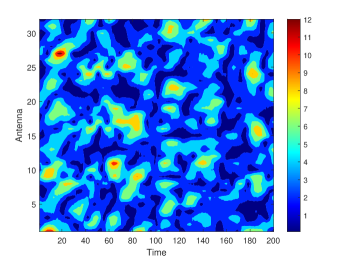
(a)

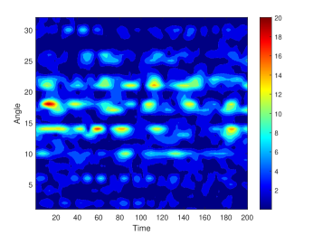
(b)

Figure 1: The channel gains of the CDL-B channel in different domains. (a) Antenna-Time domain. (b) Angle-Time domain.

II-C Applications

The above DCS problem formulation embraces many applications such as dynamic MRI [20], video tracking[21], and speech/audio reconstruction [19]. Besides the above, the DCS problem can also be exploited for the dynamic channel tracking of wireless CSI in MIMO systems[1]. In the following, we consider an example of dynamic channel tracking.

We first consider a narrowband massive MIMO system with HBF [22], where the BS is equipped with $N_{\text{r}}\gg 1$ antennas and $N_{\text{RF}}$ radio frequency (RF) chains, where $N_{\text{r}}\gg N_{\text{RF}}$. The channel $H_{t}\in\mathbb{C}^{N}$ at each time slot $t$ is precoded through an $N_{\text{RF}}\times N_{\text{r}}$ analog beamforming $W_{t}$, which can be generated by discrete Fourier transform (DFT) matrix.

Due to the clustering characteristic of the mmWave propagation [23], the channel is modeled with $N_{L}$ paths. Considering the mmWave system with a half-wave spaced uniform linear array (ULA) at the receiver, the channel vector $H_{t}$ can be represented as

$$H_{t}=\sum_{i=1}^{N_{L}}\alpha_{i}\text{a}(\theta_{i}^{t}),$$ (4)

where $\alpha_{i}$ denoted the complex gain of the $i$th path and $\text{a}(\theta_{i}^{t})=\frac{1}{\sqrt{N_{\text{r}}}}[1\ \ e^{j\pi\sin{\theta_{i}^{t}}}\ \ ...\ \ e^{j\pi(N_{\text{r}}-1)\sin{\theta_{i}^{t}}}]^{T}$ denotes the normalized responses of the receive antenna arrays to the $i$th path at time slot $t$, where $\theta_{i}^{t}$ denotes the angles of arrival.

The observed precoded channel $h_{t}\in\mathbb{C}^{N_{\text{RF}}}$ at time slot $t$ can be represented as

$$h_{t}=W_{t}H_{t}+n_{t},n_{t}\sim\mathcal{CN}(0,\sigma_{m}^{2}{I}_{N_{\text{RF}}}),$$ (5)

where $n_{t}$ is a complex Gaussian noise vector with covariance $\sigma_{m}^{2}{I}_{N_{\text{RF}}}$. Noticing the clustering structure of the channel, $H_{t}$ can be transformed into the sparse angle domain, i.e., $H_{t}$ can be expressed as

$$H_{t}=\text{D}\tilde{H}_{t},$$ (6)

where D is the transform dictionary determined by the geometrical structure of the antenna array, and $\tilde{H}_{t}$ is the sparse representation of the channel in the angle domain. The channel sequences $\{\tilde{H}_{t}\}$ in the angle domain exhibit strong structured dynamic sparsity, as depicted in Fig. 1. In this paper, we focus on the ULA at BS, where D is the DFT matrix. Our discussion can be readily extended to a uniform planner array (UPA) or a more sophisticated antenna array. Substituting (6) and letting $A_{t}=W_{t}\text{D}$, we can rewrite (5) as

$$h_{t}=A_{t}\tilde{H}_{t}+n_{t},$$ (7)

which has the same problem formulation as the DCS problem (1). Our goal is to recursively reconstruct the uplink channel sequence $\{H_{t}\}$ from the low-dimensional observed precoded channel sequence $\{h_{t}\}$.

III Algorithmic Framework

III-A Kalman Filter

The Kalman filter[4] reformulated the above problem as causal minimum mean squared error (MMSE) estimation. If the support is set, the Kalman filter provides the MMSE solution. In the Kalman filter framework, the signal at each time step is recovered using the estimate of previous time step $\hat{x}_{t-1}$ and a calculated covariance for that estimate $P_{t-1}$. The Kalman filter is typically depicted as comprising two phases: prediction and update.

Prediction:

$$\hat{x}_{t|t-1} =F_{t}\hat{x}_{t-1},$$ (8)

$$P_{t|t-1} =F_{t}P_{t-1}F_{t}^{H}+Q_{t},$$ (9)

where $P_{t}$ is $\mathbb{E}[(x_{t}-\hat{x}_{t})(x_{t}-\hat{x}_{t})^{H}]$ and $P_{t|t-1}$ is $\mathbb{E}[(x_{t}-\hat{x}_{t|t-1})(x_{t}-\hat{x}_{t|t-1})^{H}]$.

Update:

$$K =P_{t|t-1}A_{t}^{H}(A_{t}P_{t|t-1}A_{t}^{H}+R_{t})^{-1},$$ (10)

$$\hat{x}_{t} =\hat{x}_{t|t-1}+K(y_{t}-y_{t|t-1}),y_{t|t-1}=A_{t}\hat{x}_{t|t-1},$$ (11)

$$P_{t} =(I-KA_{t})P_{t|t-1},$$ (12)

where $K$ is the Kalman gain.

When it is assumed that measurement noise $R_{t}$ and filtering noise $Q_{t}$ follow a Complex Gaussian distribution, the MMSE estimate of the signal is equivalent to the maximum a posteriori (MAP) estimate. Using the Bayes’ rule we have $p(x_{t}|y_{t})\propto p(y_{t}|x_{t})p(x_{t})$, and therefore the MAP estimate $\hat{x}_{t}$ is given by

$$\hat{x}_{t}=\arg\min_{x}\{\|y_{t}-A_{t}x\|_{R_{t}^{-1}}^{2}+\|x-\hat{x}_{t|t-1}\|_{P_{t|t-1}^{-1}}^{2}\},$$ (13)

where the matrix weighted norm is defined as $\|z\|_{R}^{2}=z^{H}Rz$. Although the optimization in (13) relies solely on local information, the Kalman filter addresses a global optimization problem. However, this characteristic arises from the linearity of the measurement and dynamics functions, along with the Gaussian distribution of both measurement and filtering noise.

In cases where the linearity and Gaussianity conditions are not met, it is necessary to extend the Kalman filter to a more general algorithmic framework. In this study, we firstly propose the Partial-Laplacian filtering sparsity model. Moreover, we found the new algorithmic framework based on the Partial-Laplacian model has a close relationship with the existing DCS algorithms[4, 6, 8, 9]. It means that the new framework can degenerate into the existing DCS algorithms in special cases.

III-B Partial-Laplacian Filtering Sparsity Model

Considering the slow-changing characteristic of the signal, which means the values outside the support evolve very sparsely. Inspired by the Compressive Sensing (CS) technique, one important issue is to capture the sparsity of the addition to the support with a proper regularization term, such as $l_{1}$ norm.

To capture the dynamic sparsity outside the support, we propose the Partial-Laplacian filtering sparsity model:

$$(x_{t})_{T_{t-1}} =(F_{t}x_{t-1})_{T_{t-1}}+(\nu_{t})_{T_{t-1}},$$ (14)

$$(x_{t})_{T_{t-1}^{c}} =(F_{t}x_{t-1})_{T_{t-1}^{c}}+(\nu_{t})_{T_{t-1}^{c}},$$

where $T_{t}$ denotes the the support set of $x_{t}$ and let $L=|T_{t}|$. In other words, $T_{t}=[i_{1},i_{2},...,i_{L}]$, where $i_{k}$ are the non-zero coordinates of $x_{t}$. We assume that $(\nu_{t})_{T_{t-1}}\sim\mathcal{CN}(0,Q_{t}^{1})$ and $(\nu_{t})_{T_{t-1}^{c}}$ have independent Laplacian but non-identical distributions with inverse scale $w_{i}$, i.e. $p((\nu_{t})_{i})=\frac{w_{i}}{2}e^{-w_{i}|(\nu_{t})_{i}|},i\in T_{t-1}^{c}$.

Based on the dynamic model (14), the MAP estimate is

$$\hat{x}_{t}=\arg\min_{x} \{\|y_{t}-A_{t}x\|_{R_{t}^{-1}}^{2}+\gamma\|(x)_{T}-(\hat{x}_{t|t-1})_{T}\|_{(P_{t|t-1})_{1}^{-1}}^{2}$$ (15)

$$+\|W_{t}((x)_{T^{c}}-(\hat{x}_{t|t-1})_{T^{c}})\|_{1}\},$$

where the submatrix $(P_{t|t-1})_{1}=\gamma(P_{t|t-1})_{T,T}$ and $W_{t}={\text{diag}}(w_{i_{1}},w_{i_{2}},...,w_{i_{N-L}})$ is a diagonal matrix.

Utilizing the Partial-Laplacian filtering sparsity model as a foundation, we can formulate a comprehensive DCS algorithmic framework called the Partial Laplacian Dynamic CS (PLAY-CS), as outlined in Algorithm 1. This newly developed DCS algorithm can transform into pre-existing DCS algorithms, a demonstration of which will be presented in the subsequent section.

Algorithm 1 Partial Laplacian Dynamic CS (PLAY-CS)

0:  $\{y_{1},y_{2},...,y_{T}\}$, $A_{t},\forall t$, $\sigma_{m}^{2}$, $\sigma_{m}^{2}$, $\alpha$, $a,b$,$F_{t},\forall t$,$W_{t},\forall t$

  Initialize:  $Q_{t}=\sigma_{m}^{2}{I},R_{t}=\sigma_{f}^{2}I,\forall t$, $P_{0}=I,\hat{x}_{0}={0},T_{0}=\emptyset$

  for all $t=1,2,...,T$ do

     Prediction

           $\hat{x}_{t|t-1}=F_{t}\hat{x}_{t-1},$

           $P_{t|t-1}=F_{t}P_{t-1}F_{t}^{H}+Q_{t},$

           $T=T_{t-1}.$

     Update

           $K=P_{t|t-1}A_{t}^{H}(A_{t}P_{t|t-1}A_{t}^{H}+R_{t})^{-1}.$

           Estimate $\hat{x}_{t}$ using (15).

           $P_{t}=(I-KA_{t})P_{t|t-1}.$

           Support estimation: $T_{t}=\{i:|(\hat{x}_{t})_{i}|>\alpha\}$.

  end for

  $\{\hat{x}_{1},\hat{x}_{2},...,\hat{x}_{T}\}$

III-C Connection to Other DCS Algorithms

TABLE I: Summary of the connection between PLAY-CS and existing DCS algorithms

Algorithm	Connections with PLAY-CS
KF-CS	make $(x_{t})_{T}$ and $(x_{t})_{T^{c}}$ independent
Modified-CS	$W_{t}=I,{\hat{x}_{t|t-1}=0},\gamma=0$
RegModCS	$W_{t}=I,(\hat{x}_{t|t-1})_{T^{c}}=0$
Weighted-$\ell_{1}$	$\hat{x}_{t|t-1}=0$,$T=\emptyset$

The proposed PLAY-CS algorithm can reveal the intrinsical correlations of some existing DCS algorithms [4, 6, 8, 9]. Table I shows the connections between the PLAY-CS algorithm and existing DCS algorithms.

KF-CS[4]: Introduced in [4], KF-CS algorithm is employed to solve a recursive dynamic CS problem. The key idea is to run a reduced KF in signals’ estimate support, and then execute a addition detection outside the support by solving the $\ell_{1}$ problem on this residual. We mention that KF-CS can be viewed as a special case of the PLAY-CS under assumption that the filtering noise $(\nu_{t})$ can be divided into two independent parts: $(\nu_{t})_{T}$ and $(\nu_{t})_{T^{c}}$ and $W_{t}=I$. This means the PLAY-CS can be executed through two consecutive steps, which is equivalent to the KF-CS algorithm.

Modified-CS[6]: For the noisy measurement, the solution of the Modified-CS problem[6] is given by

$$\hat{x}_{t}=\arg\min_{x}\|{y}_{t}-A_{t}x\|_{2}^{2}+\|(x)_{T^{c}}\|_{1}.$$ (16)

Assuming $\gamma=0$ and $W_{t}=I$ in (15), the Modified-CS problem can be viewed as a special case of the PLAY-CS.

RegModCS[8]: RegModCS[8] furtherly exploit the slow value changing structure of the DCS problem by adding a slow value change penalty item to the Modified-CS

$$\hat{x}_{t}=\arg\min_{x}\|{y}_{t}-A_{t}x\|_{2}^{2}+\gamma\|(x)_{T}-(\hat{x}_{t|t-1})_{T}\|^{2}+\|(x)_{T^{c}}\|_{1},$$ (17)

which can be derived based on the PLAY-CS under the assumption that $W_{t}=I$ and $(\hat{x}_{t|t-1})_{T^{c}}={0}$

Weighted-$\ell_{1}$[9]: Consider the following Weighted-$\ell_{1}$ problem[9]

$$\hat{x}_{t}=\arg\min_{x}\|{y}_{t}-A_{t}x\|_{2}^{2}+\|W_{t}x\|_{1},$$ (18)

which can be viewed as an extension of Modified-CS. Moreover, Weighted-$\ell_{1}$ can be considered a simplified variant of the PLAY-CS. It shares a similar interpretation with Modified-CS when we set $T=\emptyset$.

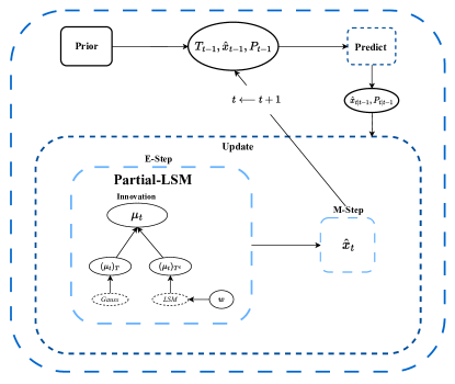
Figure 2: The hierarchical structure of the Partial-LSM model

III-D Partial-LSM Filtering Sparsity Model

Although Partial-Laplacian model is useful for illustrating the signal’s structured dynamic sparsity, parameter $W_{t}$ tuning remains a difficult problem for the proposed algorithm. To address the above issue, the Partial Laplacian scale mixture (Partial-LSM) filtering sparsity model shown as Fig. 2 is proposed in this study.

Firstly, we shall introduce the Laplacian scale mixture (LSM) [12] sparse prior. Given the vector $\lambda$, LSM assumes the signal $x$ have independent but non-identically distributed Laplacian entries, i.e., $p(x\mid\lambda)=\prod_{n=1}^{N}p\left(x_{n}\mid\lambda_{n}\right)$, where

$$p\left(x_{n}\mid\lambda_{n}\right)=\frac{\lambda_{n}}{2}e^{-\lambda_{n}|x_{n}|},\forall n,$$ (19)

and $\lambda_{n},\forall n$ are modeled as independent Gamma distributions, i.e., $p(\lambda)=\prod_{n=1}^{N}p(\lambda_{n})$ with

$$p\left(\lambda_{n}\right)=\Gamma(a,b)=\frac{b^{a}}{\Gamma(a)}\lambda_{n}^{a-1}e^{-b\lambda_{n}},$$ (20)

where $a,b$ are the shape parameter and inverse scale parameter respectively, which are set to promote sparsity of $x$. With this particular choice of a prior on $\lambda$, the distribution over $x_{n}$ is computed by integrating out $\lambda_{n}$ analytically:

$$p\left(x_{n}\right)=\frac{ab^{a}}{2\left(b+\left|x_{n}\right|\right)^{a+1}},$$ (21)

which has heavier tails than the Laplacian distribution. Moreover, due to the conjugacy between Gamma distribution and Laplacian distribution, i.e.,

$$p\left(\lambda_{n}\mid x_{n}\right)=\Gamma(\lambda_{n};a+1,b+|x_{n}|),$$ (22)

we can derive an alternatively iterative algorithmic procedure using the Expectation-Maximization (EM) algorithm.

However, LSM only models the spatial sparsity of the signal itself. In other words, LSM does not consider the dynamic sparsity of filtering noise outside the support, which motivates us to construct the Partial-LSM sparsity model in this study.

In the following, we shall introduce the Partial-LSM sparse prior model to capture the structured sparsity by modeling the filtering noise outside the support with LSM prior.

In model (14), we futher model the inverse scale parameter $w_{i}$ of $(\nu_{t})_{i},i\in T_{t-1}^{c}$ as independent Gamma distributions

$$p\left(w_{i}\right)=\frac{b^{a}}{\Gamma(a)}w_{i}^{a-1}e^{-bw_{i}},i\in T_{t-1}^{c}.$$ (23)

Using Bayes’s rule and the assumption that $(x_{t})_{T}$ and $(x_{t})_{T^{c}}$ are independent, the MAP estimate based on the Partial-LSM model is given by

$$\hat{x}_{t}= \arg\min_{x}\{-\log p(x\mid y_{t})\}$$ (24)

$$= \arg\min_{x}\{-\log p(y_{t}\mid x)-\log p(x)\}$$

$$= \arg\min_{x}\{-\log p(y_{t}\mid x)-\log p((x)_{T})-\log p((x)_{T^{c}})\}$$

In general it is difficult to compute the MAP estimate with the Partial-LSM prior on the filtering noise. However, if we also known the latent variable $w=[w_{i_{1}},w_{i_{2}},...,w_{i_{N-L}}]^{T}$, we would have an objective function that can be minimized with respect to $x$. The typical approach when dealing with such a problem is the EM algorithm.

In the subsequent sections, we will develop an EM algorithm to estimate the MAP value of $x_{t}$. By applying Jensen’s inequality, we can derive the following upper bound for the posterior likelihood.

$$-\log p(x\mid y_{t})\leq -\log p(y_{t}\mid x)-\log p((x)_{T})$$ (25)

$$-\int_{w}q(w)\log\frac{p((x)_{T^{c}},w)}{q(w)}dw:=\mathcal{L}(q,x),$$

which is true for any probability distribution $q(w)$. Employing the EM algorithm as the foundation, we can execute coordinate descent in $\mathcal{L}(q,x)$. This process involves two pivotal updates, commonly referred to as the E step and the M step:

E Step $$q^{(k+1)}=\underset{q}{\arg\min}\mathcal{L}\left(q,x^{(k)}\right),$$ (26)

M Step $$x^{(k+1)}=\underset{x}{\arg\min}\mathcal{L}\left(q^{(k+1)},x\right),$$ (27)

where $k$ denotes the $k$-th iteration step in estimation of $x_{t}$

Let $\langle.\rangle_{q}$ denote the expectation with respect to $q(w)$. The M Step (27) simplifies to (15), where $(W_{t})^{k}={\text{diag}}(\langle w_{i_{1}}\rangle_{q^{k}},\langle w_{i_{2}}\rangle_{q^{k}},...,\langle w_{i_{N-L}}\rangle_{q^{k}})$. In other words, the weight matrix $(W_{t})^{k}$ can be automatically learned using EM algorithm.

We have equality in the Jensen inequality if $q(w)=p(w\mid x)$. The inequality (25) is therefore tight for this particular choice of $q$, which implies that the E step reduces to $q^{(k+1)}(w)=p(w\mid x^{k})$. Note that in the M step we only need to compute the expectation of $w_{i}$ with respect to the distribution $q$ in the E step. Hence we only need to compute the sufficient statistics $\langle w_{i}\rangle_{p(w\mid x^{k})}$.

Based on the Partial-LSM model (23), we can use the fact (22) to compute the sufficient statistics:

$$\langle w_{i}\rangle_{p(w\mid x^{k})}=\frac{a+1}{b+|(x^{k})_{i}|}$$ (28)

The complete optimization procedure for the Partial-LSM DCS ($\text{PLAY}^{+}$-CS) is outlined in Algorithm 2. In the following section, we will present a comparative analysis of simulation results for $\text{PLAY}^{+}$-CS and other DCS algorithms using realistic channel datasets.

Algorithm 2 PLAY-CS with LSM ($\text{PLAY}^{+}$-CS)

0:  $\{y_{1},y_{2},...,y_{T}\}$, $A_{t},\forall t$, $\sigma_{m}^{2}$, $\sigma_{m}^{2}$, $\alpha$, $a,b$,$F_{t},\forall t$

  Initialize:  $Q_{t}=\sigma_{m}^{2}{I},R_{t}=\sigma_{f}^{2}I,\forall t$, $P_{0}=I,\hat{x}_{0}={0},T_{0}=\emptyset$

  for all $t=1,2,...,T$ do

     Prediction

           $\hat{x}_{t|t-1}=F_{t}\hat{x}_{t-1},$

           $P_{t|t-1}=F_{t}P_{t-1}F_{t}^{H}+Q_{t},$

           $T=T_{t-1}.$

     Update

           $K=P_{t|t-1}A_{t}^{H}(A_{t}P_{t|t-1}A_{t}^{H}+R_{t})^{-1}.$

           E-Step

               Set diagonal matrix $W_{t}$ using (28)

           M-Step

               Estimate $\hat{x}_{t}$ using (15).

           $P_{t}=(I-KA_{t})P_{t|t-1}.$

           Support estimation: $T_{t}=\{i:|(\hat{x}_{t})_{i}|>\alpha\}$.

  end for

  $\{\hat{x}_{1},\hat{x}_{2},...,\hat{x}_{T}\}$

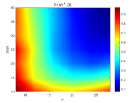
(a)

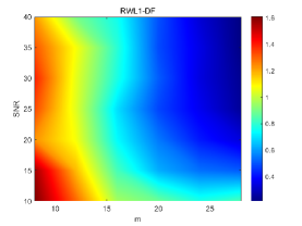
(b)

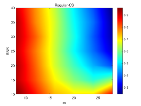
(c)

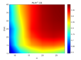
(d)

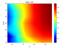
(e)

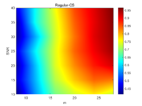
(f)

Figure 3: The TNMSE and TCorr performances of various algorithms under diffirent SNR and CR levels. (a) TNMSE of $\text{PLAY}^{+}$-CS. (b) TNMSE of RWL1-DF. (c) TNMSE of Regular-CS. (d) TCorr of $\text{PLAY}^{+}$-CS. (e) TCorr of RWL1-DF. (f) TCorr of Regular-CS.

IV Simulation Results

IV-A Experimental Setup

Datasets: In this study, we evaluate the performance of the proposed algorithm using the widely used clustered delay line (CDL) channel models as specified in Table 7.7.1-2 (CDL-B) in [24].

Comparison Methods: We compare the proposed method with the following state-of-the-art methods: Regular-CS[2], Modified-CS[6], RegModCS[8], Weighted-$\ell_{1}$[9].

Evaluation Measures: To evaluate the reconstruction performance of the proposed method, four different metrics are employed in this study.

NMSE: The resulting normalized mean squared error (NMSE) at each $t$ was computed by averaging over 100 Monte Carlo simulations of the above model:

$$\text{NMSE}:=\frac{\|\hat{x}_{t}-x_{t}\|^{2}}{\|x_{t}\|^{2}},$$ (29)

Corr: Another important metric to evaluate the reconstruction performance is the correlation (Corr) between $\hat{x}_{t}$ and $x_{t}$ is defined as

$$\text{Corr}:=\frac{\hat{x}_{t}^{H}x_{t}}{\|x_{t}\|\ |\hat{x}_{t}\|},$$ (30)

which is a useful performance metric in practical applications, such as channel reconstruction.

TNMSE/TCorr: The average performance metrics that we utilized to analyze the reconstruction performance, which we refer to as the time-averaged NMSE (TNMSE) and time-averaged Corr (TCorr), are defined as

$$\text{TNMSE}:=\frac{1}{T}\sum_{t=1}^{T}\frac{\|\hat{x}_{t}-x_{t}\|^{2}}{\|x_{t}\|^{2}},$$ (31)

$$\text{TCorr}:=\frac{1}{T}\sum_{t=1}^{T}\frac{\hat{x}_{t}^{H}x_{t}}{\|x_{t}\|\ |\hat{x}_{t}\|},$$ (32)

where $T$ is the length of the overall signal sequences. Generally, larger Corr, TCorr and smaller NMSE, TNMSE indicate higher reconstruction accuracy.

IV-B Performance Comparison with Other Methods

For the channel reconstruction, We simulated a 200 consecutive time sequence of CDL-B dataset. Under various number of measurement numbers, different levels of additive Gaussian white noise are added into the measurements, which result in the different levels of compression rate (CR) (i.e., the ratio of $m$ to $n$) and signal noise ratio (SNR) of measurements. Regular-CS, Mod-CS, RegMod-CS, and RWL1-DF are implemented as the comparison methods. Given the corresponding noisy measurements $y_{t}$ and random measurement matrix $A_{t}$, we recover the signal $\hat{x}_{t}$ under different levels of CR and SNR.

Under two different levels of SNR, the NMSE curves and Corr curves versus time slot of different methods are plotted in Fig. 4 and Fig. 5. It can be seen that $\text{PLAY}^{+}$-CS outperform all other methods on CDL-B dataset. For example, when SNR=40db and $m=24$, $\text{PLAY}^{+}$-CS exceeds other competing DCS methods on TNMSE at least by 4.6db on the CDL-B dataset. The improvement of $\text{PLAY}^{+}$-CS comes from capturing the underlying structured dynamic sparsity in the sparse signal sequences.

Compared with RWL1-DF and Regular-CS under a wide range of SNR and number of measurements $m$, the TNMSE and TCorr performance are shown in Fig. 3. From Fig. 3, we see that the proposed $\text{PLAY}^{+}$-CS algorithm can achieve a considerable gain over the existing DCS algorithms under various system settings.

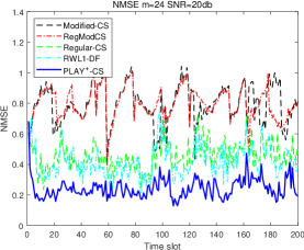
(a)

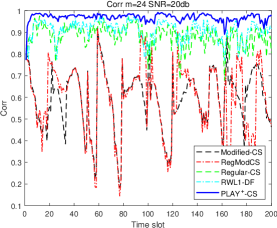
(b)

Figure 4: The NMSE curves and Corr curves of different methods when SNR of measurements is 20db and $m=24$. (a) TNMSE curves. (b) TCorr curves.

(a)

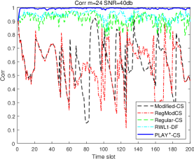
(b)

Figure 5: The NMSE curves and Corr curves of different methods when SNR of measurements is 40db and $m=24$. (a) TNMSE curves. (b) TCorr curves.

IV-C Impact of SNR

Table II and Table IV give the comparison results on TNMSE under different CR levels. Concurrently, Table III and Table V give the comparison results on TCorr across varying CR levels. It is observed that $\text{PLAY}^{+}$-CS outperforms other comparison methods on the CDL-B dataset, yielding lower TNMSE and higher TCorr scores. More specifically, when the value of $m$ is set to 24 or 16, both TNMSE and TCorr performances of $\text{PLAY}^{+}$-CS surpass those of all other DCS algorithms.

TABLE II: The TNMSE of different methods when $m=16$

	SNR=15	SNR=20	SNR=25	SNR=30	SNR=35	SNR=40
Modified-CS	0.6949	0.6618	0.6545	0.6575	0.6609	0.6482
RegModCS	0.8802	0.8508	0.8441	0.8609	0.8792	0.8639
Regular-CS	0.8336	0.8141	0.8193	0.8433	0.8183	0.8018
RWL1-DF	0.8332	0.7361	0.6956	0.7735	0.7940	0.7594
$\text{PLAY}^{+}$-CS	0.4917	0.3976	0.3385	0.3452	0.3531	0.3469

TABLE III: The TCorr of different methods when $m=16$

	SNR=15	SNR=20	SNR=25	SNR=30	SNR=35	SNR=40
Modified-CS	0.7178	0.7379	0.7408	0.7326	0.7395	0.7533
RegModCS	0.5348	0.5897	0.5764	0.5269	0.5981	0.5954
Regular-CS	0.5118	0.5606	0.5624	0.5239	0.5294	0.5293
RWL1-DF	0.6967	0.7421	0.7691	0.7089	0.7138	0.7247
$\text{PLAY}^{+}$-CS	0.8789	0.9175	0.9403	0.9360	0.9348	0.9361

TABLE IV: The TNMSE of different methods when $m=24$

	SNR=15	SNR=20	SNR=25	SNR=30	SNR=35	SNR=40
Modified-CS	0.5379	0.4562	0.4100	0.3937	0.4100	0.3877
RegModCS	0.8152	0.7954	0.8032	0.8250	0.7795	0.8255
Regular-CS	0.7977	0.7977	0.7724	0.8260	0.7870	0.7759
RWL1-DF	0.5414	0.4186	0.3678	0.3456	0.3536	0.3307
$\text{PLAY}^{+}$-CS	0.4366	0.2432	0.1790	0.1438	0.1259	0.1150

TABLE V: The TCorr of different methods when $m=24$

	SNR=15	SNR=20	SNR=25	SNR=30	SNR=35	SNR=40
Modified-CS	0.8426	0.8830	0.9019	0.9119	0.9080	0.9124
RegModCS	0.5816	0.5908	0.6048	0.5421	0.6046	0.5953
Regular-CS	0.5831	0.5953	0.6053	0.5432	0.6244	0.5621
RWL1-DF	0.8595	0.9093	0.9253	0.9358	0.9344	0.9419
$\text{PLAY}^{+}$-CS	0.9098	0.9689	0.9823	0.9885	0.9914	0.9925

IV-D Impact of CR

In Fig. 6 and Fig. 7, We present a comparative analysis of TNMSE and TCorr performance for various algorithms versus the number of measurements $m$ under varying noise levels, specifically at 20 dB and 40 dB. The proposed $\text{PLAY}^{+}$-CS algorithm demonstrates a substantial performance improvement when compared to various other DCS algorithms. This improvement is observed across a range of SNR values and different values of $m$. This demonstrates the $\text{PLAY}^{+}$-CS’s superior ability to effectively track dynamic channels in a massive MIMO system by exploiting channel dynamic sparsity.

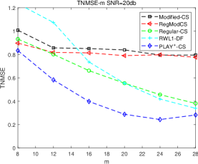
(a)

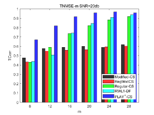
(b)

Figure 6: The TNMSE curves and TCorr bar charts of different methods when SNR of measurements is 20db. (a) TNMSE curves. (b) TCorr bar charts.

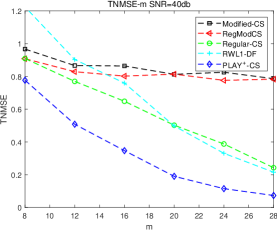
(a)

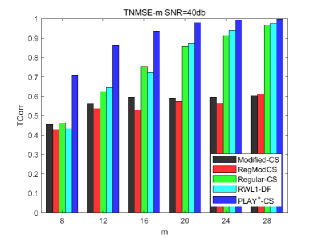
(b)

Figure 7: The TNMSE curves and TCorr bar charts of different methods when SNR of measurements is 40db. (a) TNMSE curves. (b) TCorr bar charts.

V Conclusions and Future Work

This study addresses the dynamic channel tracking problem in a massive MIMO system. First, we introduce the Partial-Laplacian, a dynamic channel statistical model, to represent the structured dynamic sparsity of massive MIMO channels. Next, we present a unified DCS framework (PLAY-CS) for dynamic channel tracking algorithms that uncovers inherent correlations among existing DCS algorithms. Furthermore, leveraging the Partial-LSM filtering sparsity model, we develop a variant of the DCS algorithm called $\text{PLAY}^{+}$-CS. We validate the excellent performance of the $\text{PLAY}^{+}$-CS using the CDL-B channel dataset for the dynamic tracking of massive MIMO channels. Extensive simulations demonstrate that $\text{PLAY}^{+}$-CS effectively harnesses the structured dynamic sparsity inherent in practical massive MIMO channels, resulting in significant improvements over various existing DCS algorithms.

Finally, although we have exclusively focused on frequency-flat fading channels in this paper, our proposed method can be extended to reconstruct frequency-selective fading channels. This can be achieved through a combination of MMV technology and our proposed algorithm or by exploiting structured sparsity in the delay/frequency domain. A promising avenue for future research is the development of a suitable probability model that can jointly capture structured sparsity in the spatial/delay/frequency domain and the temporal domain. Our proposed algorithmic framework can be extended to address the more practical problem of tracking frequency-selective fading channels with a more general statistical channel model in future research.

References

- [1] Larsson E G, Edfors O, Tufvesson F, et al. Massive MIMO for next generation wireless systems[J]. IEEE communications magazine, 2014, 52(2): 186-195.
- [2] Chen S S, Donoho D L, Saunders M A. Atomic decomposition by basis pursuit[J]. SIAM review, 2001, 43(1): 129-159.
- [3] Kalman R E. A new approach to linear filtering and prediction problems[J]. 1960.
- [4] Vaswani N. Kalman filtered compressed sensing[C]//2008 15th IEEE International Conference on Image Processing. IEEE, 2008: 893-896.
- [5] Vaswani N. LS-CS-residual (LS-CS): Compressive sensing on least squares residual[J]. IEEE Transactions on Signal Processing, 2010, 58(8): 4108-4120.
- [6] Vaswani N, Lu W. Modified-CS: Modifying compressive sensing for problems with partially known support[J]. IEEE Transactions on Signal Processing, 2010, 58(9): 4595-4607.
- [7] Lu W, Vaswani N. Modified compressive sensing for real-time dynamic MR imaging[C]//2009 16th IEEE International Conference on Image Processing (ICIP). IEEE, 2009: 3045-3048.
- [8] Lu W, Vaswani N. Regularized modified BPDN for noisy sparse reconstruction with partial erroneous support and signal value knowledge[J]. IEEE Transactions on Signal Processing, 2011, 60(1): 182-196.
- [9] Charles A S, Rozell C J. Dynamic filtering of sparse signals using reweighted [C]//2013 IEEE International Conference on Acoustics, Speech and Signal Processing. IEEE, 2013: 6451-6455.
- [10] Candes E J, Wakin M B, Boyd S P. Enhancing sparsity by reweighted minimization[J]. Journal of Fourier analysis and applications, 2008, 14: 877-905.
- [11] Zhang L, Wei W, Tian C, et al. Exploring structured sparsity by a reweighted Laplace prior for hyperspectral compressive sensing[J]. IEEE Transactions on Image Processing, 2016, 25(10): 4974-4988.
- [12] Garrigues P, Olshausen B. Group sparse coding with a laplacian scale mixture prior[J]. Advances in neural information processing systems, 2010, 23.
- [13] Vaswani N, Zhan J. Recursive recovery of sparse signal sequences from compressive measurements: A review[J]. IEEE Transactions on Signal Processing, 2016, 64(13): 3523-3549.
- [14] Wipf D P, Rao B D. An empirical Bayesian strategy for solving the simultaneous sparse approximation problem[J]. IEEE Transactions on Signal Processing, 2007, 55(7): 3704-3716.
- [15] Tropp J A. Algorithms for simultaneous sparse approximation. Part II: Convex relaxation[J]. Signal Processing, 2006, 86(3): 589-602.
- [16] Stanković V, Stanković L, Cheng S. Compressive image sampling with side information[C]//2009 16th IEEE International Conference on Image Processing (ICIP). IEEE, 2009: 3037-3040.
- [17] Carrillo R E, Polania L F, Barner K E. Iterative algorithms for compressed sensing with partially known support[C]//2010 IEEE International Conference on Acoustics, Speech and Signal Processing. IEEE, 2010: 3654-3657.
- [18] Khajehnejad M A, Xu W, Avestimehr A S, et al. Weighted minimization for sparse recovery with prior information[C]//2009 IEEE international symposium on information theory. IEEE, 2009: 483-487.
- [19] Friedlander M P, Mansour H, Saab R, et al. Recovering compressively sampled signals using partial support information[J]. IEEE Transactions on Information Theory, 2011, 58(2): 1122-1134.
- [20] Martin A, Weber O, Saloner D, et al. Application of MR technology to endovascular interventions in an XMR suite[J]. Medicamundi, 2002, 46(3): 28-35.
- [21] Cevher V, Sankaranarayanan A, Duarte M F, et al. Compressive sensing for background subtraction[C]//Computer Vision–ECCV 2008: 10th European Conference on Computer Vision, Marseille, France, October 12-18, 2008, Proceedings, Part II 10. Springer Berlin Heidelberg, 2008: 155-168.
- [22] Lin T, Cong J, Zhu Y, et al. Hybrid beamforming for millimeter wave systems using the MMSE criterion[J]. IEEE Transactions on Communications, 2019, 67(5): 3693-3708.
- [23] El Ayach O, Rajagopal S, Abu-Surra S, et al. Spatially sparse precoding in millimeter wave MIMO systems[J]. IEEE transactions on wireless communications, 2014, 13(3): 1499-1513.
- [24] Study on Channel Model for Frequencies From 0.5 to 100 GHz, document TR 38.901 V15.0.0, 3GPP, Jun. 2018.