SpikePoint: An Efficient Point-based Spiking Neural Network for Event Cameras Action Recognition
Abstract
Event cameras are bio-inspired sensors that respond to local changes in light intensity and feature low latency, high energy efficiency, and high dynamic range. Meanwhile, Spiking Neural Networks (SNNs) have gained significant attention due to their remarkable efficiency and fault tolerance. By synergistically harnessing the energy efficiency inherent in event cameras and the spike-based processing capabilities of SNNs, their integration could enable ultra-low-power application scenarios, such as action recognition tasks. However, existing approaches often entail converting asynchronous events into conventional frames, leading to additional data mapping efforts and a loss of sparsity, contradicting the design concept of SNNs and event cameras. To address this challenge, we propose SpikePoint, a novel end-to-end point-based SNN architecture. SpikePoint excels at processing sparse event cloud data, effectively extracting both global and local features through a singular-stage structure. Leveraging the surrogate training method, SpikePoint achieves high accuracy with few parameters and maintains low power consumption, specifically employing the identity mapping feature extractor on diverse datasets. SpikePoint achieves state-of-the-art (SOTA) performance on five event-based action recognition datasets using only 16 timesteps, surpassing other SNN methods. Moreover, it also achieves SOTA performance across all methods on three datasets, utilizing approximately 0.3% of the parameters and 0.5% of power consumption employed by artificial neural networks (ANNs). These results emphasize the significance of Point Cloud and pave the way for many ultra-low-power event-based data processing applications.
1 Introduction
Event camera is a recent development in computer vision, and it is revolutionizing the way visual information is captured and processed (Gallego et al., 2020). They are particularly well-suited for detecting fast-moving objects, as they can eliminate redundant information and significantly reduce memory usage and data processing requirements. This is achieved through innovative pixel design, resulting in a sparse data output that is more efficient than traditional cameras (Posch et al., 2010; Son et al., 2017). However, most of the event data processing algorithms rely on complex and deep ANNs, which are not aligned with the event camera’s low power consumption benefits. Instead, combining event-based vision tasks with SNNs has shown great potential thanks to their highly compatible properties, especially in tasks such as action recognition(Liu et al., 2021a).
Spiking Neural Networks have emerged as a promising alternative that can address the limitations of traditional neural networks for their remarkable biological plausibility, event-driven processing paradigm, and exceptional energy efficiency (Gerstner & Kistler, 2002). The network’s asynchronous operations depend on biological neurons, communicating information via precisely timed discrete spikes (Neftci et al., 2019). The event-driven processing paradigm enables sparse but potent computing capabilities, where a neuron activates only when it receives or generates a spike (Hu et al., 2021). This property gives the network remarkably high energy efficiency and makes it an ideal candidate for processing event-based data. Nevertheless, existing approaches for combining event cameras with SNN require the conversion of asynchronous events into conventional frames for downstream processing, resulting in additional data mapping work and a loss of sparsity (Kang et al., 2020)(Berlin & John, 2020). Moreover, this process leads to the loss of detailed temporal information, which is critical for accurate action recognition (Innocenti et al., 2021). Therefore, developing SNN-compatible novel techniques that operate directly on event data remains challenging.
Point Cloud is a powerful representation of 3D geometry that encodes spatial information in the form of a sparse set of points and eliminates the need for the computational image or voxel conversion, making it an efficient and ideal choice for representing event data (Qi et al., 2017a). The sparse and asynchronous event data could be realized as a compact and informative 3D space-time representation of the scene, bearing a resemblance to the concept of Point Cloud (Sekikawa et al., 2019). Still, Point Cloud networks need frequent high-data dimension transformations and complex feature extraction operators in ANNs. Due to their binarization and dynamic characteristics, these may not function optimally in SNNs.
In this paper, we introduce SpikePoint, the first point-based Spiking Neural Network for effectively and efficiently processing event data in vision-based tasks. Our contributions are as follows: First, we combine event-based vision tasks with SNN by treating the input as Point Clouds rather than stacked event frames to preserve the fine-grained temporal feature and retain the sparsity of raw events. Second, unlike ANN counterparts with a multi-stage hierarchical structure, we design a singular-stage structure harnessing SNN to effectively extract local and global features. This lightweight design achieves effective performance through the back-propagation training method. Lastly, we introduce a pioneering encoding approach to address relative position data containing negative values within the point cloud. This scheme maintains symmetry between positive and negative values, optimizing information representation. We evaluate SpikePoint on diverse event-based action recognition datasets of varying scales, achieving SOTA results on Daily DVS (Liu et al., 2021a), DVS ACTION (Miao et al., 2019), HMDB51-DVS datasets, surpassing even traditional ANNs. Additionally, we attain the SNN’s SOTA on the DVS128 Gesture (Amir et al., 2017) and UCF101-DVS dataset (Bi et al., 2020). Notably, our evaluation encompasses an assessment of network power consumption. Compared to both SNNs and ANNs with competitive accuracy, our framework consistently exhibits exceptional energy efficiency, both in dynamic and static power consumption, reaffirming the unequivocal superiority of our network.
2 Related Work
2.1 Event-based action recognition
Action recognition is a critical task with diverse applications in anomaly detection, entertainment, and security. Two primary methods for event-based action recognition are ANN and SNN (Ren et al., 2023). The ANN approaches have yielded several notable contributions, including IBM’s pioneering end-to-end gesture recognition system (Amir et al., 2017) and Cannici’s asynchronous event-based full convolutional networks (Cannici et al., 2019), while Chadha et al. developed a promising multimodal transfer learning framework for heterogeneous environments (Chadha et al., 2019). Additionally, Bin Yin et al. proposed a graph-based spatiotemporal feature learning framework and introduced several new datasets (Bi et al., 2020), including HMDB51-DVS. (Ren et al., 2023) proposed an effective lightweight framework to deal with event-based action recognition using a tensor compression approach, and (Shen et al., 2023) proposed an efficient data augmentation strategy for event stream data. On the other hand, SNN methods have also demonstrated great potential, with Liu et al. presenting a successful model for object classification using address event representation (Liu et al., 2020) and (George et al., 2020) using multiple convolutional layers and a reservoir to extract spatial and temporal features, respectively. (Liu et al., 2021a) have further advanced the field by extracting motion information from asynchronous discrete events captured by event cameras, and (Yao et al., 2023) developed the Refine-and-Mask SNN (RM-SNN), characterized by its self-adaptive mechanism to modulate spiking responses based on data input. While these SNNs have improved in terms of efficiency, however, their accuracy still falls short when compared to ANN-based approaches.
2.2 Point Cloud networks in ANN
Point-based methods have revolutionized the direct processing of Point Cloud data as input, with PointNet (Qi et al., 2017a) standing out as a remarkable example. PointNet++ (Qi et al., 2017b) took it a step further by introducing a set abstraction module. While it used a simple MLP in the feature extractor, numerous more advanced feature extractors have recently been developed to elevate the quality of Point Cloud processing (Wu et al., 2019; Zhao et al., 2021; Ma et al., 2021; Dosovitskiy et al., 2020; Zhang et al., 2023; Qian et al., 2022; Wu et al., 2023). To apply these methods to the event stream, Wang et al. (Wang et al., 2019) first tackled the temporal information processing challenge while preserving representation in both the x and y axes, achieving gesture recognition using PointNet++. PAT (Yang et al., 2019) further improved this model by incorporating self-attention and Gumbel subset sampling, achieving even better performance in the recognition task. Nonetheless, the current performance of the point-based models still cannot compete with frame-based methods in terms of accuracy. Here, we propose SpikePoint as a solution that fully leverages the characteristics of event clouds while maintaining high accuracy, low parameter numbers, and low power consumption.
3 SpikePoint
3.1 Event cloud
Event streams are time-series data that record spatial intensity changes in chronological order. Each event can be represented by , where represents the event number, and denote the spatial coordinates of the event, indicates the timestamp of the event, and denotes the polarity of the event. It is common practice to divide a sample into some sliding windows by the next formula to facilitate the effective processing of action recognition data.
| (1) |
where is the length of the sliding window, and represent the start and the end event number of the sliding window, and is the number of the sliding window. To apply the Point Cloud method, four-dimensional events in a clip have to be normalized and converted into a three-dimensional spacetime event . A straight way to do this is to convert into and ignore :
| (2) |
With , and , are also normalized between . After pre-processing, the event cloud is regarded as the pseudo-Point Cloud, which comprises explicit spatial information and implicit temporal information . Through pseudo-Point Cloud, SpikePoint is capable of learning spatio-temporal features which is crucial for action recognition.
3.2 Sampling and Grouping
To unify the number of inputs fed into the network, we utilize random sampling to construct the trainset and testset. Then, we group these points by the Farthest Point Sampling () method and the Nearest Neighbor () algorithm. is responsible for finding the Centroid of each group, while is utilized to identify group members. This process can be abstracted as follows :
| (3) |
The grouping of into results in a transformation of the data dimension from [, 3] to [, , 3]. is the number of input points, is the number of groups, and is the number of Point Cloud in each group. Given that the coordinates among the points within each group exhibit similarity and lack distinctiveness, this situation is particularly severe for SNN rate encoding. The standardization method employed to determine the relative position of the point information with respect to their Centroid is as follows:
| (4) |
Where adheres to the standard Gaussian distribution , corresponds to the standard deviation of and . Ultimately, we concatenate the relative position and Centroid as the final grouping result.
After grouping, we rate encode the Point Cloud coordinates to meet the SNN network’s binary input. It is worth mentioning that the reflected distance information yields positive and negative values, as shown in Fig. 2. While ANN can successfully handle such information due to their utilization of floating point operations, SNN employs rate coding and binarization, and can’t process negative values. Thus, It is necessary to develop a method to effectively handle such information in SNN to achieve accurate results.
A straightforward approach is to normalize to [0,1], but this can lead to asymmetric information after passing through points equidistant from the Centroid, resulting in limited accuracy. The detailed comparison of accuracy is summarized in Table 8 and discussed later. Alternatively, we take the absolute value of the numerator of Eq. 4 to get the that can perform the spike transformation. However, after such processing, the direction of the relative distance information of the coordinates is lost and the distribution of the response data is changed from the standard normal distribution to the folded normal distribution. The probability density function is:
| (5) |
Where and are the mean and standard deviation of the Gaussian distribution, respectively. The expectation after the absolute value is given in Eq. 6. is the error function.
| (6) |
By Eq. 4 - Eq. 6, We maintain codability and shift the expectation of those coordinates to a larger value of , which is calculated in Appendix A.1. However, data distribution has also changed and needs to be compensated. To do so, we replace the input mentioned above with , represents the smallest values in a specific group. Hence, the increase of the first three input components is compensated by the decrease of the last three input components and the input remains balanced. It is worth noting that the Centroid in each sphere is important and is not a good indicator of the Centroid, so we introduce a separate branch to extract the global information contained Centroid and do the fusion of these two features in the middle part of the network.
After implementing the aforementioned modifications to the sampling and grouping module, we conducted an analysis that revealed a significant decrease in both the mean relative error (MRE) of rate coding and the coefficient of variation (CV) of the data. This reduction in MRE and CV provides a fundamental explanation for the efficacy of our proposed methodology as evidenced by the results. For the step-by-step derivation of the formulas and the validation of the dataset, please consult Appendix A.2 and A.3.
3.3 Singular stage structure
The SpikePoint model is unique in its utilization of a singular-stage structure as shown in Fig. 1, in contrast to the hierarchical structure employed by all other ANN-based methods for Point Cloud networks. While this hierarchical paradigm has become the standard design approach for ANNs, it is not readily applicable to SNNs because spike-based features tend to become sparse and indistinguishable as the depth of the stage increases and the training method based on backpropagation has a serious gradient problem. In light of this, we develop a novel, streamlined network architecture that effectively incorporates the properties of SNNs, resulting in a simple yet highly efficient model adept at abstracting local and global geometry features. The specific dimensional changes and SpikePoint’s algorithms can be referred to in Appendix A.6 and Algorithm A.5.4.
3.3.1 Basic Unit
Next, the basic unit of the feature extractor will be introduced in the form of a formula. The first is a discrete representation of LIF neurons. We abstract the spike into a mathematical equation as follows:
| (7) |
where represents the input or output spike, represents the set of moments when the spike is emitted, is the input of the current neuron, represents the spike function, represents the Heaviside step function, denotes the threshold of neuron’s membrane potential and if else . We proceed to define the process of synaptic summation in the SNN using the following equation:
| (8) |
The aforementioned equation delineates the mechanism of neuronal synaptic summation, where the current neuron’s input is denoted as , conforms to the synapse time constant, represents the simulation timestep, represents the discrete timestep, while refers to the antecedent neuron number.
| (9) |
where the variable denotes the membrane potential of the neuron, represents discrete timesteps, while is the membrane time constant. Moreover, signifies the membrane potential resetting subsequent to the current neuron transmitting the spike.
SNN is prone to gradient explosion and vanishing during training via backpropagation through time (BPTT), owing to the unique properties of their neurons as described above. Drawing on the utilization of conventional regularization techniques, such as dropout and batch normalization, we endeavor to incorporate a residual module to address the issues of overfitting and detrimental training outcomes. In this work, we achieve identity mapping by modifying the residual module after neurons in Eq. 10 refer (Hu et al., 2021; Fang et al., 2021a; Feng et al., 2022). And the coefficient in Eq. 29 that corresponds to the residual term is canceled out during error propagation. This coefficient consistently remains below 1, attributed to surrogate gradients. The accumulative multiplication will cause the gradient to disappear during backpropagation. A detailed derivation can be found in Appendix A.4, which describes how this connection solves the problem.
| (10) |
We have defined two basic units, and , with and without a bottleneck, respectively, as depicted in Fig. 1, and have incorporated them into the overall architecture. Due to the specificity of Point Cloud networks, feature dimensioning usually uses one-dimensional convolution. To maintain the advantage of the residual module, we do not do anything to the features of the residual connection. As a result, the module’s input and output dimensions remain the same.
3.3.2 Local feature Extrator
The local feature extractor is crucial in abstracting features within the Point Cloud group, similar to convolutional neural networks with fewer receptive fields. As each point is processed, it is imperative to adhere to the principle of minimizing the depth and width of the extractor to ensure the efficiency of the SpikePoint. To this end, we have employed the unit with a bottleneck to streamline the network design as the following equations, result in more advanced extracted features.
| (11) |
| (12) | |||
| (13) | |||
| (14) |
We evaluate both the concat and add operations for the two-channel feature fusion in the ablation experiments section.
3.3.3 Global feature Extrator
The local feature extractor aggregates point-to-point features within each group into intra-group feature vectors, while the global feature extractor further abstracts the relationships between groups into inter-group feature tensors. The input’s dimension for the final classifier is intimately linked with the width of the global feature extractor. Thus, it is crucial to enable the feature extractor to expand its width as much as possible while utilizing a limited depth, and simultaneously ensuring the extracted features are of high-level abstraction. The feature extractor can be formulated as follows:
| (15) | |||
| (16) | |||
| (17) |
The final extracted features, denoted as , will be transmitted to the classifier A.7.3 for action recognition. To accommodate small and large datasets, we utilized two distinct ascending dimensionality scales while ensuring consistency in our architecture where specific feature dimensions are illustrated through Appendix Fig. 8.
| DataSet | Classes | Sensor | Avg.length | Train | Test | Sliding Window | Overlap |
|---|---|---|---|---|---|---|---|
| DVS128 Gesture (Amir et al., 2017) | 11 | DAVIS128 | 6.52 s | 26796 | 6959 | 0.5 s | 0.25 s |
| Daliy DVS (Liu et al., 2021a) | 12 | DAVIS128 | 3 s | 2924 | 731 | 1.5 s | 0.5 s |
| DVS Action (Miao et al., 2019) | 10 | DAVIS346 | 5 s | 912 | 116 | 0.5 s | 0.25 s |
| HMDB51-DVS (Bi et al., 2020) | 51 | DAVIS240 | 8 s | 24463 | 6116 | 0.5 s | 0.5 s |
| UCF101-DVS (Bi et al., 2020) | 101 | DAVIS240 | 6.6s | 119214 | 29803 | 1s | 0.5s |
4 Experiment
4.1 Dataset
We evaluate SpikePoint on five event-based action recognition datasets of different scales, and more details about the dataset are presented in Appendix A.5. These datasets have practical applications and are valuable for research in neuromorphic computing.
4.2 Preprocessing
The time set for sliding windows is 0.5 s, 1 s, and 1.5 s, as shown in Table 1. The coincidence area of adjacent windows is set as 0.25 s in DVS128 Gesture and DVS Action datasets, and 0.5 s in other datasets. The testset is 20% randomly selected from the total samples.
4.3 Network Structure
This paper uses a relatively small version network for the Daily DVS and DVS Action, and a larger version network for the other three datasets. It should be emphasized that the architectures are identical, with only a shift in dimensionality in the feature extraction as presented in Appendix A.7.
4.4 Results
| Name | Method | Param | Acc |
| TBR+I3D (Innocenti et al., 2021) | ANN | 12.25 M | 99.6% |
| PointNet++ (Qi et al., 2017b) | ANN | 1.48 M | 95.3% |
| EV-VGCNN (Deng et al., 2021) | ANN | 0.82 M | 95.7% |
| VMV-GCN (Xie et al., 2022) | ANN | 0.86 M | 97.5% |
| SEW-ResNet (Fang et al., 2021a) | SNN | - | 97.9% |
| Deep SNN(16 layers) (Amir et al., 2017) | SNN | - | 91.8% |
| Deep SNN(8 layers) (Shrestha & Orchard, 2018) | SNN | - | 93.6% |
| Conv-RNN SNN(5 layers)(Xing et al., 2020) | SNN | - | 92.0% |
| Conv+Reservoir SNN (George et al., 2020) | SNN | - | 65.0% |
| HMAX-based SNN (Liu et al., 2020) | SNN | - | 70.1% |
| Motion-based SNN (Liu et al., 2021a) | SNN | - | 92.7% |
| SpikePoint | SNN | 0.58 M | 98.74% |
DVS128 Gesture: The DVS128 Gesture dataset is extensively evaluated by numerous algorithms, serving as a benchmark for assessing their efficiency and effectiveness. Compared to the other SNN methods, SpikePoint achieves SOTA results with an accuracy of 98.74%, as shown in Table 2. Comparing the ANN methods, our SpikePoint model demonstrates superior accuracy compared to lightweight ANN such as EV-VGCNN and VMV-GCN, despite the latter employing a larger number of parameters. This indicates that Point Clouds’ rich and informative nature may confer an advantage over voxels in conveying complex and meaningful information. The current SOTA employed by ANNs utilizes nearly 21 times more parameters than SpikePoint, resulting in a 0.86% increase in performance.
| Name | Method | Param | Acc |
|---|---|---|---|
| I3D(Carreira & Zisserman, 2017) | ANN | 49.19 M | 96.2% |
| TANet(Liu et al., 2021b) | ANN | 24.8 M | 96.5% |
| VMV-GCN (Xie et al., 2022) | ANN | 0.84 M | 94.1% |
| TimeSformer (Bertasius et al., 2021) | ANN | 121.27 M | 90.6% |
| HMAX-based SNN (Xiao et al., 2019) | SNN | - | 68.3% |
| HMAX-based SNN (Liu et al., 2020) | SNN | - | 76.9% |
| Motion-based SNN (Liu et al., 2021a) | SNN | - | 90.3% |
| SpikePoint | SNN | 0.16 M | 97.92% |
Daily DVS: SpikePoint achieves SOTA on this dataset with 97.92% accuracy on the testset, and outperforms all ANN and SNN networks. Notably, it uses only 0.3% of its parameters compared to the high-performing ANN network, as shown in Table 3. Upon visualization of the dataset, we find that it has relatively low noise, and the number of events is evenly distributed in the time domain. The action description is well captured by the 1024 points sampled using random sampling. With this in mind, we conduct the ablation study on this dataset, including the processing of negative values (absolute or [0,1]), the utilization of dual channel inputs, and the techniques employed for feature fusion, which are discussed in detail in the Ablation study.
DVS Action: SpikePoint also obtains SOTA results on this dataset, as shown in Table 4. In the same way, we visualize the aedat files in the dataset but find that most of the data have heavy background noise, causing us to collect a lot of noise during random sampling. So we preprocess the dataset and finally achieve 90.6% accuracy. This reflects a problem random sampling will not pick up useful points when there is too much background noise. More reasonable sampling will improve the model’s robustness.
| Name | Method | Param | Acc |
|---|---|---|---|
| C3D (Tran et al., 2015) | ANN | 78.41 M | 41.7% |
| I3D (Carreira & Zisserman, 2017) | ANN | 12.37 M | 46.6% |
| ResNet-34 (He et al., 2016) | ANN | 63.7 M | 43.8% |
| ResNext-50 (Hara et al., 2018) | ANN | 26.5 M | 39.4% |
| P3D-63 (Qiu et al., 2017) | ANN | 25.74 M | 40.4% |
| RG-CNN (Bi et al., 2020) | ANN | 3.86 M | 51.5% |
| SpikePoint | SNN | 0.79 M | 55.6% |
HMDB51-DVS: Compared with the first three datasets which have relatively few categories, HMDB51-DVS has 51 different categories. Our experiments demonstrate that SpikePoint excels not only on small-scale datasets but also demonstrates impressive adaptability to larger ones. As shown in Table 5, SpikePoint outperforms all ANN methods, despite using very few parameters. This indicates that SpikePoint has excellent generalization capabilities. It should be added that the SpikePoint used for DVS Gesture and HMDB51-DVS is both the larger model and the number of parameter differences are only due to the different categories classified by the final classifier. As the final output layer is a voting layer, the difference in parameter quantities is 0.21 M.
| Name | Method | Param | Acc |
|---|---|---|---|
| RG-CNN +Incep.3D (Bi et al., 2020) | ANN | 6.95M | 63.2% |
| I3D (Carreira & Zisserman, 2017) | ANN | 12.4M | 63.5% |
| ResNext-50 (Hara et al., 2018) | ANN | 26.05M | 60.2% |
| ECSNet-SES (Chen et al., 2022) | ANN | - | 70.2% |
| Res-SNN-18 (Fang et al., 2021a) | SNN | - | 57.8% |
| RM-RES-SNN-18 (Yao et al., 2023) | SNN | - | 58.5% |
| SpikePoint | SNN | 1.05M | 68.46% |
UCF101-DVS: We continue to test on large-scale datasets with 101 categories, which are challenging to model. As illustrated in Table 6, SpikePoint achieves state-of-the-art results for Spiking Neural Networks with remarkably few parameters, approaching the SOTA results achieved by ANN. These experiments comprehensively demonstrate that SpikePoint is an efficient and effective model.
4.5 Power Consumption
We assume that multiply-and-accumulate (MAC) and accumulate (AC) operations are implemented on the 45 nm technology node with (Horowitz, 2014), where and . We calculate the number of synaptic operations (SOP) of the spike before calculating the theoretical dynamic energy consumption by , where is the timesteps, and FLOPs is float point operations per sample. OPs in Table 7 refer to SOPs in SNNs and FLOPs in ANNs. The dynamic energy is calculated by and the static energy is calculated by , where spp is the static power per parameter in SRAM and is the sample time length, assuming always-on operation. The static power consumption of 1bit SRAM is approximately 12.991 pW in the same technology node (Saun & Kumar, 2019). Spikepoint’s power consumption exhibits substantial advantages over ANNs and surpasses existing SNNs’ performance.
| Model | Input | Timestep | Accuracy(%) | OPs(G) | Dynamic(mJ) | Para.(M) | Static(mJ) |
|---|---|---|---|---|---|---|---|
| SpikePoint | Point | 16 | 98.7 | 0.9 | 0.82 | 0.58 | 0.756 |
| tdBN(Zheng et al., 2021) | Frame | 40 | 96.9 | 4.79 | 4.36 | 11.7 | 15.305 |
| Spikingformer(Zhou et al., 2023) | Frame | 16 | 98.3 | 3.72 | 4.26 | 2.6 | 3.401 |
| Spikformer(Zhou et al., 2022) | Frame | 16 | 97.9 | 6.33 | 10.75 | 2.6 | 3.401 |
| Deep SNN(16)(Amir et al., 2017) | Frame | 16 | 91.8 | 2.74 | 2.49 | 1.7 | 2.223 |
| Deep SNN(8)(Shrestha & Orchard, 2018) | Frame | 16 | 93.6 | 2.13 | 1.94 | 1.3 | 1.7 |
| PLIF (Fang et al., 2021b) | Frame | 20 | 97.6 | 2.98 | 2.71 | 17.4 | 22.759 |
| TBR+I3D (Innocenti et al., 2021) | Frame | ANN | 99.6 | 38.82 | 178.6 | 12.25 | 160.23 |
| Event Frames+I3D (Bi et al., 2020) | Frame | ANN | 96.5 | 30.11 | 138.5 | 12.37 | 16.18 |
| RG-CNN (Miao et al., 2019) | voxel | ANN | 96.1 | 0.79 | 3.63 | 19.46 | 25.45 |
| ACE-BET (Liu et al., 2022) | voxel | ANN | 98.8 | 2.27 | 10.44 | 11.2 | 14.65 |
| VMV-GCN (Xie et al., 2022) | voxel | ANN | 97.5 | 0.33 | 1.52 | 0.84 | 1.098 |
| PoinNet++ (Qi et al., 2017b) | point | ANN | 95.3 | 0.872 | 4.01 | 1.48 | 1.936 |
4.6 Ablation Study
ablation: To verify the efficacy of the proposed feature extractor , we conduct ablation experiments on the DVS ACTION dataset by varying only the feature extractor variable, keeping the overall architecture, hyperparameters, and datasets consistent. As depicted in Fig. 3(a), three groups of experiments are conducted: the first group utilizes the residual structure with the same architecture as ANN, the second group uses the SpikePoint model without residual connection, and the third group employs the SpikePoint. The results of experiments are marked with blue, orange, and gray, respectively, in Fig. 3(b). The curves demonstrate the superiority of the block, and the results zoom in on the accuracy curves at the beginning and stabilization periods of the model. SpikePoint converges fastest at the beginning of training and has the highest accuracy after stabilization. Compared with the model without residual, it can be proved that this module can improve the model’s fitting ability. SpikePoint is better at convergence speed and convergence accuracy than copying the ANN scheme.
Structural ablation:
| No. | Absolute | Branch | Fusion | Performance | ||
| 1 | ✓ | single | 97.22% | |||
| 2 | ✓ | single | 96.53% | |||
| 3 | ✓ | single | 97.36% | |||
| 4 | ✓ | ✓ | single | 97.63% | ||
| 5 | ✓ | ✓ | single | 97.78% | ||
| 6 | ✓ | ✓ | double | Add | 97.92% | |
| 7 | ✓ | ✓ | double | Concat | 97.50% | |
| 8 | ✓ | ✓ | double | Add | 97.50% | |
| 9 | ✓ | double | Add | 97.22% | ||
| 10 | [0,1] | ✓ | double | Add | 96.25% | |
In the structure ablation experiment, we conduct four comparison experiments. The first group involves the standard SpikePoint. The second group is the network with only a local feature extractor. The third group focuses solely on global feature extraction of the Point Cloud set without any grouping or sampling operations, as shown in Fig. 4(a). The fourth group is the SNN version of PointNet, which with an architecture that is essentially identical to the third group except for differing dimensions of and , respectively. The results provide evidence of the effectiveness of combining local and global features. As depicted in Fig. 4(b), the gray and orange lines represent architectures with only global and local feature extractors, respectively. Not surprisingly, these models perform poorly on the DVS Action dataset, with an accuracy of only 40%. To compare with PointNet, we adjust the dimensionality of each stage to be consistent with it, and the yellow color indicates the resulting training curve. We observe that the model shows relatively better results when the dimensionality reaches 1024.
| Time steps | 2 | 4 | 8 | 12 | 16 | 24 | 32 |
|---|---|---|---|---|---|---|---|
| DailyDVS Acc.(%) | 92.75 | 95.17 | 96.53 | 97.22 | 97.92 | 96.7 | 96.01 |
| DVS Action Acc.(%) | 60.93 | 71.88 | 80.09 | 85.65 | 90.6 | 88.39 | 81.03 |
Timestep ablation: The timestep serves as a crucial hyperparameter, profoundly influencing the accuracy and power consumption in SNN. The choice of the key parameter is a result of the controlled experiment with varying timesteps. We do seven sets of comparison experiments on Daily DVS and DVS Action respectively, and the results are shown as the accuracy of the testset in Table 9.
Grouping ablation: To overcome the challenge of rate encoding input with negative values, we introduce five relevant variables, each corresponding to the number of columns in Table 8. We then conducted several experiments to verify their validity. The results demonstrate the effectiveness of taking absolute values for input, which are superior to normalization, with 2 and 5 in Table 8. And can have a certain corrective effect with 2 and 3, 6 and 8. However, Centroid affects the results more than in the single channel with 4 and 5. Another branch is used to compensate for this phenomenon with 4 and 6. The dual path structure is better than the single path with 5 and 6, and experiments have shown that the operation is better with 6 and 7.
5 Conclusion
In this paper, we introduce a full spike event-based network that effectively matches the event cameras’ data characteristics, achieving low power consumption and high accuracy. SpikePoint as a singular-stage structure is capable of extracting both global and local features, and it has demonstrated excellent results on five event-based action recognition datasets using back-propagation but not converting ANNs to SNNs. Going forward, our aim is to extend the applicability of SpikePoint to other fields of event-based research, such as SLAM and multimodality.
References
- Amir et al. (2017) Arnon Amir, Brian Taba, David Berg, Timothy Melano, Jeffrey McKinstry, Carmelo Di Nolfo, Tapan Nayak, Alexander Andreopoulos, Guillaume Garreau, Marcela Mendoza, et al. A low power, fully event-based gesture recognition system. In Proceedings of the IEEE conference on computer vision and pattern recognition, pp. 7243–7252, 2017.
- Berlin & John (2020) S Jeba Berlin and Mala John. R-stdp based spiking neural network for human action recognition. Applied Artificial Intelligence, 34(9):656–673, 2020.
- Bertasius et al. (2021) Gedas Bertasius, Heng Wang, and Lorenzo Torresani. Is space-time attention all you need for video understanding? In ICML, volume 2, pp. 4, 2021.
- Bi et al. (2020) Yin Bi, Aaron Chadha, Alhabib Abbas, Eirina Bourtsoulatze, and Yiannis Andreopoulos. Graph-based spatio-temporal feature learning for neuromorphic vision sensing. IEEE Transactions on Image Processing, 29:9084–9098, 2020.
- Cannici et al. (2019) Marco Cannici, Marco Ciccone, Andrea Romanoni, and Matteo Matteucci. Asynchronous convolutional networks for object detection in neuromorphic cameras. In Proceedings of the IEEE/CVF Conference on Computer Vision and Pattern Recognition Workshops, pp. 0–0, 2019.
- Carreira & Zisserman (2017) Joao Carreira and Andrew Zisserman. Quo vadis, action recognition? a new model and the kinetics dataset. In proceedings of the IEEE Conference on Computer Vision and Pattern Recognition, pp. 6299–6308, 2017.
- Chadha et al. (2019) Aaron Chadha, Yin Bi, Alhabib Abbas, and Yiannis Andreopoulos. Neuromorphic vision sensing for cnn-based action recognition. In ICASSP 2019-2019 IEEE International Conference on Acoustics, Speech and Signal Processing (ICASSP), pp. 7968–7972. IEEE, 2019.
- Chen et al. (2022) Zhiwen Chen, Jinjian Wu, Junhui Hou, Leida Li, Weisheng Dong, and Guangming Shi. Ecsnet: Spatio-temporal feature learning for event camera. IEEE Transactions on Circuits and Systems for Video Technology, 33(2):701–712, 2022.
- Deng et al. (2021) Yongjian Deng, Hao Chen, Huiying Chen, and Youfu Li. Ev-vgcnn: A voxel graph cnn for event-based object classification. arXiv preprint arXiv:2106.00216, 2021.
- Dosovitskiy et al. (2020) Alexey Dosovitskiy, Lucas Beyer, Alexander Kolesnikov, Dirk Weissenborn, Xiaohua Zhai, Thomas Unterthiner, Mostafa Dehghani, Matthias Minderer, Georg Heigold, Sylvain Gelly, et al. An image is worth 16x16 words: Transformers for image recognition at scale. In International Conference on Learning Representations, 2020.
- Fang et al. (2020) Wei Fang, Yanqi Chen, Jianhao Ding, Ding Chen, Zhaofei Yu, Huihui Zhou, and Yonghong Tian. other contributors. spikingjelly, 2020.
- Fang et al. (2021a) Wei Fang, Zhaofei Yu, Yanqi Chen, Tiejun Huang, Timothée Masquelier, and Yonghong Tian. Deep residual learning in spiking neural networks. Advances in Neural Information Processing Systems, 34:21056–21069, 2021a.
- Fang et al. (2021b) Wei Fang, Zhaofei Yu, Yanqi Chen, Timothée Masquelier, Tiejun Huang, and Yonghong Tian. Incorporating learnable membrane time constant to enhance learning of spiking neural networks. In Proceedings of the IEEE/CVF International Conference on Computer Vision, pp. 2661–2671, 2021b.
- Feng et al. (2022) Lang Feng, Qianhui Liu, Huajin Tang, De Ma, and Gang Pan. Multi-level firing with spiking ds-resnet: Enabling better and deeper directly-trained spiking neural networks. arXiv preprint arXiv:2210.06386, 2022.
- Feng et al. (2020) Yang Feng, Hengyi Lv, Hailong Liu, Yisa Zhang, Yuyao Xiao, and Chengshan Han. Event density based denoising method for dynamic vision sensor. Applied Sciences, 10(6):2024, 2020.
- Gallego et al. (2020) Guillermo Gallego, Tobi Delbrück, Garrick Orchard, Chiara Bartolozzi, Brian Taba, Andrea Censi, Stefan Leutenegger, Andrew J Davison, Jörg Conradt, Kostas Daniilidis, et al. Event-based vision: A survey. IEEE transactions on pattern analysis and machine intelligence, 44(1):154–180, 2020.
- George et al. (2020) Arun M George, Dighanchal Banerjee, Sounak Dey, Arijit Mukherjee, and P Balamurali. A reservoir-based convolutional spiking neural network for gesture recognition from dvs input. In 2020 International Joint Conference on Neural Networks (IJCNN), pp. 1–9. IEEE, 2020.
- Gerstner & Kistler (2002) Wulfram Gerstner and Werner M Kistler. Spiking neuron models: Single neurons, populations, plasticity. Cambridge university press, 2002.
- Gu et al. (2019) Pengjie Gu, Rong Xiao, Gang Pan, and Huajin Tang. Stca: Spatio-temporal credit assignment with delayed feedback in deep spiking neural networks. In IJCAI, pp. 1366–1372, 2019.
- Hara et al. (2018) Kensho Hara, Hirokatsu Kataoka, and Yutaka Satoh. Can spatiotemporal 3d cnns retrace the history of 2d cnns and imagenet? In Proceedings of the IEEE conference on Computer Vision and Pattern Recognition, pp. 6546–6555, 2018.
- He et al. (2016) Kaiming He, Xiangyu Zhang, Shaoqing Ren, and Jian Sun. Deep residual learning for image recognition. In Proceedings of the IEEE conference on computer vision and pattern recognition, pp. 770–778, 2016.
- Horowitz (2014) Mark Horowitz. 1.1 computing’s energy problem (and what we can do about it). In 2014 IEEE international solid-state circuits conference digest of technical papers (ISSCC), pp. 10–14. IEEE, 2014.
- Hu et al. (2021) Yangfan Hu, Huajin Tang, and Gang Pan. Spiking deep residual networks. IEEE Transactions on Neural Networks and Learning Systems, 2021.
- Innocenti et al. (2021) Simone Undri Innocenti, Federico Becattini, Federico Pernici, and Alberto Del Bimbo. Temporal binary representation for event-based action recognition. In 2020 25th International Conference on Pattern Recognition (ICPR), pp. 10426–10432. IEEE, 2021.
- Kang et al. (2020) Ziyang Kang, Lei Wang, Shasha Guo, Rui Gong, Shiming Li, Yu Deng, and Weixia Xu. Asie: An asynchronous snn inference engine for aer events processing. ACM Journal on Emerging Technologies in Computing Systems (JETC), 16(4):1–22, 2020.
- Liu et al. (2022) Chang Liu, Xiaojuan Qi, Edmund Y Lam, and Ngai Wong. Fast classification and action recognition with event-based imaging. IEEE Access, 10:55638–55649, 2022.
- Liu et al. (2020) Qianhui Liu, Haibo Ruan, Dong Xing, Huajin Tang, and Gang Pan. Effective aer object classification using segmented probability-maximization learning in spiking neural networks. In Proceedings of the AAAI conference on artificial intelligence, volume 34, pp. 1308–1315, 2020.
- Liu et al. (2021a) Qianhui Liu, Dong Xing, Huajin Tang, De Ma, and Gang Pan. Event-based action recognition using motion information and spiking neural networks. In IJCAI, pp. 1743–1749, 2021a.
- Liu et al. (2021b) Zhaoyang Liu, Limin Wang, Wayne Wu, Chen Qian, and Tong Lu. Tam: Temporal adaptive module for video recognition. In Proceedings of the IEEE/CVF international conference on computer vision, pp. 13708–13718, 2021b.
- Ma et al. (2021) Xu Ma, Can Qin, Haoxuan You, Haoxi Ran, and Yun Fu. Rethinking network design and local geometry in point cloud: A simple residual mlp framework. In International Conference on Learning Representations, 2021.
- Miao et al. (2019) Shu Miao, Guang Chen, Xiangyu Ning, Yang Zi, Kejia Ren, Zhenshan Bing, and Alois Knoll. Neuromorphic vision datasets for pedestrian detection, action recognition, and fall detection. Frontiers in neurorobotics, 13:38, 2019.
- Neftci et al. (2019) Emre O Neftci, Hesham Mostafa, and Friedemann Zenke. Surrogate gradient learning in spiking neural networks: Bringing the power of gradient-based optimization to spiking neural networks. IEEE Signal Processing Magazine, 36(6):51–63, 2019.
- Paszke et al. (2019) Adam Paszke, Sam Gross, Francisco Massa, Adam Lerer, James Bradbury, Gregory Chanan, Trevor Killeen, Zeming Lin, Natalia Gimelshein, Luca Antiga, et al. Pytorch: An imperative style, high-performance deep learning library. Advances in neural information processing systems, 32, 2019.
- Posch et al. (2010) Christoph Posch, Daniel Matolin, and Rainer Wohlgenannt. A qvga 143 db dynamic range frame-free pwm image sensor with lossless pixel-level video compression and time-domain cds. IEEE Journal of Solid-State Circuits, 46(1):259–275, 2010.
- Qi et al. (2017a) Charles R Qi, Hao Su, Kaichun Mo, and Leonidas J Guibas. Pointnet: Deep learning on point sets for 3d classification and segmentation. In Proceedings of the IEEE conference on computer vision and pattern recognition, pp. 652–660, 2017a.
- Qi et al. (2017b) Charles Ruizhongtai Qi, Li Yi, Hao Su, and Leonidas J Guibas. Pointnet++: Deep hierarchical feature learning on point sets in a metric space. Advances in neural information processing systems, 30, 2017b.
- Qian et al. (2022) Guocheng Qian, Yuchen Li, Houwen Peng, Jinjie Mai, Hasan Hammoud, Mohamed Elhoseiny, and Bernard Ghanem. Pointnext: Revisiting pointnet++ with improved training and scaling strategies. Advances in Neural Information Processing Systems, 35:23192–23204, 2022.
- Qiu et al. (2017) Zhaofan Qiu, Ting Yao, and Tao Mei. Learning spatio-temporal representation with pseudo-3d residual networks. In proceedings of the IEEE International Conference on Computer Vision, pp. 5533–5541, 2017.
- Ren et al. (2023) Hongwei Ren, Yue Zhou, Haotian Fu, Yulong Huang, Renjing Xu, and Bojun Cheng. Ttpoint: A tensorized point cloud network for lightweight action recognition with event cameras. arXiv preprint arXiv:2308.09993, 2023.
- Saun & Kumar (2019) Shikha Saun and Hemant Kumar. Design and performance analysis of 6t sram cell on different cmos technologies with stability characterization. In IOP conference series: materials science and engineering, volume 561, pp. 012093. IOP Publishing, 2019.
- Sekikawa et al. (2019) Yusuke Sekikawa, Kosuke Hara, and Hideo Saito. Eventnet: Asynchronous recursive event processing. In Proceedings of the IEEE/CVF Conference on Computer Vision and Pattern Recognition, pp. 3887–3896, 2019.
- Shen et al. (2023) Guobin Shen, Dongcheng Zhao, and Yi Zeng. Eventmix: An efficient data augmentation strategy for event-based learning. Information Sciences, 644:119170, 2023.
- Shrestha & Orchard (2018) Sumit B Shrestha and Garrick Orchard. Slayer: Spike layer error reassignment in time. Advances in neural information processing systems, 31, 2018.
- Son et al. (2017) Bongki Son, Yunjae Suh, Sungho Kim, Heejae Jung, Jun-Seok Kim, Changwoo Shin, Keunju Park, Kyoobin Lee, Jinman Park, Jooyeon Woo, et al. 4.1 a 640 480 dynamic vision sensor with a 9m pixel and 300meps address-event representation. In 2017 IEEE International Solid-State Circuits Conference (ISSCC), pp. 66–67. IEEE, 2017.
- Tran et al. (2015) Du Tran, Lubomir Bourdev, Rob Fergus, Lorenzo Torresani, and Manohar Paluri. Learning spatiotemporal features with 3d convolutional networks. In Proceedings of the IEEE international conference on computer vision, pp. 4489–4497, 2015.
- Wang et al. (2019) Qinyi Wang, Yexin Zhang, Junsong Yuan, and Yilong Lu. Space-time event clouds for gesture recognition: From rgb cameras to event cameras. In 2019 IEEE Winter Conference on Applications of Computer Vision (WACV), pp. 1826–1835. IEEE, 2019.
- Wang et al. (2020) Qinyi Wang, Yexin Zhang, Junsong Yuan, and Yilong Lu. St-evnet: Hierarchical spatial and temporal feature learning on space-time event clouds. In Proc. Adv. Neural Inf. Process. Syst.(NeurIPS), 2020.
- Wu et al. (2019) Wenxuan Wu, Zhongang Qi, and Li Fuxin. Pointconv: Deep convolutional networks on 3d point clouds. In Proceedings of the IEEE/CVF Conference on Computer Vision and Pattern Recognition, pp. 9621–9630, 2019.
- Wu et al. (2023) Yue Wu, Jiaming Liu, Maoguo Gong, Zhixiao Liu, Qiguang Miao, and Wenping Ma. Mpct: Multiscale point cloud transformer with a residual network. IEEE Transactions on Multimedia, 2023.
- Xiao et al. (2019) Rong Xiao, Huajin Tang, Yuhao Ma, Rui Yan, and Garrick Orchard. An event-driven categorization model for aer image sensors using multispike encoding and learning. IEEE transactions on neural networks and learning systems, 31(9):3649–3657, 2019.
- Xie et al. (2022) Bochen Xie, Yongjian Deng, Zhanpeng Shao, Hai Liu, and Youfu Li. Vmv-gcn: Volumetric multi-view based graph cnn for event stream classification. IEEE Robotics and Automation Letters, 7(2):1976–1983, 2022.
- Xing et al. (2020) Yannan Xing, Gaetano Di Caterina, and John Soraghan. A new spiking convolutional recurrent neural network (scrnn) with applications to event-based hand gesture recognition. Frontiers in neuroscience, 14:590164, 2020.
- Yang et al. (2019) Jiancheng Yang, Qiang Zhang, Bingbing Ni, Linguo Li, Jinxian Liu, Mengdie Zhou, and Qi Tian. Modeling point clouds with self-attention and gumbel subset sampling. In Proceedings of the IEEE/CVF conference on computer vision and pattern recognition, pp. 3323–3332, 2019.
- Yao et al. (2023) Man Yao, Hengyu Zhang, Guangshe Zhao, Xiyu Zhang, Dingheng Wang, Gang Cao, and Guoqi Li. Sparser spiking activity can be better: Feature refine-and-mask spiking neural network for event-based visual recognition. Neural Networks, 166:410–423, 2023.
- Zhang et al. (2023) Renrui Zhang, Liuhui Wang, Yali Wang, Peng Gao, Hongsheng Li, and Jianbo Shi. Starting from non-parametric networks for 3d point cloud analysis. In Proceedings of the IEEE/CVF Conference on Computer Vision and Pattern Recognition, pp. 5344–5353, 2023.
- Zhao et al. (2021) Hengshuang Zhao, Li Jiang, Jiaya Jia, Philip HS Torr, and Vladlen Koltun. Point transformer. In Proceedings of the IEEE/CVF International Conference on Computer Vision, pp. 16259–16268, 2021.
- Zheng et al. (2021) Hanle Zheng, Yujie Wu, Lei Deng, Yifan Hu, and Guoqi Li. Going deeper with directly-trained larger spiking neural networks. In Proceedings of the AAAI conference on artificial intelligence, volume 35, pp. 11062–11070, 2021.
- Zhou et al. (2023) Chenlin Zhou, Liutao Yu, Zhaokun Zhou, Han Zhang, Zhengyu Ma, Huihui Zhou, and Yonghong Tian. Spikingformer: Spike-driven residual learning for transformer-based spiking neural network. arXiv preprint arXiv:2304.11954, 2023.
- Zhou et al. (2022) Zhaokun Zhou, Yuesheng Zhu, Chao He, Yaowei Wang, Shuicheng Yan, Yonghong Tian, and Li Yuan. Spikformer: When spiking neural network meets transformer. arXiv preprint arXiv:2209.15425, 2022.
Appendix A Appendix
A.1 The shift of
By taking the absolute values, the normalized data becomes an all-positive distribution, and the corresponding PDF is adapted as follows:
| (18) |
The expectation of the new distribution can be obtained by integrating:
| (19) |
The data after standardization as obeying the standard Gaussian distributionN(0,1), bringing in and :
| (20) |
The actual shift of the Daily DVS dataset is 0.75, which aligns closely with the estimated value. However, there remains a slight discrepancy as normalization does not alter the underlying distribution of the original data. If the original data deviates from a normal distribution, the standardized data will not fully conform to normality either. The original data points hold geometric significance, acquired through FPS and KNN methods, yet they do not necessarily adhere to a Gaussian distribution. Given input , we want the network to locate the points within the group by . But we rescale the data, so the expression becomes . When the first three increase, we want the whole to remain the same, so we should decrease the last three . Consequently, we choose to utilize rather than precisely correcting the Centroid . On the Daily DVS dataset, these two methods achieve testset accuracies of 97.92% and 97.50%, respectively.
A.2 MRE IN RATE CODING
The error in the transformation process due to the SNN coding using as little as 16 timesteps to describe the 128, 240, and 346 resolution data is not negligible. As a matter of fact, using such a small timestep, within each group of points, the points often become indistinguishable. To better differentiate the points within a group, we apply a rescaling step by Eq. 4 to change the origin and scale of the coordinate system from to . Before and after the rescaling, the Mean Relative Error (MRE) can be expressed by Eq. 21 and Eq. 22, respectively:
| (21) |
| (22) |
where denotes MRE, represents the timesteps in SNN, is the standard deviation of , indicates the number of points, and refers to the Manhattan distance of each point in a group to the Centroid, where the dimension of is . We reshape into one-dimensional to calculate MRE, and . The stateless Poisson encoder is represented by the function .
For instance, in Daily DVS dataset, , , and . Where is the average of which from all points. As we expected, is very close to the theoretical value we calculate in Eq. 6. Next, through experiment we get and . Our method results in a 76% reduction in encoding error of the coordinates.
A.3 Coefficient of variation
In this paper, a stateless Poisson encoder is used. The output is issued with the same probability as the value to be encoded, where , and . After performing the rescaling operation, the data, that are not at the same scale, the coefficient of variation (CV) can eliminate the influence of scale and magnitude and visually reflect the degree of dispersion of the data. The definition of CV is the ratio of the standard deviation to the mean, represents the number of trials, as follows:
| (23) |
| (24) |
| (25) |
Where is the scale factor, and is an unbiased estimator of the expected value. If the number of trials is large, then follows a normal distribution . T is the timestep of SpikePoint, which is 16, is the number of times the same value is encoded, the input dimension of the network is , the resolution of the value is related to the DVS, for example, Daily DVS is 128, so the average number of trials to each resolution is 1152. We simulated the rate coding with the above data to derive , which is a narrow normal distribution. Approximately, if we bring into Eq. 25 to get . From the formula, it can be concluded that the larger is, the smaller the coefficient of variation is, and the network is more easily able to learn the knowledge of the dataset. This improvement is reflected in the accuracy of the trainset of Daily DVS, which increases from 95% before conversion to 99.5% by replacing to .
A.4 Residual in Backprogation
The residual module in ANN is expressed by the following equation, is the state vector of the neurons, and is the bias vector of the neurons:
| (26) |
| (27) |
When the output of the above formula is , the value of is the value of the input , is a nonlinear function. This operation is known as identity mapping. Eq. 27 represents the rule of backpropagation of gradients with residuals, represents the loss function, represents the parameters of the layer, is the derivative of the activation function, represents the input of the layer of the network, represents the error of output neuron , represents the output of the current layer after the residuals to the layer. If we apply this module directly in SNN, this will cause the problem of gradient explosion or vanishing (Fang et al., 2021a). We can do identity mapping by changing the residual module to the following form in SNN. And the coefficient in Eq. 29 of error propagation of the corresponding residual term is canceled.
| (28) |
| (29) |
| (30) |
Due to the non-differentiable nature of the function, the surrogate gradient method is often used when training SNN. If is equal to 1, the expectation of is around 1 because is the output of batch normalization layer, so the expectation of the surrogate gradient which is calculated by Eq.16 is always less than one. This will cause the error propagated through the residual to become smaller and smaller until it disappears. The modified residual connection can effectively alleviate this phenomenon.
A.5 Experiment Details
We evaluate the performance of SpikePoint on our server platform, during both training and testing. Our experiment focuses on measuring the accuracy of the model and examining the size of model parameters across different datasets. The specific specifications of our platform include an AMD Ryzen 9 7950x CPU, an NVIDIA Geforce RTX 4090 GPU, and 32GB of memory. For our implementation, we utilize the PyTorch (Paszke et al., 2019) and spikingjelly (Fang et al., 2020) frameworks.
| DataSet | Resolution | Samples | Record | Denoise | SpikePoint |
|---|---|---|---|---|---|
| DVS128 Gesture | 128x128 | 1342 | direct | large | |
| Daliy DVS | 128x128 | 1440 | direct | small | |
| DVS Action | 346x260 | 450 | direct | ✓ | small |
| HMDB51-DVS | 320x240 | 6776 | convert | large | |
| UCF101-DVS | 320x240 | 13320 | convert | large |
A.5.1 Dataset
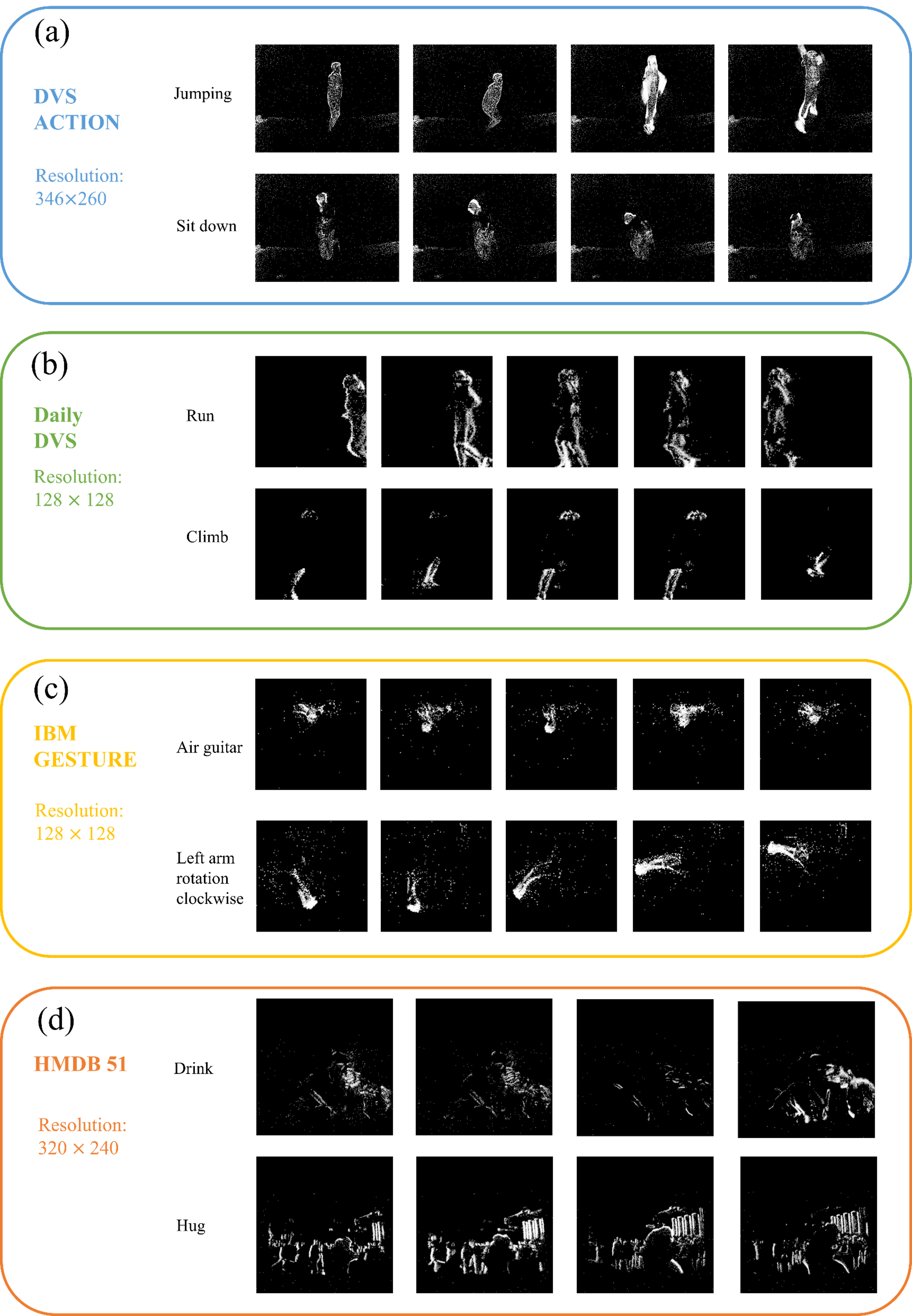
The details of the datasets are shown in Table 9. The DVS 128 Gesture dataset is collected by IBM (Amir et al., 2017), comprising 10/11 gesture classes. It is captured with a DAVIS 128 camera under different lighting conditions with a resolution of 128128. The Daily DVS dataset (Liu et al., 2021a) contains 1440 recordings of 15 subjects performing 12 daily actions under different lighting and camera positions. It is also recorded with DAVIS 128 camera. The DVS Action dataset (Miao et al., 2019) features 10 action classes with 15 subjects performing each action three times. It is recorded with a DAVIS 346 camera with a resolution of 346240. The HMDB51-DVS (Bi et al., 2020) dataset includes 51 human action categories recorded with conventional frame-based camera recordings and subsequently converted into events using DAVIS 240 conversion mode. The resolution is 320240. Each of those datasets has its own application scenario, and all of them are widely used for research and benchmarking in neuromorphic computing. We visualize some samples from the four datasets to understand event-based action recognition better, shown in Fig. 5.
A.5.2 Noise
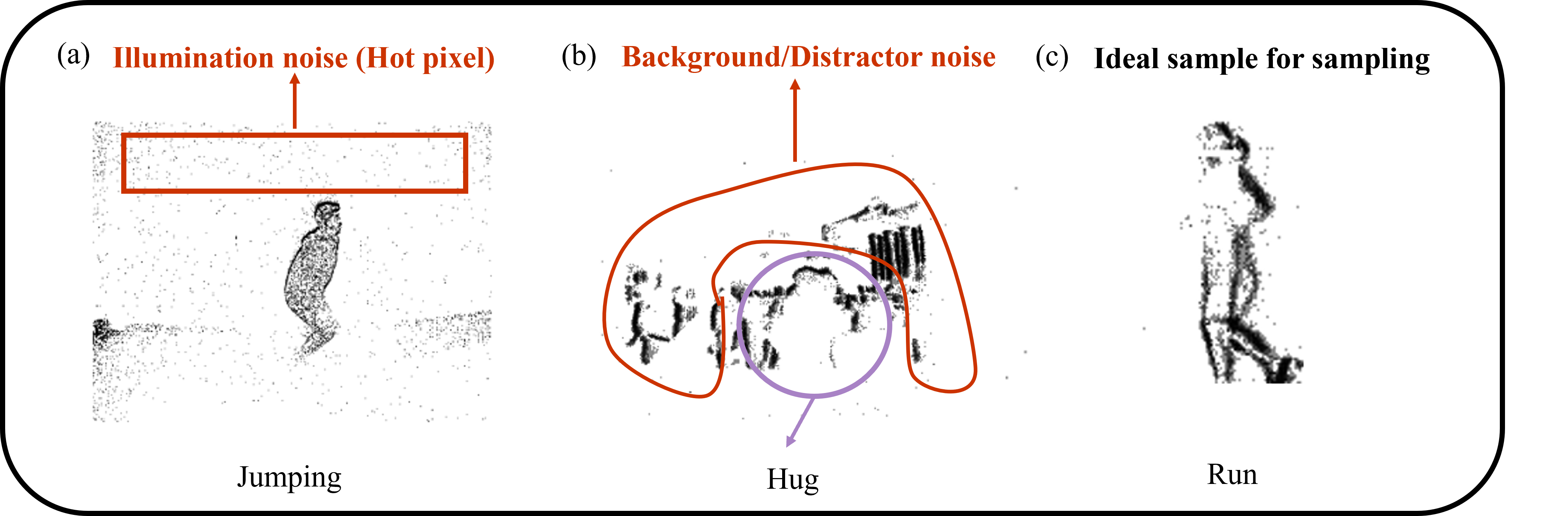
There are two main types of noise in the event data, illumination noise (hot pixels) and background noise. Illumination noise pertains to the noise introduced by changes in ambient lighting conditions during data capture, and background noise is the generated event from the unwanted movement of the background. These two types of noise are represented in all four datasets. For the illumination noise, the DVS Action dataset exhibits noticeable illumination noise, depicted in Fig. 6(a). That noise is likely introduced during the recording, as the illumination noise could be present in certain scenarios. The illumination noise profoundly impairs the effectiveness of the network during random sampling. Consequently, we use the denoising method (Feng et al., 2020) to reduce the noise in the sample and the probability of sampling points from noise. As for the remaining three datasets, their illumination noise is relatively low, so we proceeded directly. As for background noise, HMDB51-DVS indicates a strong presence of background noise. As illustrated in Fig. 6(b), the label is hugging people, and the red area is drawn for the background of the building. Since most of the Point Clouds sent into the network originated from background buildings, the network can not recognize the action. To our best knowledge, this problem remains challenging in the community. The background noise significantly limits the accuracy of the action recognition on the HMDB51-DVS dataset.
A.5.3 Label
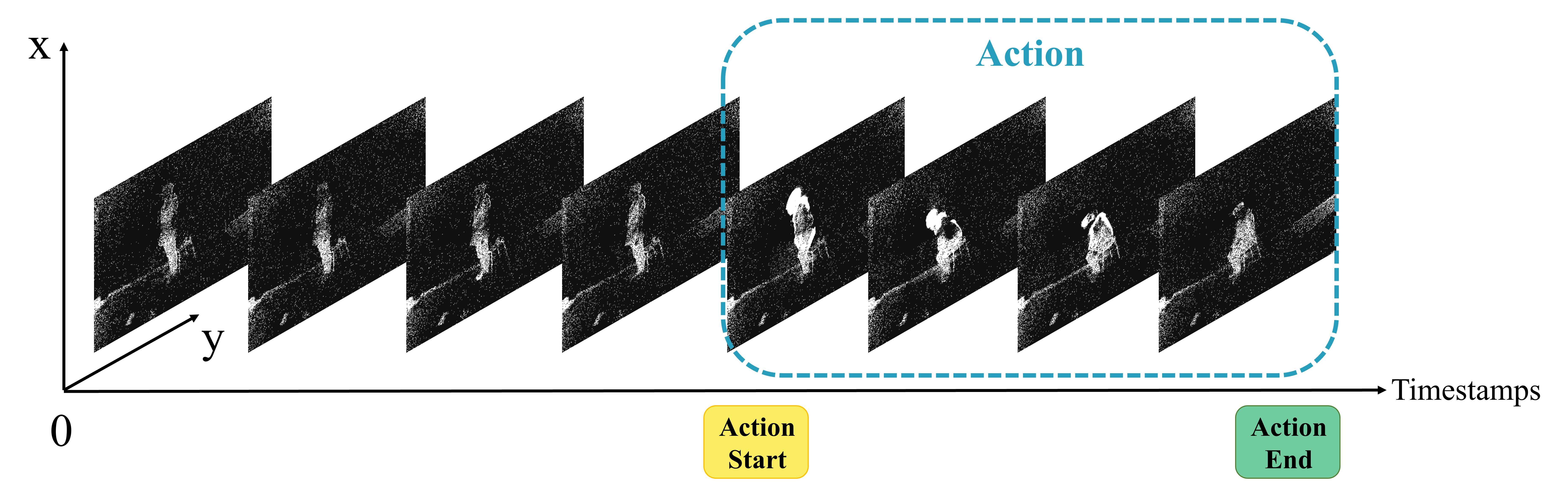
In the DVS Action dataset, there is no detailed timestamp setting, only including the action start and end labels. After we visualize the event stream of the files, as depicted in Fig. 7, we find that almost all actions occur after half of the total dataset. So we set the sampling start point from half of the total timestamps to build the dataset. Compared with the manual annotation method (Wang et al., 2020), our method is straightforward but still achieves better results on the DVS Action dataset.
A.5.4 Sliding window
The appropriate length of the sliding window affects the performance of the network. We initially used a sliding window of 0.5 s in Daily DVS, and the accuracy of the model was only 80% with this setting. After comparative experiments, we finally optimized the value with 1.5 s, representing the average length of the 12 actions identified in the Daily DVS dataset. Determining the appropriate length of the sliding window for describing an action is a valuable task to explore in the future, for instance, an automated adjustment window.
A.6 Overall architecture
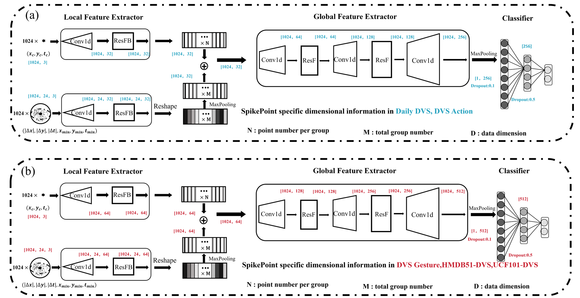
The pipeline which is shown in Fig. 1 begins with the receipt of the original Point Clouds generated by event cameras. A sliding window clip of the original data in the time axis is performed by employing the method discussed in Section 3.1. Subsequently, a random sampling of the Point Clouds in the sliding window is conducted to create a point set of dimensions [, 3]. The sampling and grouping method highlighted in Section 3.2 is then applied to process the set and derive a group set of dimensions [, , 6]. The Point Cloud dimension is subsequently up-dimensioned by employing a multi-local feature extractor, which results in a tensor of dimensions [, , ]. The local features are then reshaped and pooled to obtain a tensor of dimensions [, ], representing the global features. The global features are then extracted utilizing a global feature extractor. The global and local features are abstracted into a single feature vector of dimensions [1, ] by employing the max pooling operation for classification by the classifier.
A.7 Network
A.7.1 Structure
In this work, we keep the same network architecture for all the datasets. Nevertheless, to accommodate datasets of different sizes, the dimensionality of the network in the feature extraction process is adapted. A relatively small network was used for the Daily DVS and DVS Action, and a relatively large network was used for the other two datasets. The details of the small and large networks are highlighted in blue and red in Fig. 8. We use the list to represent the Point Cloud’s dimension change of two different size models, and . The first one represents the change in the dimensionality of the input Point Cloud data by the local feature extractor. The remaining three represent the global feature extractor’s up-dimensioning of the local feature dimension. In addition, the width of the classifier is and in that order. Due to the smaller dimensions output by the global feature extractor compared to other models, the dropout layer is omitted between the extractor and classifier.
A.7.2 LIF or IF
We find that LIF neurons have better performance results on the DVS128 Gesture dataset than IF neurons. They are 98.74% for LIF neurons vs. 97.78% for IF neurons. We speculate that the overfitting of the model is somewhat alleviated due to the leaky of the neurons.
A.7.3 Classifier
The classifier aligns with the majority of network solutions by flattening the features and forwarding them to a spike-based MLP with numerous hidden layers for classification. However, instead of the number of neurons in the last layer being equal to the number of categories, a voting mechanism is used to vote with ten times the spike output. Thus, the number of neurons in the classifier’s last layer is ten times the number of categories for classification. We use mean squared error (MSE) as the loss function of SpikePoint. The equation is as follows:
| (31) |
The model predicts the result as and the actual label as . The encoding timestep of the SNN model is , is the Action recognition category for the dataset, and the loss function is shown above.
A.8 Hyperparameters
We utilize rate encoding to encode coordinates, and the timestep is set to 16. The neuron model we employ is ParamericLIF (Fang et al., 2021b) whose initial is 2.0, and no decay input. In backpropagation, we use the ATan gradient for surrogate training (Neftci et al., 2019).
Our training model uses the following hyperparameters, Batch Size: 6 or 12, Number of Points: 1024, Optimizer: Adam, Initial Learning Rate: , Scheduler: cosine, Max Epochs: 300.