Generalized Neural Sorting Networks with
Error-Free Differentiable Swap Functions

Abstract

Sorting is a fundamental operation of all computer systems, having been a long-standing significant research topic. Beyond the problem formulation of traditional sorting algorithms, we consider sorting problems for more abstract yet expressive inputs, e.g., multi-digit images and image fragments, through a neural sorting network. To learn a mapping from a high-dimensional input to an ordinal variable, the differentiability of sorting networks needs to be guaranteed. In this paper we define a softening error by a differentiable swap function, and develop an error-free swap function that holds non-decreasing and differentiability conditions. Furthermore, a permutation-equivariant Transformer network with multi-head attention is adopted to capture dependency between given inputs and also leverage its model capacity with self-attention. Experiments on diverse sorting benchmarks show that our methods perform better than or comparable to baseline methods.

1 Introduction

Traditional sorting algorithms (Cormen et al., 2022), e.g., bubble sort, insertion sort, and quick sort, are a well-established approach to arranging given instances in computer science. Since such a sorting algorithm is a basic component to build diverse computer systems, it has been a long-standing significant research area in science and engineering, and the sorting networks (Knuth, 1998; Ajtai et al., 1983), which are structurally designed as an abstract device with a fixed number of wires (i.e., a connection for a single swap operation), have been widely used to perform a sorting algorithm on computing hardware.

Given an unordered sequence of $n$ elements $\mathbf{s}=[s_{1},\ldots,s_{n}]\in\mathbb{R}^{n}$, the problem of sorting is defined as to find a permutation matrix $\mathbf{P}\in\{0,1\}^{n\times n}$ that transforms $\mathbf{s}$ into an ordered sequence $\mathbf{s}_{\mathrm{o}}$:

$$\mathbf{s}_{\mathrm{o}}=\mathbf{P}^{\top}\mathbf{s},$$ (1)

where a sorting algorithm is a function $f$ of $\mathbf{s}$ that predicts a permutation matrix $\mathbf{P}$:

$$\mathbf{P}=f(\mathbf{s}).$$ (2)

We generalize the formulation of traditional sorting problems to handle more diverse and expressive types of inputs, e.g., multi-digit images and image fragments, which can contain ordinal information semantically. To this end, we extend the sequence of numbers $\mathbf{s}$ to the sequence of vectors $\mathbf{X}=[\mathbf{x}_{1},\ldots,\mathbf{x}_{n}]^{\top}\in\mathbb{R}^{n\times d}$, where $d\gg 1$ is an input dimensionality, and consider the following:

$$\mathbf{X}_{\mathrm{o}}=\mathbf{P}^{\top}\mathbf{X},$$ (3)

where $\mathbf{X}_{\mathrm{o}}$ and $\mathbf{X}$ are ordered and unordered inputs, respectively. This generalized sorting problem can be reduced to (1) if we are given a proper mapping $g$ from an input $\mathbf{x}\in\mathbb{R}^{d}$ to an ordinal value $s\in\mathbb{R}$. Without such a mapping $g$, predicting $\mathbf{P}$ in (3) remains more challenging than in (1) because $\mathbf{x}$ is often a highly implicative high-dimensional variable. We address this generalized sorting problem by learning a neural sorting network together with mapping $g$ in an end-to-end manner, given training data $\{\mathbf{X}^{(i)},\mathbf{P}_{\mathrm{gt}}^{(i)})\}_{i=1}^{N}$. The main challenge is to make the whole network $f([g(\mathbf{x}_{1}),\ldots,g(\mathbf{x}_{n})])$ with mapping and sorting differentiable to be effectively trained with a gradient-based learning scheme, which is not the case in general. There has been recent research (Grover et al., 2019; Cuturi et al., 2019; Blondel et al., 2020; Petersen et al., 2021; 2022) to tackle the differentiability issue for such a composite function.

In this paper, following a sorting network-based sorting algorithm with differentiable swap functions (DSFs) (Petersen et al., 2021; 2022), we first define a softening error by a sorting network, which indicates a difference between original and smoothed elements. Then, we propose an error-free DSF that resolves an error accumulation problem induced by a soft DSF; this allows us to guarantee a zero error in mapping $\mathbf{X}$ to a proper ordinal value. Based on this, we develop the sorting network with error-free DSFs where we adopt a permutation-equivariant Transformer architecture with multi-head attention (Vaswani et al., 2017) to capture dependency between high-dimensional inputs and also leverage the model capacity of the neural network with a self-attention scheme.

Our contributions can be summarized as follows: (i) We define a softening error that measures a difference between original and smoothed values; (ii) We propose an error-free DSF that resolves the error accumulation problem of conventional DSFs and is still differentiable; (iii) We adopt a permutation-equivariant network with multi-head attention as a mapping from inputs to ordinal variables $g(\mathbf{X})$, unlike $g(\mathbf{x})$; (iv) We demonstrate that our proposed methods are effective in diverse sorting benchmarks, compared to existing baseline methods.

We will make codes publicly available upon publication.

2 Sorting Networks with Differentiable Swap Functions

Following traditional sorting algorithms such as bubble sort, quick sort, and merge sort (Cormen et al., 2022) and sorting networks that are constructed by a fixed number of wires (Knuth, 1998; Ajtai et al., 1983), a swap function is a key ingredient of sorting algorithms and sorting networks:

$$(x^{\prime},y^{\prime})=\mathrm{swap}(x,y),$$ (4)

where $x^{\prime}=\min(x,y)$ and $y^{\prime}=\max(x,y)$, which makes the order of $x$ and $y$ correct. For example, if $x>y$, then $x^{\prime}=y$ and $y^{\prime}=x$. Without loss of generality, we can express $\min(\cdot,\cdot)$ and $\max(\cdot,\cdot)$ to the following equations:

$$\min(x,y)=x\lfloor\sigma(y-x)\rceil+y\lfloor\sigma(x-y)\rceil\quad\textrm{and}\quad\max(x,y)=x\lfloor\sigma(x-y)\rceil+y\lfloor\sigma(y-x)\rceil,$$ (5)

where $\lfloor\cdot\rceil$ rounds to the nearest integer and $\sigma(\cdot)\in[0,1]$ transforms an input to a bounded value, i.e., a probability over inputs. Computing (5) is straightforward, but they are not differentiable. To enable to differentiate a swap function, the soft versions of $\min$ and $\max$ can be defined:

$$\overline{\mathrm{min}}(x,y)=x\sigma(y-x)+y\sigma(x-y)\quad\textrm{and}\quad\overline{\mathrm{max}}(x,y)=x\sigma(x-y)+y\sigma(y-x),$$ (6)

where $\sigma(\cdot)$ is differentiable. In addition to its differentiability, either (5) or (6) can be achieved with a sigmoid function $\sigma(x)$, i.e., a $s$-shaped function, which satisfies the following properties that (i) $\sigma(x)$ is non-decreasing, (ii) $\sigma(x)=1$ if $x\to\infty$, (iii) $\sigma(x)=0$ if $x\to-\infty$, (iv) $\sigma(0)=0.5$, and (v) $\sigma(x)=1-\sigma(-x)$. Also, as discussed by Petersen et al. (2022), the choice of $\sigma$ affects the performance of neural network-based sorting network in theory as well as in practice. For example, an optimal monotonic sigmoid function, visualized in Figure 4, is defined as

$$\sigma_{\mathcal{O}}(x)=\begin{cases}-\frac{1}{16}(\beta x)^{-1}&\textrm{if}\ \beta x<-0.25,\\ 1-\frac{1}{16}(\beta x)^{-1}&\textrm{if}\ \beta x>0.25,\\ \beta x+0.5&\textrm{otherwise},\end{cases}$$ (7)

where $\beta$ is steepness; see the work (Petersen et al., 2022) for the details of these numerical and theoretical analyses. Here, we would like to emphasize that the important point of such monotonic sigmoid functions is strict monotonicity. However, as will be discussed in Section 3, it induces an error accumulation problem, which can degrade the performance of the sorting network.

By either (5) or (6), the permutation matrix $\mathbf{P}$ (henceforth, denoted as $\mathbf{P}_{\mathrm{hard}}$ and $\mathbf{P}_{\mathrm{soft}}$ for (5) and (6), respectively) is calculated by the procedure of sorting network:

1. Building a pre-defined sorting network with a fixed number of wires – a wire is a component for comparing and swapping two elements;

2. Feeding an unordered sequence $\mathbf{s}$ into the pre-defined sorting network and calculating a wire-wise permutation matrix $\mathbf{P}_{i}$ for each wire $i$ iteratively;

3. Calculating the permutation matrix $\mathbf{P}$ by multiplying all wire-wise permutation matrices.

As shown in Figure 5, a set of wires is operated simultaneously, so that each set produces an intermediate permutation matrix $\mathbf{P}_{i}$ at $i$th step. Consequently, $\mathbf{P}^{\top}=\mathbf{P}_{1}^{\top}\mathbf{P}_{2}^{\top}\cdots\mathbf{P}_{k}^{\top}=(\mathbf{P}_{k}\cdots\mathbf{P}_{2}\mathbf{P}_{1})^{\top}$ where $k$ is the number of wire sets, e.g., in Figure 5, $k=5$.

The doubly-stochastic matrix property of $\mathbf{P}$ is shown by the following proposition:

Proposition 1 (Modification of Lemma 3 in the work (Petersen et al., 2022)).

A permutation matrix $\mathbf{P}\in\mathbb{R}^{n\times n}$ is doubly-stochastic, which implies that $\sum_{i=1}^{n}[\mathbf{P}]_{ij}=1$ and $\sum_{j=1}^{n}[\mathbf{P}]_{ij}=1$. In particular, regardless of the definition of a swap function with $\min$, $\max$, $\overline{\mathrm{min}}$, and $\overline{\mathrm{max}}$, hard and soft permutation matrices, i.e., $\mathbf{P}_{\mathrm{hard}}$ and $\mathbf{P}_{\mathrm{soft}}$, are doubly-stochastic.

Proof.

The proof of Proposition 1 is provided in Section D. ∎

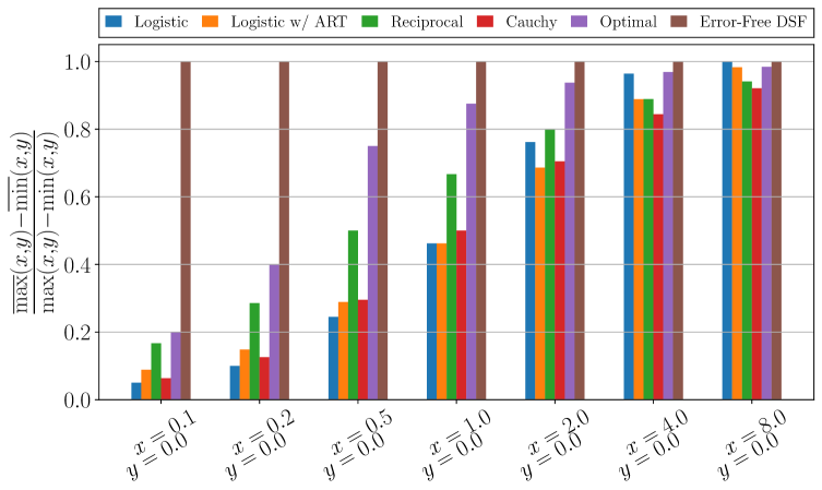
Figure 1: Comparisons of diverse DSFs where a swap function is applied once. After a single operation, two input values $x$ and $y$ are softened while our error-free DSF does not change two values. If a distance between $x$ and $y$ is small, softening is more significant.

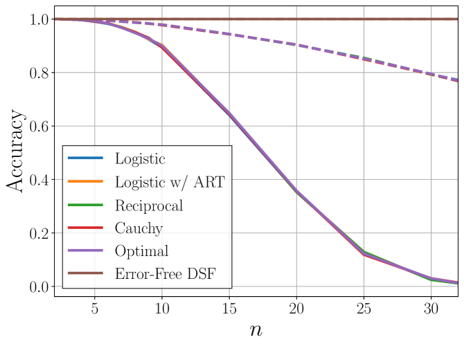
Figure 2: $\mathrm{acc}_{\mathrm{em}}$ (solid) and $\mathrm{acc}_{\mathrm{ew}}$ (dashed), versus sequence lengths. Without a mapping $g$ from $\mathbf{x}$ to $s$, we uniformly sample $n$ elements from $[-10,10]$, which are considered as ordinal scores $\mathbf{s}$. Then, we sort them using the respective sorting networks.

3 Error-Free Differentiable Swap Functions

Before introducing our error-free DSF, we start by describing the motivation of the error-free DSF.

Due to the nature of $\overline{\mathrm{min}}$ and $\overline{\mathrm{max}}$, described in (6), the monotonic DSF changes original input values. For example, if $x<y$, then $x<\overline{\mathrm{min}}(x,y)$ and $\overline{\mathrm{max}}(x,y)<y$ after applying the swap function. It can be a serious problem because a change by the DSF is accumulated as the DSF applies iteratively, called an error accumulation problem in this paper. The results of sigmoid functions such as logistic, logistic with ART, reciprocal, Cauchy, and optimal monotonic functions, and also our error-free DSF are presented in Figure 2, where a swap function is applied once; see the work (Petersen et al., 2022) for the respective sigmoid functions. All DSFs except for our error-free DSF change two values, so that they make two values not distinguishable. In particular, if a difference between two values is small, the consequence of softening is more significant than a case with a large difference. Moreover, if we apply a swap function repeatedly, they eventually become identical; see Figure 6 in Section C. While a swap function is not applied as many as it is tested in the synthetic example, it can still cause the error accumulation problem with a few operations. Here we formally define a softening error, which has been mentioned in this paragraph:

Definition 1.

Suppose that we are given $x$ and $y$ where $x<y$. By (6), these values $x$ and $y$ are softened by a monotonic DSF and they satisfy the following inequalities:

$$x<x^{\prime}=\overline{\mathrm{min}}(x,y)\leq y^{\prime}=\overline{\mathrm{max}}(x,y)<y.$$ (8)

Therefore, we define a difference between the original and the softened values, $x^{\prime}-x$ or $y-y^{\prime}$:

$$y-y^{\prime}=y-\overline{\mathrm{max}}(x,y)=x^{\prime}-x=\overline{\mathrm{min}}(x,y)-x>0,$$ (9)

which is called a softening error in this paper. Without loss of generality, the softening error is $\overline{\mathrm{min}}(x,y)-\min(x,y)$ or $\max(x,y)-\overline{\mathrm{max}}(x,y)$ for any $x,y$.

Note that (9) is satisfied by $y-\overline{\mathrm{max}}(x,y)=y(1-\sigma(y-x))-x\sigma(x-y)=y\sigma(x-y)-x(1-\sigma(y-x))=\overline{\mathrm{min}}(x,y)-x$, using (6) and $\sigma(x-y)=1-\sigma(y-x)$.

With Definition 1, we are able to specify the seriousness of the error accumulation problem:

Proposition 2.

Suppose that $x$ and $y$ are given and a DSF is applied $k$ times. Assuming an extreme scenario that $k\to\infty$, error accumulation becomes $(\max(x,y)-\min(x,y))/2$, under the assumption that $\nabla_{x}\sigma(x)>0$.

Proof.

The proof of this proposition can be found in Section E. ∎

As mentioned in the proof of Proposition 2 and empirically shown in Figure 2, a swap function with relatively large $\nabla_{x}\sigma(x)$ changes the original values $x,y$ significantly compared to a swap function with relatively small $\nabla_{x}\sigma(x)$ – they tend to become identical with a small number of operations in the case of large $\nabla_{x}\sigma(x)$.

In addition to the error accumulation problem, such a DSF depends on the scale of $x-y$ as shown in Figure 2. If $x<y$ but $x$ and $y$ are close enough, $\sigma(y-x)$ is between $0.5$ to $1$, which implies that the error can be induced by the scale of $x-y$ (or $y-x$) as well.

To tackle the aforementioned problem of error accumulation, we propose an error-free DSF:

$$(x^{\prime},y^{\prime})=\mathrm{swap}_{\mathrm{error}\textrm{-}\mathrm{free}}(x,y),$$ (10)

where

$$x^{\prime}=\left(\min(x,y)-\overline{\mathrm{min}}(x,y)\right)_{\mathrm{sg}}+\overline{\mathrm{min}}(x,y)\quad\textrm{and}\quad y^{\prime}=\left(\max(x,y)-\overline{\mathrm{max}}(x,y)\right)_{\mathrm{sg}}+\overline{\mathrm{max}}(x,y).$$ (11)

Note that $\mathrm{sg}$ indicates that gradients are stopped amid backward propagation, inspired by a straight-through estimator (Bengio et al., 2013). At a step for forward propagation, the error-free DSF produces $x^{\prime}=\min(x,y)$ and $y^{\prime}=\max(x,y)$. On the contrary, at a step for backward propagation, the gradients of $\overline{\mathrm{min}}$ and $\overline{\mathrm{max}}$ are used to update learnable parameters. Consequently, our error-free DSF does not smooth the original elements as shown in Figure 2 and ours shows the 100% accuracy for $\mathrm{acc}_{\mathrm{em}}$ and $\mathrm{acc}_{\mathrm{ew}}$ (see Section 5 for their definitions) as shown in Figure 2. Compared to our DSF, existing DSFs do not correspond the original elements to the elements that have been compared and fail to achieve reasonable performance as a sequence length increases, in the cases of Figure 2.

By (5), (6), and (11), we obtain the following:

$$x^{\prime} =\left((x\lfloor\sigma_{yx}\rceil+y\lfloor\sigma_{xy}\rceil)-(x\sigma_{yx}+y\sigma_{xy})\right)_{\mathrm{sg}}+(x\sigma_{yx}+y\sigma_{xy})$$

$$=x\left((\lfloor\sigma_{yx}\rceil-\sigma_{yx})_{\mathrm{sg}}+\sigma_{yx}\right)+y\left((\lfloor\sigma_{xy}\rceil-\sigma_{xy})_{\mathrm{sg}}+\sigma_{xy}\right),$$ (12)

$$y^{\prime} =x\left((\lfloor\sigma_{xy}\rceil-\sigma_{xy})_{\mathrm{sg}}+\sigma_{xy}\right)+y\left((\lfloor\sigma_{yx}\rceil-\sigma_{yx})_{\mathrm{sg}}+\sigma_{yx}\right),$$ (13)

which can be used to define a permutation matrix with the error-free DSF, where $\sigma_{xy}$ and $\sigma_{yx}$ are $\sigma(x-y)$ and $\sigma(y-x)$, respectively. For example, if $n=2$, a permutation matrix $\mathbf{P}$ over $[x,y]$ is

$$\mathbf{P}=\left[\begin{matrix}(\lfloor\sigma_{yx}\rceil-\sigma_{yx})_{\mathrm{sg}}+\sigma_{yx}&(\lfloor\sigma_{xy}\rceil-\sigma_{xy})_{\mathrm{sg}}+\sigma_{xy}\\ (\lfloor\sigma_{xy}\rceil-\sigma_{xy})_{\mathrm{sg}}+\sigma_{xy}&(\lfloor\sigma_{yx}\rceil-\sigma_{yx})_{\mathrm{sg}}+\sigma_{yx}\\ \end{matrix}\right].$$ (14)

To sum up, we can describe the following proposition on our error-free DSF, $\mathrm{swap}_{\mathrm{error}\textrm{-}\mathrm{free}}(\cdot,\cdot)$:

Proposition 3.

By (11), the softening error $x^{\prime}-\min(x,y)$ (or $\max(x,y)-y^{\prime}$) for an error-free DSF is zero.

Proof.

The proof of this proposition is presented in Section F. ∎

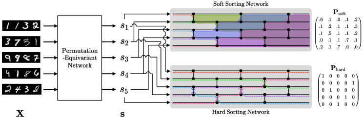
Figure 3: Illustration of our neural sorting network with error-free DSFs. Given high-dimensional inputs $\mathbf{X}$, a permutation-equivariant network produces a vector of ordinal variables $\mathbf{s}$, which is used to be swapped using soft or hard sorting network.

4 Neural Sorting Networks with Error-Free Differentiable Swap Functions

In this section we build a generalized neural network-based sorting network with the error-free DSF and a permutation-equivariant neural network, considering the properties covered in Section 3.

First, we describe a procedure for transforming a high-dimensional input to an ordinal score. Such a mapping $g:\mathbb{R}^{d}\to\mathbb{R}$, which consists of a set of learnable parameters, has to satisfy a permutation-equivariant property:

$$[g(\mathbf{x}_{\pi_{1}}),\ldots,g(\mathbf{x}_{\pi_{n}})]=\pi([g(\mathbf{x}_{1}),\ldots,g(\mathbf{x}_{n})]),$$ (15)

where $\pi_{i}=[\pi([1,\ldots,n])]_{i}\ \forall i\in[n]$, for any permutation function $\pi$. Typically, an instance-wise neural network, which is applied to each element in a sequence given, is permutation-equivariant (Zaheer et al., 2017). Based on this consequence, instance-wise CNNs are employed in differentiable sorting algorithms (Grover et al., 2019; Cuturi et al., 2019; Petersen et al., 2021; 2022). However, such an instance-wise architecture is limited since it is ineffective for capturing essential features from a sequence. Some types of neural networks such as long short-term memory (Hochreiter & Schmidhuber, 1997) and the standard Transformer architecture (Vaswani et al., 2017) are capable of modeling a sequence of instances, utilizing recurrent connections, scaled dot-product attention, or parameter sharing across elements. While they are powerful for modeling a sequence, they are not obviously permutation-equivariant. Unlike such permutation-variant models, we propose a robust Transformer-based network that satisfies the permutation-equivariant property, which is inspired by the recent work (Vaswani et al., 2017; Lee et al., 2019).

To present our network, we briefly introduce a scaled dot-product attention and multi-head attention:

$$\mathrm{att}(\mathbf{Q},\mathbf{K},\mathbf{V})=\mathrm{softmax}\left(\frac{\mathbf{Q}\mathbf{K}^{\top}}{\sqrt{d_{m}}}\right)\mathbf{V}\quad\textrm{and}\quad\mathrm{mha}(\mathbf{Q},\mathbf{K},\mathbf{V})=[\mathrm{head}_{1},\ldots,\mathrm{head}_{h}]\mathbf{W}_{o},$$ (16)

where $\mathrm{head}_{i}=\mathrm{att}(\mathbf{Q}\mathbf{W}_{q}^{(i)},\mathbf{K}\mathbf{W}_{k}^{(i)},\mathbf{V}\mathbf{W}_{v}^{(i)})$, $\mathbf{Q},\mathbf{K},\mathbf{V}\!\in\!\mathbb{R}^{n\times hd_{m}}$, $\mathbf{W}_{q}^{(i)},\mathbf{W}_{k}^{(i)},\mathbf{W}_{v}^{(i)}\!\in\!\mathbb{R}^{hd_{m}\times d_{m}}$, and $\mathbf{W}_{o}\!\in\!\mathbb{R}^{hd_{m}\times hd_{m}}$. Similar to the Transformer network, a series of $\mathrm{mha}$ blocks is stacked with layer normalization (Ba et al., 2016) and residual connections (He et al., 2016), and in this paper $\mathbf{X}$ is processed by $\mathrm{mha}(\mathbf{Z},\mathbf{Z},\mathbf{Z})$ where $\mathbf{Z}=g^{\prime}(\mathbf{X})$ or $\mathbf{Z}$ is the output of previous layer; see Section H for the details of the architectures. Note that $g^{\prime}(\cdot)$ is an instance-wise embedding layer, e.g., a simple fully-connected network or a simple CNN. Importantly, compared to the standard Transformer model, our network does not include a positional embedding, in order to satisfy the permutation-equivariant property; $\mathrm{mha}(\mathbf{Z},\mathbf{Z},\mathbf{Z})$ satisfies (15) for the permutation of $\mathbf{z}_{1},\ldots,\mathbf{z}_{n}$ where $\mathbf{Z}=[\mathbf{z}_{1},\ldots,\mathbf{z}_{n}]^{\top}$. The output of our network is $\mathbf{s}$, followed by the last instance-wise fully-connected layer. Finally, as shown in Figure 3, our sorting network is able to produce differentiable permutation matrices over $\mathbf{s}$, i.e., $\mathbf{P}_{\mathrm{hard}}$ and $\mathbf{P}_{\mathrm{soft}}$, by utilizing (11) and (6), respectively. Note that $\mathbf{P}_{\mathrm{hard}}$ and $\mathbf{P}_{\mathrm{soft}}$ are doubly-stochastic by Proposition 1.

To learn the permutation-equivariant network $g$, we define both objectives for $\mathbf{P}_{\mathrm{soft}}$ and $\mathbf{P}_{\mathrm{hard}}$:

$$\mathcal{L}_{\mathrm{soft}} =-\sum_{i=1}^{n}\sum_{j=1}^{n}[\mathbf{P}_{\mathrm{gt}}\log\mathbf{P}_{\mathrm{soft}}+(1-\mathbf{P}_{\mathrm{gt}})\log(1-\mathbf{P}_{\mathrm{soft}})]_{ij},$$ (17)

$$\mathcal{L}_{\mathrm{hard}} =\|\mathbf{X}_{\mathrm{o},\mathrm{hard}}-\mathbf{X}_{\mathrm{o},\mathrm{gt}}\|_{F}^{2}=\|\mathbf{P}_{\mathrm{hard}}^{\top}\mathbf{X}-\mathbf{P}_{\mathrm{gt}}^{\top}\mathbf{X}\|_{F}^{2},$$ (18)

where $\mathbf{P}_{\mathrm{gt}}$ is a ground-truth permutation matrix. Note that all the operations in $\mathcal{L}_{\mathrm{soft}}$ are entry-wise. Similar to (17), the objective (18) for $\mathbf{P}_{\mathrm{hard}}$ might be designed as the form of binary cross-entropy, which tends to be generally robust in training deep neural networks. However, we struggle to apply the binary cross-entropy for $\mathbf{P}_{\mathrm{hard}}$ into our problem formulation, due to discretized loss values. In particular, the form of cross-entropy for $\mathbf{P}_{\mathrm{hard}}$ can be used to train the sorting network, but degrades its performance in our preliminary experiments. Thus, we design the objective for $\mathbf{P}_{\mathrm{hard}}$ as $\mathcal{L}_{\mathrm{hard}}=\|\mathbf{X}_{\mathrm{o},\mathrm{hard}}-\mathbf{X}_{\mathrm{o},\mathrm{gt}}\|_{F}^{2}$ with the Frobenius norm, which helps to train the network more robustly.

In addition, using a proposition on splitting $\mathbf{P}_{\mathrm{hard}}$, which is discussed in Section G, the objective (18) for $\mathbf{P}_{\mathrm{hard}}$ can be modified by splitting $\mathbf{P}_{\mathrm{hard}}$, $\mathbf{P}_{\mathrm{gt}}$, and $\mathbf{X}$, which is able to reduce the number of possible permutations; see the associated section for the details. Eventually, our network $g$ is trained by the combined loss $\mathcal{L}=\mathcal{L}_{\mathrm{soft}}+\lambda\mathcal{L}_{\mathrm{hard}}$ where $\lambda$ is a balancing hyperparameter; analysis on $\lambda$ can be found in the appendices. As mentioned above, a landscape of $\mathcal{L}_{\mathrm{hard}}$ is not smooth due to the property of straight-through estimator, even though we use $\mathcal{L}_{\mathrm{hard}}$. Thus, we combine both objectives to the form of a single loss, which is widely adopted in a deep learning community.

5 Experimental Results

We demonstrate experimental results to show the validity of our methods. Our neural network-based sorting network aims to solve two benchmarks: sorting (i) multi-digit images and (ii) image fragments. Unless otherwise specified, an odd-even sorting network is used in the experiments. We measure the performance of each method in $\mathrm{acc}_{\mathrm{em}}$ and $\mathrm{acc}_{\mathrm{ew}}$:

$$\mathrm{acc}_{\mathrm{em}}=\frac{\sum_{i=1}^{N}\bigcap_{j=1}^{n}{\boldsymbol{1}}\big{(}\left[\hat{\mathbf{s}}^{(i)}\right]_{j}=\left[\tilde{\mathbf{s}}^{(i)}\right]_{j}\big{)}}{N}\quad\textrm{and}\quad\mathrm{acc}_{\mathrm{ew}}=\frac{\sum_{i=1}^{N}\sum_{j=1}^{n}{\boldsymbol{1}}\big{(}\left[\hat{\mathbf{s}}^{(i)}\right]_{j}=\left[\tilde{\mathbf{s}}^{(i)}\right]_{j}\big{)}}{Nn},$$ (19)

where $\mathrm{argsort}$ returns the indices to sort a given vector and $\boldsymbol{1}(\cdot)$ is an indicator function. Note that

$$\hat{\mathbf{s}}^{(i)}=\mathrm{argsort}\left(\mathbf{P}^{(i)\top}_{\mathrm{gt}}\mathbf{s}^{(i)}\right)\quad\textrm{and}\quad\tilde{\mathbf{s}}^{(i)}=\mathrm{argsort}\left(\mathbf{P}^{(i)\top}\mathbf{s}^{(i)}\right).$$ (20)

We attempt to match the capacities of the Transformer-based models to the conventional CNNs. As described in Tables 1, 2, and 3, the capacities of the small Transformer-based models are smaller than or similar to the capacities of the CNNs in terms of FLOPs and the number of parameters.

5.1 Sorting Multi-Digit Images

Table 1: Results on sorting the four-digit MNIST dataset. The results are measured in $\mathrm{acc}_{\mathrm{em}}$ and $\mathrm{acc}_{\mathrm{ew}}$ (in parentheses). FLOPs is on the basis of a sequence length 3. All the values are averaged over 5 runs with different seeds.

Method		Model	Sequence Length						FLOPs	#Param.
			3	5	7	9	15	32
NeuralSort		CNN	91.9 (94.5)	77.7 (90.1)	61.0 (86.2)	43.4 (82.4)	9.7 (71.6)	0.0 (38.8)	130M	855K
Sinkhorn Sort			92.8 (95.0)	81.1 (91.7)	65.6 (88.2)	49.7 (84.7)	12.6 (74.2)	0.0 (41.2)
Fast Sort & Rank			90.6 (93.5)	71.5 (87.2)	49.7 (81.3)	29.0 (75.2)	2.8 (60.9)	–
Diffsort	Logistic		92.0 (94.5)	77.2 (89.8)	54.8 (83.6)	37.2 (79.4)	4.7 (62.3)	0.0 (56.3)
	Logistic w/ ART		94.3 (96.1)	83.4 (92.6)	71.6 (90.0)	56.3 (86.7)	23.5 (79.4)	0.5 (64.9)
	Reciprocal		94.4 (96.1)	85.0 (93.3)	73.4 (90.7)	60.8 (88.1)	30.2 (81.9)	1.0 (66.8)
	Cauchy		94.2 (96.0)	84.9 (93.2)	73.3 (90.5)	63.8 (89.1)	31.1 (82.2)	0.8 (63.3)
	Optimal		94.6 (96.3)	85.0 (93.3)	73.6 (90.7)	62.2 (88.5)	31.8 (82.3)	1.4 (67.9)
Ours	Error-Free DSFs	CNN	94.8 (96.4)	86.9 (94.1)	74.2 (90.9)	62.6 (88.6)	34.7 (83.3)	2.1 (69.2)	130M	855K
		Transformer-S	95.9 (97.1)	94.8 (97.5)	90.8 (96.5)	86.9 (95.7)	74.3 (93.6)	37.8 (87.7)	130M	665K
		Transformer-L	96.5 (97.5)	95.4 (97.7)	92.9 (97.2)	90.1 (96.5)	82.5 (95.0)	46.2 (88.9)	137M	3.104M

Table 2: Results on sorting the SVHN dataset. FLOPs is computed on the basis of a sequence length 3. All the values are averaged over 5 runs with different seeds.

Method		Model	Sequence Length					FLOPs	#Param.
			3	5	7	9	15
Diffsort	Logistic	CNN	76.3 (83.2)	46.0 (72.7)	21.8 (63.9)	13.5 (61.7)	0.3 (45.9)	326M	1.226M
	Logistic w/ ART		83.2 (88.1)	64.1 (82.1)	43.8 (76.5)	24.2 (69.6)	2.4 (56.8)
	Reciprocal		85.7 (89.8)	68.8 (84.2)	53.3 (80.0)	40.0 (76.3)	13.2 (66.0)
	Cauchy		85.5 (89.6)	68.5 (84.1)	52.9 (79.8)	39.9 (75.8)	13.7 (66.0)
	Optimal		86.0 (90.0)	67.5 (83.5)	53.1 (80.0)	39.1 (76.0)	13.2 (66.3)
Ours	Error-Free DSFs	CNN	86.8 (90.6)	68.9 (84.5)	53.4 (80.4)	40.0 (77.0)	12.0 (65.3)	326M	1.226M
		Transformer-S	86.6 (90.2)	72.6 (85.7)	62.5 (83.5)	48.6 (79.3)	19.3 (69.6)	210M	1.223M
		Transformer-L	88.0 (91.2)	74.0 (86.3)	63.9 (83.8)	50.2 (80.1)	21.7 (71.2)	332M	3.475M

Datasets.

As steadily utilized in the previous work (Grover et al., 2019; Cuturi et al., 2019; Blondel et al., 2020; Petersen et al., 2021; 2022), we create a four-digit dataset by concatenating four images from the MNIST dataset (LeCun et al., 1998); see Figure 3 for some examples of the dataset. On the other hand, the SVHN dataset (Netzer et al., 2011) contains multi-digit numbers extracted from street view images and is therefore suitable for sorting.

Experimental Details.

We conduct the experiments 5 times by varying random seeds to report the average of $\mathrm{acc}_{\mathrm{em}}$ and $\mathrm{acc}_{\mathrm{ew}}$, and use an optimal monotonic sigmoid function as DSFs. The performance of each model is measured by a test dataset. We use the AdamW optimizer (Loshchilov & Hutter, 2018), and train each model for 200,000 steps on the four-digit MNIST dataset and 300,000 steps on the SVHN dataset. Unless otherwise noted, we follow the same settings of the work (Petersen et al., 2022) for fair comparisons. The missing details are described in Section I.

Results.

Tables 1 and 2 show the results of the previous work such as NeuralSort (Grover et al., 2019), Sinkhorn Sort (Cuturi et al., 2019), Fast Sort & Rank (Blondel et al., 2020), and Diffsort (Petersen et al., 2021; 2022), and our methods on the MNIST and SVHN datasets, respectively. When we use the conventional CNN as a permutation-equivariant network, our method shows better than or comparable to the previous methods. As we exploit more powerful models, i.e., small and large Transformer-based permutation-equivariant models, our approaches show better results compared to other existing methods including our method with the conventional CNN.

5.2 Sorting Image Fragments

Table 3: Results on sorting image fragments of MNIST and CIFAR-10. 2 $\times$ 2 and 3 $\times$ 3 indicate the number of fragments, and 14 $\times$ 14, 9 $\times$ 9, 16 $\times$ 16, and 10 $\times$ 10 (in parentheses) indicate the size of image fragments. FLOPs is computed on the basis of the MNIST 2 $\times$ 2 (14 $\times$ 14) case and the CIFAR-10 2 $\times$ 2 (16 $\times$ 16) case. All the values are averaged over 5 runs with different seeds.

Method		Model	MNIST				CIFAR-10
			2 $\times$ 2	3 $\times$ 3	FLOPs	#Param.	2 $\times$ 2	3 $\times$ 3	FLOPs	#Param.
			(14 $\times$ 14)	(9 $\times$ 9)			(16 $\times$ 16)	(10 $\times$ 10)
Diffsort	Logistic	CNN	98.5 (99.0)	5.3 (42.9)	1.498M	84K	56.9 (73.6)	0.8 (27.7)	1.663M	85K
	Logistic w/ ART		98.4 (99.1)	5.4 (42.9)			56.7 (73.4)	0.7 (27.7)
	Reciprocal		98.4 (99.2)	5.3 (42.9)			56.7 (73.4)	0.7 (27.8)
	Cauchy		98.4 (99.2)	5.3 (42.9)			56.9 (73.6)	0.9 (27.9)
	Optimal		98.4 (99.1)	5.3 (43.0)			56.6 (73.4)	0.7 (27.7)
Ours	Error-Free DSFs	CNN	98.4 (99.2)	5.2 (42.6)	1.498M	84K	56.9 (73.6)	0.8 (28.0)	1.663M	85K
		Transformer	98.6 (99.2)	5.6 (43.7)	946K	87K	58.1 (74.2)	0.9 (28.3)	1.111M	87K

Datasets.

When inputs are fragments, we use two datasets: the MNIST dataset (LeCun et al., 1998) and the CIFAR-10 dataset (Krizhevsky & Hinton, 2009). Similar to the work (Mena et al., 2018), we create multiple fragments (or patches) from a single-digit image of the MNIST dataset to utilize themselves as inputs – for example, 4 fragments of size 14 $\times$ 14 or 9 fragments of size 9 $\times$ 9 are created from a single image. Similarly, the CIFAR-10 dataset, which contains various objects, e.g., birds and cats, is split to multiple patches, and then is used to the experiments on sorting image fragments. See Table 3 for the details of the fragments.

Experimental Details.

Similar to the experiments on sorting multi-digit images, an optimal monotonic sigmoid function is used as DSFs. Since the size of inputs is much smaller than the experiments on sorting multi-digit images, shown in Section 5.1, we modify the architectures of the CNNs and the Transformer-based models. We reduce the kernel size of convolution layers from five to three and make strides two. Due to the small input size, we omit the results by a large Transformer-based model for these experiments. Additionally, max-pooling operations are removed. Similar to the experiments in Section 5.1, we use the AdamW optimizer (Loshchilov & Hutter, 2018). Moreover, each model is trained for 50,000 steps when the number of fragments is $2\times 2$, i.e., when a sequence length is 4, and 100,000 steps for $3\times 3$ fragments, i.e., when a sequence length is 9. Additional information including the details of neural architectures can be found in the appendices.

Results.

Table 3 represents the experimental results on both datasets of image fragments, which are created from the MNIST and CIFAR-10 datasets. Similar to the experiments on sorting multi-digit images, the more powerful architecture improves performance in this task.

According to the experimental results, we achieve satisfactory performance by applying error-free DSFs, combined loss, and Transformer-based models with multi-head attention. We provide detailed discussion on how they contribute to the performance gain in Section 7, and empirical studies on steepness, learning rate, and a balancing hyperparameter in Section 7 and the appendices.

6 Related Work

Differentiable Sorting Algorithms.

To allow us to differentiate a sorting algorithm, Grover et al. (2019) have proposed the continuous relaxation of $\mathrm{argsort}$ operator, which is named NeuralSort. In this work the output of NeuralSort only satisfies the row-stochastic matrix property, although Grover et al. (2019) attempt to employ a gradient-based optimization strategy in learning a neural sorting algorithm. Cuturi et al. (2019) propose the smoothed ranking and sorting operators using optimal transport, which is the natural relaxation for assignments. To reduce the cost of the optimal transport, the Sinkhorn algorithm (Cuturi, 2013) is used. Then, the reference (Blondel et al., 2020) has proposed the first differentiable sorting and ranking operators with $\mathcal{O}(n\log n)$ time and $\mathcal{O}(n)$ space complexities, which is named Fast Rank & Sort, by constructing differentiable operators as projections on permutahedron. The work (Petersen et al., 2021) has suggested a differentiable sorting network with relaxed conditional swap functions. Recently, the same authors analyze the characteristics of the relaxation of monotonic conditional swap functions, and propose several monotonic swap functions, e.g., Cauchy and optimal monotonic functions (Petersen et al., 2022).

Permutation-Equivariant Networks.

A seminal architecture, long short-term memory (Hochreiter & Schmidhuber, 1997) can be used in modeling a sequence without any difficulty, and a sequence-to-sequence model (Sutskever et al., 2014) can be employed to cope with a sequence. However, as discussed in the work (Vinyals et al., 2016), an unordered sequence can have good orderings, by analyzing the effects of permutation thoroughly. Zaheer et al. (2017) propose a permutation-invariant or permutation-equivariant network, named Deep Sets, and prove the permutation invariance and permutation equivariance of the proposed models. By utilizing a Transformer network (Vaswani et al., 2017), Lee et al. (2019) propose a permutation-equivariant network.

7 Discussion

Numerical Analysis on Our Methods and Their Hyperparameters.

Table 4: Study on comparisons of Diffsort with an optimal monotonic sigmoid function and our methods in the experiments of sorting the four-digit MNIST dataset

Method	Model	Sequence Length
		3	5	7	9	15	32
Diffsort	CNN	94.6 (96.3)	85.0 (93.3)	73.6 (90.7)	62.2 (88.5)	31.8 (82.3)	1.4 (67.9)
Ours		94.8 (96.4)	86.9 (94.1)	74.2 (90.9)	62.6 (88.6)	34.7 (83.3)	2.1 (69.2)
Diffsort	Transformer-S	95.9 (97.1)	90.2 (95.4)	83.9 (94.2)	77.2 (92.9)	57.3 (89.7)	16.3 (81.7)
Ours		95.9 (97.1)	94.8 (97.5)	90.8 (96.5)	86.9 (95.7)	74.3 (93.6)	37.8 (87.7)
Diffsort	Transformer-L	96.5 (97.5)	92.6 (96.4)	87.6 (95.3)	82.6 (94.3)	67.8 (92.0)	32.1 (85.7)
Ours		96.5 (97.5)	95.4 (97.7)	92.9 (97.2)	90.1 (96.5)	82.5 (95.0)	46.2 (88.9)

We carry out a numerical analysis on the effects of our methods, compared to a baseline method, i.e., Diffsort with an optimal monotonic sigmoid function. As presented in Table 4, we demonstrate that our methods better sorting performance compared to the baseline, which implies that our suggestions are effective in the sorting tasks. In these experiments, we follow the settings of the experiments described in Section 5.1. Moreover, we demonstrate numerical analyses on a balancing hyperparameter, steepness, and learning rate in the appendices.

Analysis on Performance Gains.

According to the results in Sections 5 and 7, we can argue that error-free DSFs, our proposed loss, and Transformer-based models contribute to better performance appropriately compared to the baseline methods. As shown in Tables 1 and 4, the performance gains by Transformer-based models are more substantial than the gains by error-free DSFs and our loss, since multi-head attention is effective for capturing long-term dependency (or dependency between multiple instances in our case) and reducing inductive biases. However, as will be discussed in the following, the hard permutation matrices can be used in the case that does not allow us to mix instances in $\mathbf{X}$, e.g., sorting image fragments in Section 5.2.

Utilization of Hard Permutation Matrices.

While a soft permutation matrix $\mathbf{P}_{\mathrm{soft}}$ is limited to be utilized itself directly, a hard permutation matrix $\mathbf{P}_{\mathrm{hard}}$ is capable of being applied in a case that requires $\mathbf{P}_{\mathrm{hard}}$; each row of $\mathbf{P}_{\mathrm{soft}}^{\top}\mathbf{X}$ is a linear combination of some column of $\mathbf{P}_{\mathrm{soft}}$ and $\mathbf{X}$, but one of $\mathbf{P}_{\mathrm{hard}}^{\top}\mathbf{X}$ corresponds to an exact row in $\mathbf{X}$. The experiments in Section 5.2 are one of such cases, and it exhibits our strength, not only the performance in $\mathrm{acc}_{\mathrm{em}}$ and $\mathrm{acc}_{\mathrm{ew}}$.

Effects of Multi-Head Attention in the Problem (3).

We follow the model architecture, which is used in the previous work (Grover et al., 2019; Cuturi et al., 2019; Petersen et al., 2021; 2022), for the CNNs. However, as shown in Tables 1, 2, and 3, the model is not enough to show the best performance. In particular, whereas the model capacity, i.e., FLOPs and the number of parameters, of the small Transformer models is almost matched to or less than the capacity of the CNNs, the results by the small Transformer models outperform the results by the CNNs. We presume that these performance gains are derived from a multi-head attention’s ability to capture long-term dependency and reduce an inductive bias, as widely stated in many recent studies in diverse fields such as natural language processing (Vaswani et al., 2017; Devlin et al., 2018; Brown et al., 2020), computer vision (Dosovitskiy et al., 2021; Liu et al., 2021), and 3D vision (Nash et al., 2020; Zhao et al., 2021). Especially, unlike the instance-wise CNNs, our permutation-equivariant Transformer architecture utilizes self-attention given instances, so that our model can productively compare instances in a sequence and effectively learn the relative relationship between them.

Further Study of Differentiable Sorting Algorithms.

Differentiable sorting encourages us to train a mapping from an abstract input to an ordinal score using supervision on permutation matrices. However, this line of studies is limited to a sorting problem of high-dimensional data with clear ordering information, e.g., multi-digit numbers. As the further study of differentiable sorting, we can expand this framework to sort more ambiguous data, which contains implicitly ordinal information.

8 Conclusion

In this paper, we defined a softening error, induced by a monotonic DSF, and demonstrated several evidences of the error accumulation problem. To resolve the error accumulation problem, an error-free DSF is proposed, inspired by a straight-through estimator. Moreover, we provided the simple theoretical and empirical analyses that our error-free DSF successfully achieves a zero error and also holds non-decreasing and differentiability conditions. By combining all components, we suggested a generalized neural sorting network with the error-free DSF using multi-head attention. Finally we showed that our methods are better than or comparable to other algorithms in diverse benchmarks.

Appendix A Optimal Monotonic Sigmoid Function

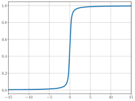
Figure 4: An optimal monotonic sigmoid function, shown in (7)

We visualize an optimal monotonic sigmoid function in Figure 4.

Appendix B Visualization of Sorting Network

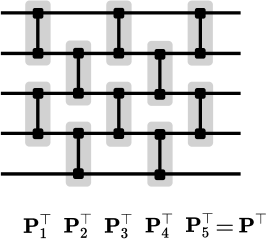
Figure 5: A sorting network with 5 wire sets

Figure 5 shows an example of a sorting network and permutation matrices.

Appendix C Comparisons of Differentiable Swap Functions

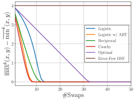
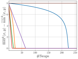
Figure 6: Comparisons of diverse DSFs in terms of how many times a swap function is conducted. Our error-free DSF does not change the original $x$ and $y$, compared to other DSFs. We set (left) $x=4,y=0$ or (right) $x=8,y=0$ initially. We conduct a swap functions $k$ times where $k=\#\textrm{Swaps}$.

As shown in Figure 6, some sigmoid functions, i.e., logistic, logistic with ART, reciprocal, Cauchy, and optimal monotonic functions suffer from the error accumulation problem; see the work (Petersen et al., 2022) for the details of such sigmoid functions. For the case of the Cauchy function, two values are close enough at $9$th step in the left panel of Figure 6 and $15$th step in the right panel of Figure 6; we present the corresponding step where a difference between two values becomes smaller than 0.001.

Appendix D Proof of Proposition 1

Proof.

If two elements at indices $i$ and $j$ are swapped by a single swap function, $[\mathbf{P}]_{kk}=1$ for $k\in[n]\backslash\{i,j\}$, $[\mathbf{P}]_{kl}=0$ for $k\neq l$, $k,l\in[n]\backslash\{i,j\}$, $[\mathbf{P}]_{ii}=[\mathbf{P}]_{jj}=p$, and $[\mathbf{P}]_{ij}=[\mathbf{P}]_{ji}=1-p$, where $p$ is the output of sigmoid function, i.e., $p=\sigma(y-x)$ or $p=\lfloor\sigma(y-x)\rceil$. Since the multiplication of doubly-stochastic matrices is still doubly-stochastic, Proposition 1 is true. ∎

Appendix E Proof of Proposition 2

Proof.

Let $\overline{\mathrm{min}}^{k}(x,y)$ and $\overline{\mathrm{min}}^{k}(x,y)$ be minimum and maximum values where $\mathrm{swap}$ with $\overline{\mathrm{min}}$ and $\overline{\mathrm{max}}$ is applied $k$ times repeatedly. By Definition 1, the following inequality is satisfied:

$$\min(x,y)<\overline{\mathrm{min}}^{1}(x,y)<\cdots<\overline{\mathrm{min}}^{k}(x,y)\leq\overline{\mathrm{max}}^{k}(x,y)<\cdots<\overline{\mathrm{max}}^{1}(x,y)<\max(x,y),$$ (21)

under the assumption that $\nabla_{x}\sigma(x)>0$. If $k\to\infty$, $\overline{\mathrm{min}}^{k}(x,y)=\overline{\mathrm{max}}^{k}(x,y)$. Therefore, a softening error is $(\max(x,y)-\min(x,y))/2$ since $\overline{\mathrm{max}}^{k}(x,y)=(\min(x,y)+\max(x,y))/2$ by (9). Note that the assumption $\nabla_{x}\sigma(x)>0$ implies that $\sigma(\cdot)$ is a strictly monotonic sigmoid function. ∎

Appendix F Proof of Proposition 3

Proof.

According to Definition 1, given $x$ and $y$, the softening error $x^{\prime}-\min(x,y)$ is expressed as

$$x^{\prime}-\min(x,y) =\left(\min(x,y)-\overline{\mathrm{min}}(x,y)\right)_{\mathrm{sg}}+\overline{\mathrm{min}}(x,y)-\min(x,y)$$

$$=\min(x,y)-\overline{\mathrm{min}}(x,y)+\overline{\mathrm{min}}(x,y)-\min(x,y)$$

$$=0,$$ (22)

while a forward pass is applied. The proof for $\max(x,y)-y^{\prime}$ is omitted because it is obvious. ∎

Appendix G Split Strategy to Reduce the Number of Possible Permutations

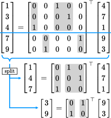
Figure 7: A split process of $\mathbf{P}$

As presented in (14) and Proposition 1, the permutation matrix for the error-free DSF is a discretized doubly-stochastic matrix, which can be denoted as $\mathbf{P}_{\mathrm{hard}}$, in a forward pass, and is differentiable in a backward pass. Here, we show an interesting proposition of $\mathbf{P}_{\mathrm{hard}}$:

Proposition 4.

Let $\mathbf{s}\in\mathbb{R}^{n}$ and $\mathbf{P}_{\mathrm{hard}}\in\mathbb{R}^{n\times n}$ be an unordered sequence and its corresponding permutation matrix to transform to $\mathbf{s}_{\mathrm{o}}$, respectively. We are able to split $\mathbf{s}$ to two subsequences $\mathbf{s}_{1}\in\mathbb{R}^{n_{1}}$ and $\mathbf{s}_{2}\in\mathbb{R}^{n_{2}}$ where $\mathbf{s}_{1}=[\mathbf{s}]_{1:n_{1}}$ and $\mathbf{s}_{2}=[\mathbf{s}]_{n_{1}+1:n_{1}+n_{2}}$. Then, $\mathbf{P}_{\mathrm{hard}}$ is also split to $\mathbf{P}_{1}\in\mathbb{R}^{n_{1}\times n_{1}}$ and $\mathbf{P}_{2}\in\mathbb{R}^{n_{2}\times n_{2}}$, so that $\mathbf{P}_{1}$ and $\mathbf{P}_{2}$ are (discretized) doubly-stochastic.

Proof.

Since a split does not change the relative order of elements in the same split and entries in the permutation matrix is zero or one, a permutation matrix can be split as shown in Figure 7. Moreover, multiple splits are straightforwardly available. ∎

In contrast to $\mathbf{P}_{\mathrm{hard}}$, it is impossible to split $\mathbf{P}_{\mathrm{soft}}$ to sub-block matrices since such sub-block matrices cannot satisfy the property of doubly-stochastic matrix, which is discussed in Proposition 1. Importantly, Proposition 4 does not show a possibility of the recoverable decomposition of the permutation matrix, which implies that we cannot guarantee the recovery of decomposed matrices to the original matrix. Regardless of the existence of recoverable decomposition, we intend to reduce the number of possible permutations with sub-block matrices, rather than holding the large number of possible permutations with the original permutation matrix. Therefore, by Proposition 4, relative relationships between instances with a smaller number of possible permutations are more distinctively learnable than the relationships with a larger number of possible permutations, preventing a sparse correct permutation among a large number of possible permutations.

Appendix H Details of Architectures

We describe the details of the neural architectures used in our paper, as shown in Tables 5, 6, 7, 8, 9, 10, 11, 12, 13, and 14. For the experiments of image fragments, we omit some of the architectures with particular fragmentation, since they follow the same architectures presented in Tables 11, 12, 13, and 14. Only differences are the size of inputs, and therefore the respective sizes of the first fully-connected layers are changed.

Table 5: Architecture of the convolutional neural networks for the four-digit MNIST dataset

Layer	Input & Output (Channel) Dimensions	Kernel Size	Details
Convolutional	$1\times 32$	$5\times 5$	strides 1, padding 2
ReLU	–	–	–
Max-pooling	–	–	pooling 2, strides 2
Convolutional	$32\times 64$	$5\times 5$	strides 1, padding 2
ReLU	–	–	–
Max-pooling	–	–	pooling 2, strides 2
Fully-connected	$12544\times 64$	–	–
ReLU	–	–	–
Fully-connected	$64\times 1$	–	–

Table 6: Architecture of the Transformer-Small models for the four-digit MNIST dataset

Layer	Input & Output (Channel) Dimensions	Kernel Size	Details
Convolutional	$1\times 32$	$5\times 5$	strides 1, padding 2
ReLU	–	–	–
Max-pooling	–	–	pooling 2, strides 2
Convolutional	$32\times 64$	$5\times 5$	strides 1, padding 2
ReLU	–	–	–
Max-pooling	–	–	pooling 2, strides 2
Fully-connected	$12544\times 16$	–	–
Transformer Encoder	$16\times 16$		#layers 6, #heads 8
ReLU	–	–	–
Fully-connected	$16\times 1$	–	–

Table 7: Architecture of the Transformer-Large models for the four-digit MNIST dataset

Layer	Input & Output (Channel) Dimensions	Kernel Size	Details
Convolutional	$1\times 32$	$5\times 5$	strides 1, padding 2
ReLU	–	–	–
Max-pooling	–	–	pooling 2, strides 2
Convolutional	$32\times 64$	$5\times 5$	strides 1, padding 2
ReLU	–	–	–
Max-pooling	–	–	pooling 2, strides 2
Fully-connected	$12544\times 64$	–	–
Transformer Encoder	$64\times 64$		#layers 8, #heads 8
ReLU	–	–	–
Fully-connected	$64\times 1$	–	–

Table 8: Architecture of the convolutional neural networks for the SVHN dataset

Layer	Input & Output (Channel) Dimensions	Kernel Size	Details
Convolutional	$3\times 32$	$5\times 5$	strides 1, padding 2
ReLU	–	–	–
Max-pooling	–	–	pooling 2, strides 2
Convolutional	$32\times 64$	$5\times 5$	strides 1, padding 2
ReLU	–	–	–
Max-pooling	–	–	pooling 2, strides 2
Convolutional	$64\times 128$	$5\times 5$	strides 1, padding 2
ReLU	–	–	–
Max-pooling	–	–	pooling 2, strides 2
Convolutional	$128\times 256$	$5\times 5$	strides 1, padding 2
ReLU	–	–	–
Max-pooling	–	–	pooling 2, strides 2
Fully-connected	$2304\times 64$	–	–
ReLU	–	–	–
Fully-connected	$64\times 1$	–	–

Table 9: Architecture of the Transformer-Small models for the SVHN dataset

Layer	Input & Output (Channel) Dimensions	Kernel Size	Details
Convolutional	$3\times 32$	$5\times 5$	strides 1, padding 2
ReLU	–	–	–
Max-pooling	–	–	pooling 2, strides 2
Convolutional	$32\times 64$	$5\times 5$	strides 1, padding 2
ReLU	–	–	–
Max-pooling	–	–	pooling 2, strides 2
Convolutional	$64\times 64$	$5\times 5$	strides 1, padding 2
ReLU	–	–	–
Max-pooling	–	–	pooling 2, strides 2
Convolutional	$64\times 128$	$5\times 5$	strides 1, padding 2
ReLU	–	–	–
Max-pooling	–	–	pooling 2, strides 2
Fully-connected	$1152\times 32$	–	–
Transformer Encoder	$32\times 32$		#layers 6, #heads 8
ReLU	–	–	–
Fully-connected	$32\times 1$	–	–

Table 10: Architecture of the Transformer-Large models for the SVHN dataset

Layer	Input & Output (Channel) Dimensions	Kernel Size	Details
Convolutional	$3\times 32$	$5\times 5$	strides 1, padding 2
ReLU	–	–	–
Max-pooling	–	–	pooling 2, strides 2
Convolutional	$32\times 64$	$5\times 5$	strides 1, padding 2
ReLU	–	–	–
Max-pooling	–	–	pooling 2, strides 2
Convolutional	$64\times 128$	$5\times 5$	strides 1, padding 2
ReLU	–	–	–
Max-pooling	–	–	pooling 2, strides 2
Convolutional	$128\times 256$	$5\times 5$	strides 1, padding 2
ReLU	–	–	–
Max-pooling	–	–	pooling 2, strides 2
Fully-connected	$2304\times 64$	–	–
Transformer Encoder	$64\times 64$		#layers 8, #heads 8
ReLU	–	–	–
Fully-connected	$64\times 1$	–	–

Table 11: Architecture of the convolutional neural networks for the MNIST dataset of 4 image fragments of size $14\times 14$

Layer	Input & Output (Channel) Dimensions	Kernel Size	Details
Convolutional	$1\times 32$	$3\times 3$	strides 2, padding 1
ReLU	–	–	–
Convolutional	$32\times 64$	$3\times 3$	strides 2, padding 1
ReLU	–	–	–
Fully-connected	$1024\times 64$	–	–
ReLU	–	–	–
Fully-connected	$64\times 1$	–	–

Table 12: Architecture of the Transformer models for the MNIST dataset of 4 image fragments of size $14\times 14$

Layer	Input & Output (Channel) Dimensions	Kernel Size	Details
Convolutional	$1\times 32$	$3\times 3$	strides 2, padding 1
ReLU	–	–	–
Convolutional	$32\times 32$	$3\times 3$	strides 2, padding 1
ReLU	–	–	–
Fully-connected	$512\times 16$	–	–
Transformer Encoder	$16\times 16$		#layers 1, #heads 8
ReLU	–	–	–
Fully-connected	$16\times 1$	–	–

Table 13: Architecture of the convolutional neural networks for the CIFAR-10 dataset of 4 image fragments of size $16\times 16$

Layer	Input & Output (Channel) Dimensions	Kernel Size	Details
Convolutional	$3\times 32$	$3\times 3$	strides 2, padding 1
ReLU	–	–	–
Convolutional	$32\times 64$	$3\times 3$	strides 2, padding 1
ReLU	–	–	–
Fully-connected	$1024\times 64$	–	–
ReLU	–	–	–
Fully-connected	$64\times 1$	–	–

Table 14: Architecture of the Transformer models for the CIFAR-10 dataset of 4 image fragments of size $16\times 16$

Layer	Input & Output (Channel) Dimensions	Kernel Size	Details
Convolutional	$3\times 32$	$3\times 3$	strides 2, padding 1
ReLU	–	–	–
Convolutional	$32\times 32$	$3\times 3$	strides 2, padding 1
ReLU	–	–	–
Fully-connected	$512\times 16$	–	–
Transformer Encoder	$16\times 16$		#layers 1, #heads 8
ReLU	–	–	–
Fully-connected	$16\times 1$	–	–

Appendix I Details of Experiments

As described in the main article, we use three public datasets: MNIST (LeCun et al., 1998), SVHN (Netzer et al., 2011), and CIFAR-10 (Krizhevsky & Hinton, 2009). Unless otherwise specified, the learning rate $10^{-3.5}$ is used for the CNN architectures and the learning rate $10^{-4}$ is used for the Transformer-based architectures; see the scripts for the exact learning rates we use in the experiments. Learning rate decay is applied to multiply $0.5$ in every 50,000 steps for the experiments on sorting multi-digit images and every 20,000 steps for the experiments on sorting image fragments. Moreover, we balance two objectives for $\mathbf{P}_{\mathrm{hard}}$ and $\mathbf{P}_{\mathrm{soft}}$ by multiplying $1$, $0.1$, $0.01$, or $0.001$; see the scripts included in our implementation for the respective values for all the experiments. For random seeds, we pick five random seeds for all the experiments: $42$, $84$, $126$, $168$, and $210$; these values are picked without any trials. Other missing details can be found in our implementation, which is included alongside our manuscript. Furthermore, we use several commercial NVIDIA GPUs, i.e., GeForce GTX Titan Xp, GeForce RTX 2080, and GeForce RTX 3090, for the experiments.

Appendix J Study on Balancing Hyperparameter

We conduct a study on a balancing hyperparameter in the experiments on sorting the four-digit MNIST dataset, as shown in Table 15. For these experiments, we use steepness 6, 20, 29, 32, 25, and 124 for sequence lengths 3, 5, 7, 9, 15, and 32, respectively. Also, we use a learning rate $10^{-3}$ and five random seeds 42, 84, 126, 168, and 210.

Table 15: Study on a balancing hyperparameter $\lambda$ in the experiments of sorting the four-digit MNIST dataset

$\boldsymbol{\lambda}$	Sequence Length
	3	5	7	9	15	32
1.000	94.9 (96.5)	86.1 (93.8)	73.7 (90.6)	60.8 (87.9)	10.8 (67.8)	0.0 (31.8)
0.100	94.8 (96.4)	86.4 (93.8)	75.3 (91.2)	65.6 (89.6)	33.7 (83.0)	1.2 (63.0)
0.010	94.9 (96.5)	87.2 (94.2)	76.3 (91.6)	65.6 (89.5)	32.9 (82.8)	0.8 (62.6)
0.001	95.2 (96.7)	86.6 (94.0)	75.3 (91.2)	64.6 (89.1)	34.4 (83.2)	1.4 (66.4)
0.000	94.8 (96.4)	86.6 (93.9)	76.4 (91.7)	64.0 (89.0)	33.0 (82.6)	1.3 (66.0)

Appendix K Study on Steepness and Learning Rate

We present studies on steepness and learning rate for the experiments on sorting the multi-digit MNIST dataset, as shown in Tables 16, 17, 18, 19, 20, and 21. For these experiments, a random seed 42 is only used due to numerous experimental settings. Also, we use balancing hyperparameters $\lambda$ as 1.0, 1.0, 0.1, 0.1, 0.1, and 0.1 for sequence lengths 3, 5, 7, 9, 15, and 32, respectively. Since there are many configurations of steepness, learning rate, and a balancing hyperparameter, we cannot include all the configurations here. The final configurations we use in the experiments are described in our implementation.

Table 16: Study on steepness and learning rate for a sequence length 3. lr stands for learning rate.

${\boldsymbol{\log}}_{\textbf{10}}$ lr	Steepness
	2	4	6	8	10	12	14
-4.0	89.2 (92.6)	91.5 (94.2)	92.1 (94.6)	92.3 (94.7)	92.7 (95.0)	92.1 (94.6)	92.7 (95.0)
-3.5	93.6 (95.5)	93.4 (95.5)	94.5 (96.2)	93.9 (95.9)	94.4 (96.1)	94.5 (96.2)	94.6 (96.3)
-3.0	95.3 (96.8)	95.1 (96.6)	95.0 (96.5)	94.4 (96.2)	94.3 (96.1)	94.7 (96.4)	94.8 (96.5)
-2.5	94.5 (96.2)	94.3 (96.1)	93.7 (95.6)	93.8 (95.7)	93.7 (95.7)	93.7 (95.6)	94.1 (95.9)

Table 17: Study on steepness and learning rate for a sequence length 5. lr stands for learning rate.

${\boldsymbol{\log}}_{\textbf{10}}$ lr	Steepness
	14	16	18	20	22	24	26
-4.0	78.3 (90.2)	76.3 (89.3)	79.5 (90.9)	78.7 (90.4)	78.4 (90.4)	77.3 (89.8)	79.0 (90.6)
-3.5	85.1 (93.3)	83.6 (92.7)	84.8 (93.1)	85.5 (93.5)	83.4 (92.5)	85.6 (93.6)	84.1 (92.8)
-3.0	86.9 (94.1)	85.2 (93.3)	86.2 (93.8)	85.7 (93.6)	85.4 (93.5)	85.0 (93.2)	85.0 (93.3)
-2.5	83.1 (92.3)	83.2 (92.4)	83.1 (92.4)	81.7 (91.8)	83.3 (92.5)	82.4 (92.1)	82.5 (92.1)

Table 18: Study on steepness and learning rate for a sequence length 7. lr stands for learning rate.

${\boldsymbol{\log}}_{\textbf{10}}$ lr	Steepness
	23	25	27	29	31	33	35
-4.0	53.5 (82.9)	57.3 (84.6)	61.0 (86.0)	58.3 (85.1)	66.1 (88.0)	57.3 (84.6)	61.6 (86.4)
-3.5	71.6 (90.0)	73.5 (90.8)	68.1 (88.6)	72.9 (90.5)	72.2 (90.2)	71.4 (89.9)	74.2 (91.0)
-3.0	74.4 (90.9)	72.8 (90.4)	74.2 (90.8)	69.2 (89.0)	69.9 (89.3)	73.0 (90.4)	73.0 (90.5)
-2.5	68.0 (88.6)	67.2 (88.1)	68.1 (88.6)	64.5 (86.9)	66.8 (88.0)	70.4 (89.3)	66.2 (87.9)

Table 19: Study on steepness and learning rate for a sequence length 9. lr stands for learning rate.

${\boldsymbol{\log}}_{\textbf{10}}$ lr	Steepness
	26	28	30	32	34	36	38
-4.0	34.0 (77.7)	37.8 (79.7)	37.3 (79.4)	45.9 (83.0)	46.4 (83.1)	36.2 (78.9)	45.3 (82.5)
-3.5	51.8 (84.8)	59.7 (87.5)	58.3 (87.5)	61.0 (88.2)	60.2 (88.1)	54.6 (85.8)	56.3 (86.6)
-3.0	62.5 (88.8)	60.5 (88.0)	61.8 (88.4)	63.2 (88.9)	61.5 (88.2)	62.2 (88.6)	65.0 (89.5)
-2.5	57.4 (86.8)	58.7 (87.2)	56.5 (86.4)	55.3 (86.1)	52.8 (85.0)	46.9 (82.1)	52.1 (84.6)

Table 20: Study on steepness and learning rate for a sequence length 15. lr stands for learning rate.

${\boldsymbol{\log}}_{\textbf{10}}$ lr	Steepness
	19	21	23	25	27	29	31
-4.0	3.6 (62.7)	7.2 (67.6)	4.9 (64.8)	2.6 (60.9)	2.9 (61.5)	2.5 (60.2)	6.8 (68.3)
-3.5	10.3 (71.5)	11.9 (73.0)	7.6 (68.6)	22.3 (78.7)	7.1 (68.7)	8.2 (69.6)	10.6 (71.8)
-3.0	24.2 (79.8)	24.1 (80.1)	29.7 (81.9)	32.1 (82.7)	23.9 (79.9)	31.6 (82.1)	31.0 (82.0)
-2.5	30.5 (81.4)	28.2 (80.0)	18.9 (76.8)	29.8 (80.9)	19.8 (77.8)	15.4 (75.4)	24.6 (79.6)

Table 21: Study on steepness and learning rate for a sequence length 32. lr stands for learning rate.

${\boldsymbol{\log}}_{\textbf{10}}$ lr	Steepness
	118	120	122	124	126	128	130
-4.0	0.0 (46.4)	0.0 (45.8)	0.0 (46.4)	0.0 (43.1)	0.0 (42.9)	0.0 (49.4)	0.0 (48.9)
-3.5	0.2 (60.5)	0.3 (61.8)	0.7 (64.8)	0.3 (62.7)	0.0 (56.0)	0.3 (62.7)	0.2 (59.8)
-3.0	0.6 (63.1)	0.5 (63.6)	0.4 (59.8)	0.8 (65.8)	0.2 (58.1)	0.1 (56.0)	0.1 (57.1)
-2.5	0.5 (62.8)	0.5 (62.3)	0.5 (62.5)	0.1 (58.3)	0.3 (61.2)	0.1 (59.5)	0.2 (58.1)

Appendix L Limitations

Because our methods are based on a sorting network, our ideas are limited to sorting algorithms. It implies that it is not easy to devise a neural network-based approach to solving general problems in computer science, e.g., combinatorial optimization, with our ideas.

Appendix M Broader Impacts

Since our work proposes a method to sort high-dimensional instances in a sequence using a differentiable swap function, a direct negative societal impact does not exist. However, there can be a potential issue of sorting controversial high-dimensional data that is considered not to be sorted, e.g., beauty and intelligence.

References

- Ajtai et al. (1983) M. Ajtai, J. Komlós, and E. Szemerédi. An O(n log n) sorting network. In Proceedings of the Annual ACM Symposium on Theory of Computing (STOC), pp. 1–9, Boston, Massachusetts, USA, 1983.
- Ba et al. (2016) J. L. Ba, J. R. Kiros, and G. E. Hinton. Layer normalization. arXiv preprint arXiv:1607.06450, 2016.
- Bengio et al. (2013) Y. Bengio, N. Léonard, and A. Courville. Estimating or propagating gradients through stochastic neurons for conditional computation. arXiv preprint arXiv:1308.3432, 2013.
- Blondel et al. (2020) M. Blondel, O. Teboul, Q. Berthet, and J. Djolonga. Fast differentiable sorting and ranking. In Proceedings of the International Conference on Machine Learning (ICML), pp. 950–959, Virtual, 2020.
- Brown et al. (2020) T. B. Brown, B. Mann, N. Ryder, M. Subbiah, J. Kaplan, P. Dhariwal, A. Neelakantan, P. Shyam, G. Sastry, A. Askell, S. Agarwal, A. Herbert-Voss, G. Krueger, T. Henighan, R. Child, A. Ramesh, D. M. Ziegler, J. Wu, C. Winter, C. Hesse, M. Chen, E. Sigler, M. Litwin, S. Gray, B. Chess, J. Clark, C. Berner, S. McCandlish, A. Radford, I. Sutskever, and D. Amodei. Language models are few-shot learners. In Advances in Neural Information Processing Systems (NeurIPS), volume 33, pp. 1877–1901, Virtual, 2020.
- Cormen et al. (2022) T. H. Cormen, C. E. Leiserson, R. L. Rivest, and C. Stein. Introduction to algorithms. MIT Press, 4 edition, 2022.
- Cuturi (2013) M. Cuturi. Sinkhorn distances: lightspeed computation of optimal transport. In Advances in Neural Information Processing Systems (NeurIPS), volume 26, pp. 2292–2300, Lake Tahoe, Nevada, USA, 2013.
- Cuturi et al. (2019) M. Cuturi, O. Teboul, and J.-P. Vert. Differentiable ranking and sorting using optimal transport. In Advances in Neural Information Processing Systems (NeurIPS), volume 32, Vancouver, British Columbia, Canada, 2019.
- Devlin et al. (2018) J. Devlin, M.-W. Chang, K. Lee, and K. Toutanova. BERT: Pre-training of deep bidirectional transformers for language understanding. arXiv preprint arXiv:1810.04805, 2018.
- Dosovitskiy et al. (2021) A. Dosovitskiy, L. Beyer, A. Kolesnikov, D. Weissenborn, X. Zhai, T. Unterthiner, M. Dehghani, M. Minderer, G. Heigold, S. Gelly, J. Uszkoreit, and N. Houlsby. An image is worth 16x16 words: Transformers for image recognition at scale. In Proceedings of the International Conference on Learning Representations (ICLR), Virtual, 2021.
- Grover et al. (2019) A. Grover, E. Wang, A. Zweig, and S. Ermon. Stochastic optimization of sorting networks via continuous relaxations. In Proceedings of the International Conference on Learning Representations (ICLR), New Orleans, Louisiana, USA, 2019.
- He et al. (2016) K. He, X. Zhang, S. Ren, and J. Sun. Deep residual learning for image recognition. In Proceedings of the IEEE International Conference on Computer Vision and Pattern Recognition (CVPR), pp. 770–778, Las Vegas, Nevada, USA, 2016.
- Hochreiter & Schmidhuber (1997) S. Hochreiter and J. Schmidhuber. Long short-term memory. Neural Computation, 9(8):1735–1780, 1997.
- Knuth (1998) D. E. Knuth. The art of computer programming, volume 3. Addison-Wesley Professional, 2 edition, 1998.
- Krizhevsky & Hinton (2009) A. Krizhevsky and G. E. Hinton. Learning multiple layers of features from tiny images. Technical report, Computer Science Department, University of Toronto, 2009.
- LeCun et al. (1998) Y. LeCun, C. Cortes, and C. J. C. Burges. The MNIST database of handwritten digits. http://yann.lecun.com/exdb/mnist/, 1998.
- Lee et al. (2019) J. Lee, Y. Lee, J. Kim, A. R. Kosiorek, S. Choi, and Y. W. Teh. Set Transformer: A framework for attention-based permutation-invariant neural networks. In Proceedings of the International Conference on Machine Learning (ICML), pp. 3744–3753, Long Beach, California, USA, 2019.
- Liu et al. (2021) Z. Liu, Y. Lin, Y. Cao, H. Hu, Y. Wei, Z. Zhang, S. Lin, and B. Guo. Swin Transformer: Hierarchical vision transformer using shifted windows. In Proceedings of the International Conference on Computer Vision (ICCV), pp. 10012–10022, Virtual, 2021.
- Loshchilov & Hutter (2018) I. Loshchilov and F. Hutter. Decoupled weight decay regularization. In Proceedings of the International Conference on Learning Representations (ICLR), Vancouver, British Columbia, Canada, 2018.
- Mena et al. (2018) G. E. Mena, D. Belanger, S. Linderman, and J. Snoek. Learning latent permutations with Gumbel-Sinkhorn networks. In Proceedings of the International Conference on Learning Representations (ICLR), Vancouver, British Columbia, Canada, 2018.
- Nash et al. (2020) C. Nash, Y. Ganin, S. M. A. Eslami, and P. W. Battaglia. PolyGen: An autoregressive generative model of 3D meshes. In Proceedings of the International Conference on Machine Learning (ICML), pp. 7220–7229, Virtual, 2020.
- Netzer et al. (2011) Y. Netzer, T. Wang, A. Coates, A. Bissacco, B. Wu, and A. Y. Ng. Reading digits in natural images with unsupervised feature learning. In Neural Information Processing Systems Workshop on Deep Learning and Unsupervised Feature Learning, Granada, Spain, 2011.
- Petersen et al. (2021) F. Petersen, C. Borgelt, H. Kuehne, and O. Deussen. Differentiable sorting networks for scalable sorting and ranking supervision. In Proceedings of the International Conference on Machine Learning (ICML), pp. 8546–8555, Virtual, 2021.
- Petersen et al. (2022) F. Petersen, C. Borgelt, H. Kuehne, and O. Deussen. Monotonic differentiable sorting networks. In Proceedings of the International Conference on Learning Representations (ICLR), Virtual, 2022.
- Sutskever et al. (2014) I. Sutskever, O. Vinyals, and Q. V. Le. Sequence to sequence learning with neural networks. In Advances in Neural Information Processing Systems (NeurIPS), volume 27, Montreal, Quebec, Canada, 2014.
- Vaswani et al. (2017) A. Vaswani, N. Shazeer, N. Parmar, J. Uszkoreit, L. Jones, A. N. Gomez, Ł. Kaiser, and I. Polosukhin. Attention is all you need. In Advances in Neural Information Processing Systems (NeurIPS), volume 30, pp. 5998–6008, Long Beach, California, USA, 2017.
- Vinyals et al. (2016) O. Vinyals, S. Bengio, and M. Kudlur. Order matters: Sequence to sequence for sets. In Proceedings of the International Conference on Learning Representations (ICLR), San Juan, Puerto Rico, 2016.
- Zaheer et al. (2017) M. Zaheer, S. Kottur, S. Ravanbakhsh, B. Poczos, R. R. Salakhutdinov, and A. J. Smola. Deep sets. In Advances in Neural Information Processing Systems (NeurIPS), volume 30, pp. 3391–3401, Long Beach, California, USA, 2017.
- Zhao et al. (2021) H. Zhao, L. Jiang, J. Jia, P. Torr, and V. Koltun. Point transformer. In Proceedings of the International Conference on Computer Vision (ICCV), pp. 16259–16268, Virtual, 2021.