Exponential Quantum Communication Advantage in Distributed Learning

Abstract

Training and inference with large machine learning models that far exceed the memory capacity of individual devices necessitates the design of distributed architectures, forcing one to contend with communication constraints. We present a framework for distributed computation over a quantum network in which data is encoded into specialized quantum states. We prove that for certain models within this framework, inference and training using gradient descent can be performed with exponentially less communication compared to their classical analogs, and with relatively modest time and space complexity overheads relative to standard gradient-based methods. To our knowledge, this is the first example of exponential quantum advantage for a generic class of machine learning problems with dense classical data that holds regardless of the data encoding cost. Moreover, we show that models in this class can encode highly nonlinear features of their inputs, and their expressivity increases exponentially with model depth. We also find that, interestingly, the communication advantage nearly vanishes for simpler linear classifiers. These results can be combined with natural privacy advantages in the communicated quantum states that limit the amount of information that can be extracted from them about the data and model parameters. Taken as a whole, these findings form a promising foundation for distributed machine learning over quantum networks.

1 Introduction

As the scale of the datasets and parameterized models used to perform computation over data continues to grow [54, 44], distributing workloads across multiple devices becomes essential for enabling progress. The choice of architecture for large-scale training and inference must not only make the best use of computational and memory resources, but also contend with the fact that communication may become a bottleneck [86]. When using modern optical interconnects, classical computers exchange bits represented by light. This however does not fully utilize the potential of the physical substrate; given suitable computational capabilities and algorithms, the quantum nature of light can be harnessed as a powerful communication resource. Here we show that for a broad class of parameterized models, if quantum bits (qubits) are communicated instead of classical bits, an exponential reduction in the communication required to perform inference and gradient-based training can be achieved. This protocol additionally guarantees improved privacy of both the user data and model parameters through natural features of quantum mechanics, without the need for additional cryptographic or privacy protocols. To our knowledge, this is the first example of generic, exponential quantum advantage on problems that occur naturally in the training and deployment of large machine learning models. These types of communication advantages help scope the future roles and interplay between quantum and classical communication for distributed machine learning.

Quantum computers promise dramatic speedups across a number of computational tasks, with perhaps the most prominent example being the ability revolutionize our understanding of nature by enabling the simulation of quantum systems, owing to the natural similarity between quantum computers and the world [35, 64]. However, much of the data that one would like to compute with in practice seems to come from an emergent classical world rather than directly exhibiting quantum properties. While there are some well-known examples of exponential quantum speedups for classical problems, most famously factoring [94] and related hidden subgroup problems [29], these tend to be isolated and at times difficult to relate to practical applications. In addition, even though significant speedups are known for certain ubiquitous problems in machine learning such as matrix inversion [42] and principal component analysis [65], the advantage is often lost when including the cost of loading classical data into the quantum computer or of reading out the result into classical memory [2]. In applications where an efficient data access model avoids the above pitfalls, the complexity of quantum algorithms tends to depend on condition numbers of matrices which scale with system size in a way that reduces or even eliminates any quantum advantage [73]. It is worth noting that much of the discussion about the impact of quantum technology on machine learning has focused on computational advantage. However quantum resources are not only useful in reducing computational complexity — they can also provide an advantage in communication complexity, enabling exponential reductions in communication for some problems [90, 15]. Inspired by these results, we study a setting where quantum advantage in communication is possible across a wide class of machine learning models. This advantage holds without requiring any sparsity assumptions or elaborate data access models such as QRAM [37].

We focus on compositional distributed learning, known as pipelining [48, 16]. While there are a number of strategies for distributing machine learning workloads that are influenced by the requirements of different applications and hardware constraints [100, 53], splitting up a computational graph in a compositional fashion (Figure 1) is a common approach. We describe distributed, parameterized quantum circuits that can be used to perform inference over data when distributed in this way, and can be trained using gradient methods. The ideas we present can also be used to optimize models that use certain forms of data parallelism (Appendix C). In principle, such circuits could be implemented on quantum computers that are able to communicate quantum states.

For the general class of distributed, parameterized quantum circuits that we study, we show the following:

• Even for simple circuits in this class, there is an exponential quantum advantage in communication for the problem of estimating the loss and the gradients of the loss with respect to the parameters (Section 3). This additionally implies a privacy advantage from Holevo’s bound (Section 6). We also show that this is advantage is not a trivial consequence of the data encoding used, since it does not hold for certain problems like linear classification (Appendix E).

• For a subclass of these circuits, there is an exponential advantage in communication for the entire training process, and not just for a single round of gradient estimation. This subclass includes circuits for fine-tuning using pre-trained features. The proof is based on convergence rates for stochastic gradient descent under convexity assumptions (Section 4).

• The ability to interleave multiple unitaries encoding nonlinear features of data enables expressivity to grow exponentially with depth, and universal function approximation in some settings. This implies that these models are highly expressive in contrast to popular belief about linear restrictions in quantum neural networks (Section 5).

2 Preliminaries

2.1 Large-scale learning problems and distributed computation

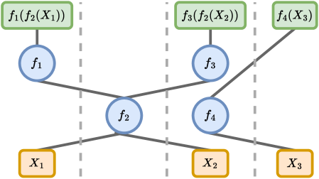
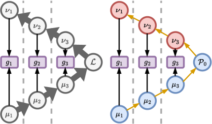
Figure 1: Left: Distributed, compositional computation. Dashed lines separate devices with computational and storage resources. The circular nodes represent parameterized functions that are allocated distinct hardware resources and are spatially separated, while the square nodes represent data (yellow) and outputs corresponding to different tasks (green). The vertical axis represents time. This framework of hardware allocation enables flexible modification of the model structure in a task-dependent fashion. Right: Computation of gradient estimators $g_{\ell}$ at different layers of a model distributed across multiple devices by pipelining. Computing forward features $\mu_{\ell}$ and backwards features $\nu_{\ell}$ (also known as computing a forward or backward pass) requires a large amount of classical communication (grey) but an exponentially smaller amount of quantum communication (yellow). $\mathcal{L}$ is the classical loss function, and $\mathcal{P}_{0}$ an operator whose expectation value with respect to a quantum model gives the analogous loss function in the quantum case.

Pipelining is a commonly used method of distributing a machine learning workload, in which different layers of a deep model are allocated distinct hardware resources [48, 78]. Training and inference then require communication of features between nodes. Pipelining enables flexible changes to the model architecture in a task-dependent manner, since subsets of a large model can be combined in an adaptive fashion to solve many downstream tasks. Additionally, pipelining allows sparse activation of a subset of a model required to solve a task, and facilitates better use of heterogeneous compute resources since it does not require storing identical copies of a large model. The potential for large models to be easily fine-tuned to solve multiple tasks is well-known [23, 19], and pipelined architectures which facilitate this are the norm in the latest generation of large language models [88, 16]. Data parallelism, in contrast, involves storing multiple copies of the model on different nodes, training each on a subsets of the data and exchanging information to synchronize parameter updates. In practice, different parallelization strategies are combined in order to exploit trade-offs between latency and throughput in a task-dependent fashion [100, 53, 86]. Distributed quantum models were considered recently in [83], but the potential for quantum advantage in communication in these settings was not discussed.

2.2 Communication complexity

Communication complexity [101, 57, 87] is the study of distributed computational problems using a cost model that focuses on the communication required between players rather than the time or computational complexity. It is naturally related to the study of the space complexity of streaming algorithms [92]. The key object of study in this area is the tree induced by a communication protocol whose nodes enumerate all possible communication histories and whose leaves correspond to the outputs of the protocol. The product structure induced on the leaves of this tree as a function of the inputs allows one to bound the depth of the tree from below, which gives an unconditional lower bound on the communication complexity. The power of replacing classical bits of communication with qubits has been the subject of extensive study [28, 21, 25]. For certain problems such as Hidden Matching [15] and a variant of classification with deep linear models [90] an exponential quantum communication advantage holds, while for other canonical problems such as Disjointness only a polynomial advantage is possible [91]. Exponential advantage was also recently shown for the problem of sampling from a distribution defined by the solution to a linear regression problem [74].

At a glance, the development of networked quantum computers may seem much more challenging than the already herculean task of building a fault tolerant quantum computer. However, for some quantum network architectures, the existence of a long-lasting fault tolerant quantum memory as a quantum repeater, may be the enabling component that lifts low rate shared entanglement to a fully functional quantum network [77], and hence the timelines for small fault tolerant quantum computers and quantum networks may be more coincident than it might seem at first. As such, it is well motivated to consider potential communication advantages alongside computational advantages when talking about the applications of fault tolerant quantum computers. In Appendix G we briefly survey approaches to implementing quantum communication in practice, and the associated challenges.

In addition, while we largely restrict ourselves here to discussions of communication advantages, and most other studies focus on purely computational advantages, there may be interesting advantages at their intersection. For example, it is known that no quantum state built from a simple (or polynomial complexity) circuit can confer an exponential communication advantage, however states made from simple circuits can be made computationally difficult to distinguish [51]. Hence the use of quantum pre-computation [49] and communication may confer advantages even when traditional computational and communication cost models do not admit such advantages due to their restriction in scope.

3 Distributed learning with quantum resources

In this work we focus on parameterized models that are representative of the most common models used and studied today in quantum machine learning, sometimes referred to as quantum neural networks [70, 34, 26, 93]. We will use the standard Dirac notation of quantum mechanics throughout. A summary of relevant notation and the fundamentals of quantum mechanics is provided in Appendix A. We define a class models with parameters $\Theta$, taking an input $x$ which is a tensor of size $N$. The models take the following general form:

Definition 3.1.

$\{A_{\ell}(\theta^{A}_{\ell},x)\},\{B_{\ell}(\theta^{B}_{\ell},x)\}$ for $\ell\in\{1,\dots,L\}$ are each a set of unitary matrices of size $N^{\prime}\times N^{\prime}$ for some $N^{\prime}$ such that $\log N^{\prime}=O(\log N)$ . The $\theta_{\ell}^{A},\theta_{\ell}^{B}$ are vectors of $P$ parameters each. For every $\ell,i$, we assume that $\frac{\partial A_{\ell}}{\partial\theta_{\ell i}^{A}}$ is anti-hermitian up to a real scaling factor and has at most two eigenvalues, and similarly for $B_{\ell}$.

The model we consider is defined by

$$\left|\varphi(\Theta,x)\right\rangle\equiv\left(\underset{\ell=L}{\overset{1}{\prod}}A_{\ell}(\theta^{A}_{\ell},x)B_{\ell}(\theta^{B}_{\ell},x)\right)\left|\psi(x)\right\rangle,$$ (3.1)

where $\psi(x)$ is a fixed state of $\log N^{\prime}$ qubits.

The loss function is given by

$$\mathcal{L}(\Theta,x)\equiv\left\langle\varphi(\Theta,x)\right|\mathcal{P}_{0}\left|\varphi(\Theta,x)\right\rangle,$$ (3.2)

where $\mathcal{P}_{0}$ is a Pauli matrix that acts on the first qubit.

In standard linear algebra notation, the output of the model is a unit norm $N^{\prime}$-dimensional complex vector $\varphi_{L}$, defined recursively by

$$\varphi_{0}=\psi(x),\quad\varphi_{\ell}=A_{\ell}(\theta_{\ell}^{A},x)B_{\ell}(\theta_{\ell}^{B},x)\varphi_{\ell-1},$$ (3.3)

where the entries of $\varphi_{L}$ are represented by the amplitudes of a quantum state. The loss takes the form $\mathcal{L}(\Theta,x)=\left(\varphi_{L}^{\ast}\right)^{T}\mathcal{P}_{0}\varphi_{L}$ where ^∗ indicates the entrywise complex conjugate, and this definition includes the standard $L^{2}$ loss as a special case.

Subsequently we omit the dependence on $x$ and $\Theta$ (or subsets of it) to lighten notation, and consider special cases where only subsets of the unitaries depend on $x$, or where the unitaries take a particular form and may not be parameterized. Denote by $\nabla_{A(B)}\mathcal{L}$ the entries of the gradient vector that correspond to the parameters of $\{A_{\ell}\}(\{B_{\ell}\})$.

While seemingly stringent, the condition on the derivatives is in fact satisfied by many of the most common quantum neural network architectures [26, 32, 93]. This condition is satisfied for example if

$$A_{\ell}=\underset{j=1}{\overset{P}{\prod}}e^{i\alpha^{A}_{\ell j}\theta_{\ell j}^{A}\mathcal{P}_{\ell j}^{A}}$$ (3.4)

and the $\mathcal{P}_{\ell j}^{A}$ are both unitary and Hermitian (e.g. Pauli matrices), while $\beta^{A}_{\ell j}$ are scalars. Such models, or parameterized quantum circuits, are naturally amenable to implementation on quantum devices, and for $P=O(N^{2})$ any unitary over $\log N^{\prime}$ qubits can be written in this form. In the special case where $x$ in a unit norm $N$-dimensional vector, a simple choice of $\left|\psi(x)\right\rangle$ is the amplitude encoding of $x$, given by

$$\left|\psi(x)\right\rangle=\left|x\right\rangle=\underset{i=0}{\overset{N-1}{\sum}}x_{i}\left|i\right\rangle.$$ (3.5)

However, despite its exponential compactness in representing the data, a naive implementation of the simplest choice is restricted to representing quadratic features of the data that can offer no substantial quantum advantage in a learning task [47], so the choice of data encoding is critical to the power of a model. The interesting parameter regime for classical data and models is one where $N,P$ are large, while $L$ is relatively modest. For general unitaries $P=O(N^{2})$, which matches the scaling of the number of parameters in fully-connected networks. When the input tensor $x$ is a batch of datapoints, $N$ is equivalent to the product of batch size and input dimension.

The model in Definition 3.1 can be used to define distributed inference and learning problems by dividing the input $x$ and the parameterized unitaries between two players, Alice and Bob. We define their respective inputs as follows:

$$\mathrm{Alice}: \left|\psi(x)\right\rangle,\{A_{\ell}\},$$ (3.6)

$$\mathrm{Bob}: \{B_{\ell}\}.$$

The problems of interest require that Alice and Bob compute certain joint functions of their inputs. As a trivial base case, it is clear that in a communication cost model, all problems can be solved with communication cost at most the size of the inputs times the number of parties, by a protocol in which each party sends its inputs to all others. We will be interested in cases where one can do much better by taking advantage of quantum communication.

Figure 2: Distributed quantum circuit implementing $\mathcal{L}$ for $L=2$. Both $\mathcal{L}$ and its gradients with respect to the parameters of the unitaries can be estimated with total communication that is polylogarithmic in the size of the input data $N$ and the number of trainable parameters per unitary $P$.

Given the inputs eq. 3.6, we will be interested chiefly in the two problems specified below.

Problem 1 (Distributed Inference).

Alice and Bob each compute an estimate of $\left\langle\varphi\right|\mathcal{P}_{0}\left|\varphi\right\rangle$ up to additive error $\varepsilon$.

The straightforward algorithm for this problem, illustrated in fig. 2, requires $L$ rounds of communication. The other problem we consider is the following:

Problem 2 (Distributed Gradient Estimation).

Alice computes an estimate of $\nabla_{A}\left\langle\varphi\right|\mathcal{P}_{0}\left|\varphi\right\rangle$, while Bob computes an estimate of $\nabla_{B}\left\langle\varphi\right|Z_{0}\left|\varphi\right\rangle$, up to additive error $\varepsilon$ in $L^{\infty}$.

3.1 Communication complexity of inference and gradient estimation

We show that inference and gradient estimation are achievable with a logarithmic amount of quantum communication, which will represent an exponential improvement over the classical cost for some cases:

Lemma 1.

1 can be solved by communicating $O(\log N)$ qubits over $O(L/\varepsilon^{2})$ rounds.

Proof: Appendix B.

Lemma 2.

2 can be solved with probability greater than $1-\delta$ by communicating $\tilde{O}(\log N(\log P)^{2}\log(L/\delta)/\varepsilon^{4})$ qubits over $O(L^{2})$ rounds. The time and space complexity of the algorithm is $\sqrt{P}\;L\;\mathrm{poly}(N,\log P,\varepsilon^{-1},\log(1/\delta))$.

Proof: Appendix B.

This upper bound is obtained by simply noting that the problem of gradient estimation at every layer can be reduced to a shadow tomography problem [7]:

Theorem 1 (Shadow Tomography [4] solved with Threshold Search [13]).

For an unknown state $\lvert\psi\rangle$ of $\log N$ qubits, given $K$ known two-outcome measurements $E_{i}$, there is an explicit algorithm that takes $\lvert\psi\rangle^{\otimes k}$ as input, where $k=\tilde{O}(\log^{2}K\log N\log(1/\delta)/\varepsilon^{4})$, and produces estimates of $\left\langle\psi\right|E_{i}\left|\psi\right\rangle$ for all $i$ up to additive error $\varepsilon$ with probability greater than $1-\delta$. $\tilde{O}$ hides subdominant polylog factors.

Using immediate reductions from known problems in communication complexity, we can show that the amount of classical communication required to solve these problem is polynomial in the size of the input, and additionally give a lower bound on the number of rounds of communication required by any quantum or classical algorithm:

Lemma 3.

1. The classical communication complexity of 1 and 2 is $\Omega(\max(\sqrt{N},L))$.

2. Any algorithm (quantum or classical) for 1 or 2 requires either $\Omega(L)$ rounds of communication or $\Omega(N/L^{4})$ qubits (or bits) of communication.

Proof: Appendix B

The implication of the second result in Lemma 3 is that $\Omega(L)$ rounds of communication are necessary in order to obtain an exponential communication advantage for small $L$, since otherwise the number of qubits of communication required can scale linearly with $N$.

Combining Lemma 2 and Lemma 3, in the regime where $L=O(\mathrm{polylog}(N))$, which is relevant for classical machine learning models, we obtain an exponential advantage in communication complexity for both inference and gradient estimation. The required overhead in terms of time and space is only polynomial when compared to the straightforward classical algorithms for these problems.

The distribution of the model as in eq. 3.6 is an example of pipelining. Data parallelism is another common approach to distributed machine learning in which subsets of the data are distributed to identical copies of the model. In Appendix C we show that it can also be implemented using quantum circuits, which can then trained using gradient descent requiring quantum communication that is logarithmic in the number of parameters and input size.

Quantum advantage is possible in these problems because there is a bound on the complexity of the final output, whether it be correlated elements of the gradient up to some finite error or the low-dimensional output of a model. This might lead one to believe that whenever the output takes such a form, encoding the data in the amplitudes of a quantum state will trivially give an exponential advantage in communication complexity. We show however that the situation is slightly more nuanced, by considering the problem of inference with a linear model:

Lemma 4.

For the problem of distributed linear classification, there can be no exponential advantage in using quantum communication in place of classical communication.

The precise statement and proof of this result are presented in Appendix E. This result also highlights that the worst case lower bounds such as Lemma 3 may not hold for circuits with certain low-dimensional or other simplifying structure.

4 Exponential advantages in end-to-end training

So far we have discussed the problems of inference and estimating a single gradient vector. It is natural to also consider when these or other gradient estimators can be used to efficiently solve an optimization problem (i.e. when the entire training processes is considered rather than a single iteration). Applying the gradient estimation algorithm detailed in Lemma 2 iteratively gives a distributed stochastic gradient descent algorithm which we detail in Algorithm 2, yet one may be concerned that a choice of $\varepsilon=O(\log N)$ which is needed to obtain an advantage in communication complexity will preclude efficient convergence. Here we present a simpler algorithm that requires a single quantum measurement per iteration, and can provably solve certain convex problems efficiently, as well as an application of shadow tomography to fine-tuning where convergence can be guaranteed, again with only logarithmic communication cost. In both cases, there is an exponential advantage in communication even when considering the entire training process.

4.1 “Smooth” circuits

Consider the case where $A_{\ell}$ are product of rotations for all $\ell$, namely

$$A_{\ell}=\underset{j=1}{\overset{P}{\prod}}e^{-\frac{1}{2}i\beta^{A}_{\ell j}\theta^{A}_{\ell j}\mathcal{P}_{\ell j}^{A}},$$ (4.1)

where $\mathcal{P}_{\ell j}^{A}$ are Pauli matrices acting on all qubits, and similarly for $B_{\ell}$. These can also be interspersed with other non-trainable unitaries. This constitutes a slight generalization of the setting considered in [43], and the algorithm we present is essentially a distributed distributed version of theirs. Denote by $\beta$ an $2PL$-dimensional vector with elements $\beta^{Q}_{\ell j}$ where $Q\in\{A,B\}$ . The quantity $\left\|\beta\right\|_{1}$ is the total evolution time if we interpret the state $\left|\varphi\right\rangle$ as a sequence of Hamiltonians applied to the initial state $\left|x\right\rangle$.

In Section D.1 we describe an algorithm that converges to the neighborhood of a minimum, or achieves $\mathbb{E}\mathcal{L}(\Theta)-\mathcal{L}(\Theta^{\star})\leq\varepsilon_{0}$, for a convex $\mathcal{L}$ after

$$\frac{2\left\|\Theta^{(0)}-\Theta^{\star}\right\|_{2}^{2}\left\|\beta\right\|_{1}^{2}}{\varepsilon_{0}^{2}}$$ (4.2)

iterations, where $\Theta^{\star}$ are the parameter values at the minimum of $\mathcal{L}$. The expectation is with respect to the randomness of quantum measurement and additional internal randomness of the algorithm. The algorithm is based on classically sampling a single coordinate to update at every iteration, and computing an unbiased estimator of the gradient with a single measurement. It can thus be seen as a form of probabilistic coordinate descent.

This implies an exponential advantage in communication for the entire training process as long as $\left\|\Theta^{(0)}-\Theta^{\star}\right\|_{2}^{2}\left\|\beta\right\|_{1}^{2}=\mathrm{polylog}(N)$. Such circuits either have a small number of trainable parameters ($P=O(\mathrm{polylog}(N))$), depend weakly on each parameter (e.g. $\beta^{Q}_{\ell j}=O(1/P)$ for arbitrary $P$), or have structure that allows initial parameter guesses whose quality diminishes quite slowly with system size. Nevertheless, over a convex region the loss can rapidly change by an $O(1)$ amount. One may also be concerned that in the setting $\left\|\Theta^{(0)}-\Theta^{\star}\right\|_{2}^{2}\left\|\beta\right\|_{1}^{2}=\mathrm{polylog}(N)$ only a logarithmic number of parameters is updated during the entire training process and so the total effect of the training process may be negligible. It is important to note however that each such sparse update depends on the structure of the entire gradient vector as seen in the sampling step. In this sense the algorithm is a form of probabilistic coordinate descent, since the probability of updating a coordinate $|\beta^{Q}_{\ell j}|/\left\|\beta\right\|_{1}$ is proportional to the the magnitude of the corresponding element in the gradient (actually serving as an upper bound for it).

Remarkably, the time complexity of a single iteration of this algorithm is proportional to a forward pass, and so matches the scaling of classical backpropagation. This is in contrast to the polynomial overhead of shadow tomography (Theorem 1). Additionally, it requires a single measurement per iteration, without any of the additional factors in the sample complexity of shadow tomography.

4.2 Fine-tuning the last layer of a model

Consider a model given by eq. 3.1 where only the parameters of $A_{L}$ are trained, and the rest are frozen, and denote this model by $\left|\varphi_{f}\right\rangle$. The circuit up to that unitary could include multiple data-dependent unitaries that represent complex features in the data. Training only the final layer in this manner is a common method of fine-tuning a pre-trained model [46]. If we now define

$$\tilde{E}_{Li}^{A}=\left|1\right\rangle\left\langle 0\right|\otimes A_{L}^{\dagger}\mathcal{P}_{0}\frac{\partial A_{L}}{\partial\theta_{Li}^{A}}+\left|0\right\rangle\left\langle 1\right|\otimes\left(\frac{\partial A_{L}}{\partial\theta_{Li}^{A}}\right)^{\dagger}\mathcal{P}_{0}A_{L},$$ (4.3)

the expectation value of $\tilde{E}_{Li}^{A}$ using the state $\left|+\right\rangle\left|\mu^{A}_{L}\right\rangle$ gives $\frac{\partial\mathcal{L}}{\partial\theta_{\ell i}^{A}}$. Here

$$\left|\mu_{L}^{A}\right\rangle=B_{L}(x)\underset{k=L-1}{\overset{1}{\prod}}A_{k}(x)B_{k}(x)\left|\psi(x)\right\rangle$$ (4.4)

is the forward feature computed by Alice at layer $L$ with the parameters of all the other unitaries frozen (hence the dependence on them is dropped). Since the observables in the shadow tomography problem can be chosen in an online fashion [5, 6, 13], and adaptively based on previous measurements, we can simply define a stream of measurement operators by measuring $P$ observables to estimate the gradients w.r.t. an initial set of parameters, updating these parameters using gradient descent with step size $\eta$, and defining a new set of observables using the updated parameters. Repeating this for $T$ iterations gives a total of $PT$ observables (a complete description of the algorithm is given in Algorithm 3).

By the scaling in Lemma 2, the total communication needed is $\tilde{O}(\log N(\log TP)^{2}\log(1/\delta)/\varepsilon^{4})$ over $O(L)$ rounds (since only $O(L)$ rounds are needed to create copies of $\left|\mu^{A_{L}}\right\rangle$. This implies an exponential advantage in communication for the entire training process (under the reasonable assumption $T=O(\mathrm{poly}(N,P))$), despite the additional stochasticity introduced by the need to perform quantum measurements. For example, assume one has a bound $\left\|\nabla\mathcal{L}\right\|_{2}^{2}\leq K$. If the circuit is comprised of unitaries with Hermitian derivatives, this holds with $K=PL$. In that case, denoting by $g$ the gradient estimator obtained by shadow tomography, we have

$$\left\|g\right\|_{2}^{2}\leq\left\|\nabla\mathcal{L}\right\|_{2}^{2}+\left\|\nabla\mathcal{L}-g\right\|_{2}^{2}\leq K+\varepsilon^{2}PL.$$ (4.5)

It then follows directly from Lemma 6 that for an appropriately chosen step size, if $\mathcal{L}$ is convex one can find parameter values $\overline{\Theta}$ such that $\mathcal{L}(\overline{\Theta})-\mathcal{L}(\Theta^{\star})\leq\varepsilon_{0}$ using

$$T=2\frac{\left\|\Theta^{(0)}-\Theta^{\star}\right\|_{2}^{2}(K+\varepsilon^{2}PL)^{2}}{\varepsilon_{0}^{2}}$$ (4.6)

iterations of gradient descent. Similarly if $\mathcal{L}$ is $\lambda$-strongly convex then $T=2(K+\varepsilon^{2}PL)^{2}/\lambda\varepsilon_{0}+1$ iterations are sufficient. In both cases therefore an exponential advantage is achieved for the optimization process as a whole, since in both cases one can implement the circuit that is used to obtain the lower bounds in Lemma 3.

5 Expressivity of compositional models

It is natural to ask how expressive models of the form of eq. 3.1 can be, given the unitarity constraint of quantum mechanics on the matrices $\{A_{\ell},B_{\ell}\}$. This is a nuanced question that can depend on the encoding of the data that is chosen and the method of readout. On the one hand, if we pick $\left|\psi(x)\right\rangle$ as in eq. 3.5 and use $\{A_{\ell},B_{\ell}\}$ that are independent of $x$, the resulting state $\left|\varphi\right\rangle$ will be a linear function of $x$ and the observables measured will be at most quadratic functions of those entries. On the other hand, one could map bits to qubits 1-to-1 and encode any reversible classical function of data within the unitary matrices $\{A_{\ell}(x)\}$ with the use of extra space qubits. However, this negates the possibility of any space or communication advantages (and does not provide any real computational advantage without additional processing). As above, one prefers to work on more generic functions in the amplitude and phase space, allowing for an exponential compression of the data into a quantum state, but one that must be carefully worked with.

We investigate the consequences of picking $\{A_{\ell}(x)\}$ that are nonlinear functions of $x$, and $\{B_{\ell}\}$ that are data-independent. This is inspired by a common use case in which Alice holds some data or features of the data, while Bob holds a model that can process these features. Given a scalar variable $x$, define $A_{\ell}(x)=\mathrm{diag}((e^{-2\pi i\lambda_{\ell 1}x},\dots,e^{-2\pi i\lambda_{\ell N^{\prime}}x}))$ for $\ell\in\{1,\dots,L\}$. We also consider parameterized unitaries $\{B_{\ell}\}$ that are independent of the $\{\lambda_{\ell i}\}$ and inputs $x,y$, and the state obtained by interleaving the two in the manner of eq. 3.1 by $\left|\varphi(x)\right\rangle$.

We next set $\lambda_{\ell 1}=0$ for all $\ell\in\{1,\dots,L\}$ and $\lambda_{L2}=0$. If we are interested in expressing the frequency

$$\Lambda_{\overline{j}}=\overset{L-1}{\underset{\ell=1}{\sum}}\lambda_{\ell j_{\ell}},$$ (5.1)

where $j_{\ell}\in\{2,\dots,N^{\prime}\}$, we simply initialize with $\left|\psi(x)\right\rangle=\left|+\right\rangle_{0}\left|0\right\rangle$ and use

$$B_{\ell}=\left|j_{\ell}-1\right\rangle\left\langle j_{\ell-1}-1\right|+\left|j_{\ell-1}-1\right\rangle\left\langle j_{\ell}-1\right|,$$ (5.2)

with $j_{1}=j_{L}=2$. It is easy to check that the resulting state is $\left|\varphi(x)\right\rangle=\left(\left|0\right\rangle+e^{-2\pi i\Lambda_{\overline{j}}x}\left|1\right\rangle\right)/\sqrt{2}$. Since the basis state $\left|0\right\rangle$ does not accumulate any phase, while the $B_{\ell}$s swap the $\left|1\right\rangle$ state with the appropriate basis state at every layer in order to accumulate a phase corresponding to a single summand in eq. 5.1. Choosing to measure the operator $\mathcal{P}_{0}=X_{0}$, it follows that $\left\langle\varphi(x)\right|X_{0}\left|\varphi(x)\right\rangle=\cos(2\pi\Lambda_{\overline{j}}x)$.

It is possible to express $O((N^{\prime})^{L-1})$ different frequencies in this way, assuming the $\Lambda_{\overline{j}}$ are distinct, which will be the case for example with probability $1$ if the $\{\lambda_{\ell i}\}$ are drawn i.i.d. from some distribution with continuous support. This further motivates the small $L$ regime where exponential advantage in communication is possible. These types of circuits with interleaved data-dependent unitaries and parameterized unitaries was considered for example in [93], and is also related to the setting of quantum signal processing and related algorithms [66, 69]. We also show that such circuits can express dense function in Fourier space, and for small $N$ we additionally find that these circuits are universal function approximators (Section F.1), though in this setting the possible communication advantage is less clear.

The problem of applying nonlinearities to data encoded efficiently in quantum states is non-trivial and is of interest due to the importance of nonlinearities in enabling efficient function approximation [68]. One approach to resolving the constraints of unitarity with the potential irreversibility of nonlinear functions is the introduction of slack variables via additional ancilla qubits, as typified by the techniques of block-encoding [27, 36]. Indeed, these techniques can be used to apply nonlinearities to amplitude encoded data efficiently, as was recently shown in [89]. This approach can be applied to the distributed setting as well. Consider the communication problem where Alice is given $x$ as input and Bob is given unitaries $\{U_{1},U_{2}\}$ over $\log N$ qubits. Denote by $\sigma:\mathbb{R}\rightarrow\mathbb{R}$ a nonlinear function such as the sigmoid, exponential or standard trigonometric functions, and $n=2^{N}$. We show the following:

Lemma 5.

There exists a model $\left|\varphi_{\sigma}\right\rangle$ of the form definition 3.1 with $L=O(\log 1/\varepsilon),N^{\prime}=2^{n^{\prime}}$ where $n^{\prime}=2n+4$ such that

$$\left|\varphi_{\sigma}\right\rangle=\alpha\left|0\right\rangle^{\otimes n+4}\left|\hat{y}\right\rangle+\left|\phi\right\rangle$$ (5.3)

for some $\alpha=O(1)$, where $\left|\hat{y}\right\rangle$ is a state that obeys

$$\left\|\left|\hat{y}\right\rangle-\left|U_{2}\frac{1}{\left\|\sigma(U_{1}x)\right\|_{2}}\sigma(U_{1}x)\right\rangle\right\|_{2}<\varepsilon.$$ (5.4)

$\left|\phi\right\rangle$ is a state whose first $n+4$ registers are orthogonal to $\left|0\right\rangle^{\otimes n+4}$.

Proof: Appendix B.

This result implies that with constant probability, after measurement of the first $n+4$ qubits of $\left|\varphi_{\sigma}\right\rangle$, one obtains a state whose amplitudes encode the output of a single hidden layer neural network. It may also be possible to generalize this algorithm and apply it recursively to obtain a state representing a deep feed-forward network with unitary weight matrices.

It is also worth noting that the general form of the circuits we consider resembles self-attention based models with their nonlinearities removed (motivated for example by [95]), as we explain in Section F.2. Finally, in Section F.3 we discuss other strategies for increasing the expressivity of these quantum circuits by combining them with classical networks.

6 Privacy of Quantum Communication

In addition to an advantage in communication complexity, the quantum algorithms outlined above have an inherent advantage in terms of privacy. It is well known that the number of bits of information that can be extracted from an unknown quantum state is proportional to the number of qubits. It follows immediately that since the above algorithm requires exchanging a logarithmic number of copies of states over $O(\log N)$ qubits, even if all the communication between the two players is intercepted, an attacker cannot extract more than a logarithmic number of bits of classical information about the input data or model parameters. Specifically, we have:

Corollary 1.

If Alice and Bob are implementing the quantum algorithm for gradient estimation described in Lemma 2, and all the communication between Alice and Bob is intercepted by an attacker, the attacker cannot extract more than $\tilde{O}(L^{2}(\log N)^{2}(\log P)^{2}\log(L/\delta)/\varepsilon^{4})$ bits of classical information about the inputs to the players.

This follows directly from Holevo’s theorem [45], since the multiple copies exchanged in each round of the protocol can be thought of as a quantum state over $\tilde{O}((\log N)^{2}(\log P)^{2}\log(L/\delta)/\varepsilon^{4})$ qubits. As noted in [4], this does not contradict the fact that the protocol allows one to estimate all $P$ elements of the gradient, since if one were to place some distribution over the inputs, the induced distribution over the gradient elements will generally exhibit strong correlations. An analogous result holds for the inference problem described in Lemma 1.

It is also interesting to ask how much information either Bob or Alice can extract about the inputs of the other player by running the protocol. If this amount is logarithmic as well, it provides additional privacy to both the model owner and the data owner. It allows two actors who do not necessarily trust each other, or the channel through which they communicate, to cooperate in jointly training a distributed model or using one for inference while only exposing a vanishing fraction of the information they hold.

It is also worth mentioning that data privacy is also guaranteed in a scenario where the user holding the data also specifies the processing done on the data. In this setting, Alice holds both data $x$ and a full description of the unitaries she wishes to apply to her state. She can send Bob a classical description of these unitaries, and as long as the data and features are communicated in the form of quantum states, only a logarithmic amount of information can be extracted about them. In this setting there is of course no advantage in communication complexity, since the classical description of the unitary will scale like $\mathrm{poly}(N,P)$.

7 Discussion

This work constitutes a preliminary investigation into a generic class of quantum circuits that has the potential for enabling an exponential communication advantage in problems of classical data processing including training and inference with large parameterized models over large datasets, with inherent privacy advantages. Communication constraints may become even more relevant if such models are trained on data that is obtained by inherently distributed interaction with the physical world [33]. The ability to compute using data with privacy guarantees can be potentially applied to proprietary data. This could become highly desirable even in the near future as the rate of publicly-available data production appears to be outstripped by the growth rate of training sets of large language models [97]. Our results naturally raise further questions regarding the expressive power and trainability of these types of circuits, which may be of independent interest. We collect some of these in Appendix H.

8 Acknowledgements

The authors would like to thank Amira Abbas, Ryan Babbush, Dave Bacon, Robbie King and Daniel Soudry for helpful discussions and comments on the manuscript.

Appendix A Notation and a very brief review of quantum mechanics

We denote by $\{a_{i}\}$ a set of elements indexed by $i$, with $1$-based indexing unless otherwise specified, with the maximal value of $i$ explicitly specified when it is not clear from context. $[N]$ denotes the set $\{0,\dots,N-1\}$. The complex conjugate of a number $c$ is denoted by $c^{*}$, and the conjugate transpose of a complex-valued matrix $A$ by $A^{\dagger}$.

We denote by $\left|\psi\right\rangle$ a vector of complex numbers $\{\psi_{i}\}$ representing the state of a quantum system when properly normalized, and by $\left\langle\psi\right|$ its dual (assuming it exists). The inner product between two such vectors of length $N$ is denoted by

$$\left\langle\psi|\varphi\right\rangle=\underset{i=0}{\overset{N-1}{\sum}}\psi_{i}^{*}\varphi_{i}.$$ (A.1)

Denoting by $\left|i\right\rangle$ for $i\in[N]$ a basis vector in an orthonormal basis with respect to the above inner product, we can also write

$$\left|\psi\right\rangle=\underset{i=0}{\overset{N-1}{\sum}}\psi_{i}\left|i\right\rangle.$$ (A.2)

Matrices will be denoted by capital letters, and when acting on quantum states will always be unitary. These can be specified in terms of their matrix elements using the Dirac notation defined above, as in

$$A=\underset{ij}{\sum}A_{ij}\left|i\right\rangle\left\langle j\right|.$$ (A.3)

Matrix-vector product are specified naturally in this notation by

Quantum mechanics is, in the simplest possible terms, a theory of probability based on conservation of the $L^{2}$ norm rather than the standard probability theory based on the $L^{1}$ norm [3, 80]. The state of a pure quantum system is described fully by a complex vector of $N$ numbers known as amplitudes which we denote by $\{\psi_{i}\}$ where $i\in\{0,\dots,N-1\}$, and is written using Dirac notation as $\left|\psi\right\rangle$. The state is normalized so that

$$\left\langle\psi|\psi\right\rangle=\underset{i=0}{\overset{N-1}{\sum}}\psi_{i}^{*}\psi_{i}=\underset{i=0}{\overset{N-1}{\sum}}\left|\psi_{i}\right|^{2}=1,$$ (A.4)

which is the $L^{2}$ equivalent of the standard normalization condition of classical probability theory. It is a curious fact that the choice of $L^{2}$ requires the use of complex rather than real amplitudes, and that no consistent theory can be written in this way for any other $L^{p}$ norm [3]. The most general state of a quantum system is a probabilistic mixture of pure states, in the sense of the standard $L^{1}$-based rules of probability. We will not be concerned with these types of states, and so omit their description here, and subsequently whenever quantum states are discussed, the assumption is that they are pure.

Since any closed quantum system conserves probability, the $L^{2}$ norm of a quantum state is conserved during the evolution of a quantum state. Consequently, when representing and manipulating quantum states on a quantum computer, the fundamental operation is the application of a unitary matrix to a quantum state.

Given a quantum system with some discrete degrees of freedom, the number of amplitudes corresponds to the number of possible states of the system, and is thus exponential in the number of degrees of freedom. The simplest such degree of freedom is a binary one, called a qubit, which is analogous to a bit. Thus a state of $\log N$ qubits is described by $N$ complex amplitudes.

A fundamental property of quantum mechanics is that the amplitudes of a quantum state are not directly measurable. Given a Hermitian operator

$$\mathcal{O}=\underset{i=0}{\overset{N-1}{\sum}}\lambda_{i}\left|v_{i}\right\rangle\left\langle v_{i}\right|$$ (A.5)

with real eigenvalues $\{\lambda_{i}\}$, a measurement of $\mathcal{O}$ with respect to a state $\left|\psi\right\rangle$ gives the result $\lambda_{i}$ with probability $\left|\left\langle v_{i}|\psi\right\rangle\right|^{2}$. The real-valued quantity

$$\left\langle\psi\right|\mathcal{O}\left|\psi\right\rangle=\underset{i=0}{\overset{N-1}{\sum}}\lambda_{i}\left|\left\langle\psi|v_{i}\right\rangle\right|^{2}$$ (A.6)

is the expectation value of $\mathcal{O}$ with respect to $\left|\psi\right\rangle$, and its value can be estimated by measurements. After a measurement with outcome $\lambda_{i}$, the original state is destroyed, collapsing to the state $\left|v_{i}\right\rangle$. A consequence of the fundamentally destructive nature of quantum measurement is that simply encoding information in the amplitudes of a quantum state dues not necessarily render it useful for downstream computation. It also implies that operations using amplitude-encoded data such as evaluating a simple loss function incur measurement error, unlike their classical counterparts that are typically limited only by machine precision. The design of quantum algorithms essentially amounts to a careful and intricate design of amplitude manipulations and measurements in order to extract useful information from the amplitudes of a quantum state. For a more complete treatment of these topics see [80].

Appendix B Proofs

Proof of Lemma 1.

$\left\langle\varphi\right|\mathcal{P}_{0}\left|\varphi\right\rangle$ can be estimated by preparing $\lvert\varphi\rangle$ and measuring it $O(1/\varepsilon^{2})$ times. Preparing each copy of $\lvert\varphi\rangle$ requires $O(L)$ rounds of communication, with each round involving the communication of a $\log N^{\prime}$-qubit quantum state. Alice first prepares $\lvert\psi(x)\rangle$, and this state is passed back and forth with each player applying $A_{\ell}$ or $B_{\ell}$ respectively for $\ell\in\{1,\dots,L\}$.

∎

Proof of Lemma 2.

We consider the parameters of the unitaries that Alice possesses first, and an identical argument follows for the parameters of Bob’s unitaries.

We have

$$\frac{\partial}{\partial\theta_{\ell i}^{A}}\left\langle\varphi|\mathcal{P}_{0}|\varphi\right\rangle = 2\mathrm{Re}\left\langle\varphi\right|\mathcal{P}_{0}\underset{k=L}{\overset{\ell+1}{\prod}}A_{k}B_{k}\frac{\partial A_{\ell}}{\partial\theta_{\ell i}^{A}}B_{\ell}\underset{k=\ell-1}{\overset{1}{\prod}}A_{k}B_{k}\left|\psi(x)\right\rangle$$ (B.1)

$$\equiv 2\mathrm{Re}\left\langle\nu_{\ell i}^{A}|\mu^{A}_{\ell}\right\rangle$$

where

$$\left|\mu^{A}_{\ell}\right\rangle = B_{\ell}\underset{k=\ell-1}{\overset{1}{\prod}}A_{k}B_{k}\left|\psi(x)\right\rangle, \left|\nu_{\ell i}^{A}\right\rangle = \left(\frac{\partial A_{\ell}}{\partial\theta_{\ell i}^{A}}\right)^{\dagger}\underset{k=L}{\overset{\ell+1}{\prod}}B_{k}^{\dagger}A_{k}^{\dagger}\mathcal{P}_{0}\left|\varphi\right\rangle,$$ (B.2)

correspond to forward and backward features for the $i$-the parameter of $A_{\ell}$ respectively. This is illustrated graphically in Figure 1. We also write

$$\left|\nu_{\ell 0}^{A}\right\rangle=\underset{k=L}{\overset{\ell+1}{\prod}}B_{k}^{\dagger}A_{k}^{\dagger}\mathcal{P}_{0}\left|\varphi\right\rangle.$$ (B.3)

Attaching an ancilla qubit denoted by $a$ to the feature states defined above, we define

$$\left|\psi_{\ell i}^{A}\right\rangle\equiv\frac{1}{\sqrt{2}}\left(\left|0\right\rangle\left|\mu^{A}_{\ell}\right\rangle+\left|1\right\rangle\left|\nu_{\ell i}^{A}\right\rangle\right),$$ (B.4)

and a Hermitian measurement operator

$$E_{\ell i}^{A} \equiv \left(\left|0\right\rangle\left\langle 0\right|\otimes I+\left|1\right\rangle\left\langle 1\right|\otimes\left(\frac{\partial A_{\ell}}{\partial\theta_{\ell i}^{A}}\right)\right)X_{a}\left(\left|0\right\rangle\left\langle 0\right|\otimes I+\left|1\right\rangle\left\langle 1\right|\otimes\left(\frac{\partial A_{\ell}}{\partial\theta_{\ell i}^{A}}\right)^{\dagger}\right)$$ (B.5)

$$= \left|1\right\rangle\left\langle 0\right|\otimes\left(\frac{\partial A_{\ell}}{\partial\theta_{\ell i}^{A}}\right)+\left|0\right\rangle\left\langle 1\right|\otimes\left(\frac{\partial A_{\ell}}{\partial\theta_{\ell i}^{A}}\right)^{\dagger},$$

we then have

$$\left\langle\psi_{\ell 0}^{A}\right|E^{A}_{\ell i}\left|\psi_{\ell 0}^{A}\right\rangle = \left\langle\psi_{\ell i}^{A}\right|X_{a}\left|\psi_{\ell i}^{A}\right\rangle$$ (B.6)

$$= \frac{\partial}{\partial\theta_{\ell i}^{A}}\left\langle\varphi\right|\mathcal{P}_{0}\left|\varphi\right\rangle,$$

where $X_{a}$ acts on the ancilla.

Note that $\lvert\psi^{A}_{\ell 0}\rangle^{\otimes k}$ can be prepared by Alice first preparing $(\lvert+\rangle\lvert\psi(x)\rangle)^{\otimes k}$ and sending this state back and forth at most $2L$ times, with each player applying the appropriate unitaries conditioned on the value of the ancilla. Additionally, for any choice of $\ell$ and any $i$, Alice has full knowledge of the $E_{\ell i}^{A}$. They can thus be applied to quantum states and classical hypothesis states without requiring any communication.

The gradient can then be estimated using shadow tomography (Theorem 1). Specifically, for each $\ell$, Alice prepares $\tilde{O}(\log^{2}P\log N\log(L/\delta)/\varepsilon^{4})$ copies of $\lvert\psi^{A_{\ell}}_{0}\rangle$, which requires $O(L)$ rounds of communication, each of $\tilde{O}(\log^{2}P\log^{2}N\log(L/\delta)/\varepsilon^{4})$ qubits. She then runs shadow tomography to estimate $\nabla_{A_{\ell}}\left\langle\varphi|Z_{0}|\varphi\right\rangle$ up to error $\varepsilon$ with no additional communication. Bob does the same to estimate $\nabla_{B_{\ell}}\left\langle\varphi|Z_{0}|\varphi\right\rangle$. In total $O(L^{2})$ rounds are needed to estimate the full gradient. The success probability of all $L$ applications of shadow tomography is at least $1-\delta$ by a union bound.

Based on the results of [20], the space and time complexity of each application of shadow tomography is $\sqrt{P}\mathrm{poly}(N,\log P,\varepsilon^{-1},\log(1/\delta))$. This is the query complexity of the algorithm to oracles that implement the measurement operators $\left\{E^{Q}_{\ell i}\right\}$. Instantiating these oracles will incur a cost of at most $O(N^{2})$. In cases where these operators have low rank the query complexity complexity will depend polynomially only on the rank instead of on $N$.

∎

Proof of Lemma 3.

We first prove an $\Omega(\sqrt{N})$ lower bound on the amount of classical communication. Consider the following problem:

Problem 3 ([90]).

Alice is given a vector $x\in S^{N-1}$ and two orthogonal linear subspaces of $\mathbb{R}^{N}$ each of dimension $N/2$, denoted $M_{1},M_{2}$. Bob is given an orthogonal matrix $O$. Alice and Bob must determine whether $Ox\in M_{1}$ or $Ox\in M_{2}$, under a promise that $Ox$ has large support on one of the two subspaces.

Ref. [90] showed that the randomized classical communication complexity of the problem is $\Omega(\sqrt{N})$. We henceforth disregard the promise, since doing this makes the problem harder and cannot invalidate the lower bound.

The reduction from 3 to 1 is obtained by simply setting $L=1,B_{1}=O,\left|\psi(x)\right\rangle=\left|x\right\rangle,\mathcal{P}_{0}=Z_{0}$, and

$$A_{1}=\underset{j=0}{\overset{N/2-1}{\sum}}\left|0\right\rangle\left|j\right\rangle\left\langle v_{j}^{1}\right|+\underset{j=0}{\overset{N/2-1}{\sum}}\left|1\right\rangle\left|j\right\rangle\left\langle v_{j}^{2}\right|,$$ (B.7)

where the first register contains a single qubit and $\left\{v_{j}^{k}\right\}$ form an orthonormal basis of $M_{k}$, and picking any $\varepsilon<1$. Note that this choice of $\left|\psi(x)\right\rangle$ implies $N^{\prime}=N$. Estimating $\mathcal{L}$ to this accuracy now solves the desired problem since $\mathcal{L}=\left\langle x\right|O^{T}\left(\Pi_{1}-\Pi_{2}\right)O\left|x\right\rangle$ where $\Pi_{k}$ is a projector onto $M_{k}$, and hence determining its sign allows Alice and Bob to determine which subspace has large overlap with $Ox$.

The reduction from 3 to 2 is obtained by setting $L=2$, picking $\left|\psi(x)\right\rangle,A_{1},B_{1}$ as before, and additionally $B_{2}=I,A_{2}=e^{-i\theta^{A}_{2,1}X_{0}/2}$ initialized at $\theta^{A}_{2,1}=-\pi/2$. By the parameter shift rule [32], we have that if $U=e^{-i\theta\mathcal{P}/2}$ for some Pauli matrix $\mathcal{P}$, and $U$ is part of the parameterized circuit that defines $\left|\varphi\right\rangle$, then

$$\frac{\partial\mathcal{L}}{\partial\theta}=\frac{1}{2}(\mathcal{L}(\theta+\frac{\pi}{2})-\mathcal{L}(\theta-\frac{\pi}{2})).$$ (B.8)

It follows that

$$\left.\frac{\partial\mathcal{L}}{\partial\theta_{2,1}^{A}}\right|_{\theta_{2,1}^{A}=-\pi/2} = \frac{1}{2}\left(\mathcal{L}(0)-\mathcal{L}(-\pi)\right)$$ (B.9)

$$= \frac{1}{2}\left(\mathcal{L}(0)-\left\langle x\right|B_{1}^{\dagger}A_{1}^{\dagger}e^{-i\frac{\pi}{2}X_{0}}Z_{0}e^{i\frac{\pi}{2}X_{0}}A_{1}B_{1}\left|x\right\rangle\right)$$

$$= \frac{1}{2}\left(\mathcal{L}(0)-\left\langle x\right|B_{1}^{\dagger}A_{1}^{\dagger}X_{0}Z_{0}X_{0}A_{1}B_{1}\left|x\right\rangle\right)$$

$$= \frac{1}{2}\left(\mathcal{L}(0)+\left\langle x\right|B_{1}^{\dagger}A_{1}^{\dagger}Z_{0}A_{1}B_{1}\left|x\right\rangle\right)$$

$$= \mathcal{L}(0).$$

Estimating $\nabla_{A}\left\langle\varphi\right|Z_{0}\left|\varphi\right\rangle$ to accuracy $\varepsilon<2$ allows one to determine the sign of $\mathcal{L}(0)$, which as before gives the solution to 3.

Next, we show that $\Omega(L)$ rounds are necessary in both the quantum and classical setting by a reduction from the bit version of pointer-chasing, as studied in [50, 85].

Problem 4 (Pointer-chasing, bit version).

Alice receives a function $f_{A}:[N]\rightarrow[N]$ and Bob receives a function $f_{B}:[N]\rightarrow[N]$. Alice is also given a starting point $x\in[N]$, and both receive an integer $L_{0}$. Their goal is to compute the least significant bit of $f^{(L_{0})}(x)$, where $f^{(1)}(x)=f_{B}(x),f^{(2)}(x)=f_{A}(f_{B}(x)),\dots$.

Ref.  [50] show that the quantum communication complexity of $L_{0}$-round bit pointer-chasing when Bob speaks first is $\Omega(N/L_{0}^{4})$ (which holds for classical communication as well). This also bounds the $(L_{0}-1)$-round complexity when Alice speaks first (since such a protocol is strictly less powerful given that there are fewer rounds of communication). On the other hand, there is a trivial $L_{0}$-round protocol when Alice speaks first that requires $\log N$ bits of communication per round, in which Alice sends Bob $x$, he sends back $f^{(1)}(x)$, she replies with $f^{(2)}(f^{(1)}(x))$, and so forth. This, combined with the lower bound, implies as exponential separation in communication complexity as a function of the number of rounds.

To reduce this problem to 1, we assume $f_{A},f_{B}$ are invertible. This should not make the problem any easier since it implies that $f_{A},f_{B}$ have the largest possible image. In this setting, $f_{A},f_{B}$ can be described by unitary permutation matrices:

$$U_{A}=\underset{i}{\sum}\left|f_{A}(i)\right\rangle\left\langle i\right|,U_{B}=\underset{i}{\sum}\left|f_{B}(i)\right\rangle\left\langle i\right|.$$ (B.10)

The corresponding circuit eq. 3.6 is then given by

$$\left|\varphi\right\rangle=\mathrm{SWAP}_{0\leftrightarrow\log N-1}U_{B}\dots U_{A}U_{B}\left|x\right\rangle$$ (B.11)

in the case where Bob applies the function last, with an analogous circuit in the converse situation (if Bob performed the swap, Alice applies an additional identity map). Estimating $Z_{0}$ to accuracy $\varepsilon<1$ using this state will then reveal the least significant bit of $f^{(L_{0})}(x)$. This gives a circuit with $L$ layers, where $L_{0}\leq 2L-1$. Thus any protocol with less than $L_{0}$ rounds (meaning less than $2L-1$ rounds) would require communicating $\Omega(N/L_{0}^{4})=\Omega(N/L^{4})$ qubits, since the converse will contradict the results of [50]. The reduction to 2 is along similar lines to the one described by eq. B.9, with the state in that circuit replaced by eq. B.11. This requires at most two additional rounds of communication.

Since quantum communication is at least as powerful than classical communication, these bounds also hold for classical communication. Since each round involves communicating at least a single bit, this gives an $\Omega(L)$ bound on the classical communication complexity. ∎

Proof of Lemma 8.

Consider first a single variable $z$, with data-dependent unitaries given by eq. F.1a. If $\{\lambda_{\ell i}\}$ are chosen i.i.d. from a uniform distribution over say $[0,1]$, then with probability $1$ they are all unique and so are all sums of the form $\Lambda_{\overline{j}}=\underset{\ell=1}{\overset{L}{\sum}}\lambda_{\ell j_{\ell}}$ as well as differences $\Lambda_{\overline{j}}-\Lambda_{\overline{k}}$ for $\overline{k}<\overline{j}$ where the inequality holds element-wise. Set $B_{\ell}$ to be the Hadamard transform over $\log N^{\prime}$ qubits for all $\ell$, and pick the measurement operator $\mathcal{P}_{0}=X_{0}$. We then have

$$\mathcal{L}_{1} = \left\langle\varphi\right|X_{0}\left|\varphi\right\rangle$$ (B.12)

$$= \underset{\overline{j},\overline{k}\in[N^{\prime}]^{L}}{\sum}e^{2\pi i(\Lambda_{\overline{j}}-\Lambda_{\overline{k}})z}\left(B_{1}^{\dagger}\right)_{1j_{1}}\left(B_{2}^{\dagger}\right)_{j_{1}j_{2}}\dots\left(B_{L}^{\dagger}\right)_{j_{L-1}j_{L}}\left(X_{0}\right)_{j_{L}k_{L}}\left(B_{L}\right)_{k_{L}k_{L-1}}\dots\left(B_{1}\right)_{k_{1}1}$$

$$= \underset{\overline{j},\overline{k}\in[N^{\prime}]^{L},\overline{j}\neq\overline{k}}{\sum}e^{2\pi i(\Lambda_{\overline{j}}-\Lambda_{\overline{k}})z}\left(B_{1}^{\dagger}\right)_{1j_{1}}\left(B_{2}^{\dagger}\right)_{j_{1}j_{2}}\dots\left(B_{L}^{\dagger}\right)_{j_{L-1}j_{L}}\left(X_{0}\right)_{j_{L}k_{L}}\left(B_{L}\right)_{k_{L}k_{L-1}}\dots\left(B_{1}\right)_{k_{1}1}$$

$$= \underset{\overline{j}\in[N^{\prime}]^{L}}{\sum}\underset{\overline{k}<\overline{j}}{\sum}2\cos\left(2\pi(\Lambda_{\overline{j}}-\Lambda_{\overline{k}})z\right)\left(B_{1}^{\dagger}\right)_{1j_{1}}\dots\left(B_{L}^{\dagger}\right)_{j_{L-1}j_{L}}\left(X_{0}\right)_{j_{L}k_{L}}\dots\left(B_{1}\right)_{k_{1}1}$$

$$= \underset{\overline{j}[:-1]\in[N^{\prime}]^{L-1}}{\sum}\underset{\overline{k}[:-1]<\overline{j}[:-1]}{\sum}\underset{j_{L}=1}{\overset{N^{\prime}}{\sum}}\begin{array}[]{c}2\cos\left(2\pi(\Lambda_{\overline{j}[:-1]}-\Lambda_{\overline{k}[:-1]}+\lambda_{Lj_{L}}-\lambda_{L\tilde{j}_{L}})z\right)\\ \left(B_{1}^{\dagger}\right)_{1j_{1}}\dots\left(B_{L}^{\dagger}\right)_{j_{L-1}j_{L}}\left(B_{L}\right)_{\tilde{j}_{L},k_{L-1}}\dots\left(B_{1}\right)_{k_{1}1}\end{array}$$

where $\tilde{j}_{L}=j_{L}+(-1)^{\left\lfloor j_{L}/(N^{\prime}/2+1)\right\rfloor}N^{\prime}/2$. In the third line, we dropped the diagonal terms in the double sum since they vanish due to the $X_{0}$ matrix having $0$ on its diagonal. In the fourth line, we collected terms and used the symmetry of $\left(B_{1}^{\dagger}\right)_{1j_{1}}\dots\left(B_{L}^{\dagger}\right)_{j_{L-1}j_{L}}\left(X_{0}\right)_{j_{L}k_{L}}\dots\left(B_{1}\right)_{k_{1}1}$ to the permutation of $\overline{j}$ and $\overline{k}$. In the last line we performed the sum over $k_{L}$ using the structure of $X_{0}$. By our assumption about the $\{\lambda_{\ell i}\}$, each term in the final sum has a unique frequency so no cancellations are possible. The coefficient of each cosine is nonzero (and is equal to $2N^{\prime-L}$ or $-2N^{\prime-L}$). There are a total of $\left(\frac{N^{\prime}(N^{\prime}-1)}{2}\right)^{L-1}N^{\prime}$ such summands. This completes the first part of the proof for this choice of $\{B_{\ell}\}$.

Considering instead the case of two variables, with unitaries given by eq. F.1b, an equivalent calculation gives

$$\mathcal{L}_{2}=\underset{\overline{j}[:-1]\in[N^{\prime}]^{L-1}}{\sum}\underset{\overline{k}[:-1]<\overline{j}[:-1]}{\sum}\underset{j_{L}=1}{\overset{N^{\prime}}{\sum}}2\cos\left(\omega_{\overline{j}\overline{k}}^{1}y+\omega_{\overline{j}\overline{k}}^{2}z\right)\left(B_{1}^{\dagger}\right)_{1j_{1}}\dots\left(B_{L}^{\dagger}\right)_{j_{L-1}j_{L}}\left(B_{L}\right)_{\tilde{j}_{L},k_{L-1}}\dots\left(B_{1}\right)_{k_{1}1},$$ (B.13)

where

$$\omega_{\overline{j}\overline{k}}^{1}=2\pi\left(\Lambda_{\overline{j}[:N^{\prime}/2+1]}-\Lambda_{\overline{k}[:N^{\prime}/2+1]}\right),\quad\omega_{\overline{j}\overline{k}}^{2}=2\pi\left(\Lambda_{\overline{j}[N^{\prime}/2+1:-1]}-\Lambda_{\overline{k}[N^{\prime}/2+1:-1]}+\lambda_{Lj_{L}}-\lambda_{L\tilde{j}_{L}}\right).$$ (B.14)

As before, there are $\left(\frac{N^{\prime}(N^{\prime}-1)}{2}\right)^{L-1}N^{\prime}$ summands in total. Since

$$\cos\left(\omega_{\overline{j}\overline{k}}^{1}y+\omega_{\overline{j}\overline{k}}^{2}z\right)=\cos\left(\omega_{\overline{j}\overline{k}}^{1}y\right)\cos\left(\omega_{\overline{j}\overline{k}}^{2}z\right)-\sin\left(\omega_{\overline{j}\overline{k}}^{1}y\right)\sin\left(\omega_{\overline{j}\overline{k}}^{2}z\right),$$ (B.15)

we can rewrite eq. B.13 as a sum over $2\left(\frac{N^{\prime}(N^{\prime}-1)}{2}\right)^{L-1}N^{\prime}$ terms that are pairwise orthogonal w.r.t. the $L^{2}$ inner product over $\mathbb{R}^{2}$. It follows from the definition of the separation rank that

$$\mathrm{sep}\left(\mathcal{L}_{2};{y},{z}\right)=2\left(\frac{N^{\prime}(N^{\prime}-1)}{2}\right)^{L-1}N^{\prime}.$$ (B.16)

We next use the assumption that the real and imaginary parts of each element of $B_{\ell}$ are real analytic function of parameters $\Theta$. This implies that the same property holds for product of entries of the form

$$\left(B_{1}^{\dagger}\right)_{1j_{1}}\dots\left(B_{L}^{\dagger}\right)_{j_{L-1}j_{L}}\left(B_{L}\right)_{\tilde{j}_{L},k_{L-1}}\dots\left(B_{1}\right)_{k_{1}1}$$ (B.17)

for any choice of $\overline{j},\overline{k}$. This coefficient is equal to $0$ iff both the real and imaginary parts are equal to $0$. Since the zero set of a real analytic function has measure $0$ [72], the set of values of $\Theta$ for which any of the coefficients in eq. B.13 vanishes also has measure $0$, for all choices of $\overline{j},\overline{k}$. The result follows. ∎

Proof of Lemma 9.

Consider a periodic function $f$ with period $1$. Denote by $S_{M}[f]$ the truncated Fourier series of $f$ written in terms of trigonometric functions:

$$S_{M}[f](y) = \underset{m=0}{\overset{M-1}{\sum}}\underset{x=-1/2}{\overset{1/2}{\int}}f(x)\cos\left(2\pi mx\right)\mathrm{d}x\cos\left(2\pi my\right)+\underset{m=0}{\overset{M-1}{\sum}}\underset{x=-1/2}{\overset{1/2}{\int}}f(x)\sin\left(2\pi mx\right)\mathrm{d}x\sin\left(2\pi my\right)$$ (B.18)

$$\equiv \underset{m=0}{\overset{M-1}{\sum}}\hat{f}_{m}^{+}\cos\left(2\pi my\right)+\underset{m=0}{\overset{M-1}{\sum}}\hat{f}_{m}^{-}\sin\left(2\pi my\right).$$

If $f$ is $p$-times continuously differentiable, it is known that the Fourier series converges uniformly, with rate

$$\left\|S_{M}[f]-f\right\|_{\infty}<\frac{C}{M^{p-1/2}}.$$ (B.19)

for some absolute constant $C$ [81]. For analytic functions the rate is exponential in $M$.

We now define the following circuit:

$$A_{1}(x)=\mathrm{diag}((\underbrace{1,\dots,1}_{N^{\prime}/2},\underbrace{1,e^{2\pi ix},e^{2\pi i2x}\dots,e^{2\pi i(N^{\prime}/4-1)x}}_{N^{\prime}/4},\underbrace{1,e^{2\pi ix},e^{2\pi i2x}\dots,e^{2\pi i(N^{\prime}/4-1)x}}_{N^{\prime}/4})),$$ (B.20)

$$B_{1}=\bigl{|}\hat{f}\bigr{\rangle}\left\langle 0\right|+\left|0\right\rangle\bigl{\langle}\hat{f}\bigr{|},$$ (B.21)

where

$$\bigl{|}\hat{f}\bigr{\rangle}=\frac{1}{\sqrt{\underset{m}{\sum}\left|\hat{f}_{m}\right|}}\underset{m=0}{\overset{N^{\prime}/4-1}{\sum}}\left(\sqrt{\hat{f}_{m}^{+}}\frac{\left|0\right\rangle+\mathrm{sign}(\hat{f}_{m}^{+})\left|1\right\rangle}{\sqrt{2}}\left|0\right\rangle+\sqrt{\hat{f}_{m}^{-}}\frac{\left|0\right\rangle-i\mathrm{sign}(\hat{f}_{m}^{-})\left|1\right\rangle}{\sqrt{2}}\left|1\right\rangle\right)\left|m\right\rangle.$$ (B.22)

Choosing $\left|\psi(x)\right\rangle=\left|0\right\rangle$ as the initial state, this gives

$$\left|\varphi\right\rangle = A_{1}B_{1}\left|0\right\rangle$$ (B.23)

$$= A_{1}\bigl{|}\hat{f}\bigr{\rangle}$$

$$= \frac{1}{\sqrt{\underset{m}{\sum}\left|\hat{f}_{m}\right|}}\underset{m=0}{\overset{N^{\prime}/4-1}{\sum}}\left(\sqrt{\hat{f}_{m}^{+}}\frac{\left|0\right\rangle+\mathrm{sign}(\hat{f}_{m}^{+})e^{2\pi imx}\left|1\right\rangle}{\sqrt{2}}\left|0\right\rangle+\sqrt{\hat{f}_{m}^{-}}\frac{\left|0\right\rangle-i\mathrm{sign}(\hat{f}_{m}^{-})e^{2\pi imx}\left|1\right\rangle}{\sqrt{2}}\left|1\right\rangle\right)\left|m\right\rangle$$

It follows that

$$\left\langle\varphi\right|X_{0}\left|\varphi\right\rangle = \frac{1}{\underset{m}{\sum}\left|\hat{f}_{m}\right|}\underset{m=0}{\overset{N^{\prime}/4-1}{\sum}}\begin{aligned} &\left|\hat{f}_{m}^{+}\right|\frac{\left\langle 0\right|+\mathrm{sign}(\hat{f}_{m}^{+})e^{-2\pi imx}\left\langle 1\right|}{\sqrt{2}}X_{0}\frac{\left|0\right\rangle+\mathrm{sign}(\hat{f}_{m}^{+})e^{2\pi imx}\left|1\right\rangle}{\sqrt{2}}\\ +&\left|\hat{f}_{m}^{-}\right|\frac{\left\langle 0\right|+i\mathrm{sign}(\hat{f}_{m}^{-})e^{-2\pi imx}\left\langle 1\right|}{\sqrt{2}}X_{0}\frac{\left|0\right\rangle-i\mathrm{sign}(\hat{f}_{m}^{-})e^{2\pi imx}\left|1\right\rangle}{\sqrt{2}}\end{aligned}$$ (B.24)

$$= \frac{1}{\underset{m}{\sum}\left|\hat{f}_{m}\right|}\underset{m=0}{\overset{N^{\prime}/4-1}{\sum}}\hat{f}_{m}^{+}\cos(2\pi mx)+\hat{f}_{m}^{-}\sin(2\pi mx)$$

$$= \frac{1}{\underset{m}{\sum}\left|\hat{f}_{m}\right|}S_{N^{\prime}/4}[f](x)$$

This approximation thus converges uniformly according to eq. B.19, with error decaying exponentially with number of qubits $\log N^{\prime}$ as long as $f$ is continuously differentiable at least once. ∎

Proof of Lemma 5.

The algorithm in Theorem 5 of [89] takes as input a state-preparation unitary $U$ acting on $n=\log N$ qubits such that $U\left|0\right\rangle^{\otimes n}=\left|z\right\rangle$. Using $O(\log 1/\varepsilon)$ queries to $U$ and $U^{\dagger}$ and $n+4$ ancillas, it creates a state $\left|\varphi\right\rangle$ such that measuring $0$ on the first $n+4$ qubits of $\left|\varphi\right\rangle$ results in a state $\left|\hat{\varphi}\right\rangle$ that obeys

$$\left\|\left|\hat{\varphi}\right\rangle-\frac{1}{\left\|\sigma(z)\right\|_{2}}\left|\sigma(z)\right\rangle\right\|_{2}<\varepsilon.$$ (B.25)

Additionally, the probability of measuring $0$ on the first $n+4$ qubits is $O(1)$.

We will be interested in applying this algorithm to the state $\left|U_{1}x\right\rangle$. The state preparation unitary can be instantiated with a single round of communication by Alice starting with the state $\left|0\right\rangle^{\otimes 2n+4}$, applying a unitary that encodes $x$ in the last $n$ qubits of this state, and then sending it to Bob who applies $U_{1}$ to the same $n$ qubits. The conjugate of the state-preparation unitary can be applied in a similar fashion by reversing this procedure. This can include any conditioning required on the values of the other qubits.

Based on the query complexity of the algorithm in [89] to the state preparation unitary, $O(\log(1/\varepsilon))$ rounds will suffice to obtain a state

$$\left|\tilde{\varphi}_{\sigma}\right\rangle=\alpha\left|0\right\rangle^{\otimes n+4}\left|\tilde{y}\right\rangle+\left|\phi\right\rangle,$$ (B.26)

such that

$$\left\|\left|\tilde{y}\right\rangle-\left|\frac{1}{\left\|\sigma(U_{1}x)\right\|_{2}}\sigma(U_{1}x)\right\rangle\right\|_{2}<\varepsilon.$$ (B.27)

Bob then applies $U_{2}$ to the state $\left|\tilde{\varphi}_{\sigma}\right\rangle$ conditioned on the first $n+4$ qubits being in the state $\left|0\right\rangle^{\otimes n+4}$. The state $\left|\phi\right\rangle$ is unaffected. Unitary of $U_{2}$ combined with the above bound guarantees

$$\left\|\left|\hat{y}\right\rangle-\left|U_{2}\frac{1}{\left\|\sigma(U_{1}x)\right\|_{2}}\sigma(U_{1}x)\right\rangle\right\|_{2}<\varepsilon.$$ (B.28)

Additionally, from Theorem 3 of [89] we are guaranteed that $\alpha=O(1)$. ∎

Appendix C Data parallelism

Data parallelism involves storing multiple copies of a model on different devices and training each copy on a subset of the full data. We consider a model of the form

$$\left|\varphi(\Theta,x)\right\rangle\equiv\left(\underset{\ell=L}{\overset{1}{\prod}}U_{\ell}(\theta_{\ell},x)\right)\left|x\right\rangle,$$ (C.1)

where $x$ is an $N_{1}\times N_{2}$ matrix which we write as $x=[x_{A},x_{B}]$ for two $N_{1}/2\times N_{2}$ matrices $x_{A},x_{B}$. Assume also that $\left\|x\right\|_{F}=1$. This model can be used to define a distributed problem with dara parallelism by considering the following inputs to both players:

$$\mathrm{Alice}: x_{A},\{U_{\ell}\},$$ (C.2)

$$\mathrm{Bob}: x_{B},\{U_{\ell}\}.$$

The state $\left|x\right\rangle$ can be prepared in a single round of communication involving $\log(N_{1}N_{2})$ qubits. Alice simply prepares the state

$$\left|x_{A}\right\rangle+\sqrt{1-\left\|x_{A}\right\|_{F}^{2}}\left|N_{1}/2,0\right\rangle = \left(x_{A}\right)_{ij}\underset{i=0}{\overset{N_{1}/2-1}{\sum}}\underset{j=0}{\overset{N_{2}-1}{\sum}}\left|i,j\right\rangle+\sqrt{1-\left\|x_{A}\right\|_{F}^{2}}\left|N_{1}/2,0\right\rangle$$ (C.3)

$$= \left(x_{A}\right)_{ij}\underset{i=0}{\overset{N_{1}/2-1}{\sum}}\underset{j=0}{\overset{N_{2}-1}{\sum}}\left|i,j\right\rangle+\left\|x_{B}\right\|_{F}\left|N_{1}/2,0\right\rangle,$$

using zero-based indexing of the elements of $x_{A}$. After sending this to Bob, he applies the unitary

$$\frac{1}{\left\|x_{B}\right\|_{F}}\left(x_{B}\right)_{i,j}\underset{i=0}{\overset{N_{1}/2-1}{\sum}}\underset{j=0}{\overset{N_{2}-1}{\sum}}\left|ij\right\rangle\left\langle N_{1}/2,0\right|+h.c..$$ (C.4)

The resulting state is $\left|x\right\rangle$. As before, the gradients with respect to the parameters of the unitaries $\{U_{\ell}\}$ can be estimated by preparing copies of this state and using shadow tomography. The number of copies will again be logarithmic in $N_{1},N_{2}$ and the number of trainable parameters.

Appendix D Advantages in end-to-end training

In the following, we make use of well-known convergence rates for stochastic gradient descent:

Lemma 6 ([24]).

Given an objective function $\mathcal{L}(\Theta)$ with a minimum at $\Theta^{\star}$ and a stochastic gradient oracle that returns a noisy estimate of the gradient $g(\Theta)$ such that $\mathbb{E}g(\Theta)=\nabla\mathcal{L}(\Theta),\mathbb{E}\left\|g\right\|_{2}^{2}\leq G^{2}$, and denoting by $\Theta^{(0)}$ a point in parameter space and $R=\left\|\Theta^{(0)}-\Theta^{\star}\right\|_{2}$, we have:

1. If $\mathcal{L}$ is convex in a Euclidean ball of radius $R$ around $\Theta^{\star}$, then gradient descent with step size $\eta=\frac{R}{G}\sqrt{\frac{2}{T}}$ achieves

   $$\mathbb{E}\mathcal{L}(\frac{1}{T}\underset{t=1}{\overset{T}{\sum}}\Theta^{(t)})-\mathcal{L}(\Theta^{\star})\leq RG\sqrt{\frac{2}{T}}.$$ (D.1)

2. If $\mathcal{L}$ is $\lambda$-strongly convex in a Euclidean ball of radius $R$ around $\Theta^{\star}$, then gradient descent with step size $\eta_{t}=\frac{2}{\lambda(t+1)}$ achieves

   $$\mathbb{E}\mathcal{L}(\frac{1}{T(T+1)}\underset{t=1}{\overset{T}{\sum}}2t\Theta^{(t)})-\mathcal{L}(\Theta^{\star})\leq\frac{2G^{2}}{\lambda(T+1)}.$$ (D.2)

D.1 Distributed Probabilistic Coordinate Descent

Algorithm 1 Distributed Probabilistic Coordinate Descent

Input: Alice: $x,\{A_{\ell}\},\Theta_{A},\{\eta_{t}\},T$. Bob: $\{B_{\ell}\},\Theta_{B},\{\eta_{t}\},T.$

Output: Alice: Updated parameters $\Theta^{(T)}_{A}$. Bob: Updated parameters $\Theta^{(T)}_{B}$.

1:Alice and Bob each pre-process their coefficient vectors $\beta_{A},\beta_{B}$ to enable efficient sampling.

2:Alice sends $\left\|\beta_{A}\right\|_{1}$ to Bob. $\triangleright$ $O(\log P)$ bits of classical communication.

3:for $t\in\{1,\dots,T\}$ do

4:     Bob samples $b\sim\mathrm{Bernoulli}(\left\|\beta_{A}\right\|_{1}/\left\|\beta\right\|_{1})$ and sends $b$ to Alice $\triangleright$ $1$ bit of classical communication.

5:     if $b==0$ then

6:         Bob samples $(\ell,i)$ from the discrete distribution defined by $\mathrm{abs}(\beta_{B})$

7:         Bob create the state $\left|\psi^{B}_{\ell 0}\right\rangle$ $\triangleright$ $O(L)$ rounds of quantum communication

8:         Bob measures $\hat{E}^{B}_{\ell i}$, as defined in eq. D.3, obtaining a result $m\in\{-1,1\}$

9:         Bob sets $\theta^{B}_{\ell i}\leftarrow\theta^{B}_{\ell i}-\eta_{t}\mathrm{sign}(\beta^{B}_{\ell i})||\beta||_{1}m$

10:     else

11:         Alice runs steps 6-9, (replacing $B$ with $A$)

12:     end if

13:end for

Given distributed states of the form eq. 4.1, optimization over $\Theta$ can be performed using Algorithm 1. We verify the correctness of this algorithm and provide convergence rates following [43]. Define the Hermitian measurement operator

$$\hat{E}_{\ell i}^{Q}=\left(\left|0\right\rangle\left\langle 0\right|\otimes I-i\left|1\right\rangle\left\langle 1\right|\otimes\mathcal{P}_{\ell i}^{Q}\right)^{\dagger}X_{a}\left(\left|0\right\rangle\left\langle 0\right|\otimes I-i\left|1\right\rangle\left\langle 1\right|\otimes\mathcal{P}_{\ell i}^{Q}\right),$$ (D.3)

with eigenvalues in $\{-1,1\}$. Note that $\beta_{\ell i}^{Q}\left\langle\psi_{\ell 0}^{Q}\right|\hat{E}_{\ell i}^{Q}\left|\psi_{\ell 0}^{Q}\right\rangle=\frac{\partial\mathcal{L}}{\partial\theta_{\ell i}^{Q}}$, and this is essentially a compact way of representing a Hadamard test for the relevant expectation value. Now consider a gradient estimator that first samples $(Q,\ell,i)$ with probability $|\beta^{Q}_{\ell i}|/||\beta||_{1}$, then returns a one-sparse vector with $g_{\ell i}^{Q}=\mathrm{sign}(\beta_{\ell i}^{Q})\left\|\beta\right\|_{1}m$, where $m$ is the result of a single measurement of $\hat{E}_{\ell i}^{Q}$ using the state $\left|\psi_{\ell 0}^{Q}\right\rangle$. For this estimator we have

$$\mathbb{E}g_{\ell i}^{Q}=\mathrm{sign}(\beta_{\ell i}^{Q})\left\|\beta\right\|_{1}\frac{\left|\beta_{\ell i}^{Q}\right|}{\left\|\beta\right\|_{1}}\left\langle\psi_{\ell 0}^{A}\right|\hat{E}_{\ell i}^{Q}\left|\psi_{\ell 0}^{A}\right\rangle=\frac{\partial\mathcal{L}}{\partial\theta_{\ell i}^{Q}},$$ (D.4)

where the expectation is taken over both the index sampling process and the quantum measurement. The procedure generates a valid gradient estimator.

In order to show convergence, one simply notes that by construction, $\left\|g\right\|_{2}=\left\|\beta\right\|_{1}$. It then follows immediately from Lemma 6 that, with an appropriately chosen step size, Algorithm 1 achieves $\mathbb{E}\mathcal{L}(\Theta)-\mathcal{L}(\Theta^{\star})\leq\varepsilon_{0}$ for a convex $\mathcal{L}$ using

$$\frac{2\left\|\Theta^{(0)}-\Theta^{\star}\right\|_{2}^{2}\left\|\beta\right\|_{1}^{2}}{\varepsilon_{0}^{2}}$$ (D.5)

queries. For a $\lambda$-strongly convex $\mathcal{L}$, only

$$\frac{2\left\|\beta\right\|_{1}^{2}}{\lambda\varepsilon_{0}}+1$$ (D.6)

queries are required. The pre-processing in step 1 of Algorithm 1 requires time $O(P\log P)$ and subsequently enables sampling in time $O(1)$ using e.g. [98] .

D.2 Algorithms based on Shadow Tomography

Algorithm 2 Shadow Tomographic Distributed Gradient Descent

Input: Alice: $x,\{A_{\ell}\},\Theta^{(1)}_{A},\eta,T$. Bob: $\{B_{\ell}\},\Theta^{(1)}_{B},\eta,T.$

Output: Alice: Updated parameters $\Theta^{(T)}_{A}$. Bob: Updated parameters $\Theta^{(T)}_{B}$.

1:for $t\in\{1,\dots,T\}$ do

2:     for $\ell\in\{1,\dots,L\}$ do

3:         Alice prepares $\tilde{O}(\log^{2}P\log N^{\prime}\log(L/\delta)/\varepsilon^{4})$ copies of $\left|\psi^{A}_{\ell 0}(\Theta^{(t)})\right\rangle$ $\triangleright$ $O(L)$ rounds of communication

4:         Alice runs Shadow Tomography to estimate $\{\mathbb{E}E^{A}_{\ell i}(\Theta^{(t)})\}_{i=1}^{P}$ up to error $\varepsilon$, denoting these $\{g^{A}_{\ell i}(\Theta^{(t)})\}_{i=1}^{P}$.

5:         Bob prepares $\tilde{O}(\log^{2}P\log N^{\prime}\log(L/\delta)/\varepsilon^{4})$ copies of $\left|\psi^{B}_{\ell 0}(\Theta^{(t)})\right\rangle$ $\triangleright$ $O(L)$ rounds of communication

6:         Bob runs Shadow Tomography to estimate $\{\mathbb{E}E^{B}_{\ell i}(\Theta^{(t)})\}_{i=1}^{P}$ up to error $\varepsilon$, denoting these $\{g^{B}_{\ell i}(\Theta^{(t)})\}_{i=1}^{P}$.

7:         Alice sets $\theta_{\ell}^{A(t+1)}\leftarrow\theta_{\ell}^{A(t)}-\eta g_{\ell}^{A}(\Theta^{(t)})$.

8:         Bob sets $\theta_{\ell}^{B(t+1)}\leftarrow\theta_{\ell}^{B(t)}-\eta g_{\ell}^{B}(\Theta^{(t)})$.

9:     end for

10:end for

Algorithm 3 Shadow Tomographic Distributed Fine-Tuning

Input: Alice: $x,\{A_{\ell}\},\theta^{A(1)}_{L},\eta,T$. Bob: $\{B_{\ell}\}$

Output: Alice: Updated parameters $\Theta^{(T)}_{A}$.

1:Alice prepares $\tilde{O}(\log^{2}(PT)\log N^{\prime}\log(1/\delta)/\varepsilon^{4})$ copies of $\left|\mu^{A}_{L}\right\rangle$ $\triangleright$ $O(L)$ rounds of communication

2:for $t\in\{1,\dots,T\}$ do

3:     Alice runs online Shadow Tomography to estimate $\{\mathbb{E}\tilde{E}^{A}_{Li}(\theta^{A(t)}_{L})\}$ up to error $\varepsilon$, denoting these $\{g^{A}_{Li}(\theta^{A(t)}_{L})\}$.

4:     Alice sets $\theta_{L}^{A(t+1)}\leftarrow\theta_{L}^{A(t)}-\eta g_{L}^{A}(\theta^{A(t)}_{L})$.

5:end for

Appendix E Communication Complexity of Linear Classification

While the separation in communication complexity for expressive networks can be quite large, interestingly we will show that for some of the simplest models this advantage can vanish due to the presence of structure. In particular, when a linear classifier is well-suited to a task such that the margin is large, the communication advantage will start to wane, while a lack of structure in linear classification will make the problem difficult for quantum algorithms as well. More specifically, we consider the following classification problem:

Problem 5 (Distributed Linear Classification).

Alice and Bob are given $x,y\in S^{N}$, with the promise that $\left|x\cdot y\right|\geq\gamma$ for some $0\leq\gamma\leq 1$. Their goal is to determine the sign of $x\cdot y$.

This is one of the simplest distributed inference problem in high dimensions that one can formulate. $x$ can be thought of as the input to the model, while $y$ defines a separating hyperplane with some margin. Since with finite margin we are only required to resolve the inner product between the vectors to some finite precision, it might seem that an exponential quantum advantage should be possible for this problem by encoding the inputs in the amplitudes of a quantum state. However, we show that classical algorithms can leverage this structure as well, and consequently that the quantum advantage in communication that can be achieved for this problem is at most polynomial in $N$. We prove this with respect to the the randomized classical communication model, in which Alice and Bob are allowed to share random bits that are independent of their inputs .

Lemma 7.

The quantum communication complexity of 5 is $\Omega(\min(\sqrt{1/N},\sqrt{N/\left\lceil\gamma N\right\rceil}))$. The randomized classical communication complexity of 5 is $O(\max(N,1/\gamma^{2}))$.

Proof.

We first describe a protocol that allows Alice and Bob to solve the linear classification problem with margin $\gamma$ using $O(1/\gamma^{2})$ bits of classical communication and shared randomness, assuming $\gamma>0$. Note that this bound accords with the notion that the margin rather than the ambient dimension sets the complexity of these types of problems, which is also manifest in the sample complexity of learning with linearly separable data.

Alice and Bob share $kN$ bits sampled i.i.d. from a uniform distribution over $\{0,1\}$, and that these bits are arranged in a $k\times N$ matrix $R$. Alice and Bob then receive $x$ and $y$ respectively, which are valid inputs to the linear classification problem with margin $\gamma$. For any $N$-dimensional vector $z$, define the random projection

$$f:\mathbb{R}^{n}\rightarrow\mathbb{R}^{k},\quad f(z)=\frac{1}{k}(2R-1)z,$$ (E.1)

where addition is element-wise. Applying the Johnson-Lindenstrauss lemma for projections with binary variables [8], we obtain that if $k=C/\varepsilon^{2}$, for some absolute constant $C$, then with probability larger than $2/3$ we have for any $z,z^{\prime}\in\{x,y,0\}$ (all of these being vectors in $\mathbb{R}^{N}$), $f$ is an approximate isometry in the sense

$$(1-\varepsilon)\left\|z-z^{\prime}\right\|_{2}^{2}\leq\left\|f(z)-f(z^{\prime})\right\|_{2}^{2}\leq(1+\varepsilon)\left\|z-z^{\prime}\right\|_{2}^{2}.$$ (E.2)

The key feature of this result is that $k$ is completely independent of $N$. Applying it repeatedly gives

$$\left\|f(x)-f(y)\right\|_{2}^{2}-\left\|f(x)\right\|_{2}^{2}-\left\|f(y)\right\|_{2}^{2} \leq (1+\varepsilon)\left\|x-y\right\|_{2}^{2}-2(1-\varepsilon)$$ (E.3)

$$f(x)\cdot f(y) \geq (1+\varepsilon)x\cdot y-2\varepsilon.$$

Obtaining an upper bound in a similar fashion using the converse inequalities, we have

$$(1+\varepsilon)x\cdot y-2\varepsilon\leq f(x)\cdot f(y)\leq(1-\varepsilon)x\cdot y+2\varepsilon.$$ (E.4)

Assume now that $x,y$ are valid inputs to the linear classification problem with margin $\gamma$, and specifically that $x\cdot y\geq\gamma$. The lower bound above gives

$$(1+\varepsilon)\gamma-2\varepsilon\leq f(x)\cdot f(y),$$ (E.5)

and if we choose $\varepsilon=\gamma/8$ we obtain

$$\frac{\gamma}{2}\leq(1+\frac{\gamma}{8})\gamma-\frac{\gamma}{4}\leq f(x)\cdot f(y),$$ (E.6)

where we used $\gamma\leq 1$. Similarly, if instead $x\cdot y\leq-\gamma$ we obtain

$$f(x)\cdot f(y)\leq-(1-\frac{\gamma}{8})\gamma+\frac{\gamma}{4}\leq-\frac{\gamma}{2}.$$ (E.7)

It follows that if Alice computes $f(x)$ and sends the resulting $O(k)=O(1/\gamma^{2})$ bits that describe this vector to Bob (assuming some finite precision that is large enough so as not to affect the margin, which will contribute ), Bob can simply compute $f(x)\cdot f(y)$ which will reveal the result of the classification problem, which he can then communicate to Alice using a single bit.

If $\gamma=0$ there is a trivial $O(N)$ classical algorithm where Alice sends Bob $x$.

We next describe the quantum lower bound for 5. Denote by $d_{H}$ the Hamming distance between binary vectors. We will use lower bounds for the following problem:

Problem 6 (Gap Hamming with general gap).

Alice and Bob are given $\hat{x},\hat{y}\in\{0,1\}^{N}$ respectively. Given a promise that either $d_{H}(\hat{x},\hat{y})\geq N/2+g/2$ or $d_{H}(\hat{x},\hat{y})\leq N/2-g/2$, Alice and Bob must determine which one is the case.

There is a simple reduction from 6 to 5 for certain values of $\gamma$, which we will then use to obtain a result for all $\gamma$. Assuming Alice is given $\hat{x}$ and Bob is given $\hat{y}$, they construct unit norm real vectors by $x=(2\hat{x}-1)/\sqrt{N},y=(2\hat{y}-1)/\sqrt{N}$ with addition performed element-wise.

If $d_{H}(x,y)\geq N/2+g/2$ then

$$x\cdot y = \underset{i,x_{i}=y_{i}}{\sum}\frac{1}{N}+\underset{i,x_{i}\neq y_{i}}{\sum}(-\frac{1}{N})$$ (E.8)

$$\geq \frac{N+g}{2}\frac{1}{N}+\frac{N-g}{2}(-\frac{1}{N})$$

$$= \frac{g}{N}.$$

Similarly, $d_{H}(\hat{x},\hat{y})\leq N/2-g/2\Rightarrow x\cdot y\leq-g/N$. It follows that $x,y$ are valid inputs for a linear classification problem over the unit sphere with margin $2g/N$. From the results of [79], any quantum algorithm for the Gap Hamming problem with gap $g\in\{1,\dots,N\}$ requires $\Omega(\sqrt{N/g})$ qubits of communication. It follows that the linear classification problem requires $\Omega(\sqrt{1/\gamma})$ qubits of communication. This bound holds for integer $\gamma N$. To get a result for general $0<\gamma\leq 1$ we simply note that the communication complexity must be a non-decreasing function of $1/\gamma$, since any inputs which constitute a valid instance with some $\gamma$ are also a valid instance for any $\gamma^{\prime}<\gamma$. Given some real $\gamma$, the resulting communication problem is at least as hard as the one with margin $\left\lceil\gamma N\right\rceil/N\geq\gamma$. It follows that a $\Omega(\sqrt{N/\left\lceil\gamma N\right\rceil})$ bound holds for all $0<\gamma\leq 1$.

If $\gamma=0$, by a similar argument we can apply the lower bound for $\gamma=1/N$, implying that $\Omega(\sqrt{N})$ qubits of communication are necessary. Once again there is only a polynomial advantage at best. ∎

Appendix F Expressivity of quantum circuits

F.1 Additional results on oscillatory features

Extending the unitaries considered in Section 5 to more than one variable, for two scalar variables $x,y$ define

$$A_{\ell}(x) = \mathrm{diag}((e^{-2\pi i\lambda_{\ell 1}x},\dots,e^{-2\pi i\lambda_{\ell N^{\prime}}x})),$$ (F.1a)

$$A_{\ell}(x,y) = \mathrm{diag}((e^{-2\pi i\lambda_{\ell 1}x},\dots,e^{-2\pi i\lambda_{\ell N^{\prime}/2}x},e^{-2\pi i\lambda_{\ell,N^{\prime}/2+1}y},\dots,e^{-2\pi i\lambda_{\ell N^{\prime}}y}))$$ (F.1b)

for $\ell\in\{1,\dots,L\}$. Once again $\{B_{\ell}\}$ are data-independent unitaries, and we denote by $\left|\varphi(x)\right\rangle,\left|\varphi(x,y)\right\rangle$ the states defined by interleaving these unitaries in the manner of eq. 3.1, and by $\mathcal{L}_{1},\mathcal{L}_{2}$ the corresponding loss functions when measuring $X_{0}$.

While the circuits in Section 5 enable one to represent a small number of frequencies from a set that is exponential in $L$, one can easily construct circuits that are supported on an exponentially large number of frequencies, as detailed in Lemma 8. We also use measures of expressivity of classical neural networks known as separation rank to show that circuits within the class eq. 3.1 can represent complex correlations between their inputs. For a function $f$ of two variables $y,z$, its separation rank is defined by

$$\mathrm{sep}(f)\equiv\min\left\{R:f(x)=\underset{i=1}{\overset{R}{\sum}}g_{i}(y)h_{i}(z)\right\}.$$ (F.2)

If for example $f$ cannot represent any correlations between $y$ and $z$, then $\mathrm{sep}(f)=1$. When computed for certain classes of neural networks, $y,z$ are taken to be subsets of a high-dimensional input. The separation rank can be used for example to quantify the inductive bias of convolutional networks towards learning local correlations [31], the effect of depth in recurrent networks [61], and the ability of transformers to capture correlations across sequences as a function of their depth and width [62].

We find that the output of estimating an observable using circuits of the form eq. F.1 can be supported on an exponential number of frequencies, and consequently has a large separation rank:

Lemma 8.

For $\{\lambda_{\ell i}\}$ drawn i.i.d. from any continuous distribution and parameterized unitaries $\{B_{\ell}\}$ such that the real and imaginary parts of each entry in these matrices is a real analytic function of parameters $\Theta$ drawn from a subset of $\mathbb{R}^{PL}$, aside from a set of measure $0$ over the choice of $\{\lambda_{\ell i}\},\{B_{\ell}\}$,

1. The number of nonzero Fourier components in $\mathcal{L}_{1}$ is $\left(\frac{N^{\prime}(N^{\prime}-1)}{2}\right)^{L-1}N^{\prime}$.

2. $$\mathrm{sep}(\mathcal{L}_{2})=2\left(\frac{N^{\prime}(N^{\prime}-1)}{2}\right)^{L-1}N^{\prime}.$$ (F.3)

Proof: Appendix B

This almost saturates the upper bound on the number of frequencies that can be expressed by a circuit of this form that is given in [93]. The separation rank implies that complex correlations between different parts of the sequence can in principle be represented by such circuits. The constraint on $\{B_{\ell}\}$ is quite mild, and applies to standard choices of parameterize unitaries.

The main shortcoming of a result such as Lemma 8 is that it is not robust to measurement error as it is based on constructing states that are equal weight superpositions of an exponential number of terms. It is straightforward to show that circuits of this form can serve as universal function approximators, at least for a small number of variables. For high-dimensional functions it is unclear when a communication advantage is possible, as we describe below.

Lemma 9.

Let $f$ be a $p$-times continuously differentiable function with period $1$, and denote by $\hat{f}_{:M}$ the vector of the first $M$ Fourier components of $f$. If $\left\|\hat{f}_{:M}\right\|_{1}=1$ then there exists a circuit of the form eq. 3.1 over $O(\log M)$ qubits such that

$$\left\|\mathcal{L}-f\right\|_{\infty}\leq\frac{C}{M^{p-1/2}}$$ (F.4)

for some absolute constant $C$.

Proof: Appendix B

This result improves upon the result in [82, 93] about universal approximation with similarly structured circuits both because it is non-asymptotic and because it shows uniform convergence rather than convergence in $L_{2}$. Non-asymptotic results universal approximation results were also obtained recently by [38], however their approximation error scales polynomially with the number of qubits, as opposed to exponentially as in Lemma 9.

The result of Lemma 9 applies to an $L=1$ circuit. The special hierarchical structure of the Fourier transform implies that the same result can be obtained using even simpler circuits with larger $L$. Consider instead single-qubit data-dependent unitaries over $L+1$ qubits that take the form

$$A_{\ell}=\left|0\right\rangle_{0}\left\langle 0\right|_{0}+\left|1\right\rangle_{0}\left\langle 1\right|_{0}\left(\left|0\right\rangle_{\ell+1}\left\langle 0\right|_{\ell+1}+e^{2\pi i2^{\ell-1}x}\left|1\right\rangle_{\ell+1}\left\langle 1\right|_{\ell+1}\right),$$ (F.5)

for $\ell\in\{1,\dots,L\}$. This is simply a single term in a hierarchical decomposition of the same feature matrix we had in the shallow case, since

$$\underset{\ell=1}{\overset{L}{\prod}}A_{\ell}=\left|0\right\rangle_{0}\left\langle 0\right|_{0}\otimes I_{1:L}+\left|1\right\rangle_{0}\left\langle 1\right|_{0}\otimes I_{1}\otimes\left(\overset{2^{L}-1}{\underset{m=0}{\sum}}e^{2\pi imx}\left|m\right\rangle\left\langle m\right|\right),$$ (F.6)

which is identical to eq. B.20. As before, set

$$B_{1}=\bigl{|}\hat{f}\bigr{\rangle}\left\langle 0\right|+\left|0\right\rangle\bigl{\langle}\hat{f}\bigr{|},$$ (F.7)

with $N^{\prime}/4=2^{L}$ and $B_{\ell}=I$ for $\ell>1$. This again gives an approximation of $f$ up to normalization. The data-dependent unitaries are particularly simple when decomposed in this way. The fact that they act on a single qubit and thus have "small width" is reminiscent of classical depth-separation result such as [30], where it is shown that (roughly speaking) within certain classes of neural network, in order to represent the function implemented by a network of depth $L$, a shallow network must have width exponential in $L$. In this setting as well the expressive power as measured by the convergence rate of the approximation error grows exponentially with $L$ by eq. B.19.

The circuits above can be generalized in a straightforward way to multivariate functions of the form $f:[-1/2,1/2]^{D}\rightarrow\mathbb{R}$ and combined with multivariate generalization of eq. B.19. In this case the scalar $m$ is replaced by a $D$-dimensional vector taking $M^{D}$ possible values, and we can define

$$A_{1}(x)=\left|0\right\rangle_{0}\left\langle 0\right|_{0}\otimes I_{1:D\log M-1}+\left|1\right\rangle_{0}\left\langle 1\right|_{0}\otimes I_{1}\otimes\left(\underset{m\in[M]^{D}}{\sum}e^{2\pi im\cdot x}\left|m\right\rangle\left\langle m\right|\right).$$ (F.8)

Note that using this feature map, the number of neurons is linear in the spatial dimension $D$. Because of this, such circuits are not strictly of the form eq. 3.1 for general $N$ since it is not the case that $\log N^{\prime}=O(\log N)$ where $N^{\prime}$ is the Hilbert space on which the unitaries in the circuit act and $N$ is the size of $x$. An alternative setting where the features themselves are also learned from data could enable much more efficient approximation of functions that are sparse in Fourier space.

F.2 Unitary Transformers

Transformers based on self-attention [96] form the backbone of large language models [23, 16] and foundation models more generally [19]. A self-attention layer, which is the central component of transformers, is a map between sequences in $\mathbb{R}^{S\times N^{\prime}}$ (where $S$ is the sequence length) defined in terms of weight matrices $W_{Q},W_{K},W_{V}\in\mathbb{R}^{N^{\prime}\times N^{\prime}}$, given by

$$X^{\prime}(X)=\mathrm{softmax}\left(\frac{XW_{Q}W_{K}^{T}X^{T}}{\sqrt{N}}\right)XW_{V}\equiv A(X)XW_{V},$$ (F.9)

where $\mathrm{softmax}(x)_{i}=e^{x_{i}}/\underset{i}{\sum}e^{x_{i}}$ for a vector $x$, and acts row-wise on matrices. There is an extensive literature on replacing the softmax-based attention matrix $A(X)$ with matrices that can be computed more efficiently, which can markedly improve the time complexity of inference and training without a significant effect on performance [55, 62]. In some cases $A(X)$ is replaced by a unitary matrix [60]. Remarkably, recent work shows that models without softmax layers can in fact outperform standard transformers on benchmark tasks while enabling faster inference and a reduced memory footprint [95].

Considering a simplified model that does not contain the softmax operation as in [62] and dropping normalization factors, the linear attention map is given by

$$X^{\prime}_{\mathrm{lin}}(X)=XW_{Q}W_{K}^{T}X^{T}XW_{V}.$$ (F.10)

Iterating this map twice gives

$$X^{\prime}_{\mathrm{lin}}(X^{\prime}_{\mathrm{lin}}(X))=XW_{Q}^{(1)}W_{K}^{(1)T}X^{T}XW_{V}^{(1)}W_{Q}^{(2)}W_{K}^{(2)T}W_{V}^{(1)T}X^{T}XW_{K}^{(1)}W_{Q}^{(1)T}X^{T}XW_{Q}^{(1)}W_{K}^{(1)T}X^{T}XW_{V}^{(1)}W_{V}^{(2)}.$$ (F.11)

Iterating this map $K$ times (with different weight matrices at each layer) gives a function of the form:

$$X_{\mathrm{lin}}^{(K)}(X)=XR_{0}\underset{\ell=1}{\overset{(3^{K}-1)/2}{\prod}}\left(X^{T}XR_{\ell}\right),$$ (F.12)

where the $\{R_{\ell}\}$ matrices depend only on the trainable parameters. If we now constrain these to be parameterized unitary matrices, and additionally replace $X^{T}X$ with a unitary matrix $U_{X}$ encoding features of the input sequence itself, then the $i$-th row of the output of this model is encoded in the amplitudes of a state of the form eq. 3.6 with $L=(3^{K}-1)/2+1,\left|\psi(x)\right\rangle=\left|X_{i}\right\rangle,A_{\ell}(x)=U_{X},B_{\ell}=R_{\ell}$.

F.3 Ensembling and point-wise nonlinearities

An additional method for increasing expressivity while maintaining an advantage in communication is through ensembling. Given $K$ models of the form Definition 3.1 with $P$ parameters each, one can combine their loss functions $\mathcal{L}_{1},\dots,\mathcal{L}_{K}$ into any differentiable nonlinear function

$$\tilde{\mathcal{L}}(\mathcal{L}_{1}(\Theta_{1},x),\dots,\mathcal{L}_{K}(\Theta_{K},x),\tilde{\Theta},x)$$ (F.13)

that depends on additional parameters $\tilde{\Theta}$. As long as $K$ and $|\tilde{\Theta}|$ scale subpolynomially with $N$ and $P$, the gradients for this more expressive model can be computed while maintaining the exponential communication advantage in terms of $N,P$.

Appendix G Realizing quantum communication

Given the formidable engineering challenges in building a large, fault tolerant quantum processor [11, 39], the problem of exchanging coherent quantum states between such processors might seem even more ambitious. We briefly outline the main problems that need to be solved in order to realize quantum communication and the state of progress in this area, suggesting that this may not be the case.

We first note that sending a quantum state between two processors can be achieved by the well-known protocol of quantum state teleportation [17, 40]. Given an $n$ qubit state $\left|\psi\right\rangle$, Alice can send $\left|\psi\right\rangle$ to Bob by first sharing $n$ Bell pairs of the form

$$\left|b\right\rangle=\frac{1}{\sqrt{2}}\left(\left|0\right\rangle\left|0\right\rangle+\left|1\right\rangle\left|1\right\rangle\right),$$ (G.1)

(sharing such a state involves sending a one of the two qubits to Bob) and subsequently performing local processing on the Bell pairs and exchanging $n$ bits of classical communication. Thus quantum communication can be reduced to communicating Bell pairs up to a logarithmic overhead, and does not require say transmitting an arbitrary quantum state in a fault tolerant manner, which appears to be a daunting challenge given the difficulty of realizing quantum memory on a single processor. Bell pairs can be distributed by a third party using one-way communication.

In order to perform quantum teleportation, the Bell pairs must have high fidelity. As long as the fidelity of the communicated Bell pairs is above $.5$, purification can be used produce high fidelity Bell pairs [18], with the fidelity of the purified Bell pair increasing exponentially with the number of pairs used. Thus communicating arbitrary quantum states can be reduced to communicating noisy Bell pairs.

Bell pair distribution has been demonstrated across multiple hardware platforms including superconducting waveguides [67], optical fibers [56], free space optics at distances of over $1,200$ kilometers [63]. At least in theory, even greater distances can be covered by using quantum repeaters, which span the distance between two network nodes. Distributing a Bell pair between the nodes can then be reduced to sharing Bell pairs only between adjacent repeaters and local processing [12].

A major challenge in implementing a quantum network is converting entangled states realized in terms of photons used for communication to states used for computation and vice versa, known as transduction [58]. Transduction is a difficult problem due to the several orders of magnitude in energy that can separate optical photons from the energy scale of the platform used for computation. Proof of principle experiments have been performed across a number of platforms including trapped ions [56], solid-state systems [84], and superconducting qubits operating at microwave frequencies [14, 99].

Appendix H Some Open Questions

H.1 Expressivity

Circuits that interleave parameterized unitaries with unitaries that encode features of input data are also used in Quantum Signal Processing [66, 69], where the data-dependent unitaries are time evolution operators with respect to some Hamiltonian of interest. The original QSP algorithm involved a single parameterized rotation at each layer, and it is also known that extending the parameter space from $U(1)$ to $SU(2)$ by including an additional rotation improves the complexity of the algorithm and improves its expressivity [76]. In both cases however the expressive power (in terms of the degree of the polynomial of the singular values that can be expressed) grows only linearly with the number of interleaved unitaries. Given the natural connection to the distributed learning problems considered here, it is interesting to understand the expressive power of such circuits with more powerful multi-qubit parameterized unitaries.

We present a method of applying a single nonlinearity to a distributed circuit using the results of [89]. Since this algorithm requires a state-preparation unitary as input and produces a state with a nonlinearity applied to the amplitudes, it is natural to ask whether it can be applied recursively to produce a state with the output of a deep network with nonlinearties encoded in its amplitudes. This will require extending the results of [89] to handle noisy state-preparation unitaries, yet the effect of errors on compositions of block encodings [27, 36], upon which these results are based, is relatively well understood. It is also worth noting that these approaches rely on the approximation of nonlinear functions by polynomials, and so it may also be useful to take inspiration directly from classical neural network polynomial activations, which in some settings are known to outperform other types of nonlinearities [71].

H.2 Optimization

The results of Section 4 rely on sublinear convergence rates for general stochastic optimization of convex functions (Lemma 6). It is known however that using additional structure, stochastic gradients can be used to obtain linear convergence (meaning that the error decays exponentially with the number of iterations). This is achievable when subsampling is the source of stochasticity [59], or with occasional access to noiseless gradients in order to implement a variance reduction scheme [52, 75, 41], neither of which seem applicable to the setting at hand. It is an interesting open question to ascertain whether there is a way to exploit the structure of quantum circuits to obtain linear convergence rates using novel algorithms. Aside from advantages in time complexity, this could imply an exponential advantage in communication for a more general class of circuits.

Conversely, it is also known that given only black-box access to a noisy gradient oracle, an information-theoretic lower bound of $\Omega(1/T)$ on the error holds given $T$ oracle queries, precluding linear convergence without additional structure, even for strongly convex objectives [9]. [43] provide a similar lower bound for their algorithm, at least for a restricted class of circuits. Perhaps these results be used to show optimality of algorithms that rely on the standard variational circuit optimization paradigm that involves making quantum measurements at every iteration and using these to update the parameters. This might imply that linear convergence is only possible if the entire optimization process is performed coherently.

In this context, we note that the treatment of gradient estimation at every layer and every iteration as an independent shadow tomography problem is likely highly suboptimal, since no use is made of the correlations across iterations between the states and the observables of interest. While in Section 4.2 this is not the case, that algorithm applies only to fine-tuning of a single layer. Is there a way to re-use information between iterations to reduce the resource requirements of gradient descent using shadow tomography? One approach could be warm-starting the classical resource states by reusing them between iterations. Improvements along these lines might find applications for other problems as well.

H.3 Exponential advantage under weaker assumptions

The lower bound in Lemma 3 applies to circuits that contain general unitaries, and thus have depth $\mathrm{poly}(N)$ when compiled using a reasonable gate set. One can ask whether the lower bound can be strengthened to apply to more restricted classes of unitaries as well, and in particular $\log$-depth unitaries. While it is known that exponential communication advantages require the circuits to have $\mathrm{poly}(N)$ gate complexity overall [7], this does not rule out the possibility of computational separations resulting from the clever encoding and transmission of states nor does it rule out communication advantages resulting from very short time preparations from $\log$-depth protocols. The rapid growth of complexity of random circuits composed from local gates with depth suggests that this might be possible [22]. This is particularly interesting since Algorithm 1 requires only a single measurement per iteration and may thus be suitable for implementation on near-term devices whose coherence times restrict them to implementing shallow circuits. It has also been recently shown that an exponential quantum advantage in communication holds for a problem which is essentially equivalent to estimating the loss of a circuit of the form Definition 3.1 with $L=2$, under a weaker model of quantum communication than the standard one we consider [10]. This is the one-clean-qubit model, in which the initial state $\left|\psi(x)\right\rangle$ consists of a single qubit in a pure state, while all other qubits are in a maximally mixed state.

References

- [1]
- Aaronson [2015] Scott Aaronson. 2015. Read the fine print. Nature physics 11, 4 (April 2015), 291–293. https://doi.org/10.1038/nphys3272
- Aaronson [2017a] Scott Aaronson. 2017a. Introduction to Quantum Information Science. https://www.scottaaronson.com/qclec.pdf.
- Aaronson [2017b] Scott Aaronson. 2017b. Shadow Tomography of Quantum States. (Nov. 2017). arXiv:1711.01053 [quant-ph]
- Aaronson et al. [2019] Scott Aaronson, Xinyi Chen, Elad Hazan, Satyen Kale, and Ashwin Nayak. 2019. Online learning of quantum states. Journal of statistical mechanics 2019, 12 (Dec. 2019), 124019. https://doi.org/10.1088/1742-5468/ab3988
- Aaronson and Rothblum [2019] Scott Aaronson and Guy N Rothblum. 2019. Gentle Measurement of Quantum States and Differential Privacy. (April 2019). arXiv:1904.08747 [quant-ph]
- Abbas et al. [2023] Amira Abbas, Robbie King, Hsin-Yuan Huang, William J Huggins, Ramis Movassagh, Dar Gilboa, and Jarrod R McClean. 2023. On quantum backpropagation, information reuse, and cheating measurement collapse. (May 2023). arXiv:2305.13362 [quant-ph]
- Achlioptas [2003] Dimitris Achlioptas. 2003. Database-friendly random projections: Johnson-Lindenstrauss with binary coins. J. Comput. System Sci. 66, 4 (June 2003), 671–687. https://doi.org/10.1016/S0022-0000(03)00025-4
- Agarwal et al. [2010] Alekh Agarwal, Peter L Bartlett, Pradeep Ravikumar, and Martin J Wainwright. 2010. Information-theoretic lower bounds on the oracle complexity of stochastic convex optimization. (Sept. 2010). arXiv:1009.0571 [stat.ML]
- Arunachalam et al. [2023] Srinivasan Arunachalam, Uma Girish, and Noam Lifshitz. 2023. One Clean Qubit Suffices for Quantum Communication Advantage. (Oct. 2023). arXiv:2310.02406 [quant-ph]
- Arute et al. [2019] Frank Arute, Kunal Arya, Ryan Babbush, Dave Bacon, Joseph C Bardin, Rami Barends, Rupak Biswas, Sergio Boixo, Fernando G S L Brandao, David A Buell, Brian Burkett, Yu Chen, Zijun Chen, Ben Chiaro, Roberto Collins, William Courtney, Andrew Dunsworth, Edward Farhi, Brooks Foxen, Austin Fowler, Craig Gidney, Marissa Giustina, Rob Graff, Keith Guerin, Steve Habegger, Matthew P Harrigan, Michael J Hartmann, Alan Ho, Markus Hoffmann, Trent Huang, Travis S Humble, Sergei V Isakov, Evan Jeffrey, Zhang Jiang, Dvir Kafri, Kostyantyn Kechedzhi, Julian Kelly, Paul V Klimov, Sergey Knysh, Alexander Korotkov, Fedor Kostritsa, David Landhuis, Mike Lindmark, Erik Lucero, Dmitry Lyakh, Salvatore Mandrà, Jarrod R McClean, Matthew McEwen, Anthony Megrant, Xiao Mi, Kristel Michielsen, Masoud Mohseni, Josh Mutus, Ofer Naaman, Matthew Neeley, Charles Neill, Murphy Yuezhen Niu, Eric Ostby, Andre Petukhov, John C Platt, Chris Quintana, Eleanor G Rieffel, Pedram Roushan, Nicholas C Rubin, Daniel Sank, Kevin J Satzinger, Vadim Smelyanskiy, Kevin J Sung, Matthew D Trevithick, Amit Vainsencher, Benjamin Villalonga, Theodore White, Z Jamie Yao, Ping Yeh, Adam Zalcman, Hartmut Neven, and John M Martinis. 2019. Quantum supremacy using a programmable superconducting processor. Nature 574, 7779 (Oct. 2019), 505–510. https://doi.org/10.1038/s41586-019-1666-5
- Azuma et al. [2022] Koji Azuma, Sophia E Economou, David Elkouss, Paul Hilaire, Liang Jiang, Hoi-Kwong Lo, and Ilan Tzitrin. 2022. Quantum repeaters: From quantum networks to the quantum internet. (Dec. 2022). arXiv:2212.10820 [quant-ph]
- Bădescu and O’Donnell [2021] Costin Bădescu and Ryan O’Donnell. 2021. Improved quantum data analysis. In Proceedings of the 53rd Annual ACM SIGACT Symposium on Theory of Computing. 1398–1411.
- Balram and Srinivasan [2021] Krishna C Balram and Kartik Srinivasan. 2021. Piezoelectric optomechanical approaches for efficient quantum microwave-to-optical signal transduction: the need for co-design. (Aug. 2021). arXiv:2108.11797 [physics.optics]
- Bar-Yossef et al. [2008] Ziv Bar-Yossef, T S Jayram, and Iordanis Kerenidis. 2008. Exponential Separation of Quantum and Classical One-Way Communication Complexity. SIAM J. Comput. 38, 1 (Jan. 2008), 366–384. https://doi.org/10.1137/060651835
- Barham et al. [2022] Paul Barham, Aakanksha Chowdhery, Jeff Dean, Sanjay Ghemawat, Steven Hand, Dan Hurt, Michael Isard, Hyeontaek Lim, Ruoming Pang, Sudip Roy, Brennan Saeta, Parker Schuh, Ryan Sepassi, Laurent El Shafey, Chandramohan A Thekkath, and Yonghui Wu. 2022. Pathways: Asynchronous Distributed Dataflow for ML. (March 2022). arXiv:2203.12533 [cs.DC]
- Bennett et al. [1993] C H Bennett, G Brassard, C Crépeau, R Jozsa, A Peres, and W K Wootters. 1993. Teleporting an unknown quantum state via dual classical and Einstein-Podolsky-Rosen channels. Physical review letters 70, 13 (March 1993), 1895–1899. https://doi.org/10.1103/PhysRevLett.70.1895
- Bennett et al. [1995] Charles H Bennett, Gilles Brassard, Sandu Popescu, Benjamin Schumacher, John A Smolin, and William K Wootters. 1995. Purification of Noisy Entanglement and Faithful Teleportation via Noisy Channels. (Nov. 1995). arXiv:quant-ph/9511027 [quant-ph]
- Bommasani et al. [2021] Rishi Bommasani, Drew A Hudson, Ehsan Adeli, Russ Altman, Simran Arora, Sydney von Arx, Michael S Bernstein, Jeannette Bohg, Antoine Bosselut, Emma Brunskill, Erik Brynjolfsson, Shyamal Buch, Dallas Card, Rodrigo Castellon, Niladri Chatterji, Annie Chen, Kathleen Creel, Jared Quincy Davis, Dora Demszky, Chris Donahue, Moussa Doumbouya, Esin Durmus, Stefano Ermon, John Etchemendy, Kawin Ethayarajh, Li Fei-Fei, Chelsea Finn, Trevor Gale, Lauren Gillespie, Karan Goel, Noah Goodman, Shelby Grossman, Neel Guha, Tatsunori Hashimoto, Peter Henderson, John Hewitt, Daniel E Ho, Jenny Hong, Kyle Hsu, Jing Huang, Thomas Icard, Saahil Jain, Dan Jurafsky, Pratyusha Kalluri, Siddharth Karamcheti, Geoff Keeling, Fereshte Khani, Omar Khattab, Pang Wei Koh, Mark Krass, Ranjay Krishna, Rohith Kuditipudi, Ananya Kumar, Faisal Ladhak, Mina Lee, Tony Lee, Jure Leskovec, Isabelle Levent, Xiang Lisa Li, Xuechen Li, Tengyu Ma, Ali Malik, Christopher D Manning, Suvir Mirchandani, Eric Mitchell, Zanele Munyikwa, Suraj Nair, Avanika Narayan, Deepak Narayanan, Ben Newman, Allen Nie, Juan Carlos Niebles, Hamed Nilforoshan, Julian Nyarko, Giray Ogut, Laurel Orr, Isabel Papadimitriou, Joon Sung Park, Chris Piech, Eva Portelance, Christopher Potts, Aditi Raghunathan, Rob Reich, Hongyu Ren, Frieda Rong, Yusuf Roohani, Camilo Ruiz, Jack Ryan, Christopher Ré, Dorsa Sadigh, Shiori Sagawa, Keshav Santhanam, Andy Shih, Krishnan Srinivasan, Alex Tamkin, Rohan Taori, Armin W Thomas, Florian Tramèr, Rose E Wang, William Wang, Bohan Wu, Jiajun Wu, Yuhuai Wu, Sang Michael Xie, Michihiro Yasunaga, Jiaxuan You, Matei Zaharia, Michael Zhang, Tianyi Zhang, Xikun Zhang, Yuhui Zhang, Lucia Zheng, Kaitlyn Zhou, and Percy Liang. 2021. On the Opportunities and Risks of Foundation Models. (Aug. 2021). arXiv:2108.07258 [cs.LG]
- Brandão et al. [2017] Fernando G S Brandão, Amir Kalev, Tongyang Li, Cedric Yen-Yu Lin, Krysta M Svore, and Xiaodi Wu. 2017. Quantum SDP Solvers: Large Speed-ups, Optimality, and Applications to Quantum Learning. (Oct. 2017). arXiv:1710.02581 [quant-ph]
- Brassard [2001] Gilles Brassard. 2001. Quantum Communication Complexity (A Survey). (Jan. 2001). arXiv:quant-ph/0101005 [quant-ph]
- Brown and Susskind [2017] Adam R Brown and Leonard Susskind. 2017. The Second Law of Quantum Complexity. (Jan. 2017). arXiv:1701.01107 [hep-th]
- Brown et al. [2020] Tom B Brown, Benjamin Mann, Nick Ryder, Melanie Subbiah, Jared Kaplan, Prafulla Dhariwal, Arvind Neelakantan, Pranav Shyam, Girish Sastry, Amanda Askell, Sandhini Agarwal, Ariel Herbert-Voss, Gretchen Krueger, Tom Henighan, Rewon Child, Aditya Ramesh, Daniel M Ziegler, Jeffrey Wu, Clemens Winter, Christopher Hesse, Mark Chen, Eric Sigler, Mateusz Litwin, Scott Gray, Benjamin Chess, Jack Clark, Christopher Berner, Sam McCandlish, Alec Radford, Ilya Sutskever, and Dario Amodei. 2020. Language Models are Few-Shot Learners. (May 2020). arXiv:2005.14165 [cs.CL]
- Bubeck [2014] Sébastien Bubeck. 2014. Convex Optimization: Algorithms and Complexity. (May 2014). https://doi.org/10.1561/2200000050 arXiv:1405.4980 [math.OC]
- Buhrman et al. [2009] Harry Buhrman, Richard Cleve, Serge Massar, and Ronald de Wolf. 2009. Non-locality and Communication Complexity. arXiv [quant-ph] (July 2009). https://doi.org/10.1103/RevModPhys.82.665 arXiv:0907.3584 [quant-ph]
- Cerezo et al. [2020] M Cerezo, Andrew Arrasmith, Ryan Babbush, Simon C Benjamin, Suguru Endo, Keisuke Fujii, Jarrod R McClean, Kosuke Mitarai, Xiao Yuan, Lukasz Cincio, and Patrick J Coles. 2020. Variational Quantum Algorithms. (Dec. 2020). arXiv:2012.09265 [quant-ph]
- Chakraborty et al. [2018] Shantanav Chakraborty, András Gilyén, and Stacey Jeffery. 2018. The power of block-encoded matrix powers: improved regression techniques via faster Hamiltonian simulation. (April 2018). arXiv:1804.01973 [quant-ph]
- Chi-Chih Yao [1993] A Chi-Chih Yao. 1993. Quantum circuit complexity. In Proceedings of 1993 IEEE 34th Annual Foundations of Computer Science. 352–361. https://doi.org/10.1109/SFCS.1993.366852
- Childs and van Dam [2008] Andrew M Childs and Wim van Dam. 2008. Quantum algorithms for algebraic problems. (Dec. 2008). arXiv:0812.0380 [quant-ph]
- Cohen et al. [2015] Nadav Cohen, Or Sharir, and Amnon Shashua. 2015. On the expressive power of deep learning: A tensor analysis. (Sept. 2015). arXiv:1509.05009 [cs.NE]
- Cohen and Shashua [2016] Nadav Cohen and Amnon Shashua. 2016. Inductive Bias of Deep Convolutional Networks through Pooling Geometry. (May 2016). arXiv:1605.06743 [cs.NE]
- Crooks [2019] Gavin E Crooks. 2019. Gradients of parameterized quantum gates using the parameter-shift rule and gate decomposition. (May 2019). arXiv:1905.13311 [quant-ph]
- Driess et al. [2023] Danny Driess, Fei Xia, Mehdi S M Sajjadi, Corey Lynch, Aakanksha Chowdhery, Brian Ichter, Ayzaan Wahid, Jonathan Tompson, Quan Vuong, Tianhe Yu, Wenlong Huang, Yevgen Chebotar, Pierre Sermanet, Daniel Duckworth, Sergey Levine, Vincent Vanhoucke, Karol Hausman, Marc Toussaint, Klaus Greff, Andy Zeng, Igor Mordatch, and Pete Florence. 2023. PaLM-E: An Embodied Multimodal Language Model. (March 2023). arXiv:2303.03378 [cs.LG]
- Farhi and Neven [2018] Edward Farhi and Hartmut Neven. 2018. Classification with Quantum Neural Networks on Near Term Processors. (Feb. 2018). arXiv:1802.06002 [quant-ph]
- Feynman [1982] Richard P Feynman. 1982. Simulating physics with computers. International Journal of Theoretical Physics 21, 6 (June 1982), 467–488. https://doi.org/10.1007/BF02650179
- Gilyén et al. [2018] András Gilyén, Yuan Su, Guang Hao Low, and Nathan Wiebe. 2018. Quantum singular value transformation and beyond: exponential improvements for quantum matrix arithmetics. (June 2018). arXiv:1806.01838 [quant-ph]
- Giovannetti et al. [2008] Vittorio Giovannetti, Seth Lloyd, and Lorenzo Maccone. 2008. Quantum random access memory. Physical review letters 100, 16 (April 2008), 160501. https://doi.org/10.1103/PhysRevLett.100.160501 arXiv:0708.1879 [quant-ph]
- Gonon and Jacquier [2023] Lukas Gonon and Antoine Jacquier. 2023. Universal Approximation Theorem and error bounds for quantum neural networks and quantum reservoirs. (July 2023). arXiv:2307.12904 [quant-ph]
- Google Quantum AI [2023] Google Quantum AI. 2023. Suppressing quantum errors by scaling a surface code logical qubit. Nature 614, 7949 (Feb. 2023), 676–681. https://doi.org/10.1038/s41586-022-05434-1
- Gordon and Rigolin [2005] Goren Gordon and Gustavo Rigolin. 2005. Generalized Teleportation Protocol. (Nov. 2005). arXiv:quant-ph/0511077 [quant-ph]
- Gower et al. [2016] Robert Gower, Donald Goldfarb, and Peter Richtarik. 2016. Stochastic Block BFGS: Squeezing More Curvature out of Data. In Proceedings of The 33rd International Conference on Machine Learning (Proceedings of Machine Learning Research, Vol. 48), Maria Florina Balcan and Kilian Q Weinberger (Eds.). PMLR, New York, New York, USA, 1869–1878.
- Harrow et al. [2009] Aram W Harrow, Avinatan Hassidim, and Seth Lloyd. 2009. Quantum algorithm for linear systems of equations. Physical review letters 103, 15 (Oct. 2009), 150502. https://doi.org/10.1103/PhysRevLett.103.150502 arXiv:0811.3171 [quant-ph]
- Harrow and Napp [2021] Aram W Harrow and John C Napp. 2021. Low-Depth Gradient Measurements Can Improve Convergence in Variational Hybrid Quantum-Classical Algorithms. Physical review letters 126, 14 (April 2021), 140502. https://doi.org/10.1103/PhysRevLett.126.140502
- Hoffmann et al. [2022] Jordan Hoffmann, Sebastian Borgeaud, Arthur Mensch, Elena Buchatskaya, Trevor Cai, Eliza Rutherford, Diego de Las Casas, Lisa Anne Hendricks, Johannes Welbl, Aidan Clark, Tom Hennigan, Eric Noland, Katie Millican, George van den Driessche, Bogdan Damoc, Aurelia Guy, Simon Osindero, Karen Simonyan, Erich Elsen, Jack W Rae, Oriol Vinyals, and Laurent Sifre. 2022. Training Compute-Optimal Large Language Models. (March 2022). arXiv:2203.15556 [cs.CL]
- Holevo [1973] Alexander Semenovich Holevo. 1973. Bounds for the quantity of information transmitted by a quantum communication channel. Rossiiskaya Akademiya Nauk. Problemy Peredachi Informatsii (1973).
- Howard and Ruder [2018] Jeremy Howard and Sebastian Ruder. 2018. Universal Language Model Fine-tuning for Text Classification. (Jan. 2018). arXiv:1801.06146 [cs.CL]
- Huang et al. [2021] Hsin-Yuan Huang, Michael Broughton, Masoud Mohseni, Ryan Babbush, Sergio Boixo, Hartmut Neven, and Jarrod R McClean. 2021. Power of data in quantum machine learning. Nature communications 12, 1 (May 2021), 2631. https://doi.org/10.1038/s41467-021-22539-9
- Huang et al. [2018] Yanping Huang, Youlong Cheng, Ankur Bapna, Orhan Firat, Mia Xu Chen, Dehao Chen, Hyoukjoong Lee, Jiquan Ngiam, Quoc V Le, Yonghui Wu, and Zhifeng Chen. 2018. GPipe: Efficient Training of Giant Neural Networks using Pipeline Parallelism. (Nov. 2018). arXiv:1811.06965 [cs.CV]
- Huggins and McClean [2023] William J Huggins and Jarrod R McClean. 2023. Accelerating Quantum Algorithms with Precomputation. (May 2023). arXiv:2305.09638 [quant-ph]
- Jain et al. [2002] Rahul Jain, Jaikumar Radhakrishnan, and Pranab Sen. 2002. The quantum communication complexity of the pointer chasing problem: The bit version. In FST TCS 2002: Foundations of Software Technology and Theoretical Computer Science. Springer Berlin Heidelberg, Berlin, Heidelberg, 218–229. https://doi.org/10.1007/3-540-36206-1_20
- Ji et al. [2018] Zhengfeng Ji, Yi-Kai Liu, and Fang Song. 2018. Pseudorandom Quantum States. In Lecture Notes in Computer Science. Springer International Publishing, Cham, 126–152. https://doi.org/10.1007/978-3-319-96878-0_5
- Johnson and Zhang [2013] Rie Johnson and Tong Zhang. 2013. Accelerating stochastic gradient descent using predictive variance reduction. In NeurIPS.
- Jouppi et al. [2023] Norman P Jouppi, George Kurian, Sheng Li, Peter Ma, Rahul Nagarajan, Lifeng Nai, Nishant Patil, Suvinay Subramanian, Andy Swing, Brian Towles, Cliff Young, Xiang Zhou, Zongwei Zhou, and David Patterson. 2023. TPU v4: An Optically Reconfigurable Supercomputer for Machine Learning with Hardware Support for Embeddings. (April 2023). https://doi.org/10.1145/3579371.3589350 arXiv:2304.01433 [cs.AR]
- Kaplan et al. [2020] J Kaplan, S McCandlish, T Henighan, T B Brown, and others. 2020. Scaling laws for neural language models. arXiv preprint arXiv (2020).
- Katharopoulos et al. [2020] Angelos Katharopoulos, Apoorv Vyas, Nikolaos Pappas, and François Fleuret. 2020. Transformers are RNNs: Fast Autoregressive Transformers with Linear Attention. (June 2020). arXiv:2006.16236 [cs.LG]
- Krutyanskiy et al. [2022] V Krutyanskiy, M Galli, V Krcmarsky, S Baier, D A Fioretto, Y Pu, A Mazloom, P Sekatski, M Canteri, M Teller, J Schupp, J Bate, M Meraner, N Sangouard, B P Lanyon, and T E Northup. 2022. Entanglement of trapped-ion qubits separated by 230 meters. (Aug. 2022). arXiv:2208.14907 [quant-ph]
- Kushilevitz and Nisan [2011] Eyal Kushilevitz and Noam Nisan. 2011. Communication Complexity. Cambridge University Press, Cambridge, England.
- Lauk et al. [2020] Nikolai Lauk, Neil Sinclair, Shabir Barzanjeh, Jacob P Covey, Mark Saffman, Maria Spiropulu, and Christoph Simon. 2020. Perspectives on quantum transduction. Quantum science and technology 5, 2 (March 2020), 020501. https://doi.org/10.1088/2058-9565/ab788a
- Le Roux et al. [2012] Nicolas Le Roux, Mark Schmidt, and Francis Bach. 2012. A Stochastic Gradient Method with an Exponential Convergence Rate for Finite Training Sets. (Feb. 2012). arXiv:1202.6258 [math.OC]
- Lee-Thorp et al. [2021] James Lee-Thorp, Joshua Ainslie, Ilya Eckstein, and Santiago Ontanon. 2021. FNet: Mixing Tokens with Fourier Transforms. (May 2021). arXiv:2105.03824 [cs.CL]
- Levine et al. [2017] Yoav Levine, Or Sharir, Alon Ziv, and Amnon Shashua. 2017. On the Long-Term Memory of Deep Recurrent Networks. (Oct. 2017). arXiv:1710.09431 [cs.LG]
- Levine et al. [2020] Yoav Levine, Noam Wies, Or Sharir, Hofit Bata, and Amnon Shashua. 2020. The Depth-to-Width Interplay in Self-Attention. (June 2020). arXiv:2006.12467 [cs.LG]
- Li et al. [2022] Bo Li, Yuan Cao, Yu-Huai Li, Wen-Qi Cai, Wei-Yue Liu, Ji-Gang Ren, Sheng-Kai Liao, Hui-Nan Wu, Shuang-Lin Li, Li Li, Nai-Le Liu, Chao-Yang Lu, Juan Yin, Yu-Ao Chen, Cheng-Zhi Peng, and Jian-Wei Pan. 2022. Quantum State Transfer over 1200 km Assisted by Prior Distributed Entanglement. Physical review letters 128, 17 (April 2022), 170501. https://doi.org/10.1103/PhysRevLett.128.170501
- Lloyd [1996] S Lloyd. 1996. Universal Quantum Simulators. Science 273, 5278 (Aug. 1996), 1073–1078. https://doi.org/10.1126/science.273.5278.1073
- Lloyd et al. [2014] Seth Lloyd, Masoud Mohseni, and Patrick Rebentrost. 2014. Quantum principal component analysis. Nature physics 10, 9 (July 2014), 631–633. https://doi.org/10.1038/nphys3029
- Low and Chuang [2017] Guang Hao Low and Isaac L Chuang. 2017. Optimal Hamiltonian Simulation by Quantum Signal Processing. Physical review letters 118, 1 (Jan. 2017), 010501. https://doi.org/10.1103/PhysRevLett.118.010501 arXiv:1606.02685 [quant-ph]
- Magnard et al. [2020] P Magnard, S Storz, P Kurpiers, J Schär, F Marxer, J Lütolf, T Walter, J-C Besse, M Gabureac, K Reuer, A Akin, B Royer, A Blais, and A Wallraff. 2020. Microwave Quantum Link between Superconducting Circuits Housed in Spatially Separated Cryogenic Systems. Physical review letters 125, 26 (Dec. 2020), 260502. https://doi.org/10.1103/PhysRevLett.125.260502
- Maiorov and Pinkus [1999] Vitaly Maiorov and Allan Pinkus. 1999. Lower bounds for approximation by MLP neural networks. Neurocomputing 25, 1 (April 1999), 81–91. https://doi.org/10.1016/S0925-2312(98)00111-8
- Martyn et al. [2021] John M Martyn, Zane M Rossi, Andrew K Tan, and Isaac L Chuang. 2021. A Grand Unification of Quantum Algorithms. (May 2021). arXiv:2105.02859 [quant-ph]
- McClean et al. [2015] Jarrod R McClean, Jonathan Romero, Ryan Babbush, and Alán Aspuru-Guzik. 2015. The theory of variational hybrid quantum-classical algorithms. (Sept. 2015). arXiv:1509.04279 [quant-ph]
- Michaeli et al. [2023] Hagay Michaeli, Tomer Michaeli, and Daniel Soudry. 2023. Alias-Free Convnets: Fractional Shift Invariance via Polynomial Activations. (March 2023). arXiv:2303.08085 [cs.CV]
- Mityagin [2015] Boris Mityagin. 2015. The Zero Set of a Real Analytic Function. (Dec. 2015). arXiv:1512.07276 [math.CA]
- Montanaro and Pallister [2015] Ashley Montanaro and Sam Pallister. 2015. Quantum algorithms and the finite element method. (Dec. 2015). arXiv:1512.05903 [quant-ph]
- Montanaro and Shao [2022] Ashley Montanaro and Changpeng Shao. 2022. Quantum communication complexity of linear regression. arXiv preprint arXiv:2210.01601 (2022). https://arxiv.org/abs/2210.01601
- Moritz et al. [2016] Philipp Moritz, Robert Nishihara, and Michael Jordan. 2016. A Linearly-Convergent Stochastic L-BFGS Algorithm. In Proceedings of the 19th International Conference on Artificial Intelligence and Statistics (Proceedings of Machine Learning Research, Vol. 51), Arthur Gretton and Christian C Robert (Eds.). PMLR, Cadiz, Spain, 249–258.
- Motlagh and Wiebe [2023] Danial Motlagh and Nathan Wiebe. 2023. Generalized Quantum Signal Processing. (Aug. 2023). arXiv:2308.01501 [quant-ph]
- Munro et al. [2015] William J Munro, Koji Azuma, Kiyoshi Tamaki, and Kae Nemoto. 2015. Inside Quantum Repeaters. IEEE Journal of Selected Topics in Quantum Electronics 21, 3 (May 2015), 78–90. https://doi.org/10.1109/jstqe.2015.2392076
- Narayanan et al. [2019] Deepak Narayanan, Aaron Harlap, Amar Phanishayee, Vivek Seshadri, Nikhil R Devanur, Gregory R Ganger, Phillip B Gibbons, and Matei Zaharia. 2019. PipeDream: generalized pipeline parallelism for DNN training. In Proceedings of the 27th ACM Symposium on Operating Systems Principles (Huntsville, Ontario, Canada) (SOSP ’19). Association for Computing Machinery, New York, NY, USA, 1–15. https://doi.org/10.1145/3341301.3359646
- Nayak and Wu [1998] Ashwin Nayak and Felix Wu. 1998. The quantum query complexity of approximating the median and related statistics. (April 1998). arXiv:quant-ph/9804066 [quant-ph]
- Nielsen and Chuang [2010] Michael A Nielsen and Isaac L Chuang. 2010. Quantum Computation and Quantum Information: 10th Anniversary Edition. Cambridge University Press. https://doi.org/10.1017/CBO9780511976667
- Osgood [2019] Brad G Osgood. 2019. Lectures on the Fourier Transform and Its Applications (Pure and Applied Undergraduate Texts) (Pure and Applied Undergraduate Texts, 33). American Mathematical Society.
- Pérez-Salinas et al. [2019] Adrián Pérez-Salinas, Alba Cervera-Lierta, Elies Gil-Fuster, and José I Latorre. 2019. Data re-uploading for a universal quantum classifier. (July 2019). arXiv:1907.02085 [quant-ph]
- Pira and Ferrie [2023] Lirandë Pira and Chris Ferrie. 2023. An invitation to distributed quantum neural networks. Quantum Machine Intelligence 5, 2 (2023), 1–24. https://link.springer.com/article/10.1007/s42484-023-00114-3
- Pompili et al. [2021] M Pompili, S L N Hermans, S Baier, H K C Beukers, P C Humphreys, R N Schouten, R F L Vermeulen, M J Tiggelman, L Dos Santos Martins, B Dirkse, S Wehner, and R Hanson. 2021. Realization of a multinode quantum network of remote solid-state qubits. Science 372, 6539 (April 2021), 259–264. https://doi.org/10.1126/science.abg1919 arXiv:2102.04471 [quant-ph]
- Ponzio et al. [2001] Stephen J Ponzio, Jaikumar Radhakrishnan, and S Venkatesh. 2001. The Communication Complexity of Pointer Chasing. J. Comput. System Sci. 62, 2 (March 2001), 323–355. https://doi.org/10.1006/jcss.2000.1731
- Pope et al. [2022] Reiner Pope, Sholto Douglas, Aakanksha Chowdhery, Jacob Devlin, James Bradbury, Anselm Levskaya, Jonathan Heek, Kefan Xiao, Shivani Agrawal, and Jeff Dean. 2022. Efficiently Scaling Transformer Inference. (Nov. 2022). arXiv:2211.05102 [cs.LG]
- Rao and Yehudayoff [2020] Anup Rao and Amir Yehudayoff. 2020. Communication Complexity and Applications. Cambridge University Press. https://doi.org/10.1017/9781108671644
- Rasley et al. [2020] Jeff Rasley, Samyam Rajbhandari, Olatunji Ruwase, and Yuxiong He. 2020. DeepSpeed: System Optimizations Enable Training Deep Learning Models with Over 100 Billion Parameters. In Proceedings of the 26th ACM SIGKDD International Conference on Knowledge Discovery & Data Mining (Virtual Event, CA, USA) (KDD ’20). Association for Computing Machinery, New York, NY, USA, 3505–3506. https://doi.org/10.1145/3394486.3406703
- Rattew and Rebentrost [2023] Arthur G Rattew and Patrick Rebentrost. 2023. Non-Linear Transformations of Quantum Amplitudes: Exponential Improvement, Generalization, and Applications. (Sept. 2023). arXiv:2309.09839 [quant-ph]
- Raz [1999] Ran Raz. 1999. Exponential separation of quantum and classical communication complexity. In Proceedings of the thirty-first annual ACM symposium on Theory of Computing (Atlanta, Georgia, USA) (STOC ’99). Association for Computing Machinery, New York, NY, USA, 358–367. https://doi.org/10.1145/301250.301343
- Razborov [2002] Alexander Razborov. 2002. Quantum communication complexity of symmetric predicates. (April 2002). arXiv:quant-ph/0204025 [quant-ph]
- Roughgarden [2015] Tim Roughgarden. 2015. Communication Complexity (for Algorithm Designers). (Sept. 2015). arXiv:1509.06257 [cs.CC]
- Schuld et al. [2020] Maria Schuld, Ryan Sweke, and Johannes Jakob Meyer. 2020. The effect of data encoding on the expressive power of variational quantum machine learning models. (Aug. 2020). arXiv:2008.08605 [quant-ph]
- Shor [1994] P W Shor. 1994. Algorithms for quantum computation: discrete logarithms and factoring. In Proceedings 35th Annual Symposium on Foundations of Computer Science (Santa Fe, NM, USA). IEEE Comput. Soc. Press. https://doi.org/10.1109/sfcs.1994.365700
- Sun et al. [2023] Yutao Sun, Li Dong, Shaohan Huang, Shuming Ma, Yuqing Xia, Jilong Xue, Jianyong Wang, and Furu Wei. 2023. Retentive Network: A Successor to Transformer for Large Language Models. (July 2023). arXiv:2307.08621 [cs.CL]
- Vaswani et al. [2017] Ashish Vaswani, Noam Shazeer, Niki Parmar, Jakob Uszkoreit, Llion Jones, Aidan N Gomez, Ł Ukasz Kaiser, and Illia Polosukhin. 2017. Attention is All you Need. In Advances in Neural Information Processing Systems, I Guyon, U V Luxburg, S Bengio, H Wallach, R Fergus, S Vishwanathan, and R Garnett (Eds.), Vol. 30. Curran Associates, Inc., 5998–6008.
- Villalobos et al. [2022] Pablo Villalobos, Jaime Sevilla, Lennart Heim, Tamay Besiroglu, Marius Hobbhahn, and Anson Ho. 2022. Will we run out of data? An analysis of the limits of scaling datasets in Machine Learning. (Oct. 2022). arXiv:2211.04325 [cs.LG]
- Walker [1974] A J Walker. 1974. New fast method for generating discrete random numbers with arbitrary frequency distributions. Electronics letters 10, 8 (April 1974), 127–128. https://doi.org/10.1049/el:19740097
- Wang et al. [2022] Changqing Wang, Ivan Gonin, Anna Grassellino, Sergey Kazakov, Alexander Romanenko, Vyacheslav P Yakovlev, and Silvia Zorzetti. 2022. High-efficiency microwave-optical quantum transduction based on a cavity electro-optic superconducting system with long coherence time. npj Quantum Information 8, 1 (Dec. 2022), 1–10. https://doi.org/10.1038/s41534-022-00664-7
- Xu et al. [2021] Yuanzhong Xu, Hyoukjoong Lee, Dehao Chen, Blake Hechtman, Yanping Huang, Rahul Joshi, Maxim Krikun, Dmitry Lepikhin, Andy Ly, Marcello Maggioni, Ruoming Pang, Noam Shazeer, Shibo Wang, Tao Wang, Yonghui Wu, and Zhifeng Chen. 2021. GSPMD: General and Scalable Parallelization for ML Computation Graphs. (May 2021). arXiv:2105.04663 [cs.DC]
- Yao [1979] Andrew Chi-Chih Yao. 1979. Some complexity questions related to distributive computing(Preliminary Report). In Proceedings of the eleventh annual ACM symposium on Theory of computing (Atlanta, Georgia, USA) (STOC ’79). Association for Computing Machinery, New York, NY, USA, 209–213. https://doi.org/10.1145/800135.804414