High order biorthogonal functions in $H(\Curl)$The work of the second author is funded by the Deutsche Forschungsgemeinschaft (DFG) under Germany’s Excellence Strategy within the Cluster of Excellence PhoenixD (EXC 2122, Project ID 390833453).

Abstract

From the literature, it is known that the choice of basis functions in $hp$-FEM heavily influences the computational cost in order to obtain an approximate solution. Depending on the choice of the reference element, suitable tensor product like basis functions of Jacobi polynomials with different weights lead to optimal properties due to condition number and sparsity. This paper presents biorthogonal basis functions to the primal basis functions mentioned above. The authors investigate hypercubes and simplices as reference elements, as well as the cases of $H^{1}$ and $H(\operatorname{curl})$. The functions can be expressed sums of tensor products of Jacobi polynomials with maximal two summands.

65N22, 65N30, 33C45

1 Introduction

It is well known, that $hp$ finite element methods (fem) often exhibit exponential convergence rates depending on the domain and the boundary, see e.g. [28, 26, 23], if the exact solution of the underlying partial differential equation is (locally) sufficiently smooth. One of the most important algorithmic parts of a $hp$-fem method is the choice of basic functions. It has been shown in [5, 21] that the choice directly influences the condition number of the local and global matrices. Nodal basis functions, e.g. based on Lagrangian polynomials, exhibit an exponential growth in the condition number. We also mention the related spectral element method [20]. For efficient assembly routines, see [16].
An alternative to nodal basis functions are modal basis function, e.g. based on Bernstein or classical orthogonal polynomials. The former choice has the advantage that assembly routines in optimal complexity exist and, by their natural connection to NURBS, can easily be visualized, see [1, 3]. On the other hand, the latter choice yields in overall better condition numbers. Furthermore, in case of a polygonal domain and piecewise constant material functions, they yield in sparse element matrices and can be assembled in optimal complexity as well, see [19].
In this paper, we use basis functions based on integrated orthogonal polynomials. This choice goes back to Szabó and Babuška, see e.g. [28]. For simplices, an analogue choice was introduced by [14, 27, 11]. Due to different variational formulations, one naturally derives the different function spaces $H^{1},H(\operatorname{curl})$ and $H(\operatorname{div}).$ These spaces are connected by an exact sequence, the so called De-Rham-complex. For the weak gradient, curl and divergence operator, these complexes read in $2D$ as either

$$\mathbb{R}\overset{\operatorname{id}}{\to}H^{1}(\Omega)\overset{\nabla}{\to}H(\operatorname{curl},\Omega)\overset{\operatorname{curl}}{\to}L^{2}(\Omega),$$

or

$$\mathbb{R}\overset{\operatorname{id}}{\to}H^{1}(\Omega)\overset{\operatorname{curl}}{\to}H(\operatorname{div},\Omega)\overset{\operatorname{div}}{\to}L^{2}(\Omega),$$

and in $3D$ as

$$\mathbb{R}\overset{\operatorname{id}}{\to}H^{1}(\Omega)\overset{\nabla}{\to}H(\operatorname{curl},\Omega)\overset{\operatorname{curl}}{\to}H(\operatorname{div},\Omega)\overset{\operatorname{div}}{\to}L^{2}(\Omega),$$

where $\Omega$ is an arbitrary bounded, simply connected domain. These complexes and their affiliated discrete spaces are discussed e.g. in [24, 12, 13]. A set of high order basis functions on simplices based on barycentric coordinates was introduced in [18]. The high-order basis function, which we will consider, are based on Jacobi polynomials and were systematically introduced e.g. in [32]. This construction principle was also used in [2, 10, 9] to modify the weights of the chosen Jacobi polynomials due to optimization of sparsity pattern and condition number. A connected construction was given by Fuentes and coworkers [17]. This ansatz avoids the problem of element orientation and thus can combine different element types, like simplices, hexahedron, and even pyramids.

The aim of this paper is to give new high order dual functions for the $H^{1}$ and $H(\operatorname{curl})$ basis functions defined in [7] and [10]. Consider an arbitrary basis $\{\phi_{i}\}_{i}$, then the respective ($L^{2}$) dual functions $\{\psi_{j}\}_{j}\in L^{2}(\Omega)$ are given by the relation

$$\langle\phi_{i},\psi_{j}\rangle_{L^{2}}=\delta_{ij},$$

where $\delta_{km}=1$ for $k=m$ and $\delta_{km}=0$ else. Dual functions are used in defining interpolation operators, see e.g. [22, Chap. 7], or transfer operators between finite elements spaces, see e.g. [30, 31]. Another application is the determination of starting values for time dependent parabolic problems.

Consider for example some function $t(\vec{x}),$ which we want to approximate by our basis functions $\phi_{i},$ i.e.

$$t(\vec{x})=\sum_{i=1}^{N}\alpha_{i}\phi_{i},$$

where $N=\dim(\phi).$ This best approximation problem is solved by multiplication with test functions $v\in L^{2}(\Omega)$ and integration thereof. The following linear system needs to be solved:

$$\int_{\Omega}t(\vec{x})v(\vec{x})\mathrm{d}\vec{x}=\sum_{i=1}^{N}\int_{\Omega}\alpha_{i}\phi_{i}(\vec{x})v(\vec{x})\mathrm{d}\vec{x}\quad\forall v\in L^{2}(\Omega).$$

The choice $v=\phi_{i}$ for all $i$ would lead into a dense or almost dense system. On the other hand, the choice of biorthogonal functions leads to a diagonal system. There are also purely biorthogonal polynomial systems, see e.g. [15].
An algorithmic implementation for the $H^{1}$ dual functions can be found in the finite element software Ngsolve [25], which uses a projected based interpolation, see also [12, 13].
In $2D$ the general problem reads: Find $u_{hp}\in\mathbb{V}_{hp}$ such that

(1) $$u_{hp}(\lambda) =u(\lambda)\quad \forall\text{ vertices }\lambda,$$

(2) $$\int_{E}u_{hp}v =\int_{E}uv \forall v\in\mathcal{P}^{p-2}\text{ or }\mathcal{Q}^{p-2}\quad\forall\text{ edges }E,$$

(3) $$\int_{Q/T}u_{hp}v =\int_{Q/T}uv \forall v\in\mathcal{P}^{p-3}\text{ or }\mathcal{Q}^{p-3}\quad\forall\text{ triangles/quadrilaterals }T.$$

A similar approach is valid in $3D.$

Depending on the choice of the primal spaces $\mathbb{V}_{hp}$, the authors present dual basis functions for $H^{1}$ and $H(\operatorname{curl})$ on several elements. Some cases, in particular on hypercubes in all dimensions as well as in $H^{1}$ are quite simple and should be known in the $hp$-fem community. Nevertheless, we decided to present also these cases since they give the reader an impression of the construction principle for the difficult ones in $H(\operatorname{curl})$ on simplices. This major novelty of this contribution is the development of closed expressions of dual functions in terms of Jacobi polynomials. In our publications, the primal basis functions are tensor products of Legendre and integrated Legendre polynomials for the hypercubes elements. On simplices, we used the functions [7] and [10].

The outline of this paper is as follows. Section 2 introduces and summarizes the required properties of Jacobi polynomials. In section 3 the dual basis functions for $H^{1}$ are stated. The main part of this paper is devoted to section 4, where the biorthogonal functions for $H(\operatorname{curl})$ are derived. Section 5 summarizes the main results of this paper.

2 Preliminaries

We start with the definition of the required orthogonal polynomials. For $n\in\mathbb{N}$, $\alpha,\beta>-1$, let

(4) $$P_{n}^{(\alpha,\beta)}(x)=\frac{1}{2^{n}n!(1-x)^{\alpha}(1+x)^{\beta}}\frac{\mathrm{d}^{n}}{\mathrm{d}x^{n}}(1-x)^{\alpha}(1+x)^{\beta}(x^{2}-1)^{n}$$

be the $n$-Jacobi polynomial with respect to the weight $\omega(x)=(1-x)^{\alpha}(1+x)^{\beta}$. Moreover, the integrated Jacobi polynomials are given by

(5) $$\hat{P}_{n}^{\alpha}(x)=\int_{-1}^{x}P_{n-1}^{(\alpha,0)}(t)\;\mathrm{d}t,\quad\hat{P}_{1}^{\alpha}(x)=1$$

for $n\geq 0$ and $\beta=0$. In the special case $\alpha=\beta=0$, one obtains

(6) $$L_{n}(x)=P^{(0,0)}_{n}(x)\quad\textrm{and}\quad\hat{L}_{n}(x)=\hat{P}_{n}^{0}(x)$$

the Legendre and integrated Legendre polynomials, respectively. The Jacobi polynomials form an orthogonal system in the weighted $L_{2,\omega}$ scalar product

(7) $$I_{n,m}^{(\alpha,\beta)}=\int_{-1}^{1}\omega(x)P_{n}^{(\alpha,\beta)}(x)P_{m}^{(\alpha,\beta)}(x)\;\mathrm{d}x=\delta_{nm}\frac{{2}^{\alpha+\beta+1}}{(2n+\alpha+\beta+1}\frac{\Gamma(n+\alpha+1)\Gamma(n+\beta+1)}{n!\Gamma(n+\alpha+\beta+1)},$$

where $\Gamma(\cdot)$ denotes the Gamma function, see e.g. [4]. In this publication, the cases $\beta\in\{0,1\}$ are of special interest. The relation (7) simplifies to

(8) $$I_{n,m}^{(\alpha,0)}=\delta_{nm}\frac{2^{\alpha+1}}{(2n+\alpha+1)}\quad\textrm{and}\quad I_{n,m}^{(\alpha,1)}=\delta_{nm}\frac{2^{\alpha+2}}{(2n+\alpha+2)}\frac{(n+1)}{(n+\alpha+1)},$$

respectively. Note that the integrated Legendre and Jacobi polynomials can be written as Jacobi polynomials by using the relations,

(9) $$\widehat{L}_{i}(x)=\frac{(x^{2}-1)}{2(i-1)}P_{i-2}^{(1,1)}(x)\quad\textrm{and}\quad\widehat{P}^{\alpha}_{i}(x)=\frac{(1+x)}{n}P^{(\alpha-1,1)}_{i-1}(x),$$

see e.g. [29].

3 Dual function in $H^{1}$

We will start by introducing the $H^{1}$ dual functions for the quadrilateral and for the triangular case.

3.1 $H^{1}$ dual functions on the quadrilateral

Consider the master element $\square=(-1,1)^{2}.$ The standard interior basis functions are $u^{\square}_{ij}(x,y)=\widehat{L}_{i}(x)\widehat{L}_{j}(y),$ see [28]. To find the dual functions, we use (9). The dual function $\hat{b}^{\square}_{kl}(x,y)=b^{\square}_{k}(x)b^{\square}_{l}(y)$ has to satisfy the relation

(10) $$\int_{\square}u^{\square}_{ij}(x,y)\hat{b}^{\square}_{kl}(x,y)\,\mathrm{d}x=\int_{-1}^{1}\widehat{L}_{i}(x)b^{\square}_{k}(x)\,\mathrm{d}x\int_{-1}^{1}\widehat{L}_{j}(y)b^{\square}_{l}(y)\,\mathrm{d}y=c_{ijkl}\delta_{i,k}\delta_{j,l}.$$

By inserting the Jacobi polynomials, we directly notice the orthogonality relation (8) for $\alpha=\beta=1$. Thus, one obtains

$$\tilde{c}\int_{-1}^{1}(x^{2}-1)P_{i-2}^{(1,1)}(x)\hat{b}^{\square}_{k}(x)\,\mathrm{d}x\int_{-1}^{1}(y^{2}-1)P_{i-2}^{(1,1)}(y)\hat{b}^{\square}_{l}(y)\,\mathrm{d}y=c_{kl}\delta_{i,k}\delta_{j,l}.$$

This motivates the choice

(11) $$b^{\square}_{k}(x)=\chi_{k}P^{(1,1)}_{k-2}(x)\text{ and }b^{\square}_{l}(y)=\chi_{l}P^{(1,1)}_{l-2}(y).$$

with some factors $\chi_{l}$. The extension to the three-dimensional case is straightforward.

3.2 $H^{1}$ dual function on the simplex

We now apply the same strategy to the simplicial case. The triangular basis functions, given in [11], are used on the triangle $\triangle$ with vertices $(\scalebox{0.65}[1.0]{$-$}1,\scalebox{0.65}[1.0]{$-$}1),(1,\scalebox{0.65}[1.0]{$-$}1),(0,1)$. For the tetrahedron $\blacktriangle$ with vertices $(\scalebox{0.65}[1.0]{$-$}1,\scalebox{0.65}[1.0]{$-$}1,\scalebox{0.65}[1.0]{$-$}1)$, $(1,\scalebox{0.65}[1.0]{$-$}1,\scalebox{0.65}[1.0]{$-$}1)$, $(0,1,\scalebox{0.65}[1.0]{$-$}1)$ and $(0,0,1),$ the basis functions of [6] are used. The interior bubbles are given as

(12) $$u^{\triangle}_{ij}(x,y) =\widehat{L}_{i}\left(\frac{2x}{1-y}\right)\left(\frac{1-y}{2}\right)^{i}\widehat{P}_{j}^{2i}(y)$$

$$u^{\blacktriangle}_{ijk}(x,y,z) =\widehat{L}_{i}\left(\frac{4x}{1-2y-z}\right)\left(\frac{1-2y-z}{4}\right)^{i}\widehat{P}_{j}^{2i}\left(\frac{2y}{1-z}\right)\left(\frac{1-z}{2}\right)^{j}\widehat{P}_{k}^{2i+2j}(z),$$

for the triangle and tetrahedron, respectively.

Using (9), $u^{\triangle}_{ij}(x,y)$ is rewritten as

$$u^{\triangle}_{ij}(x,y)=c\frac{1}{2}\left(\left(\frac{2x}{1-y}\right)^{2}-1\right)P_{i-2}^{(1,1)}\left(\frac{2x}{1-y}\right)\left(\frac{1-y}{2}\right)^{i}\left(\frac{1+y}{2}\right)P_{j-1}^{(2i-1,1)}(y),$$

with some known constant $c.$ As before we search for $\hat{b}^{\triangle}_{kl}(x,y)=b^{\triangle}_{k}\left(\frac{2x}{1-y}\right)b_{kl}^{\triangle}(y)=b^{\triangle}_{k}\left(\eta\right)b_{kl}^{\triangle}(y),$ where $\eta=\frac{2x}{1-y}.$ Using the Duffy transformation we write down the biorthogonality condition as

(13) $$\int_{\triangle} u^{\triangle}_{ij}(x,y)\hat{b}_{kl}^{\triangle}(x,y)\,\mathrm{d}x$$

$$=c\int_{-1}^{1}\left(\frac{\eta^{2}-1}{2}\right)P_{i-2}^{(1,1)}(\eta)b_{k}^{\triangle}(\eta)\mathrm{d}\eta\int_{-1}^{1}\left(\frac{1-y}{2}\right)^{i+1}P^{(2i-1,1)}_{j-1}(y)b^{\triangle}_{kl}(y)\,\mathrm{d}y.$$

Again this motivates the choice

$$b^{\triangle}_{k}(\eta)=P_{k-2}^{(1,1)}(\eta)\quad\text{and }b_{kl}^{\triangle}(y)=\left(\frac{1-y}{2}\right)^{k-2}P^{(2k-1,1)}_{l-1}(y).$$

Normalizing the dual functions means that the system matrix is again the identity matrix. We summarize in the following lemma:

Lemma 3.1 ($H^{1}$ dual functions on a triangle).

The interior functions $u^{\triangle}_{ij}(x,y)$ as in (12) and

(14) $$\hat{b}^{\triangle}_{kl}(x,y)=P_{k-2}^{(1,1)}\left(\frac{2x}{1-y}\right)\left(\frac{1-y}{2}\right)^{k-2}P^{(2k-1,1)}_{l-1}(y)\quad\forall\,k\geq 2,i\geq 1$$

are a biorthogonal system on $\triangle,$ i.e.

$$\int_{\triangle}u_{ij}^{\triangle}(x,y)\hat{b}^{\triangle}_{kl}(x,y)\,\mathrm{d}x\,\mathrm{d}y=c\delta_{ik}\delta_{jl}$$

On the tetrahedron $\blacktriangle$ the interior functions $u^{\blacktriangle}_{ijk}$ and

$$b^{\blacktriangle}_{lnm} (x,y,z)$$

$$=P^{(1,1)}_{l-2}\left(\frac{4x}{1-2y-z}\right)\left(\frac{1-2y-z}{4}\right)^{(l-2)}P_{n}^{(2i-1,1)}\left(\frac{2z}{1-y}\right)^{(n-1)}P_{m}^{(2i+2j-1,1)}(z)$$

are biorthogonal, i.e.

(15) $$\int_{\blacktriangle}u_{ijk}^{\blacktriangle}(x,y,z)b_{lnm}^{\blacktriangle}(x,y,z)\,\mathrm{d}x\,\mathrm{d}y\,\mathrm{d}z=\tilde{c}\delta_{il}\delta_{jn}\delta_{km}.$$

Proof 3.2.

The biorthogonality follows by inserting (14) in (13). Analogously, the biorthogonality for the tetrahedron follows by (15).

4 Dual functions in $H(\operatorname{curl})$

In a next step, dual functions for $H(\operatorname{curl})$ will be derived. We apply the following notation a function $u$ denotes a $H^{1}$ basis function, $v^{Q,a}$ a $H(\operatorname{curl})$ basis function of type $a=I,II,III$ on a reference element $Q.$ Here $(i,j)$ are the indices of the basis functions, while $(k,l)$ are the indices of the dual functions in $2D,$ or $(i,j,k),$ and $(l,m,n)$ respectively in $3D.$ Furthermore $p$ denotes either the total or the maximal polynomial degree, depending on the reference element.

Finding dual functions for $H(\operatorname{curl})$ functions is more complicated. Not only are the shape functions vectorial, but they also appear in multiple types. Our goal is to find all dual functions which are orthogonal to the corresponding type of $H(\operatorname{curl})$ and additionally are zero for all other types.

4.1 Quadrilateral basis

Recall that the $H(\operatorname{curl})$ face shape functions on the quadrilateral $\square=(-1,1)^{2}$ are

(16) $$v_{ij}^{\square,I}(x,y) =\nabla\left(\widehat{L}_{i}(x)\widehat{L}_{j}(y)\right)=\begin{pmatrix}L_{i-1}(x)\widehat{L}_{j}(y)\\ \widehat{L}_{i}(x)L_{j-1}(y)\end{pmatrix},$$

$$v_{ij}^{\square,II}(x,y) =\begin{pmatrix}L_{i-1}(x)\widehat{L}_{j}(y)\\ -\widehat{L}_{i}(x)L_{j-1}(y)\end{pmatrix},$$

$$v_{i}^{\square,III}(x,y) =\begin{pmatrix}\widehat{L}_{i}(y)\\ 0\end{pmatrix},\quad v_{i+p}^{\square,III}(x,y)=\begin{pmatrix}0\\ -\widehat{L}_{i}(x)\end{pmatrix},$$

for $2\leq i,j\leq p,$ see [2, 8]. After linear combination we see, that we can also define the auxiliary interior functions as

(17) $$\tilde{v}_{ij}^{\square,I}(x,y) =\nabla(\widehat{L}_{i}(x))\widehat{L}_{j}(y)=\begin{pmatrix}L_{i-1}(x)\widehat{L}_{j}(y)\\ 0\end{pmatrix},\quad\text{ for }1\leq i\leq p,2\leq j\leq p,$$

(18) $$\tilde{v}_{ij}^{\square,II}(x,y) =\widehat{L}_{i}(x)\nabla(\widehat{L}_{j}(y))=\begin{pmatrix}0\\ \widehat{L}_{i}(x)L_{j-1}(y)\end{pmatrix},\quad\text{ for }1\leq j\leq p,2\leq i\leq p.$$

Note that the functions of type $III$ are now a special case of the new type $I$ and $II$ for $i=1$ and $j=1,$ respectively. By application of (9) we find the biorthogonal functions to the auxiliary functions.

Definition 4.1 (Dual functions on a quadrilateral).

Let

(19) $$\tilde{b}_{kl}^{\square,I}(x,y) \coloneqq\begin{pmatrix}L_{k-1}(x)P^{(1,1)}_{l-2}(y)\\ 0\end{pmatrix},\quad\text{ for }1\leq k\leq p,2\leq l\leq p,$$

$$\tilde{b}_{kl}^{\square,II}(x,y) \coloneqq\begin{pmatrix}0\\ P^{(1,1)}_{k-2}(x)L_{l-1}(y)\end{pmatrix},\quad\text{ for }1\leq l\leq p,2\leq k\leq p.$$

Corollary 4.2.

For $\tilde{v}^{\square,I}$ and $\tilde{v}^{\square,II}$ as in (17) and (18) and the functions $\tilde{b}^{\square,I}$ and $\tilde{b}^{\square,II}$ as in (19) are biorthogonal, i.e.

$$\int_{\square}\tilde{v}^{\square,\omega_{1}}_{ij}(x,y)\tilde{b}^{\square,\omega_{2}}_{kl}(x,y)=c\delta_{ik}\delta_{jl}\delta_{\omega_{1},\omega_{2}}$$

Proof 4.3.

The proof follows as in Lemma 3.1.

We want to apply the dual functions from Corollary 4.2 to (16). For this, we state the following lemma:

Lemma 4.4.

Let the functions $\phi_{i}^{t}$ and $\psi_{j}^{r}$ satisfy

$$\langle\phi_{i}^{t},\psi_{j}^{r}\rangle=d_{i,t}\delta_{ij}\delta_{tr}$$

with a constant $d_{i,t}>0$. Moreover, let $\tilde{\phi}_{i}^{t}=\sum_{s=1}^{k}a_{t,s}\phi_{i}^{s}$ and $\tilde{\psi}_{j}^{r}=\sum_{s=1}^{k}b_{r,s}\psi_{j}^{s}$. If $ADB^{\top}=I$, where $A=[a_{t,s}]_{t,s=1}^{k}$, $B=[b_{r,s}]_{r,s=1}^{k},$ and $D=\mathrm{diag}[d_{i,s}]_{s=1}^{k},$ then

$$\langle\tilde{\phi}_{i}^{t},\tilde{\psi}_{j}^{r}\rangle=\delta_{ij}\delta_{rt}.$$

Proof 4.5.

The proof is elementary.

We apply now lemma 4.4 to find the biorthogonal linear combination of (19). For (16) it is $A=\begin{bmatrix}1&1\\ 1&-1\end{bmatrix}$ and $D$ is given by the relations

$$\langle v^{\square,II}_{ij},\tilde{b}^{\square,I}_{kl}\rangle=\langle v^{\square,I}_{ij},\tilde{b}^{\square,I}_{kl}\rangle =c_{I}\,\delta_{ik}\delta_{jl}\textrm{ and }-\langle v^{\square,II}_{ij},\tilde{b}^{\square,II}_{kl}\rangle=\langle v^{\square,I}_{ij},\tilde{b}^{\square,II}_{kl}\rangle =c_{II}\,\delta_{ik}\delta_{jl}$$

where $c_{I}\neq 0$ and $c_{II}\neq 0$ are constants depending on $i,j,k,l.$ This motivates the choices

$$b^{\square,II}_{ij}(x,y)=\frac{\tilde{b}_{ij}^{\square,II}(x,y)}{c_{II}}-\frac{\tilde{b}_{\square,ij}^{I}(x,y)}{c_{I}},\quad b^{\square,I}_{ij}(x,y)=\frac{\tilde{b}_{ij}^{\square,I}(x,y)}{c_{II}}+\frac{\tilde{b}_{ij}^{\square,II}(x,y)}{c_{I}}.$$

Lemma 4.4 guarantees the orthogonality relations

$$\langle v^{\square,I}_{ij},b^{II}_{kl}\rangle=0=\langle v^{\square,I}_{ij},b^{II}_{kl}\rangle\qquad\forall i,j,k,l\geq 2.$$

Orthogonality of $v_{i}^{III}$ and $v_{i+p}^{III}$ to $b^{I}_{kl}$ and $b^{II}_{kl}$ is trivial. We summarize in the following lemma.

Lemma 4.6.

Let $v^{\square,I}_{ij},v^{\square,II}_{ij},v^{\square,III}_{i}$ and $v_{i+p}^{\square,III}$ be as in (16), and $\tilde{b}^{\square,I}_{kl}$ and $\tilde{b}^{\square,II}_{kl}$ as in (19). Furthermore, let

(20) $$\alpha_{ij}=\frac{1}{8}i(2i-1)(2j-1).$$

Then the functions

$$b^{\square,I}_{ij}(x,y) =\alpha_{ij}\,\tilde{b}_{ij}^{\square,I}(x,y)-\alpha_{ji}\,\hat{b}_{ij}^{\square,II}(x,y),$$

$$b^{\square,II}_{ij}(x,y) =\alpha_{ij}\,\tilde{b}_{ij}^{\square,I}(x,y)+\alpha_{ji}\,\tilde{b}_{ij}^{\square,II}(x,y),$$

$$b^{\square,III}_{i}(x,y) =\tilde{b}^{\square,I}_{1l}(x,y),\quad b^{\square,III}_{i+p}(x,y)=\tilde{b}^{\square,II}_{1l}(x,y),$$

are biorthogonal to (16).

Proof 4.7.

Biorthogonality was already shown above. For the coefficients in (20) apply the usual orthogonality results (8) for $\alpha=\beta=0$ and $\alpha=\beta=1$. One obtains

$$c=\langle v^{I}_{ij},b^{I}_{ij}\rangle=\int_{-1}^{1}L_{i-1}(x)L_{i-1}(x)\,\mathrm{d}x\int_{-1}^{1}\frac{y^{2}-1}{2(j-1)}P_{j-2}^{(1,1)}(y)P_{j-2}^{(1,1)}(y)\,\mathrm{d}y=\alpha^{-1}_{ji}.$$

The coefficient $\alpha_{ij}$ is computed analogously.

4.2 Triangular case

The triangular case is more complicated. Following [10], the basis functions of $H(\operatorname{curl})$ on the reference triangle $\triangle$ are given as

(21) $$v^{\triangle,I}_{ij}(x,y) =\nabla(u^{\triangle}_{ij}(x,y))=\nabla(f_{i}(x,y))g_{ij}(y)+f_{i}(x,y)\nabla(g_{ij}(y))$$

$$v^{\triangle,II}_{ij}(x,y) =\nabla(f_{i}(x,y))g_{ij}(y)-f_{i}(x,y)\nabla(g_{ij}(y))$$

$$v^{\triangle,III}_{1j}(x,y) =\nabla(f_{1}(x,y))\widehat{P}^{3}_{j}(y),$$

where $f_{i}(x,y)=\widehat{L}_{i}(\frac{2x}{1-y})\left(\frac{1-y}{2}\right)^{i}$ and $g_{ij}(y)=\widehat{P}^{2i}_{j}(y)$. The gradients of the auxiliary functions $f_{i}(x,y)$ and $g_{ij}(y)$ can be calculated as

(22) $$\nabla(f_{i}(x,y)) =\left(\dfrac{1-y}{2}\right)^{(i-1)}\begin{pmatrix}L_{i-1}\left(\frac{2x}{1-y}\right)\\ \frac{1}{2}L_{i-2}\left(\frac{2x}{1-y}\right)\end{pmatrix} \text{ for }i\geq 2,$$

$$\nabla(g_{ij}(y)) =\begin{pmatrix}0\\ P^{(2i,0)}_{j-1}(y)\end{pmatrix} \text{ for }i\geq 2,j\geq 1,$$

$$\nabla(f_{1}(x,y)) =\dfrac{1-y}{4}\begin{pmatrix}1\\ \frac{1}{2}\frac{2x}{(1-y)}\end{pmatrix},$$

where we simplified the first gradient as shown in [11]. We follow the ansatz as described for the quadrilateral case. First split $v^{\triangle,I/II/III}_{ij}$ in the functions

(23) $$\tilde{v}^{\triangle,I}_{ij}(x,y) =\nabla(f_{i}(x,y))g_{ij}(y)\quad\text{ for }i\geq 1,j\geq 2,$$

$$\tilde{v}^{\triangle,II}_{ij}(x,y) =f_{i}(x,y)\nabla(g_{ij}(y))\quad\text{ for }i,j\geq 2.$$

The functions $\{\tilde{v}_{ij}^{\triangle,I}(x,y)\}_{ij}$ and $\{\tilde{v}_{ij}^{\triangle,II}(x,y)\}_{ij}$ are also a basis of the space $H_{0}(\operatorname{curl})$. Next we derive the biorthogonal vectorial functions for $\tilde{v}^{\triangle,I}_{ij}(x,y)$ and $\tilde{v}^{\triangle,II}_{ij}(x,y),$ and then solve the original problem by linear combination, as in the quadrilateral case.
Here the main idea of the construction is that we first find vectorial functions which are orthogonal to either $\nabla(g_{ij}(x,y))$ or $\nabla(f_{i}(x,y))$ and then biorthogonalise those to the respective other basis functions.
It is clear that we have the following structure of the orthogonal vectors:

(24) $$B_{kl}(x,y) =\begin{pmatrix}b_{kl}(x,y)\\ 0\end{pmatrix}\quad\textrm{and}\quad C_{kl}(x,y) =\begin{pmatrix}c_{1,kl}(x,y)\\ c_{2,kl}(x,y)\end{pmatrix}.$$

In the following we use the notation $\eta=\frac{2x}{1-y}$ and write all functions in dependence of $(\eta,y)$, e.g. write $a(x,y)$ as $a(\eta,y).$ The first problem which needs to be solved then reads:
Find polynomials $B_{kl}(\eta,y)$ such that

$$\langle\tilde{v}_{ij}^{\triangle,II}(\eta,y),B_{kl}(\eta,y)\rangle=0\text{ and }\langle\tilde{v}^{\triangle,I},B_{kl}(\eta,y)\rangle=d^{(1)}_{ijkl}\delta_{ik}\delta_{jl}.$$

Since the first component of $\tilde{v}^{\triangle,II}(\eta,y)$ is zero, $B_{kl}(\eta,y)$ as in (24) naturally fulfils the first condition. Furthermore, we can assume a tensorial-like structure, i.e.

$$B_{kl}(\eta,y)=\begin{pmatrix}b_{k}^{(1)}(\eta)b_{kl}^{(2)}(y)\\ 0\end{pmatrix}.$$

Now $b^{(1)}_{k}(z)$ and $b^{(2)}_{kl}(y)$ only needs to fulfil the relationship

$$\int_{-1}^{1}L_{i-1}(\eta)~{}b^{(1)}_{k}(\eta)\mathrm{d}\eta\int_{-1}^{1}\left(\frac{1-y}{2}\right)^{i}\frac{(1+y)}{2j}P^{(2i-1,1)}_{j-1}(y)~{}b_{kl}^{(2)}(y)\,\mathrm{d}y=d^{(1)}_{ijkl}\delta_{ik}\delta_{jl},$$

where we applied the Duffy transformation. This motivates the choice $b^{(1)}_{k}(\eta)=L_{k-1}(\eta)$ and $b^{(2)}_{kl}(y)=\left(\frac{1-y}{2}\right)^{k-1}P_{l-1}^{(2k-1,1)}(y).$
For the second type of dual functions, we need to solve the following problem: Find polynomials $C_{kl}(\eta,y)$ such that,

(25) $$\langle\tilde{v}_{ij}^{\triangle,I}(\eta,y),C_{kl}(\eta,y)\rangle=0\text{ and }\langle\tilde{v}_{ij}^{\triangle,II}(\eta,y),C_{kl}(\eta,y)\rangle=d^{(2)}_{ijkl}\delta_{ik}\delta_{jl}.$$

We will need the following auxiliary lemma.

Lemma 4.8.

For $1\leq i\leq k,$ the relation

$$\int_{-1}^{1}L_{i}(x)P_{k}^{(1,1)}(x)\,\mathrm{d}x=\begin{cases}\frac{4}{2+k}&\text{ if }k\geq i\text{ and }(k-i)\operatorname{mod}2=0\\ 0&\text{else}\end{cases}$$

holds.

Proof 4.9.

A classical result of Jacobi polynomials states that $P_{n}^{(\alpha,\alpha)}(x)$ is even if $n$ is even, and it is odd if $n$ is odd. Thus, the relation is trivial if $k$ and $i$ have a different parity.
In the following, assume $i$ and $k$ have the same parity. Let $I_{ik}\coloneqq\int_{-1}^{1}L_{i}(x)P_{k}^{(1,1)}(x)\,\mathrm{d}x.$ If $i>k$ it follows that $I_{ik}$ is zero, due to the orthogonality condition of $L_{i}(x).$ Now assume $k\geq i.$ By partial integration it follows

$$I_{ik}=\int_{-1}^{1}L_{i}(x)P_{k}^{(1,1)}(x)\,\mathrm{d}x =\int_{-1}^{1}L_{i}(x)\frac{2}{2+k}\frac{\mathrm{d}}{\,\mathrm{d}x}L_{k+1}(x)\,\mathrm{d}x$$

$$=\frac{2}{2+k}\left[L_{i}(x)L_{k+1}(x)\right]\big{|}_{-1}^{1}-\int_{-1}^{1}\left(\frac{\mathrm{d}}{\,\mathrm{d}x}L_{i}(x)\right)L_{k+1}(x)\,\mathrm{d}x$$

$$=\frac{4}{2+k},$$

where the last integral vanishes due to the orthogonality condition of $L_{k+1}(x)$ and $[L_{i}(x)L_{k+1}(x)]\big{|}_{-1}^{1}=2$ due to the odd parity.

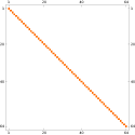
(a) $L^{2}$-scalar product of $B_{kl},C_{kl}$ and auxiliary functions.

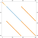
(b) $L^{2}$-scalar product of $B_{kl},C_{kl}$ and $H(\operatorname{curl})$ basis functions.

Figure 1: Biorthogonal sparsity pattern for $p=6$

For Section 4.2, we start with the biorthogonality condition. We again assume a tensorial-like structure, i.e. $C_{kl}(\eta,y)=c_{kl}^{(3)}(y)\begin{pmatrix}c_{k}^{(1)}(\eta)&c_{k}^{(2)}(\eta)\end{pmatrix}^{\top}$. The condition is

$$\langle\tilde{v}^{\triangle,II}_{ij}(\eta,y),C_{kl}(\eta,y)\rangle =\int_{-1}^{1}\widehat{L}_{i}(\eta)c_{k}^{(2)}(\eta)\,\mathrm{d}\eta\int_{-1}^{1}\left(\frac{1-y}{2}\right)^{i+1}P^{(2i,0)}_{j-1}(y)c_{kl}^{(3)}(y)\,\mathrm{d}y$$

$$=d^{(2)}_{ijkl}\delta_{ik}\delta_{jl}.$$

This leads to the choice $c_{k}^{(2)}(\eta)=\kappa P^{(1,1)}_{k-2}(\eta)$ and $c^{(3)}_{kl}(y)=\left(\frac{1-y}{2}\right)^{k-1}P^{(2k,0)}_{l-1}(y),$ where $\kappa$ is some constant. Condition $\langle\tilde{v}_{ij}^{\triangle,I},C_{kl}\rangle=0$ is satisfied, if $\langle\nabla f_{i}(\eta,y),C_{kl}(\eta)\rangle=0$. Since both components of $\nabla f_{i}$ depend on $\left(\frac{1-y}{2}\right)^{i-1}\widehat{P}_{j}^{2i,0}(y),$ the orthogonality relation reduces to

$$\int_{-1}^{1}L_{i-1}(\eta)c^{(1)}_{k}(\eta)\,\mathrm{d}\eta+\int_{-1}^{1}\frac{1}{2}L_{i-2}(\eta)c_{k}^{(2)}(\eta)\,\mathrm{d}\eta=0.$$

Due to lemma 4.8 this condition is fulfilled if $c_{k}^{(1)}(\eta)=(2+k-1)P_{k-1}^{(1,1)}(\eta)$
and ${c_{k}^{(2)}(\eta)=-2(2+k-2)P_{k-2}^{(1,1)}(\eta).}$ Now we have found biorthogonal functions for $\tilde{v}_{ij}^{\triangle,I}$ and $\tilde{v}_{ij}^{\triangle,II},$ which results in a diagonal matrix which can be seen in Figure 1(a).

Definition 4.10 (Dual functions on a triangle).

For $k\geq 2,l\geq 1$ define

(26) $$B_{kl}(x,y) \coloneqq\begin{pmatrix}L_{k-1}\left(\frac{2x}{1-y}\right)\left(\frac{1-y}{2}\right)^{k-1}P_{l-1}^{2k-1,1}(y)\\ 0\end{pmatrix},$$

$$C_{kl}(x,y) \coloneqq\begin{pmatrix}(2+k-1)P_{k-1}^{(1,1)}\left(\frac{2x}{1-y}\right)\left(\frac{1-y}{2}\right)^{k-1}P_{l-1}^{(2k,0)}(y)\\ -2(2+k-2)P_{k-2}^{(1,1)}\left(\frac{2x}{1-y}\right)\left(\frac{1-y}{2}\right)^{k-1}P_{l-1}^{(2k,0)}(y)\end{pmatrix}.$$

With this choice we have proven the following corollary.

Corollary 4.11.

Let $\tilde{v}^{\triangle,I}_{ij},\tilde{v}^{\triangle,II}_{ij}$ be defined by (23) and the functions $B_{kl}$ and $C_{kl}$ be defined as in Eq. 26. Then these functions are biorthogonal.

Obviously those are not biorthogonal to the basis $v^{\triangle,I}_{ij},v^{\triangle,II}_{ij}$ and $v^{\triangle,III}_{1j},$ which can be seen in Figure 1(b). Thus, we derive the biorthogonal functions by linear combination, as in the quadrilateral case.

Lemma 4.12.

Let $\alpha_{1}=\frac{1}{8}(2i-1)(2j+2i-1)(j+2i-1)$, $\alpha_{2}=\frac{1}{16}(2i-1)(2j+2i-1)$ and $\alpha_{3}=\frac{1}{16}(2j+2)(j+2)$. Then, for $2\leq i,k\leq p,1\leq j,l\leq p,$ and $i+j,k+l\leq p,$ the functions $v^{\triangle,I}_{ij},v^{\triangle,II}_{ij}$ and $v^{\triangle,III}_{1j}$ as in (21) are biorthogonal to

$$b^{\triangle,I}_{kl}(x,y) =-\frac{1}{2}(\alpha_{1}B_{kl}(x,y)+\alpha_{2}C_{kl}(x,y)),$$

$$b^{\triangle,II}_{kl}(x,y) =\frac{1}{2}(\alpha_{1}B_{kl}(x,y)-\alpha_{2}C_{kl}(x,y)),$$

$$b^{\triangle,III}_{1l}(x,y) =\alpha_{3}B_{1l}(x,y),$$

where $B_{kl}$ and $C_{kl}$ are given in Eq. 26.

Proof 4.13.

Since we have shown biorthogonality of $\tilde{v}_{ij}^{\triangle,I},\tilde{v}_{ij}^{\triangle,II}$ to $B_{kl},C_{kl}$ in Corollary 4.11, we get

$$\langle v^{\triangle,I}_{ij},B_{kl}\rangle=\langle\tilde{v}^{\triangle,I}_{ij},B_{kl}\rangle+\langle\tilde{v}^{\triangle,II}_{ij},B_{kl}\rangle=\langle\tilde{v}^{\triangle,I}_{ij},B_{kl}\rangle=c\delta_{ik}\delta_{jl}$$

$$\langle v^{\triangle,I}_{ij},C_{kl}\rangle=\langle\tilde{v}^{\triangle,I}_{ij},C_{kl}\rangle+\langle\tilde{v}^{\triangle,II}_{ij},C_{kl}\rangle=\langle\tilde{v}^{\triangle,II}_{ij},C_{kl}\rangle=\tilde{c}\delta_{ik}\delta_{jl}.$$

As in the quadrilateral case, lemma 4.4 with the matrix $A=\begin{bmatrix}1&1\\ 1&-1\end{bmatrix}$ is applied. For the diagonal matrix $D$ in this lemma, we have to compute $\langle\tilde{v}^{\triangle,I}_{ij},B_{ij}\rangle$ and $\langle\tilde{v}^{\triangle,II}_{ij},C_{ij}\rangle$ for $(i,j)=(k,l)$. Using (8) with $\alpha=\beta=0$ and $(\alpha,\beta)=(2i-1,0)$ one obtains

$$\langle\tilde{v}^{\triangle,I}_{ij},B_{ij}\rangle =\int_{-1}^{1}(L_{i-1}(\eta))^{2}\,\mathrm{d}\eta\int_{-1}^{1}\left(\frac{1-y}{2}\right)^{2i-1}\frac{(1+y)}{j}(P_{j-1}^{(2i-1,1)}(y))^{2}\,\mathrm{d}y$$

$$=\frac{8}{(2i-1)(2j+2i-1)(j+2i-1)}.$$

This gives $\alpha_{1}=\frac{1}{8}(2i-1)(2j-2i-1)(j+2i-1)$. Analogously (8) with $\alpha=\beta=1$ and $(\alpha,\beta)=(2i,0)$ gives

$$\langle\tilde{v}^{\triangle,II}_{ij},C_{ij}\rangle =-2i\int_{-1}^{1}\left(\frac{\eta^{2}-1}{2(i-1)}\right)(P^{(1,1)}_{i-2}(\eta))^{2}\,\mathrm{d}\eta\int_{-1}^{1}\left(\frac{1-y}{2}\right)^{2i}P^{(2i,0)}_{j-1}(y)\,\mathrm{d}y$$

$$=\frac{16}{(2i-1)(2j+2i-1)},$$

implies $\alpha_{2}=\frac{1}{16}(2i-1)(2j+2i-1).$ The only thing remaining to show is that $B_{kl},C_{kl}$ are orthogonal to $v^{\triangle,III}_{1,j}$ and that $b_{1l}^{\triangle,III}$ is orthogonal to $\tilde{v}^{\triangle,I}_{ij}$ and $\tilde{v}^{\triangle,II}_{ij}.$ Indeed,

$$\langle v^{\triangle,III}_{1j},B_{kl}\rangle=\int_{-1}^{1}1\cdot L_{k-1}(\eta)\,\mathrm{d}\eta\int_{-1}^{1}\frac{1}{2}\left(\frac{1-y}{2}\right)^{k}P_{l-1}^{(2k-1,1)}(y)=0,$$

due to the orthogonality of $L_{k-1}(\eta)$ for all $k\geq 2.$ For the orthogonality of $\langle v^{\triangle,III}_{1j},C_{kl}\rangle$. we can apply Lemma 4.8. On the other hand, orthogonality of $b_{1l}^{\triangle,III}$ follows from Corollary 4.11.

Since all basis functions are properly scaled, the next corollary follows directly.

Corollary 4.14.

Let $i,k\geq 2$ and $j,l\geq 1.$ Furthermore let $v^{\triangle,I}_{ij},v^{\triangle,II}_{ij},v^{\triangle,III}_{1j}$ be the basis of the $H(\operatorname{curl})$ interior functions and let $b^{\triangle,I}_{kl},b^{\triangle,II}_{kl},b^{\triangle,III}_{1l}$ be the corresponding normalized dual face functions, then holds for the entries of the element Matrix $G$ that

$$G_{ij,kl}=\langle v^{\triangle,T_{1}}_{ij}(x,y),b_{kl}^{\triangle,T_{2}}(x,y)\rangle=\delta_{i,k}\delta_{j,l}\delta_{T_{1},T_{2}}.$$

4.3 Tetrahedral case

Our ansatz is the same as in the triangular case. Firstly, we split the basis functions in a simpler basis, then find the orthogonal basis to this simpler basis, and lastly build the right dual basis by linear combination. Recall the basis of $H(\operatorname{curl})$ on the tetrahedral $\blacktriangle$ is given by

(27) $$v_{ijk}^{I} =\nabla(f_{i}g_{ij}h_{ijk})=\nabla(f_{i})g_{ij}h_{ijk}+f_{i}\nabla(g_{ij})h_{ijk}+f_{i}g_{ij}\nabla(h_{ijk}),$$

$$v_{ijk}^{II} =\nabla(f_{i})g_{ij}h_{ijk}-f_{i}\nabla(g_{ij})h_{ijk}+f_{i}g_{ij}\nabla(h_{ijk}),$$

$$v_{ijk}^{III} =\nabla(f_{i})g_{ij}h_{ijk}+f_{i}\nabla(g_{ij})h_{ijk}-f_{i}g_{ij}\nabla(h_{ijk}),$$

$$v_{1jk}^{IV} =v^{\mathcal{N}_{0}}_{[1,2]}g_{ij}h_{ijk},$$

for $2\leq i,1\leq j,k,$ and $i+j+k\leq p,$ where $f_{i}(x,y,z)=\widehat{L}_{i}\left(\frac{4x}{1-2y-z}\right)\left(\frac{1-2y-z}{4}\right)^{i}$, $g_{ij}(y,z)=\widehat{P}_{j}^{2i}\left(\frac{2y}{1-z}\right)\left(\frac{1-z}{2}\right)^{j},$ and $h_{ijk}(z)=\widehat{P}_{k}^{2i+2j}(z).$ Here $v_{[1,2]}^{\mathcal{N}_{0}}$ is the lowest order Nédélec function of first kind, based on the edge from vertex $1$ to $2$. With the substitutions $\eta=\frac{4x}{1-2y-z}$ and $\chi=\frac{2y}{1-z},$ the gradients of the auxiliary functions are

$$\nabla f_{i} =\begin{pmatrix}L_{i-1}(\eta)\\ \frac{1}{2}L_{i-2}(\eta)\\ \frac{1}{4}L_{i-2}(\eta)\end{pmatrix}\left(\frac{1-\chi}{2}\right)^{i-1}\left(\frac{1-z}{2}\right)^{i-1},$$

$$\nabla g_{ij} =\begin{pmatrix}0\\ P_{j-1}^{(2i,0)}(\chi)\\ \frac{\chi}{2}P_{j-1}^{(2i,0)}(\chi)-\frac{j}{2}\widehat{P}_{j}^{2i}(\chi)\end{pmatrix}\left(\frac{1-z}{2}\right)^{j-1}\text{ and }$$

$$\nabla h_{ijk} =\begin{pmatrix}0\\ 0\\ P^{(2i+2j,0)}_{k-1}(z)\end{pmatrix},$$

with the simplifications as in [11, 7]. We now derive three biorthogonal vectors with respect to $(\nabla f_{i})\,g_{ij}\,h_{ijk},f_{i}\,(\nabla g_{ij})\,h_{ijk}$ and $f_{i}\,g_{ij}\,(\nabla h_{ijk}).$
Similar to the triangular case, we have the following conditions on the dual functions $B_{ijk},C_{ijk}$ and $D_{ijk}:$ Find $B_{lmn},C_{lmn},D_{lmn}$ such that

$$f_{i}\,(\nabla g_{ij})\,h_{ijk}\perp B_{lmn}\perp f_{i}\,g_{ij}\,(\nabla h_{ijk})\text{ and }\langle B_{lmn},(\nabla f_{i})\,g_{ij}\,h_{ijk}\rangle=r_{ijklmn}\delta_{il}\delta_{jm}\delta_{kn},$$

$$(\nabla f_{i})\,g_{ij}\,h_{ijk}\perp C_{lmn}\perp f_{i}\,g_{ij}\,(\nabla h_{ijk})\text{ and }\langle C_{lmn},f_{i}\,(\nabla g_{ij})\,h_{ijk}\rangle=s_{ijklmn}\delta_{il}\delta_{jm}\delta_{kn},$$

$$(\nabla f_{i})\,g_{ij}\,h_{ijk}\perp D_{lmn}\perp f_{i}\,(\nabla g_{ij})\,h_{ijk}\text{ and }\langle D_{lmn},f_{i}\,g_{ij}\,(\nabla h_{ijk})\rangle=t_{ijklmn}\delta_{il}\delta_{jm}\delta_{kn}.$$

Since the basis vectors build a lower triangular system, we know that we need to find an upper triangular system. Thus,

$$B_{lmn}=\begin{pmatrix}b_{lmn}(\eta,\chi,z)\\ 0\\ 0\end{pmatrix},\quad C_{lmn}=\begin{pmatrix}c^{(1)}_{lmn}(\eta,\chi,z)\\ c^{(2)}_{lmn}(\eta,\chi,z)\\ 0\end{pmatrix},\quad\textrm{and}\quad D_{lmn}=\begin{pmatrix}d^{(1)}_{lmn}(\eta,\chi,z)\\ d^{(2)}_{lmn}(\eta,\chi,z)\\ d^{(3)}_{lmn}(\eta,\chi,z)\end{pmatrix}.$$

The construction of $B_{lmn}$ is trivial, and the construction of $C_{lmn}$ follows from the $2D$ case. Thus,

$$B_{lmn} =\begin{pmatrix}1\\ 0\\ 0\end{pmatrix}L_{l-1}(\eta)\left(\frac{1-\chi}{2}\right)^{l-1}P_{m-1}^{(2l-1,1)}(\chi)\left(\frac{1-z}{2}\right)^{l+m-2}P_{n-1}^{(2l+2m-1,1)}(z)\text{ and }$$

$$C_{lmn} =\begin{pmatrix}(2+l-1)P^{(1,1)}_{l-1}(\eta)\\ -2(2+l-2)P^{(1,1)}_{l-2}(\eta)\\ 0\end{pmatrix}\left(\frac{1-\chi}{2}\right)^{l-1}P_{m-1}^{(2l,0)}(\chi)\left(\frac{1-z}{2}\right)^{l+m-2}P_{n-1}^{(2l+2m-1,1)}(z),$$

where the exponents of $\left(\frac{1-\chi}{2}\right)$ and $\left(\frac{1-z}{2}\right)$ are determined with respect to the functional determinant of the Duffy trick, i.e. $\left(\frac{1-\chi}{2}\right)\left(\frac{1-z}{2}\right)^{2}.$
To derive $D_{lmn},$ we go step by step. It follows immediately that

(28) $$d^{(3)}_{lmn}=P_{l-2}^{(1,1)}(\eta)\left(\frac{1-\chi}{2}\right)^{l-2}P_{m-1}^{(2l-1,1)}(\chi)\left(\frac{1-z}{2}\right)^{l+m-2}P_{n-1}^{(2l+2m,0)}(z),$$

due to $\langle D_{lmn},f_{i}\,g_{ij}\,(\nabla h_{ijk})\rangle=s_{ijklmn}\delta_{il}\delta_{jm}\delta_{kn}.$ Next we derive $d^{(2)}_{lmn}$ by demanding

(29) $$0=\langle f_{i}(\nabla g_{ij})h_{ijk},D_{lmn}\rangle.$$

An rather obvious choice for $d^{(2)}_{lmn}$ is $d^{(2)}_{lmn}=P^{(1,1)}_{l-2}(\eta)\,\tilde{d}^{(2)}(\chi)\left(\frac{1-z}{2}\right)^{l+m-2}P_{n-1}^{(2l+2m,0)}(z).$ This choice reduces the condition (29) to

(30) $$0= \int_{-1}^{1}\left(\frac{1-\chi}{2}\right)^{i+1}P_{j-1}^{(2i,0)}(\chi)\,\tilde{d}^{(2)}(\chi)$$

$$+\left(\frac{1-\chi}{2}\right)^{2i-1}\left(\frac{\chi}{2}P_{j-1}^{(2i,0)}(\chi)-\frac{j}{2}\widehat{P}_{j}^{2i}(\chi)\right)P_{m-1}^{(2i-1,1)}(\chi)\,\mathrm{d}\chi,$$

since the condition (29) is trivial for $i\neq l$ and $k\neq n$ with this choice of $d^{(2)}_{ijk}.$
On the right part of the integral, the combination $\widehat{P}^{2i}_{j}(\chi)P_{m-1}^{(2i-1,1)}(\chi)$ already fulfils the orthogonality relation. On the other hand, for the product of the two different Jacobi polynomials, namely $P^{(2i,0)}_{j-1}(\chi)$ and $P_{m-1}^{(2i-1,1)}(\chi),$ we can’t apply standard orthogonality results. We eliminate this mixed part by linear combination. Therefore, we choose

$$\tilde{d}^{(2)}=-\frac{\chi}{2}\left(\frac{1-\chi}{2}\right)^{l-2}P_{m-1}^{(2l-1,1)}(\chi)+\hat{d}^{(2)},$$

such that the mixed products cancel each other out. Those linear combinations result in the further reduced condition

(31) $$0=\int_{-1}^{1}\left(\frac{1-\chi}{2}\right)^{i+1}P_{j-1}^{(2i,0)}(\chi)\,\hat{d}^{(2)}(\chi)-\frac{j}{2}\left(\frac{1-\chi}{2}\right)^{2i-1}\widehat{P}_{j}^{2i}(\chi)P_{m-1}^{(2i-1,1)}(\chi)\,\mathrm{d}\chi.$$

The last part of the integral in (31) only appears if $m=j.$ We can achieve the same for the first part of the integral, if we choose $\hat{d}^{(2)}=c\left(\frac{1-\chi}{2}\right)^{l-1}P_{m-1}^{(2l,0)}(\chi)$. Since both instances in (31) are integrals over Jacobi polynomials with matching indices, order and weights, we can determine the constant $c$ directly. It holds that

$$\int_{-1}^{1}\left(\frac{1-\chi}{2}\right)^{2i}\left(P_{j-1}^{(2i,0)}(\chi)\right)^{2}\,\mathrm{d}\chi =\frac{1}{2j+2i-1}$$

$$\int_{-1}^{1}\left(\frac{1-\chi}{2}\right)^{2i-1}\left(\frac{1+\chi}{2}\right)\left(P_{j-1}^{(2i-1,1)}(\chi)\right)^{2}\,\mathrm{d}\chi =\frac{j}{(2j+2i-1)(2i+j-1)}.$$

Collecting everything

$$d^{(2)}_{lmn}=P^{(1,1)}_{l-2}(\eta) \left(\frac{1-\chi}{2}\right)^{l-2}Q_{m,2}(\chi)\left(\frac{1-z}{2}\right)^{l+m-2}P_{n-1}^{(2l+2m,0)}(z)$$

with the polynomial

(32) $$Q_{m,2}(\chi)=-\frac{\chi}{2}P_{m-1}^{(2l-1,1)}(\chi)+\frac{m}{2l+m-1}\frac{1-\chi}{2}P_{m-1}^{(2l,0)}(\chi)$$

of degree $m$. Now we need to determine $d^{(1)}_{lmn},$ by $0=\langle(\nabla f_{i})g_{ij}h_{ijk},D_{lmn}\rangle$. Inserting $d^{(2)}_{lmn}$ and $d^{(3)}_{lmn}$ yields the following condition, after some simplification

$$0= \int_{(-1,1)^{3}}L_{i-1}(\eta)\left(\frac{1-\chi}{2}\right)^{i-1}\widehat{P}_{j}^{2i}(\chi)\left(\frac{1-z}{2}\right)^{i+j+1}\widehat{P}^{2i+2j}_{k}(z)d^{(1)}_{lmn}(\eta,\chi,z)\,\mathrm{d}\eta\,\mathrm{d}\chi\,\mathrm{d}z$$

$$+\int_{(-1,1)^{3}}L_{i-2}(\eta)P_{l-2}^{(1,1)}(\eta)\left(\frac{1-\chi}{2}\right)^{i+l-1}\widehat{P}^{2i}_{j}(\chi)\left[P_{m-1}^{(2l-1,1)}(\chi)+\frac{m}{2l+m-1}P_{m-1}^{(2l,0)}(\chi)\right]$$

$$\left(\frac{1-z}{2}\right)^{i+j+l+m-1}\widehat{P}^{2i+2j}_{k}(z)P^{(2l+2m-1,1)}_{n-1}(z)\,\mathrm{d}z\,\mathrm{d}\chi\,\mathrm{d}\eta.$$

If we choose $d^{(1)}_{lmn}(\eta,\chi,z)=\frac{2+l-1}{2(2+l-2)}P_{l-1}^{(1,1)}(\eta)\hat{d}^{(1)}(\chi)\left(\frac{1-z}{2}\right)^{l+m-2}P_{n-1}^{(2l+2m,0)}(z),$ we can factor all terms depending on $\eta$ and $z$ out. Thus, we only need to determine $\hat{d}^{(1)}(\chi),$ by the condition

$$0= \int_{-1}^{1}\left(\frac{1-\chi}{2}\right)^{i-1}\widehat{P}_{j}^{2i}(\chi)\,\hat{d}^{(1)}(\chi)$$

$$+\left(\frac{1-\chi}{2}\right)^{i+l-1}\widehat{P}^{2i}_{j}(\chi)\left[P_{m-1}^{(2l-1,1)}(\chi)+\frac{m}{2l+m-1}P_{m-1}^{(2l,0)}(\chi)\right]\,\mathrm{d}\chi.$$

It is obvious, that we can choose

$$d^{(1)}_{lmn}= \frac{-(2+l-1)}{2(2+l-2)}P_{l-1}^{(1,1)}(\eta)\left(\frac{1-\chi}{2}\right)^{l-1}Q_{m-1,1}(\chi)\left(\frac{1-z}{2}\right)^{l+m-2}P_{n-1}^{(2l+2m,0)}(z)$$

with the $m-1$ degree polynomial

(33) $$Q_{m-1,1}(\chi)=P_{m-1}^{(2l-1,1)}(\chi)+\frac{m}{2l+m-1}P_{m-1}^{(2l,0)}(\chi).$$

We summarize in the following definition.

Definition 4.15 (Dual basis on the tetrahedron).

Let $Q_{m-1,1}$ and $Q_{m,2}$ be defined by (33) and (32), respectively. Let $l\geq 2,m,n\geq 1$ then define

(34) $$\tilde{b}^{\blacktriangle,I}_{lmn}\coloneqq \begin{pmatrix}1\\ 0\\ 0\end{pmatrix}L_{l-1}(\eta)\left(\frac{1-\chi}{2}\right)^{l-1}P_{m-1}^{(2l-1,1)}(\chi)\left(\frac{1-z}{2}\right)^{l+m-2}P_{n-1}^{(2l+2m-1,1)}(z)$$

$$\tilde{b}^{\blacktriangle,II}_{lmn}\coloneqq \begin{pmatrix}(l+1)P^{(1,1)}_{l-1}(\eta)\\ -2lP^{(1,1)}_{l-2}(\eta)\\ 0\end{pmatrix}\left(\frac{1-\chi}{2}\right)^{l-1}P_{m-1}^{(2l,0)}(\chi)\left(\frac{1-z}{2}\right)^{l+m-2}P_{n-1}^{(2l+2m-1,1)}(z),$$

$$\tilde{b}^{\blacktriangle,III}_{lmn}\coloneqq \begin{pmatrix}\frac{-(l+1)}{2\,l}P_{l-1}^{(1,1)}(\eta)\left(\frac{1-\chi}{2}\right)^{l-1}Q_{m-1,1}(\chi)\\ P_{l-2}^{(1,1)}(\eta)\left(\frac{1-\chi}{2}\right)^{l-2}Q_{m,2}(\chi)\\ P_{l-2}^{(1,1)}(\eta)\left(\frac{1-\chi}{2}\right)^{l-2}P_{m-1}^{(2l-1,1)}(\chi)\end{pmatrix}\left(\frac{1-z}{2}\right)^{l+m-2}P_{n-1}^{(2l+2m,0)}(z),$$

where $\eta=\frac{4x}{1-2y-z}$, $\chi=\frac{1-2y-z}{4}$ .

Thus, the following lemma has been shown.

Lemma 4.16.

Let $f_{i},g_{ij}$ and $h_{ijk}$ be defined as in (27). Then, the functions

$$\tilde{v}^{\blacktriangle,I}_{ijk}=(\nabla f_{i})g_{ij}h_{ijk},\quad\tilde{v}^{\blacktriangle,II}_{ijk}=f_{i}(\nabla g_{ij})h_{ijk},\quad\textrm{and}\quad\tilde{v}^{\blacktriangle,III}_{ijk}=f_{i}g_{ij}(\nabla h_{ijk})$$

are biorthogonal to $\tilde{b}_{lmn}^{\blacktriangle,I},\tilde{b}_{lmn}^{\blacktriangle,II}$ and $\tilde{b}_{lmn}^{\blacktriangle,III}$ defined by Eq. 34, i.e.

$$\langle\tilde{v}^{\blacktriangle,\omega_{1}}_{ijk},\tilde{b}^{\blacktriangle,\omega_{2}}_{lmn}\rangle=c^{\omega_{1}}_{ijk}\,\delta_{il}\delta_{jm}\delta_{kn}\delta_{\omega_{1},\omega_{2}},\quad\omega_{1},\omega_{2}\in\{I,II,III\}.$$

As before, we transfer this to the original interior basis functions.

Lemma 4.17.

Let $\tilde{b}_{lmn}^{\blacktriangle,I},\tilde{b}_{lmn}^{\blacktriangle,I}$ and $\tilde{b}_{lmn}^{\blacktriangle,I}$ be defined by Eq. 34.
For $i\geq 2,j\geq 1,k\geq 1$ the functions $v^{\blacktriangle,I}_{ijk},v^{\blacktriangle,II}_{ijk},v^{\blacktriangle,III}_{ijk}$ and $v^{\blacktriangle,IV}_{1jk}$ are biorthogonal to

$$b^{\blacktriangle,I}_{lmn} =\frac{1}{2}\alpha^{(2)}_{lmn}\tilde{b}^{\blacktriangle,II}_{lmn}+\frac{1}{2}\alpha^{(3)}_{lmn}\tilde{b}^{\blacktriangle,III}_{lmn},$$

$$b^{\blacktriangle,II}_{lmn} =\frac{1}{2}\alpha^{(1)}_{lmn}\tilde{b}^{\blacktriangle,I}_{lmn}-\frac{1}{2}\alpha_{lmn}^{(2)}\tilde{b}^{\blacktriangle,II}_{lmn},$$

$$b^{\blacktriangle,III}_{lmn} =\frac{1}{2}\alpha^{(1)}_{lmn}\tilde{b}^{\blacktriangle,I}_{lmn}-\frac{1}{2}\alpha_{lmn}^{(3)}\tilde{b}^{\blacktriangle,III}_{lmn},$$

$$b^{\blacktriangle,IV}_{1mn} =\alpha^{(4)}_{lmn}\tilde{b}^{\blacktriangle,I}_{1mn},$$

where

$$\alpha^{(1)}_{lmn} =\frac{1}{2^{7}}(2l-1)(2m+2l-1)(m+2l-1)(2n+2l+2m-1)(n+2l+2m-1)$$

$$\alpha^{(2)}_{lmn} =\frac{1}{2^{6}}(2l-1)(2m+2l-1)(2n+2l+2m-1)(n+2l+2m-1)$$

$$\alpha^{(3)}_{lmn} =\frac{-1}{2^{5}}l(2l-1)(2m+2l-1)(m+2l-1)(2n+2l+2m-1)$$

$$\alpha^{(4)}_{lmn} =\frac{1}{2^{5}}(2m+2)(m+2)(n+2m+2)(2n+2m+2)$$

Proof 4.18.

Again, we apply Lemma 4.4. Now, $A=\begin{bmatrix}1&1&1\\ 1&-1&1\\ 1&1&-1\end{bmatrix}$. from which its inverse is easily be computed as $A^{-1}=\frac{1}{2}\begin{bmatrix}0&1&1\\ 1&-1&0\\ 1&0&-1\end{bmatrix}$. It remains to compute the diagonal entries.

The coefficients $c^{\omega}_{ijk}$ can be computed analogously to the triangular case be using the exact values of the integrals over Jacobi polynomials. Finally, one obtains

$$\langle\tilde{v}_{ijk}^{I},\tilde{b}_{ijk}^{I}\rangle =\frac{2^{7}}{(2i-1)}\frac{1}{(2j+2i-1)(j+2i-1)(2k+2i+2j-1)(k+2i+2j-1)},$$

$$\langle\tilde{v}_{ijk}^{II},\tilde{b}_{ijk}^{II}\rangle =\frac{2^{6}}{(2i-1)}\frac{1}{(2j+2i-1)(2k+2i+2j-1)(k+2i+2j-1)},$$

$$\langle\tilde{v}_{ijk}^{III},\tilde{b}_{ijk}^{III}\rangle =\frac{2^{6}}{(2i-1)}\frac{1}{i\,(2i+2j-1)(j+2i-1)(2k+2i+2j-1)},$$

by using the orthogonality relations of the Jacobi polynomials (8). It remains to show, that to

$$v^{IV}_{1jk}=\begin{pmatrix}1\\ \frac{\eta}{2}\\ \frac{\eta}{4}\end{pmatrix}\left(\frac{1-\chi}{2}\right)\widehat{P}^{1}_{j}(\chi)\left(\frac{1-z}{2}\right)^{j+1}\widehat{P}^{2j+3}_{k}(z)$$

the dual shape functions are naturally orthogonal. For $B_{ijk}$ orthogonality follows since the first component of $v^{IV}_{1jk}$ is independent of $\eta=\frac{4x}{1-2y-z}.$
For $C_{ijk}$ we apply the relations

$$\int_{-1}^{1}(i+1)P^{(1,1)}_{i-1}(x)\,\mathrm{d}x =2\int_{-1}^{1}\frac{\mathrm{d}}{\mathrm{d}x}L_{i}(x)\,\mathrm{d}x=2\left[L_{i}(x)\right]_{-1}^{1}=2(1-(-1)^{i})\quad\textrm{and}$$

$$\int_{-1}^{1}\frac{x}{2}(2i)P^{(1,1)}_{i-2}(x)\,\mathrm{d}x =2\int_{-1}^{1}x\frac{\mathrm{d}}{\,\mathrm{d}x}L_{i-1}(x)\,\mathrm{d}x$$

$$=2\left[xL_{i}(x)\right]_{-1}^{1}-\underbrace{\int_{-1}^{1}L_{-1}(x)}_{=0}\,\mathrm{d}x=2(1-(-1)^{i})$$

to see that the scalar product $\langle v^{IV}_{1jk},C_{lmn}\rangle=0,$ for all $i,j,k,l,m,n.$ For $D_{ijk}$ the same relation is applied, thus $\langle v^{IV}_{1jk},D_{lmn}\rangle=0,$ for all $i,j,k,l,m,n.$ On the other hand the dual function to $v^{IV}_{1jk}$ is easily found to be $B_{1jk}=\begin{pmatrix}1\\ 0\\ 0\end{pmatrix}P_{j-1}^{(2,1)}(y)\left(\frac{1-z}{2}\right)^{j-1}P_{k-1}^{(2j+2,1)}(z)$. It is obviously orthogonal to $\nabla g_{ij}$ and $\nabla h_{ijk},$ furthermore it is orthogonal to $\nabla f_{i}$ since it is independent of $\eta.$

We conclude with some remarks.

Remark 4.19.

It is usually possible to modify the index of the integrated Jacobi polynomials to modify the sparsity pattern and condition number of the element matrices. But in the context of polynomial dual functions the index $(2i)$ and $(2i+2j)$ are minimal, otherwise the dual functions will become rational with singularities for low polynomial degrees for the interior $H(\operatorname{curl})$ shape functions.

Remark 4.20.

The coefficients $\alpha_{lmn}^{(1)},\alpha_{lmn}^{(2)}$ and $\alpha_{lmn}^{(3)}$ can be significantly reduced by dividing each with

$$(2l\scalebox{0.65}[1.0]{$+$}2m\scalebox{0.65}[1.0]{$-$}1)(2l\scalebox{0.65}[1.0]{$-$}1)(2n\scalebox{0.65}[1.0]{$-$}2l\scalebox{0.65}[1.0]{$-$}2m\scalebox{0.65}[1.0]{$-$}1).$$

In this case one needs to compute the element matrix corresponding to biorthogonal system by numerical quadrature or similar methods.

5 Conclusion

We summarize the main contribution of this paper in a more abstract notation. Let $\mathbb{V}_{0}$ be the space $H^{1}_{0}$ or $H_{0}(\operatorname{curl})$ on an element $\Omega$ and $\mathbb{V}_{hp,0}=\mathbb{V}_{hp}\cap\mathbb{V}_{0}$. For given element based families of $hp$-FEM basis functions $\phi_{i}\in\mathbb{V}_{hp,0},$ the authors developed biorthogonal test functions $\psi_{j}\in W_{hp}$. This allows us to represent the $L^{2}$-like projection based interpolation operator $\mathcal{P}:\mathbb{V}_{0}(\Omega)\mapsto\mathbb{V}_{hp,0}$ given by

$$\int_{\Omega}(\mathcal{P}u)(\vec{x})\;v_{hp}(\vec{x})(\vec{x})\;\mathrm{d}\vec{x}=\int_{\Omega}u(\vec{x})v_{hp}(\vec{x})\;\mathrm{d}\vec{x}\quad\forall v_{hp}\in W_{hp}.$$

by

$$(Pu)(\vec{x})=\sum_{i}\phi_{i}(\vec{x})g_{i}\quad\textrm{with}\quad g_{i}=\int_{\Omega}u(\vec{x})\psi_{i}(\vec{x})\;\mathrm{d}\vec{x}.$$

The primal functions $\phi_{i}$ are basis functions which are optimal to sparsity and condition number on the reference element. The dual functions are expressed in closed expressions in terms of Jacobi polynomials. This result can be used for further results in error estimation and preconditioning where the above-mentioned operator $\mathcal{P}$ is used.
An extension to other weights or indices of Jacobi polynomials is limited. Since we include the weights of Jacobi polynomials in the basis functions, a decrease in the related indices results in the loss of most orthogonality relations for the low order cases. On the other hand, an increase of the indices results in a modification of the dual functions and in a higher polynomial test space in (3). From the point of view of the authors, closed formulas for dual functions of the basis functions of Fuentes et al. [17] are very ambitious to develop.

6 Acknowledgment

References

- [1] M. Ainsworth, G. Andriamaro, and O. Davydov, Bernstein-Bézier finite elements of arbitrary order and optimal assembly procedures, SIAM J. Sci. Comput., 33 (2011), pp. 3087–3109, https://doi.org/10.1137/11082539X, https://doi.org/10.1137/11082539X.
- [2] M. Ainsworth and J. Coyle, Hierarchic hp-edge element families for maxwell’s equations on hybrid quadrilateral/triangular meshes, Computer Methods in Applied Mechanics and Engineering, 190 (2001), pp. 6709–6733, https://doi.org/https://doi.org/10.1016/S0045-7825(01)00259-6, https://www.sciencedirect.com/science/article/pii/S0045782501002596.
- [3] M. Ainsworth and G. Fu, Bernstein-Bézier bases for tetrahedral finite elements, Comput. Methods Appl. Mech. Engrg., 340 (2018), pp. 178–201, https://doi.org/10.1016/j.cma.2018.05.034, https://doi.org/10.1016/j.cma.2018.05.034.
- [4] G. E. Andrews, R. Askey, and R. Roy, Special functions, vol. 71 of Encyclopedia of Mathematics and its Applications, Cambridge University Press, Cambridge, 1999, https://doi.org/10.1017/CBO9781107325937, https://doi.org/10.1017/CBO9781107325937.
- [5] I. Babuška, M. Griebel, and J. Pitkäranta, The problem of selecting the shape functions for ap-type finite element, International Journal for Numerical Methods in Engineering, 28 (1989), pp. 1891–1908, https://doi.org/10.1002/nme.1620280813, https://doi.org/10.1002/nme.1620280813.
- [6] S. Beuchler and V. Pillwein, Sparse shape functions for tetrahedral -FEM using integrated Jacobi polynomials, Computing, 80 (2007), pp. 345–375, https://doi.org/10.1007/s00607-007-0236-0, https://doi.org/10.1007/s00607-007-0236-0.
- [7] S. Beuchler and V. Pillwein, Completions to sparse shape functions for triangular and tetrahedral -FEM, in Domain decomposition methods in science and engineering XVII, vol. 60 of Lect. Notes Comput. Sci. Eng., Springer, Berlin, 2008, pp. 435–442, https://doi.org/10.1007/978-3-540-75199-1_55, https://doi.org/10.1007/978-3-540-75199-1_55.
- [8] S. Beuchler, V. Pillwein, J. Schöberl, and S. Zaglmayr, Sparsity optimized high order finite element functions on simplices, in Numerical and symbolic scientific computing, Texts Monogr. Symbol. Comput., SpringerWienNewYork, Vienna, 2012, pp. 21–44, https://doi.org/10.1007/978-3-7091-0794-2_2, https://doi.org/10.1007/978-3-7091-0794-2_2.
- [9] S. Beuchler, V. Pillwein, and S. Zaglmayr, Sparsity optimized high order finite element functions for h(div) on simplices, Numerische Mathematik, 122 (2012), p. 197–225, https://doi.org/https://doi.org/10.1007/s00211-012-0461-010.1007/s00211-012-0461-0.
- [10] S. Beuchler, V. Pillwein, and S. Zaglmayr, Sparsity optimized high order finite element functions for h(curl) on tetrahedra, Advances in Applied Mathematics, 50 (2013), pp. 749–769, https://doi.org/https://doi.org/10.1016/j.aam.2012.11.004, https://www.sciencedirect.com/science/article/pii/S0196885812001303.
- [11] S. Beuchler and J. Schöberl, New shape functions for triangular -FEM using integrated Jacobi polynomials, Numer. Math., 103 (2006), pp. 339–366, https://doi.org/10.1007/s00211-006-0681-2, https://doi.org/10.1007/s00211-006-0681-2.
- [12] L. Demkowicz, Computing with hp-ADAPTIVE FINITE ELEMENTS: Volume 1 One and Two Dimensional Elliptic and Maxwell Problems, Chapman & Hall/CRC Applied Mathematics & Nonlinear Science, CRC Press, 2006, https://books.google.de/books?id=JwbOBQAAQBAJ.
- [13] L. Demkowicz, J. Kurtz, D. Pardo, M. Paszyński, W. Rachowicz, and A. Zdunek, Computing with -adaptive finite elements. Vol. 2, Chapman & Hall/CRC Applied Mathematics and Nonlinear Science Series, Chapman & Hall/CRC, Boca Raton, FL, 2008. Frontiers: three dimensional elliptic and Maxwell problems with applications.
- [14] M. Dubiner, Spectral methods on triangles and other domains, J. Sci. Comput., 6 (1991), pp. 345–390, https://doi.org/10.1007/BF01060030, https://doi.org/10.1007/BF01060030.
- [15] C. F. Dunkl and Y. Xu, Orthogonal polynomials of several variables, vol. 155 of Encyclopedia of Mathematics and its Applications, Cambridge University Press, Cambridge, second ed., 2014, https://doi.org/10.1017/CBO9781107786134, https://doi.org/10.1017/CBO9781107786134.
- [16] T. Eibner and J. Melenk, Fast algorithms for setting up the stiffness matrix in hp-fem: a comparison, Preprintreihe des Chemnitzer SFB 393, 05-08, (2005), pp. 1–39, https://nbn-resolving.org/urn:nbn:de:swb:ch1-200601623.
- [17] F. Fuentes, B. Keith, L. Demkowicz, and S. Nagaraj, Orientation embedded high order shape functions for the exact sequence elements of all shapes, Comput. Math. Appl., 70 (2015), pp. 353–458, https://doi.org/10.1016/j.camwa.2015.04.027, https://doi.org/10.1016/j.camwa.2015.04.027.
- [18] J. Gopalakrishnan, L. García-Castillo, and L. Demkowicz, Nédélec spaces in affine coordinates, Computers & Mathematics with Applications, 49 (2005), pp. 1285–1294, https://doi.org/10.1016/j.camwa.2004.02.012, https://doi.org/10.1016/j.camwa.2004.02.012.
- [19] T. Haubold, V. Pillwein, and S. Beuchler, Symbolic Evaluation of hp‐FEM Element Matrices, PAMM, 19 (2019), https://doi.org/10.1002/pamm.201900446.
- [20] G. E. Karniadakis and S. J. Sherwin, Spectral/ element methods for CFD, Numerical Mathematics and Scientific Computation, Oxford University Press, Oxford, second ed., 2013.
- [21] J.-F. Maitre and O. Pourquier, Condition number and diagonal preconditioning: comparison of the -version and the spectral element methods, Numer. Math., 74 (1996), pp. 69–84, https://doi.org/10.1007/s002110050208, https://doi.org/10.1007/s002110050208.
- [22] S. Mallat, A Wavelet Tour of Signal Processing, Elsevier, 2009, https://doi.org/10.1016/b978-0-12-374370-1.x0001-8, https://doi.org/10.1016/b978-0-12-374370-1.x0001-8.
- [23] J. Melenk, Hp-Finite Element Methods for Singular Perturbations, no. Nr. 1796 in Hp-finite Element Methods for Singular Perturbations, Springer, 2002, https://books.google.de/books?id=d1X-OaHrZxUC.
- [24] P. Monk, Finite Element Methods for Maxwell’s Equations, Numerical Mathematics and Scie, Clarendon Press, 2003, https://books.google.de/books?id=zI7Y1jT9pCwC.
- [25] J. Schöberl, C++11 implementation of finite elements in ngsolve, 09 2014.
- [26] C. Schwab, - and -finite element methods, Numerical Mathematics and Scientific Computation, The Clarendon Press, Oxford University Press, New York, 1998. Theory and applications in solid and fluid mechanics.
- [27] S. J. Sherwin and G. E. Karniadakis, A new triangular and tetrahedral basis for high-order finite element methods, Internat. J. Numer. Methods Engrg., 38 (1995), pp. 3775–3802, https://doi.org/10.1002/nme.1620382204, https://doi.org/10.1002/nme.1620382204.
- [28] B. Szabó and I. Babuška, Finite element analysis, A Wiley-Interscience Publication, John Wiley & Sons, Inc., New York, 1991.
- [29] G. Szegő, Orthogonal polynomials, American Mathematical Society, Providence, R.I., third ed., 1967. American Mathematical Society Colloquium Publications, Vol. 23.
- [30] C. Wieners and B. I. Wohlmuth, The coupling of mixed and conforming finite element discretizations, in Domain decomposition methods, 10 (Boulder, CO, 1997), vol. 218 of Contemp. Math., Amer. Math. Soc., Providence, RI, 1998, pp. 547–554, https://doi.org/10.1090/conm/218/03055, https://doi.org/10.1090/conm/218/03055.
- [31] B. I. Wohlmuth and R. H. Krause, A multigrid method based on the unconstrained product space for mortar finite element discretizations, SIAM Journal on Numerical Analysis, 39 (2001), pp. 192–213, https://doi.org/10.1137/S0036142999360676, https://doi.org/10.1137/S0036142999360676, https://arxiv.org/abs/https://doi.org/10.1137/S0036142999360676.
- [32] S. Zaglmayr, High Order Finite Elements for Electromagnetic Field Computation, PhD thesis, Johannes Kepler University Linz, 07 2006.