Leveraging Neural Radiance Fields for Uncertainty-Aware Visual Localization

Abstract

As a promising fashion for visual localization, scene coordinate regression (SCR) has seen tremendous progress in the past decade. Most recent methods usually adopt neural networks to learn the mapping from image pixels to 3D scene coordinates, which requires a vast amount of annotated training data. We propose to leverage Neural Radiance Fields (NeRF) to generate training samples for SCR. Despite NeRF’s efficiency in rendering, many of the rendered data are polluted by artifacts or only contain minimal information gain, which can hinder the regression accuracy or bring unnecessary computational costs with redundant data. These challenges are addressed in three folds in this paper: (1) A NeRF is designed to separately predict uncertainties for the rendered color and depth images, which reveal data reliability at the pixel level. (2) SCR is formulated as deep evidential learning with epistemic uncertainty, which is used to evaluate information gain and scene coordinate quality. (3) Based on the three arts of uncertainties, a novel view selection policy is formed that significantly improves data efficiency. Experiments on public datasets demonstrate that our method could select the samples that bring the most information gain and promote the performance with the highest efficiency.

I INTRODUCTION

Visual localization, which addresses the problem of estimating the camera pose of a query image in a known environment, is a key component in many robotics applications. One way to tackle it is through correspondences between image pixels and 3D map points, which can be obtained by Structure from Motion (SfM) and matching the sparse landmarks to image features. Another popular option is scene coordinate regression (SCR) which directly predicts pixelwise scene coordinates. Empowered by deep learning, recent methods of this category have achieved state-of-the-art performances in small or medium scale scenes [1, 2, 3]. Nevertheless, major challenges remain: (1) obtaining 2D-3D ground truth with sufficient diversity is still computationally and economically expensive in practice, especially using a robot with limited battery or storage; (2) learning an accurate and thorough mapping can be inefficient as it requires training with large amounts of samples for each independent scene.

Recently, Neural Radiance Fields (NeRF) [4] has emerged as a powerful paradigm for scene representation. The learned implicit function expresses a compact scene representation and enables realistic view synthesis through differentiable volume rendering. We therefore see a great potential in using NeRF to enhance the data diversity for SCR through synthetic data augmentation. One critical limitation, though, remains to be addressed: the rendered images usually contain artifacts that may mislead or confuse the network in training. Besides, when rendered randomly, the data may contain large redundancy.

In this paper, we present a novel pipeline that leverages NeRF to address the aforementioned challenges in learning SCR, as shown in Fig. 1. We train an uncertainty-aware NeRF (U-NeRF) to render RGB-D data with color and depth uncertainties. The rendered data are used to train the SCR network, where the uncertainties are first used to filter out poorly rendered images and then weigh pixels in the regression learning losses. Scene coordinate regression is formulated as evidential deep learning to model the uncertainty of the predicted 3D coordinates. We then present an uncertainty-guided novel view selection policy that selects samples with the most information gain and promotes the network performance with the highest efficiency. As a result, our method requires only a small portion of the training set but delivers comparable or even better performances than its counterpart trained on the full set. Our method is the first attempt to separately model color and depth uncertainties for NeRF and utilize them for learning SCR. Also for the first time, we formulate SCR as evidential deep learning and propose an uncertainty-guided policy to filter the rendered data for model evidence. Our method is orthogonal to SCR networks and can serve as a plug-and-play module.

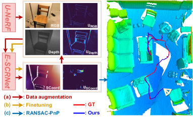
Figure 1: NeRF-enhanced SCR with uncertainty awareness. (a) We first train U-NeRF and E-SCRNet to perform informative data augmentation based on the uncertainties of rendered RGB-D images and predicted scene coordinates. (b) The E-SCRNet is finetuned on the augmented dataset considering pixelwise reliability. (c) Finally, the predicted 2D-3D correspondences with uncertainty are fed into PnP to estimate the camera poses.

II RELATED WORKS

Visual localization methods can be roughly categorized into three groups: Direct pose regression using Convolutional Neural Networks (CNN)  [5, 6, 7, 8, 9, 10]; Image retrieval with reference images tagged with known poses [11, 12, 13, 14]; Pose estimation from 2D-3D correspondences which are usually obtained by sparse feature matching [15, 16, 17, 18, 19, 20, 21, 22, 23, 24, 25, 26]. Scene coordinate regression adds another important branch to the third category. It obtains the correspondences by regressing dense 3D scene coordinates for the query image using random forests or neural networks, then calculates the final camera pose via RANSAC-PnP. Shotton et al. [20] propose to regress scene coordinates using a Random Forest, followed by several variants [27, 28, 29, 30, 31]. DSAC [32] and its follow-ups [33, 21] employ CNNs to predict the coordinate map and propose a differentiable approximation of RANSAC for end-to-end training. Li et al. [1] partition the scene into regions and hierarchically predict scene coordinates by adding several classification layers into a regression network. Huang et al. [2] partition the 3D surfaces into 3D patches and train a segmentation network to obtain correspondences between image pixels and patch centers. As a main bottleneck, these methods require large amounts of posed images to train their models.

NeRF [4] was introduced as a powerful technique for synthesizing novel views of complex scenes. Follow-up works try to add depth supervision to enhance quality [34, 35, 36], reduce data requirement [37, 38, 39], handle noisy or unknown camera pose [40, 41], speed up optimization or rendering [42, 43, 44, 45, 46] and extend to large-scale environments [47, 48, 49]. NeRF has been widely adopted for applications like navigation [50], manipulation [51], active 3D object reconstuction [52], data augmentation for learning object descriptors [53]. Sharing our spirit of adopting NeRF to synthesize novel views for visual localization, Zhang et al. iteratively refine camera poses based on feature matching between rendered and real images [54]. iNeRF [55] leverages NeRF’s differentiability and estimates camera poses in an analysis-by-synthesis manner. Chen et al. combine NeRF with pose regression by directly comparing the query and the rendered image [9]. The work is extended by adding feature matching with a random view synthesis strategy [10]. LENS [56] deploys NeRF-W [57] to synthesize views uniformly within the scene boundary to train a pose regression network. In this work, we propose to use NeRF to render data with high information gain for learning SCR.

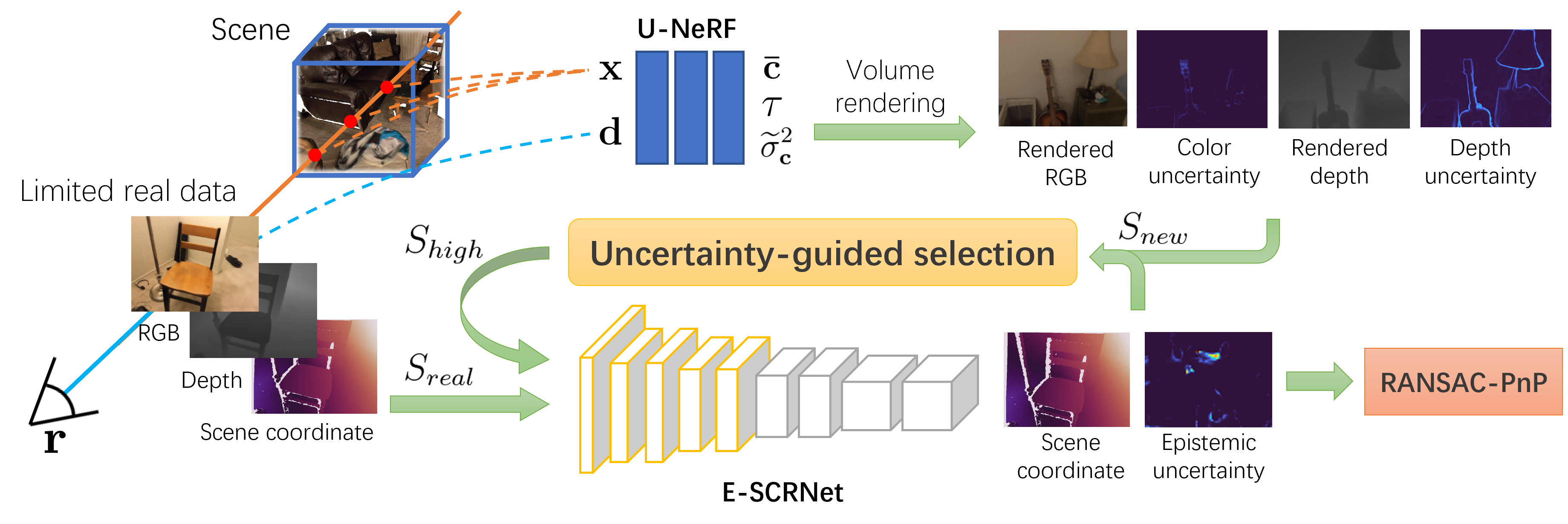
Figure 2: Overview. We first train an uncertainty-aware NeRF model and the evidential scene coordinate regression network (E-SCRNet) with the available data. We then render novel views with corresponding color and depth uncertainty maps. We apply an uncertainty-guided policy to select new views and gather them with the available data to finetune the E-SCRNet.

Uncertainty estimation for neural networks is relevant to assessing confidence, information gain and capturing outliers [58, 59, 60]. Bayesian neural networks [61, 62, 58] learn the posterior distribution of network weights and estimate it using variational inference, which can be approximated by Dropout or Deep Ensembles [63, 64, 65, 66]. However, they require expensive sampling during inference. Recently, evidential theory is incorporated into neural networks [67, 68], where training data add support to a learned higher-order evidential distribution. By learning the distribution hyperparameters, uncertainty can be estimated by a single forward pass, circumventing sampling during inference. For NeRF, NeRF-W [57] integrates uncertainty to attenuate transient scene elements. S-NeRF [69] encodes the posterior distribution over all the possible radiance fields and estimates uncertainty by sampling. CF-NeRF [70] follows a similar strategy and learns the radiance field distributions by coupling Latent Variable Modelling and Conditional Normalizing Flows. ActiveNeRF [71] models scene point radiance as Gaussian and uses uncertainty as a criterion for capturing new inputs.

III METHOD

SCR methods rely on large amounts of annotated training data that are hard to obtain in practice. To leverage synthetic data, NeRF can be used to render samples for arbitrary viewpoints using just a few posed images. However, the images rendered may be of low quality or highly redundant, which can lower the SCR network’s accuracy and efficiency. This motivates us to assess the quality and information gain of each view to make the best use of the synthetic data.

We first design U-NeRF and E-SCRNet. U-NeRF predicts color and depth uncertainties, reflecting the image quality, while E-SCRNet estimates the epistemic uncertainty of the predicted scene coordinates. Given a small set of real posed RGB-D images $S_{real}$, we train U-NeRF and an initial version of E-SCRNet. U-NeRF is used to generate a novel view dataset $S_{new}$ by synthesizing more views within the scene boundary (Sec. III-A). We feed $S_{new}$ to E-SCRNet to get the epistemic uncertainties, which reflect the information gain of each sample (Sec. III-B). We prune invalid views from $S_{new}$ based on U-NeRF’s uncertainties, then select views with high information gain $S_{high}$. The final augmented dataset, $S_{aug}=S_{real}\cup S_{high}$, is used to finetune E-SCRNet, increasing localization performance with higher data efficiency (Sec. III-C). Our overall pipeline is illustrated in Fig. 2.

III-A View synthesis with uncertainty estimation

Preliminaries on NeRF. NeRF models the scene as a continuous function using a multilayer perceptron (MLP). For a 3D position $\mathbf{x}$ and a viewing direction $\mathbf{d}$ that are transformed using positional encoding $\phi(\text{\textperiodcentered})$, the learned implicit function outputs a volume density $\tau$ and a view-dependent RGB color $\mathbf{c}$. To obtain the color of a pixel, consider the ray $\mathbf{r}(t)=\mathbf{o}+t\mathbf{d}$ emanating from the camera center $\mathbf{o}\in\mathbb{R}^{3}$ and traversing the range $[t_{n},t_{f}]$. Volume rendering computes light radiance by integrating the radiance along the ray. NeRF approximates it using hierarchical stratified sampling [72] by partitioning [$t_{n},t_{f}$] into $N$ bins and sampling uniformly in each bin. The expected color $\hat{\mathbf{C}}(\mathbf{r})$ can be approximated by

$$\hat{\mathbf{C}}(\mathbf{r})=\sum_{i=1}^{N}T_{i}\ (1-\exp{(-\tau_{i}\delta_{i})})\ \mathbf{c}_{i}=\sum_{i=1}^{N}w_{i}\mathbf{c}_{i},$$ (1)

where $T_{i}=\exp{(-\sum_{j=1}^{i-1}\tau_{j}\delta_{j})}$ and $\delta_{i}=t_{i+1}-t_{i}$. $\hat{\mathbf{C}}(\mathbf{r})$ therefore is a weighted sum of the color samples $\mathbf{c}_{i}$.

We aim to use NeRF to synthesize novel views for training the SCR network. However, the synthesized views may contain noises, blur, and other artifacts caused by varied imaging conditions of inputs. Training with such noisy samples can mislead the network from clean distribution and decrease its performance. To reason about the reliability of the rendered data, we formulate our scene representation with uncertainty estimation, named U-NeRF. One key observation is that the uncertainties of the rendered color and depth images should be modeled separately, as they present quite different distributions as shown in Fig. 4.

Color uncertainty. To estimate the color uncertainty, we assume the radiance value of a scene point to be Gaussian $\mathbf{c}_{i}\sim\mathcal{N}\left(\bar{\mathbf{c}}_{i},\bar{\sigma}_{\mathbf{c}_{i}}^{2}\right)$. The mean $\bar{\mathbf{c}}_{i}$ is the predicted radiance and the variance $\bar{\sigma}_{\mathbf{c}_{i}}^{2}$ captures the color uncertainty of a certain scene point. Employing Bayesian learning [58, 57, 71], we add an additional branch to predict $\bar{\sigma}_{\mathbf{c}_{i}}^{2}$ after injecting viewing directions: $(\tau,\bar{\mathbf{c}},\widetilde{\sigma}_{\mathbf{c}}^{2})=\text{MLP}\left(\phi\left(\mathbf{x},\mathbf{d}\right)\right)$. $\widetilde{\sigma}_{\mathbf{c}}^{2}$ is processed by a Softplus to obtain valid variance $\bar{\sigma}_{\mathbf{c}}^{2}$. When performing volume rendering as in Eq.1, the rendered pixel color can be viewed as a weighted sum of radiance colors $\mathbf{c}_{i}$. By assuming that the distributions of different sampled scene points on one ray are independent, and the distributions of sampled rays are independent, we can derive that the rendered pixel color follows a Gaussian distribution: $\hat{\mathbf{C}}\sim\mathcal{N}\left(\bar{\mathbf{C}},\bar{\sigma}_{\mathbf{C}}^{2}\right)\sim\mathcal{N}\left(\sum_{i=1}^{N}w_{i}\bar{\mathbf{c}}_{i},\sum_{i=1}^{N}w_{i}^{2}\bar{\sigma}_{\mathbf{c}_{i}}^{2}\right),$ where $w_{i}$ is defined in Eq.1, $N$ is the number of sampled points along the ray. $\bar{\mathbf{C}}$ and $\bar{\sigma}_{\mathbf{C}}^{2}$ are the mean and variance of the rendered pixel color (see Fig. 3). From a maximum likelihood perspective, we can optimize the model by minimizing the negative log-likelihood (NLL) loss for sampled rays $\mathbf{r}$ [57, 71]:

$$\mathcal{L}_{\mathrm{NLL}}=\sum_{\mathbf{r}\in R}\underbrace{\left(\frac{\|\mathbf{C}\left(\mathbf{r}\right)-\hat{\mathbf{C}}\left(\mathbf{r}\right)\|_{2}^{2}}{\hat{\sigma}_{\mathbf{C}}^{2}\left(\mathbf{r}\right)}+\log\hat{\sigma}_{\mathbf{C}}^{2}\left(\mathbf{r}\right)\right)}_{\mathcal{L}(\mathbf{r})}.$$ (2)

However, it leads to sub-optimal mean fits and premature convergence as badly-fit regions receive increasingly less weights. To address the ignorance of hard-to-fit regions, we add a variance-weighting term $\sigma_{\mathbf{C}}^{2\zeta}$ that acts as a factor on the gradient [73] as $\mathcal{L}_{\mathrm{color}}=\sum_{\mathbf{r}\in R}\left\lfloor\hat{\sigma}_{\mathbf{C}}^{2\zeta}\right\rfloor\mathcal{L}(\mathbf{r}),$ where $\left\lfloor\text{\textperiodcentered}\right\rfloor$ denotes the stop gradient operation which prevents the gradient from flowing through inside the parenthesis, making the variance-weighting term an adaptive learning rate. The parameter $\zeta$ interpolates between NLL ($\zeta=0$) and MSE ($\zeta=1$) while providing well-behaved uncertainty estimates. Note that NeRF-W [57] applies the volume rendering over $\sigma_{\mathbf{C}}$ instead of ${\sigma^{2}_{\mathbf{C}}}$, which is not theoretically grounded. Our approach is similar to ActiveNeRF [71], but we adopt a $\zeta$-NLL loss to cope with sub-optimal performance.

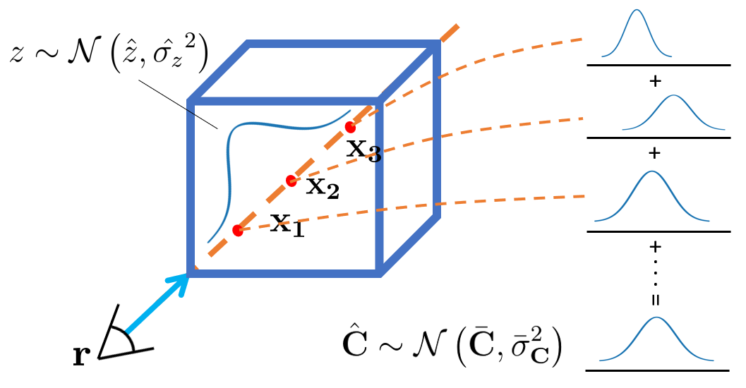
Figure 3: U-NeRF. If the distribution of a scene point’s radiance is Gaussian, the rendered pixel color is the weighted sum of Gaussians, thus still a Gaussian. We also assume the ray termination distribution $z$ to be Gaussian.

Depth uncertainty. Eq.1 can be slightly modified to obtain the expected depth $\hat{z}(\mathbf{r})$ of each ray and its variance $\hat{\sigma}_{z}(\mathbf{r})^{2}$: $\hat{z}(\mathbf{r})=\sum_{i=1}^{N}w_{i}t_{i},\quad\hat{\sigma}_{z}(\mathbf{r})^{2}=\sum_{i=1}^{N}w_{i}\left(t_{i}-\hat{z}(\mathbf{r})\right)^{2}.$ [36] demonstrates that adding depth supervision improves the reconstruction quality and leads to a change in the weight distribution from multimodal to unimodal. We assume the ray termination distribution to be Gaussian $z_{i}\sim\mathcal{N}\left(\hat{z}_{i},\hat{\sigma}_{z}(\mathbf{r})^{2}\right)$ and adopt a NLL on the output depth [34]:

$$\mathcal{L}_{\mathrm{depth}}=\sum_{\mathbf{r}\in R}\left(\frac{\left\|\hat{z}(\mathbf{r}))-z(\mathbf{r}))\right\|_{2}^{2}}{\hat{\sigma}_{z}(\mathbf{r})^{2}}+\log\hat{\sigma}_{z}(\mathbf{r})^{2}\right),$$ (3)

where $z(\mathbf{r})$ is the target depth. The variance $\hat{\sigma}_{z}(\mathbf{r})^{2}$ captures the uncertainty of the rendered depth (see Fig. 3).

Training U-NeRF. We optimize our scene representation with the objective function

$$\mathcal{L}_{\mathrm{overall}}=\mathcal{L}_{\mathrm{color}}+\lambda\mathcal{L}_{\mathrm{depth}}.$$ (4)

To reduce the training cost, we adopt a single MLP and optimize with depth-guided sampling [34].

III-B Evidential scene coordinate regression

For evaluating the potential contribution of each synthetic sample, we consider not only the rendering quality (reflected by uncertainties from U-NeRF) but also how informative the sample is for learning SCR. To this end, the epistemic uncertainty [59, 60, 74, 75] can be adopted to reflect the information gain the sample brings to the network. Compared to aleatoric uncertainty which represents the inherent randomness in data that cannot be explained away, epistemic uncertainty captures the uncertainty over network parameters and describes the confidence of the prediction [58]. Therefore, data samples with high epistemic uncertainty are associated with increased information gain. We propose to formulate scene coordinate regression from the perspective of evidential deep learning [67, 68], which enables fast sampling-free estimation of epistemic uncertainty. Since we aim to develop a general pipeline that can be applied to any SCR network, we take the simple regression-only baseline (SCRNet) from [1] as an example in this paper.

We assume the observed scene coordinates $q_{i}$ are drawn $\mathrm{i.i.d.}$ from an underlying Gaussian distribution with unknown mean $\mu_{q}$ and variance ${\sigma_{q}}^{2}$. To estimate the posterior distribution $p\left(\mu_{q},{\sigma_{q}}^{2}\mid q_{1},\ldots,q_{N}\right)$, we place priors over the likelihood variables with a Gaussian prior on ${\mu_{q}}\sim\mathcal{N}\left(\gamma,{\sigma_{q}}^{2}v^{-1}\right)$ and an Inverse-Gamma prior on ${\sigma_{q}}^{2}\sim\Gamma^{-1}(\alpha,\beta)$. Assuming that the posterior distribution can be factorized, we can approximate it with a Normal Inverse-Gamma (NIG) distribution [68] Sampling an instance from the NIG distribution yields a Gaussian distribution from which scene coordinates $q_{j}$ are drawn. Hence, the NIG distribution can be interpreted as the evidential distribution on top of the unknown likelihood distribution from which observations are drawn. By estimating the NIG hyperparameters $(\gamma,v,\alpha,\beta)$, we can compute the prediction $\mathbb{E}[\mu]=\gamma$ and epistemic uncertainty $\operatorname{Var}[\mu]=\beta/(v(\alpha-1))$. To train a network to output the correct scene coordinates and the hyperparameters of the corresponding NIG distribution, we modify the last layer of SCRNet to predict $(\gamma,v,\alpha,\beta)$, and maximize the model fit while minimizing evidence on errors [68]:

$$\mathcal{L}_{\mathrm{coord}}=\sum_{\mathbf{q}\in S}\left[\left(\alpha+1/2\right)\log\left(\left(q-\gamma\right)^{2}\nu+2\beta\left(1+\nu\right)\right)\right]$$ (5)

$$+\sum_{\mathbf{q}\in S}\left[\left(1/2\right)\log\left(\frac{\pi}{\nu}\right)-\alpha\log\left(2\beta\left(1+\nu\right)\right)\right]$$

$$+\sum_{\mathbf{q}\in S}\left[\log\left(\frac{\Gamma\left(\alpha\right)}{\Gamma\left(\alpha+1/2\right)}\right)+\left|q-\gamma\right|\cdot\left(2\nu+\alpha\right)\right].$$

In this way, the E-SCRNet regresses the scene coordinates for each pixel with corresponding uncertainty. We consider the epistemic uncertainty as a proxy for information gain and therefore a score in the following novel view selection policy. In addition, the uncertainty also reflects the confidence of the predicted 2D-3D correspondences. We can use it to filter out unreliable correspondences in RANSAC-PnP.

III-C Selection policy of novel views

With color and depth uncertainties from U-NeRF and epistemic uncertainty from E-SCRNet prepared, we are ready to select the most informative samples to boost the localization performance without introducing much computational cost. To generate the initial synthetic training data $S_{new}$, we use U-NeRF to render RGB-D images with uncertainty estimation from different viewpoints within the scene. Note that this view synthesizing process can be very fast with highly efficient NeRF rendering  [44, 46, 76]. We then propose the following two steps for data selection, i.e., rendering quality based pruning and information gain based selection.

Pruning based on rendering quality. Given the rendered color and depth uncertainties, we use the following criteria to remove inferior candidates: (1) views with rendered depth smaller than $z_{min}$ are too close to the scene structure and are considered invalid; (2) views with large depth uncertainty carry incorrect geometric information of the scene; (3) views with large color uncertainty contain noisy image texture that would confuse the SCRNet. This first round of pruning improves the overall quality of the rendered novel view set, but $S_{new}$ may still contain unnecessary redundancy. E.g., given a new view, if the SCRNet has already learned it well from $S_{real}$ and is very confident in its prediction, we know that the new view will bring little information gain. Therefore, another view selection step is performed.

Selection based on information gain. As mentioned in Sec. III-B, the epistemic uncertainty can be used as a proxy for information gain. We therefore propose a view selection policy guided by the scene coordinate epistemic uncertainty. For each of the rendered images in $S_{new}$, we apply the E-SCRNet pre-trained from $S_{real}$ to get the epistemic uncertainty map (together with the scene coordinate map). We aim to use the mean epistemic uncertainty as a novel view score. To remove the influence of rendered artifacts, the color and depth uncertainties provided by U-NeRF are used to filter out unreliable pixels. The images with the top-k scores are considered to provide high information gain and are selected to form the novel view set $S_{high}$.

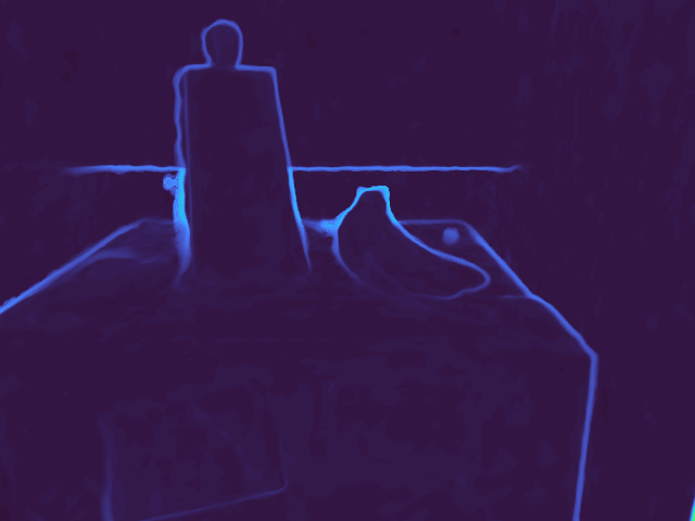
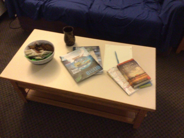
(a) GT color

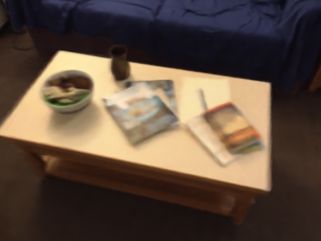
(b) Rendered color

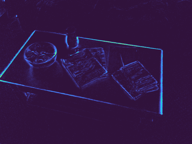
(c) Color error

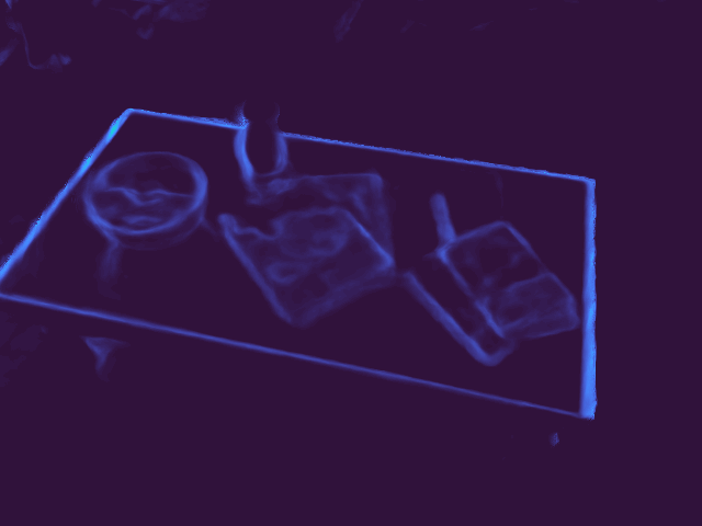
(d) Color uncertainty

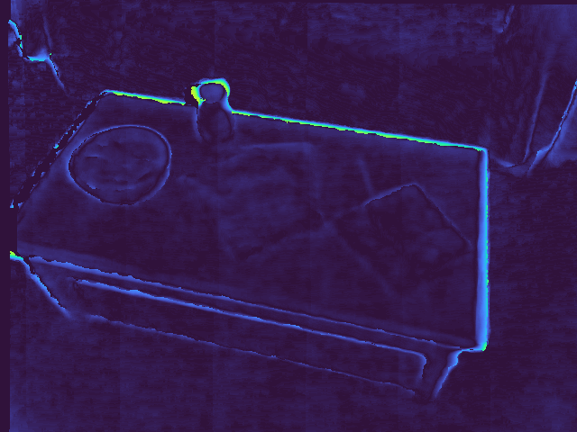
(e) Depth error

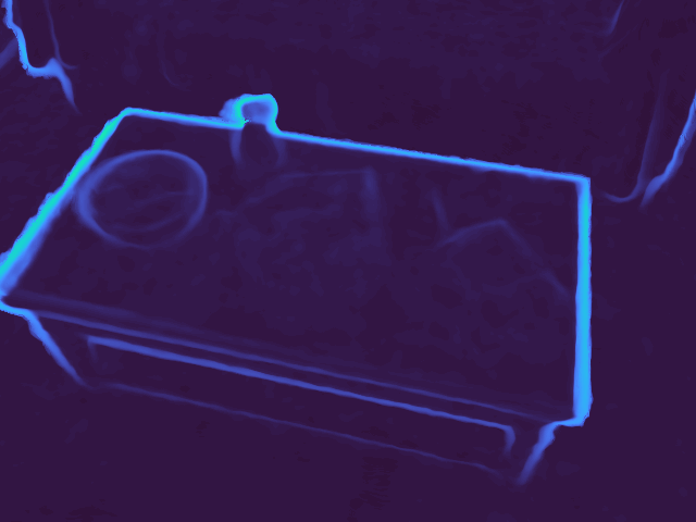
(f) Depth uncertainty

Figure 4: Qualitative results of U-NeRF uncertainty estimation.

Training with pixelwise uncertainty. In addition to bad sample pruning and view selection on image level, RGB-D uncertainties also indicate noises and artifacts on the pixel level. To alleviate the influences of these noisy rendered signals, we further adopt the pixel-wise RGB-D uncertainties into loss design. Firstly, pixels with uncertainties beyond the predefined thresholds are ignored in the loss. Secondly, they are used to weigh the remaining pixels. Since E-SCRNet is trained with color-depth pairs, we consider both uncertainties and formulate the weighting function as $\kappa=e^{-2({\sigma_{c}}^{2}+{\sigma_{z}}^{2})}$, then replace $\left(q-\gamma\right)$ with $\kappa\left(q-\gamma\right)$ in Eq.5. This weighting encourages E-SCRNet to memorize well-rendered regions better while paying less attention to uncertain regions.

IV Experiments

In this section, we conduct experiments to evaluate our pipeline. The results show that U-NeRF and E-SCRNet could provide meaningful uncertainties and our pipeline is able to improve camera pose estimation accuracy by a large margin.

TABLE I: Visual localization results on Replica. We report median and mean translation and rotation errors (cm,°). We also report the sum of the L1 distance between predicted scene coordinates and ground truth in $m$. The best results under the few views training are labeled in bold.

	SCRNet [1]			SCRNet-ID [77]			SRC [78]		Ours
	Median$\downarrow$	Mean$\downarrow$	Dist.	Median$\downarrow$	Mean$\downarrow$	Dist.$\downarrow$	Median$\downarrow$	Mean$\downarrow$	Median$\downarrow$	Mean$\downarrow$	Dist.$\downarrow$
room_0	2.05, 0.33	2.38, 0.36	0.27	2.33, 0.28	2.55, 0.32	0.24	2.78, 0.54	3.11, 0.64	1.53, 0.24	1.98, 0.27	0.22
room_1	1.84, 0.34	2.21, 0.42	0.21	1.83, 0.35	2.22, 0.42	0.20	1.92, 0.35	3.40, 0.74	1.96, 0.31	2.19, 0.38	0.17
room_2	1.31, 0.26	2.69, 0.65	0.37	1.78, 0.29	3.15, 0.69	0.39	2.97, 0.63	13.0, 3.44	1.34, 0.22	2.57, 0.55	0.30
office_0	1.69, 0.34	2.01, 0.45	0.17	1.79, 0.37	2.24, 0.51	0.19	1.45, 0.30	1.92, 0.43	1.61, 0.35	1.97, 0.44	0.15
office_1	2.10, 0.52	2.23, 0.63	0.34	1.65, 0.42	1.99, 0.55	0.26	2.07, 0.53	2.22, 0.59	1.54, 0.44	1.74, 0.53	0.22
office_2	2.21, 0.41	2.54, 0.49	0.29	2.07, 0.37	2.28, 0.41	0.27	2.53, 0.51	3.20, 0.64	1.69, 0.33	1.93, 0.37	0.25
office_3	2.13, 0.37	4.91, 0.94	0.44	1.79, 0.28	5.72, 1.14	0.40	3.44, 0.63	21.5, 7.95	2.40, 0.38	4.25, 0.86	0.36
office_4	2.25, 0.43	3.29, 1.03	0.40	2.42, 0.35	3.57, 0.95	0.38	4.84, 0.90	24.3, 6.18	1.69. 0.32	2.50, 0.86	0.35

IV-A Uncertainties of novel view synthesis

Fig. 4 qualitatively shows the error maps of the rendered RGB and depth images, as well as our predicted color and depth uncertainty maps. A comparison of the RGB and depth error maps reveals distinct distributions. E.g., in the example of the first row, large depth errors are mainly at structure borders, whereas large RGB errors mostly appear in highly textured areas. This observation verifies our idea of treating color and depth uncertainties separately. Further, a comparison of the error maps with the corresponding uncertainty maps ((c) to (d), (e) to (f)) shows a notable correlation, demonstrating the effectiveness of our estimated uncertainties. When using the rendered RGB-D data for other tasks, the uncertainty maps can provide valuable hints on the quality of the rendered data.

IV-B Camera pose estimation

Datasets. We evaluate our method on Replica [79], 12-Scenes [31], and 7-Scenes [20] datasets. Replica contains high-fidelity indoor scenes and is widely used by recent works of NeRFs and localization [80, 81, 82, 83]. We use the sequences recorded in [80], choosing the first sequence of each scene for training and the second for testing. 12-Scenes and 7-Scenes are both real-world indoor RGB-D datasets while the former has significantly larger environments.

Evaluation. Instead of using thousands of training images, we conduct the few views training experiments. We first sample a small fraction of the original data to build $S_{real}$. We create few-view datasets with a simple strategy: select one sequence from the training sequences of each scene and uniformly sample from it. For Replica, we uniformly sample 1/5 frames for the selected sequence. For 12-Scenes, given that the sequences have varying numbers of frames, we adhere to uniform sampling but aim to achieve comparable sizes ($\sim$200, which is about 5%$\sim$20% frames for each scene) for all scenes as for other datasets. For 7-Scenes, we choose one training sequence and uniformly sample 1/4 of its frames. The numbers of selected novel views $S_{high}$ for Replica, 12-Scenes, and 7-Scenes are 150, 120, and 100, respectively.

Baselines. We compare our method with SCRNet [1], SCRNet-ID [77], and SRC [78]. SCRNet is the regression-only baseline proposed by [1], based on which we built SCRNet-ID and E-SCRNet. SCRNet-ID utilizes the In-Distribution novel view selection policy proposed by [77] to obtain new synthetic views. SRC [78] is a recently proposed classification-based method for few-views scene-specific localization. We skip the experiments on 12-Scenes for SRC [78] since they leveraged the dataset to pre-train the classification network with Reptile [84] for model initialization.

TABLE II: Visual localization results on 7-Scenes and 12-Scenes. We report median translation and rotation errors (cm,°), and accuracy as the percentages of error <5cm, 5°. The best results are labeled in bold.

		SCRNet [1]		SCRNet-ID [77]		SRC [78]		Ours
		Acc.$\uparrow$	Med.$\downarrow$	Acc.$\uparrow$	Med.$\downarrow$	Acc.$\uparrow$	Med.$\downarrow$	Acc.$\uparrow$	Med.$\downarrow$
7S	chess	78.1	3.0, 1.1	76.1	3.1, 1.1	77.5	3.6, 1.1	80.2	2.7, 0.9
	fire	75.9	3.4, 1.4	74.1	3.3, 1.3	96.0	1.7, 0.6	85.3	2.6, 1.1
	heads	97.8	1.4, 0.9	96.0	1.4, 1.1	99.0	1.8, 1.2	97.0	1.3, 1.0
	office	59.0	4.3, 1.2	45.2	5.5, 1.5	42.3	5.6, 1.4	63.8	3.8, 1.1
	pumpkin	44.9	5.4, 1.3	43.0	5.6, 1.3	42.0	5.8, 1.5	47.3	5.2, 1.3
	redkitchen	31.6	7.1, 2.0	33.5	7.0, 2.1	25.6	6.9, 1.8	34.8	6.8, 1.9
	stairs	43.3	5.5, 1.5	50.9	4.9, 1.3	48.2	5.1, 1.4	61.3	4.5, 1.1
12S	kitchen-1	90.4	2.3, 1.3	87.1	2.6, 1.4	-	-	100	0.9, 0.5
	living-1	92.6	2.4, 0.8	91.4	2.0, 0.8	-	-	97.6	2.1, 0.6
	Bed	73.5	3.3, 1.5	82.3	2.0, 0.8	-	-	97.5	1.6, 0.7
	kitchen-2	88.5	2.1, 1.0	90.5	1.8, 0.9	-	-	97.1	1.2, 0.5
	living-2	61.8	4.2, 1.8	79.9	3.0, 1.2	-	-	95.1	2.0, 0.8
	luke	58.6	4.4, 1.4	73.3	3.7, 1.3	-	-	90.0	2.6, 1.0
	gates362	88.6	2.6, 0.8	87.6	2.1, 1.0	-	-	91.0	2.0, 0.8
	gates381	76.3	3.4, 1.4	82.8	2.9, 1.2	-	-	81.4	2.7, 1.2
	lounge	86.9	2.7, 0.9	78.9	3.4, 1.1	-	-	97.0	1.8, 0.6
	manolis	84.0	1.8, 1.0	85.3	2.6, 1.2	-	-	94.1	1.6, 0.7
	5a	65.9	3.6, 1.5	72.8	3.3, 1.2	-	-	80.3	2.5, 0.9
	5b	64.7	3.4, 1.2	66.7	3.8, 1.3	-	-	81.5	2.6, 0.8

Localization results. As shown in Table I and Table II, across all three datasets, our method achieves the best performance compared with all baselines. Our method significantly outperforms SCRNet, showing that incorporating synthesized novel views could effectively enhance performance by a large margin. A comparison between ours and SCRNet-ID indicates that our novel view selection policy can select more informative samples. Additionally, compared with SRC, it can be seen that our method makes better use of the available data and boosts the localization performance more.

IV-C Analysis

Novel views selection. We compare different selection policies of novel views on the Replica dataset. For each scene, we sort all the rendered views according to the epistemic uncertainty, then select the top 150 novel views with the highest score (High score policy), 150 novel views with the lowest score (Low score policy), and another 150 random novel views (Random policy) for comparison. We use these two novel view sets to finetune the same network, respectively. From Table III, we can see that the High score policy significantly enhances the localization performance while the Low score policy does not. It shows that the novel views with high scores provide high information gain to the model.

TABLE III: Views selection policy. We report median and mean pose errors in (cm,°), and the sum of the L1 distance between predicted scene coordinates and ground truth in $m$.

Scene	Policy	Median$\downarrow$	Mean$\downarrow$	Dist.$\downarrow$
room_0	Low score	2.07, 0.315	2.15, 0.322	0.232
	Random	1.84, 0.290	2.24, 0.318	0.227
	High score	1.53, 0.243	1.98, 0.270	0.219
room_1	Low score	2.17, 0.346	2.47, 0.418	0.191
	Random	2.32, 0.366	2.58, 0.417	0.186
	High score	1.96, 0.312	2.19, 0.389	0.173
room_2	Low score	1.64, 0.291	3.04, 0.671	0.387
	Random	1.86, 0.253	2.97, 0.635	0.314
	High score	1.34, 0.220	2.57, 0.557	0.302

Removing noisy regions with NeRF uncertainty. As shown in Fig. 5, the point cloud (left) generated from the raw RGB-D rendered by NeRF is noisy and might mislead the SCR model. With uncertainty estimation from U-NeRF, we can identify the low-quality regions. By applying the pruning and weighting scheme mentioned in Sec. III-C, we can eliminate unsatisfying parts from the raw output, resulting in a cleaner point cloud (compare middle vs. right). From Table IV, we can also observe that removing noisy parts improves the performance of E-SCRNet, demonstrating the importance of applying pruning and weighting using U-NeRF uncertainty.

TABLE IV: Effectiveness of evidential deep learning (EDL), adding novel views (NV), and U-NeRF uncertainty pruning. On scene luke of 12-Scenes.

Method	Acc.$\uparrow$	Median$\downarrow$	Mean$\downarrow$
SCRNet	58	4.39, 1.438	5.46, 1.930
$\Lsh$ + EDL	81	3.31, 1.289	3.73, 1.473
$\Lsh$ + EDL + NV	85	3.11, 1.115	3.36, 1.310
$\Lsh$ + EDL + NV + pruning	90	2.61, 1.020	2.89, 1.187

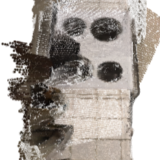
(a) Raw

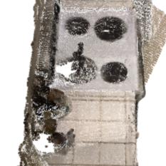
(b) Pruned

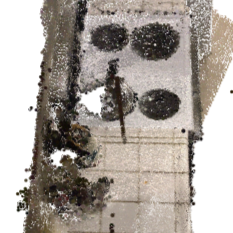
(c) Ground truth

Figure 5: Removing noisy regions using NeRF uncertainty.

Scene coordinate uncertainty. To evaluate the effectiveness of the predicted scene coordinate uncertainty, we train the SCRNet and E-SCRNet on the whole real training set with the same number of epochs, in chess of 7-Scenes. Then we compare their localization performance. In addition, for E-SCRNet, we sort the predicted 2D-3D correspondences with the estimated epistemic uncertainty. We then select the top 60% correspondences with the lowest uncertainty (denoted as confident) and the other correspondences (denoted as uncertain), and perform RANSAC-PnP to estimate poses, respectively. As shown in Table V, by comparing the 1 and the 2 row, E-SCRNet yields more accurate pose estimations than SCRNet when using all predicted correspondences. (It is also shown by comparing the 1 and the 2 row of Table IV.) E-SCRNet mitigates the influence of noisy samples and can better memorize the correct scene geometry during training, highlighting the importance of uncertainty estimation. Furthermore, the comparison between the 3 and the 4 row of Table V demonstrates that using correspondences with high confidence (low uncertainty) for camera pose optimization leads to more precise estimates. The correspondences with high uncertainty could noticeably downgrade the localization accuracy and increase pose errors, indicating the need to filter them out. It shows that the predicted uncertainty is meaningful. Lastly, if we compare the 2 and the 4 row of Table V, we can see that by using only the top 60% of confident correspondences we achieve the same localization performance as using all correspondences. More importantly, by using fewer correspondences we also largely speed up the running time for RANSAC, which improves the overall inference efficiency and benefits robotic applications.

TABLE V: Visual localization results on scene chess of 7-Scenes. We report median translation and rotation errors (cm,°), accuracy as the percentages of error <5cm, 5°, and the run time of RANSAC-PnP during pose estimation for one query image in milliseconds. The best results are labeled in bold.

	Acc.$\uparrow$	Med.$\downarrow$	Run time$\downarrow$
SCRNet [1], all	95.4	2.4, 0.73	30
E-SCRNet, all	97.4	2.0, 0.71	30
E-SCRNet, uncertain	93.6	2.4, 0.84	11
E-SCRNet, confident	97.4	2.0, 0.71	11

Comparing with all views results. We mainly focus on data efficiency so the few-view setting used was particularly challenging. As shown in Table VI, with 50% data our approach outperforms SCRNet trained on the full set and achieves even better performance when using all training data, indicating that our method requires only a small portion of training data but delivers comparable or even better performances than its counterpart trained on the full set.

TABLE VI: Comparing with all views results. (Acc. / Med. pose errors).

12Scenes	SCRNet [1] (All)	Ours (15%)	Ours (50%)	Ours (All)
luke	93.8 / 2.0, 0.9	90.0 / 2.6, 1.0	94.7 / 1.9, 0.7	95.8 / 1.4, 0.6
5b	93.3 / 1.9, 0.6	81.5 / 2.6, 0.8	95.8 / 1.7, 0.5	99.8 / 1.7, 0.5

Training time. To give an example, for manolis, training SCRNet with full set takes $\sim$2 days. For our pipeline, training U-NeRF and rendering images takes $\sim$6h, training E-SCRNet $\sim$5h, finetuning it $\sim$5h, together $\sim$16h. Such improvement was consistently observed on all used datasets. Moreover, recent advances in NeRF, which achieve speedy optimization and rendering, could further reduce the training time.

Applying to other SCR systems. We also apply our approach with DSAC* [21], improving its accuracy from 82.5% to 92.8%, and decreasing median translation and rotation errors from (3.3cm, 1.3°) to (2.0cm, 0.7°) on living-2 under the few views training setting, showing that our method can be applied to other SCR systems as a plug-in module, and enhance visual localization performances in a resource-efficient manner.

V Conclusion

We present a novel pipeline that leverages NeRF to generate RGB-D pairs for training SCR networks. By modeling the uncertainty in NeRF, we are able to filter out noisy regions and artifacts in the rendered data. By formulating SCR from the evidential deep learning perspective, we model the uncertainty over the predicted scene coordinates. We proposed an uncertainty-guided novel view selection policy that could select the samples that bring the most information gain and promote localization performance with the highest efficiency. Our method could be beneficial to many robotic applications.

References

- [1] X. Li, S. Wang, Y. Zhao, J. Verbeek, and J. Kannala, “Hierarchical scene coordinate classification and regression for visual localization,” in CVPR, 2020, pp. 11 983–11 992.
- [2] Z. Huang, H. Zhou, Y. Li, B. Yang, Y. Xu, X. Zhou, H. Bao, G. Zhang, and H. Li, “Vs-net: Voting with segmentation for visual localization,” in CVPR, 2021, pp. 6101–6111.
- [3] S. Tang, C. Tang, R. Huang, S. Zhu, and P. Tan, “Learning camera localization via dense scene matching,” in CVPR, 2021, pp. 1831–1841.
- [4] B. Mildenhall, P. P. Srinivasan, M. Tancik, J. T. Barron, R. Ramamoorthi, and R. Ng, “Nerf: Representing scenes as neural radiance fields for view synthesis,” CACM, vol. 65, no. 1, pp. 99–106, 2021.
- [5] A. Kendall and R. Cipolla, “Geometric loss functions for camera pose regression with deep learning,” in CVPR, 2017, pp. 5974–5983.
- [6] A. Kendall, M. Grimes, and R. Cipolla, “Posenet: A convolutional network for real-time 6-dof camera relocalization,” in ICCV, 2015, pp. 2938–2946.
- [7] T. Sattler, Q. Zhou, M. Pollefeys, and L. Leal-Taixe, “Understanding the limitations of cnn-based absolute camera pose regression,” in CVPR, 2019, pp. 3302–3312.
- [8] F. Walch, C. Hazirbas, L. Leal-Taixe, T. Sattler, S. Hilsenbeck, and D. Cremers, “Image-based localization using lstms for structured feature correlation,” in ICCV, 2017, pp. 627–637.
- [9] S. Chen, Z. Wang, and V. Prisacariu, “Direct-posenet: Absolute pose regression with photometric consistency,” in 3DV. IEEE, 2021, pp. 1175–1185.
- [10] S. Chen, X. Li, Z. Wang, and V. Prisacariu, “DFNet: Enhance absolute pose regression with direct feature matching,” in ECCV, 2022.
- [11] T. Sattler, T. Weyand, B. Leibe, and L. Kobbelt, “Image retrieval for image-based localization revisited.” in BMVC, vol. 1, no. 2, 2012, p. 4.
- [12] R. Arandjelovic and A. Zisserman, “All about vlad,” in CVPR, 2013, pp. 1578–1585.
- [13] A. Torii, R. Arandjelovic, J. Sivic, M. Okutomi, and T. Pajdla, “24/7 place recognition by view synthesis,” in CVPR, 2015, pp. 1808–1817.
- [14] R. Arandjelovic, P. Gronat, A. Torii, T. Pajdla, and J. Sivic, “Netvlad: Cnn architecture for weakly supervised place recognition,” in CVPR, 2016, pp. 5297–5307.
- [15] M. Dusmanu, I. Rocco, T. Pajdla, M. Pollefeys, J. Sivic, A. Torii, and T. Sattler, “D2-net: A trainable cnn for joint description and detection of local features,” in CVPR, 2019, pp. 8092–8101.
- [16] P.-E. Sarlin, C. Cadena, R. Siegwart, and M. Dymczyk, “From coarse to fine: Robust hierarchical localization at large scale,” in CVPR, 2019, pp. 12 716–12 725.
- [17] D. DeTone, T. Malisiewicz, and A. Rabinovich, “Superpoint: Self-supervised interest point detection and description,” in CVPR workshops, 2018, pp. 224–236.
- [18] L. Zhang and S. Rusinkiewicz, “Learning to detect features in texture images,” in CVPR, 2018, pp. 6325–6333.
- [19] H. Zhou, T. Sattler, and D. W. Jacobs, “Evaluating local features for day-night matching,” in ECCV. Springer, 2016, pp. 724–736.
- [20] J. Shotton, B. Glocker, C. Zach, S. Izadi, A. Criminisi, and A. Fitzgibbon, “Scene coordinate regression forests for camera relocalization in rgb-d images,” in CVPR, 2013, pp. 2930–2937.
- [21] E. Brachmann and C. Rother, “Visual camera re-localization from RGB and RGB-D images using DSAC,” TPAMI, 2021.
- [22] T. Sattler, B. Leibe, and L. Kobbelt, “Efficient & effective prioritized matching for large-scale image-based localization,” TPAMI, vol. 39, no. 9, pp. 1744–1756, 2016.
- [23] ——, “Improving image-based localization by active correspondence search,” in ECCV. Springer, 2012, pp. 752–765.
- [24] H. Taira, M. Okutomi, T. Sattler, M. Cimpoi, M. Pollefeys, J. Sivic, T. Pajdla, and A. Torii, “Inloc: Indoor visual localization with dense matching and view synthesis,” in CVPR, 2018, pp. 7199–7209.
- [25] P.-E. Sarlin, A. Unagar, M. Larsson, H. Germain, C. Toft, V. Larsson, M. Pollefeys, V. Lepetit, L. Hammarstrand, F. Kahl, et al., “Back to the feature: Learning robust camera localization from pixels to pose,” in CVPR, 2021, pp. 3247–3257.
- [26] P. Lindenberger, P.-E. Sarlin, V. Larsson, and M. Pollefeys, “Pixel-perfect structure-from-motion with featuremetric refinement,” in ICCV, 2021, pp. 5987–5997.
- [27] T. Cavallari, S. Golodetz, N. A. Lord, J. Valentin, L. Di Stefano, and P. H. Torr, “On-the-fly adaptation of regression forests for online camera relocalisation,” in CVPR, 2017, pp. 4457–4466.
- [28] L. Meng, J. Chen, F. Tung, J. J. Little, J. Valentin, and C. W. de Silva, “Backtracking regression forests for accurate camera relocalization,” in IROS. IEEE, 2017, pp. 6886–6893.
- [29] L. Meng, F. Tung, J. J. Little, J. Valentin, and C. W. de Silva, “Exploiting points and lines in regression forests for rgb-d camera relocalization,” in IROS. IEEE, 2018, pp. 6827–6834.
- [30] J. Valentin, M. Nießner, J. Shotton, A. Fitzgibbon, S. Izadi, and P. H. Torr, “Exploiting uncertainty in regression forests for accurate camera relocalization,” in CVPR, 2015, pp. 4400–4408.
- [31] J. Valentin, A. Dai, M. Nießner, P. Kohli, P. Torr, S. Izadi, and C. Keskin, “Learning to navigate the energy landscape,” in 3DV. IEEE, 2016, pp. 323–332.
- [32] E. Brachmann, A. Krull, S. Nowozin, J. Shotton, F. Michel, S. Gumhold, and C. Rother, “Dsac-differentiable ransac for camera localization,” in CVPR, 2017, pp. 6684–6692.
- [33] E. Brachmann and C. Rother, “Learning less is more-6d camera localization via 3d surface regression,” in CVPR, 2018, pp. 4654–4662.
- [34] B. Roessle, J. T. Barron, B. Mildenhall, P. P. Srinivasan, and M. Nießner, “Dense depth priors for neural radiance fields from sparse input views,” in CVPR, 2022, pp. 12 892–12 901.
- [35] Y. Wei, S. Liu, Y. Rao, W. Zhao, J. Lu, and J. Zhou, “Nerfingmvs: Guided optimization of neural radiance fields for indoor multi-view stereo,” in ICCV, 2021, pp. 5610–5619.
- [36] K. Deng, A. Liu, J.-Y. Zhu, and D. Ramanan, “Depth-supervised nerf: Fewer views and faster training for free,” in CVPR, 2022, pp. 12 882–12 891.
- [37] A. Chen, Z. Xu, F. Zhao, X. Zhang, F. Xiang, J. Yu, and H. Su, “Mvsnerf: Fast generalizable radiance field reconstruction from multi-view stereo,” in ICCV, 2021, pp. 14 124–14 133.
- [38] A. Yu, V. Ye, M. Tancik, and A. Kanazawa, “pixelnerf: Neural radiance fields from one or few images,” in CVPR, 2021, pp. 4578–4587.
- [39] D. Xu, Y. Jiang, P. Wang, Z. Fan, H. Shi, and Z. Wang, “Sinnerf: Training neural radiance fields on complex scenes from a single image,” arXiv preprint arXiv:2204.00928, 2022.
- [40] Z. Wang, S. Wu, W. Xie, M. Chen, and V. A. Prisacariu, “Nerf–: Neural radiance fields without known camera parameters,” arXiv preprint arXiv:2102.07064, 2021.
- [41] C.-H. Lin, W.-C. Ma, A. Torralba, and S. Lucey, “Barf: Bundle-adjusting neural radiance fields,” in ICCV, 2021, pp. 5741–5751.
- [42] A. Chen, Z. Xu, A. Geiger, J. Yu, and H. Su, “Tensorf: Tensorial radiance fields,” in ECCV, 2022.
- [43] C. Sun, M. Sun, and H.-T. Chen, “Direct voxel grid optimization: Super-fast convergence for radiance fields reconstruction,” in CVPR, 2022, pp. 5459–5469.
- [44] S. J. Garbin, M. Kowalski, M. Johnson, J. Shotton, and J. Valentin, “Fastnerf: High-fidelity neural rendering at 200fps,” in ICCV, 2021, pp. 14 346–14 355.
- [45] C. Reiser, S. Peng, Y. Liao, and A. Geiger, “Kilonerf: Speeding up neural radiance fields with thousands of tiny mlps,” in ICCV, 2021, pp. 14 335–14 345.
- [46] T. Müller, A. Evans, C. Schied, and A. Keller, “Instant neural graphics primitives with a multiresolution hash encoding,” ACM TOG, vol. 41, no. 4, pp. 102:1–102:15, July 2022. [Online]. Available: https://doi.org/10.1145/3528223.3530127
- [47] M. Tancik, V. Casser, X. Yan, S. Pradhan, B. Mildenhall, P. P. Srinivasan, J. T. Barron, and H. Kretzschmar, “Block-nerf: Scalable large scene neural view synthesis,” in CVPR, 2022, pp. 8248–8258.
- [48] K. Rematas, A. Liu, P. P. Srinivasan, J. T. Barron, A. Tagliasacchi, T. Funkhouser, and V. Ferrari, “Urban radiance fields,” in CVPR, 2022, pp. 12 932–12 942.
- [49] H. Turki, D. Ramanan, and M. Satyanarayanan, “Mega-nerf: Scalable construction of large-scale nerfs for virtual fly-throughs,” in CVPR, 2022, pp. 12 922–12 931.
- [50] M. Adamkiewicz, T. Chen, A. Caccavale, R. Gardner, P. Culbertson, J. Bohg, and M. Schwager, “Vision-only robot navigation in a neural radiance world,” IEEE RA-L, vol. 7, no. 2, pp. 4606–4613, 2022.
- [51] J. Ichnowski*, Y. Avigal*, J. Kerr, and K. Goldberg, “Dex-NeRF: Using a neural radiance field to grasp transparent objects,” in CoRL, 2020.
- [52] S. Lee, L. Chen, J. Wang, A. Liniger, S. Kumar, and F. Yu, “Uncertainty guided policy for active robotic 3d reconstruction using neural radiance fields,” IEEE RA-L, 2022.
- [53] L. Yen-Chen, P. Florence, J. T. Barron, T.-Y. Lin, A. Rodriguez, and P. Isola, “Nerf-supervision: Learning dense object descriptors from neural radiance fields,” arXiv preprint arXiv:2203.01913, 2022.
- [54] Z. Zhang, T. Sattler, and D. Scaramuzza, “Reference pose generation for long-term visual localization via learned features and view synthesis,” IJCV, vol. 129, no. 4, pp. 821–844, 2021.
- [55] L. Yen-Chen, P. Florence, J. T. Barron, A. Rodriguez, P. Isola, and T.-Y. Lin, “inerf: Inverting neural radiance fields for pose estimation,” in IROS. IEEE, 2021, pp. 1323–1330.
- [56] A. Moreau, N. Piasco, D. Tsishkou, B. Stanciulescu, and A. de La Fortelle, “Lens: Localization enhanced by nerf synthesis,” in CoRL. PMLR, 2022, pp. 1347–1356.
- [57] R. Martin-Brualla, N. Radwan, M. S. Sajjadi, J. T. Barron, A. Dosovitskiy, and D. Duckworth, “Nerf in the wild: Neural radiance fields for unconstrained photo collections,” in CVPR, 2021, pp. 7210–7219.
- [58] A. Kendall and Y. Gal, “What uncertainties do we need in bayesian deep learning for computer vision?” NeurIPS, vol. 30, 2017.
- [59] G. Georgakis, B. Bucher, K. Schmeckpeper, S. Singh, and K. Daniilidis, “Learning to map for active semantic goal navigation,” arXiv preprint arXiv:2106.15648, 2021.
- [60] G. Georgakis, B. Bucher, A. Arapin, K. Schmeckpeper, N. Matni, and K. Daniilidis, “Uncertainty-driven planner for exploration and navigation,” arXiv preprint arXiv:2202.11907, 2022.
- [61] D. J. MacKay, “Bayesian neural networks and density networks,” Nuclear Instruments and Methods in Physics Research Section A: Accelerators, Spectrometers, Detectors and Associated Equipment, vol. 354, no. 1, pp. 73–80, 1995.
- [62] I. Kononenko, “Bayesian neural networks,” Biological Cybernetics, vol. 61, no. 5, pp. 361–370, 1989.
- [63] Y. Gal and Z. Ghahramani, “Dropout as a bayesian approximation: Representing model uncertainty in deep learning,” in ICML. PMLR, 2016, pp. 1050–1059.
- [64] D. P. Kingma, T. Salimans, and M. Welling, “Variational dropout and the local reparameterization trick,” NeurIPS, vol. 28, 2015.
- [65] B. Lakshminarayanan, A. Pritzel, and C. Blundell, “Simple and scalable predictive uncertainty estimation using deep ensembles,” NeurIPS, vol. 30, 2017.
- [66] S. Jain, G. Liu, J. Mueller, and D. Gifford, “Maximizing overall diversity for improved uncertainty estimates in deep ensembles,” in AAAI, vol. 34, no. 04, 2020, pp. 4264–4271.
- [67] M. Sensoy, L. Kaplan, and M. Kandemir, “Evidential deep learning to quantify classification uncertainty,” NeurIPS, vol. 31, 2018.
- [68] A. Amini, W. Schwarting, A. Soleimany, and D. Rus, “Deep evidential regression,” NeurIPS, vol. 33, pp. 14 927–14 937, 2020.
- [69] J. Shen, A. Ruiz, A. Agudo, and F. Moreno-Noguer, “Stochastic neural radiance fields: Quantifying uncertainty in implicit 3d representations,” in 3DV. IEEE, 2021, pp. 972–981.
- [70] J. Shen, A. Agudo, F. Moreno-Noguer, and A. Ruiz, “Conditional-flow nerf: Accurate 3d modelling with reliable uncertainty quantification,” in ECCV, 2022.
- [71] X. Pan, Z. Lai, S. Song, and G. Huang, “Activenerf: Learning where to see with uncertainty estimation,” in ECCV, 2022.
- [72] N. Max, “Optical models for direct volume rendering,” IEEE TVCG, vol. 1, no. 2, pp. 99–108, 1995.
- [73] M. Seitzer, A. Tavakoli, D. Antic, and G. Martius, “On the pitfalls of heteroscedastic uncertainty estimation with probabilistic neural networks,” in ICLR, Apr. 2022. [Online]. Available: https://openreview.net/forum?id=aPOpXlnV1T
- [74] D. Pathak, D. Gandhi, and A. Gupta, “Self-supervised exploration via disagreement,” in ICML. PMLR, 2019, pp. 5062–5071.
- [75] H. S. Seung, M. Opper, and H. Sompolinsky, “Query by committee,” in COLT, 1992, pp. 287–294.
- [76] A. Yu, R. Li, M. Tancik, H. Li, R. Ng, and A. Kanazawa, “Plenoctrees for real-time rendering of neural radiance fields,” in ICCV, 2021, pp. 5752–5761.
- [77] T. Ng, A. Lopez-Rodriguez, V. Balntas, and K. Mikolajczyk, “Reassessing the limitations of cnn methods for camera pose regression,” 3DV, 2021.
- [78] S. Dong, S. Wang, Y. Zhuang, J. Kannala, M. Pollefeys, and B. Chen, “Visual localization via few-shot scene region classification,” arXiv preprint arXiv:2208.06933, 2022.
- [79] J. Straub, T. Whelan, L. Ma, Y. Chen, E. Wijmans, S. Green, J. J. Engel, R. Mur-Artal, C. Ren, S. Verma, et al., “The replica dataset: A digital replica of indoor spaces,” arXiv preprint arXiv:1906.05797, 2019.
- [80] S. Zhi, T. Laidlow, S. Leutenegger, and A. J. Davison, “In-place scene labelling and understanding with implicit scene representation,” in ICCV, 2021, pp. 15 838–15 847.
- [81] E. Sucar, S. Liu, J. Ortiz, and A. J. Davison, “imap: Implicit mapping and positioning in real-time,” in ICCV, 2021, pp. 6229–6238.
- [82] A. Rosinol, J. J. Leonard, and L. Carlone, “Nerf-slam: Real-time dense monocular slam with neural radiance fields,” arXiv preprint arXiv:2210.13641, 2022.
- [83] K. Yang, M. Firman, E. Brachmann, and C. Godard, “Camera pose estimation and localization with active audio sensing,” in ECCV. Springer, 2022, pp. 271–291.
- [84] A. Nichol, J. Achiam, and J. Schulman, “On first-order meta-learning algorithms,” arXiv preprint arXiv:1803.02999, 2018.