Extended Wigner’s friend paradoxes do not require nonlocal correlations

Abstract

Extended Wigner’s friend no-go theorems provide a modern lens for investigating the measurement problem, by making precise the challenges that arise when one attempts to model agents as dynamical quantum systems. Most such no-go theorems studied to date, such as the Frauchiger-Renner argument and the Local Friendliness argument, are explicitly constructed using quantum correlations that violate Bell inequalities. In this work, we show that such correlations are not necessary for having extended Wigner’s friend paradoxes, by constructing a no-go theorem utilizing a proof of the failure of noncontextuality. The argument hinges on a novel metaphysical assumption (which we term Commutation Irrelevance) that is a natural extension of a key assumption going into the Frauchiger and Renner’s no-go theorem.

In recent years, a number of extensions of the famous Wigner’s friend thought experiment [1] have been proposed [2, 3, 4, 5]. These extended Wigner’s friend (EWF) arguments aim to elucidate the difficulties that arise when one attempts to model an observing agent as a quantum system in their own right. Arguments of this sort were popularized in 2016 by Frauchiger and Renner [4], leading to debates on its assumptions, and on how different interpretations of quantum mechanics deal with such no-go theorems [6, 7, 8, 9, 2, 10, 11, 12, 13, 14, 15, 16, 17, 18, 19, 20, 21]. These discussions provide a fresh angle on the measurement problem in quantum theory [22, 23, 12, 24, 3]. A device-independent no-go theorem based on a similar EWF scenario has been developed, namely, the Local Friendliness no-go theorem [5, 25, 26, 27, 28]. A number of other no-go theorems have been introduced [29, 30, 17, 31, 32], although all of these are essentially variants of the Frauchiger-Renner or the Local Friendliness argument. For an introduction to Wigner’s friend and various extensions, see Ref. [2].

As has been recognized numerous times [19, 16, 33, 20, 8, 23, 2], the Frauchiger-Renner construction is built around the correlations arising in Hardy’s no-go theorem for Bell’s notion of local causality [34]. Indeed, the vast majority [5, 25, 4, 8, 23, 30, 29, 24, 35, 27, 3] of EWF paradoxes are built around such nonlocal  correlations— that is, spacelike-separated correlations that cannot be explained by any classical common cause explanation [37, 38, 39, 40, 41, 42].

In this work, we construct a paradox that is close in spirit to Frauchiger and Renner’s, but starting from contextual correlations for measurements on a single system—correlations which therefore do not involve Bell nonlocality in any way. To obtain such a paradox, it is necessary to extend one of the key assumptions made by Frauchiger and Renner slightly. However, we argue that the extended assumption has essentially the same motivations as Frauchiger and Renner’s assumption, and so our no-go theorem has the same metaphysical consequences, despite not making use of nonlocal correlations.

There are a few other works that attempt to construct EWF arguments on a single system [43, 44, 45, 46]. Refs. [45, 46] implement constructions similar to ours based on contextual correlations, but do not identify or motivate the critical assumption that (we will argue) is required. In addition, Ref. [45] applies the projection postulate to processes that are also treated unitarily in the argument, which undermines any apparent contradiction (see [2, Sec. III] and [22, 9, 47, 29]). Refs. [43, 44] are not focused on contextual correlations, but in any case rely on assumptions that can be viewed as problematic (see Ref. [2]). As such, we consider our argument to be the first complete EWF paradox constructed using sequential measurements on a single system.

Background Assumptions for EWF arguments.– A number of assumptions we consider here are common to most EWF arguments. One standard assumption is the Universality of Unitarity, dictating that all dynamics can be described unitarily, even those of macroscopic systems including observers. It follows that if an agent had sufficient (and extreme) technological capabilities, they could apply the inverse of the unitary describing a measurement to undo that measurement process. Such an agent is called a superobserver. We also make the standard assumption of Absoluteness of Observed Events [5, 48, 25, 26, 30] that the outcome obtained in a measurement performed by an observer is single and absolute—not relative to anyone or anything.

Another standard assumption for EWF no-go theorems is that the outcome for any single measurement (or outcomes for measurements done in parallel, if those outcomes are jointly observable) occurs at frequencies obeying the Born rule, in accordance with operational quantum theory. Here we only need the Possibilistic Born Rule, demanding that such outcomes never occur if the Born rule assigns probability 0 to them, and that otherwise, they sometimes occur.

We will make use of all the assumptions introduced above. Our no-go theorem also makes use of one novel assumption called Commutation Irrelevance, which will be introduced in due time.

The $5$-cycle noncontextuality scenario.–We first summarize the 5-cycle noncontextuality no-go theorem from Ref. [49, 50, 51], on which our EWF argument will be based. Recall that a Kochen-Specker noncontextual assignment [52] for a set of measurements is a deterministic assignment of outcomes to those measurements, such that the assignment for each measurement is independent of which other compatible measurements are performed jointly with it. (The requirement of determinism can in turn be motivated by the more general assumption of generalized noncontextuality introduced by Spekkens [53, 53], which is defined and used later in this work.)

Consider five binary-outcome measurements $\{M_{i}\}_{i\in\{1,2,...,5\}}$, where the pairs $\{(1,2),(2,3),(3,4),$ $(4,5),(5,1)\}$ are jointly measurable. Imagine that the system is prepared such that the observations for these five joint measurements satisfy

$$p(1,1|1,2)=0,$$ (1a)

$$p(0,0|2,3)=0,$$ (1b)

$$p(1,1|3,4)=0,$$ (1c)

$$p(0,0|4,5)=0,$$ (1d)

and

$$p(0,1|5,1)\neq 0.$$ (2)

Denoting the deterministic assignment of the outcome of measurement $M_{i}$ as $m_{i}$, Eq. (1) implies that

$$m_{1}=1\Rightarrow m_{2}=0\Rightarrow m_{3}=1\Rightarrow m_{4}=0\Rightarrow m_{5}=1.$$ (3)

Therefore, in every run of the experiment where the outcome of $M_{1}$ is $1$, the outcome of $M_{5}$ must be $0$. However, Eq. 2 tells us that in some runs of the protocol, the outcome of $M_{5}$ is $0$ and the outcome of $M_{1}$ is $1$. Thus, there is no Kochen-Specker noncontextual assignment for these runs.

The set of correlations in Eq. (1) and Eq. (2) has a quantum realization as follows. Consider a qutrit prepared in the state

$$|\eta\rangle:=\sqrt{\frac{1}{3}}(|0\rangle+|1\rangle+|2\rangle)\equiv\sqrt{\frac{1}{3}}(1,1,1)^{T},$$ (4)

where $T$ denotes transposition, and define measurements

$$M_{i}:=\{|v_{i}\rangle\langle v_{i}|,\mathbb{1}-|v_{i}\rangle\langle v_{i}|\},$$ (5)

with the states $|v_{i}\rangle$ defined as

$$\begin{split}&|v_{1}\rangle=\sqrt{\frac{1}{3}}(1,-1,1)^{T},\\ &|v_{2}\rangle=\sqrt{\frac{1}{2}}(1,1,0)^{T},\\ &|v_{3}\rangle=(0,0,1)^{T},\\ &|v_{4}\rangle=(1,0,0)^{T},\\ &|v_{5}\rangle=\sqrt{\frac{1}{2}}(0,1,1)^{T}.\end{split}$$ (6)

We take outcome $0$ of a given measurement to correspond to $\mathbb{1}-|v_{i}\rangle\langle v_{i}|$ and outcome $1$ to correspond to $|v_{i}\rangle\langle v_{i}|$. In this case, Eqs. (1a)-(1d) are satisfied while $p(0,1|5,1)=\big{|}\langle\eta|(\mathbb{1}-|v_{5}\rangle\langle v_{5}|)|v_{1}\rangle\big{|}^{2}=1/9\neq 0$, leading to Eq. (2). Hence, quantum theory is not consistent with noncontextuality.

An EWF scenario with measurements on a single system.—We now leverage these 5-cycle correlations to construct an EWF no-go theorem. The argument involves five friends (denoted $A_{1}$, …, $A_{5}$) who perform the five measurements $M_{i}$ defined in Eq. 5 sequentially on a single system $S$ prepared in the state $\ket{\eta}$ of Eq. 4, and a superobserver Wigner who undoes the first three of these measurements at particular times during the protocol.

By the assumption of Universality of Unitarity, each observer can be modeled as a quantum system—and indeed, as a qubit, since only two orthogonal (coarse-grained) states of the observer are relevant to the argument. If each measurement $M_{i}$ is performed in a sufficiently isolated environment, Universality of Unitarity further implies that it can be described by a unitary. In particular, if the measurements are performed in a manner that has minimal disturbance on system $S$, then each measurement $M_{i}$ can be modeled by a CNOT gate $U_{M_{i}}$ between the system $S$ and the agent $A_{i}$, namely,

$$U_{M_{i}}:={\rm CNOT}_{SA_{i}}$$ (7)

$$= \ket{v_{i}}\bra{v_{i}}_{\rm S}\otimes\mathbb{1}_{\rm A_{i}}+(\mathbb{1}-\ket{v_{i}}\bra{v_{i}})_{\rm S}\otimes(\ket{1}\bra{0}+\ket{0}\bra{1})_{\rm A_{i}}.$$

where $\ket{0}_{A_{i}}$ is the coarse-grained state of $A_{i}$ having observed outcome 0 and $\ket{1}_{A_{i}}$ is for having observed outcome 1. We follow a standard abuse of notation by letting $\ket{0}_{A_{i}}$ also denote the coarse-grained ‘ready’ state of the observer—that is, the initial state of each observer (prior to the measurement).

The superobserver Wigner is assumed to have perfect quantum control over the joint system of $A_{1}$, $A_{2}$, $A_{3}$, and $S$. In particular, we assume he has the (extreme) technological capabilities to implement the inverse of the unitary operations for the first three friends’ measurements.

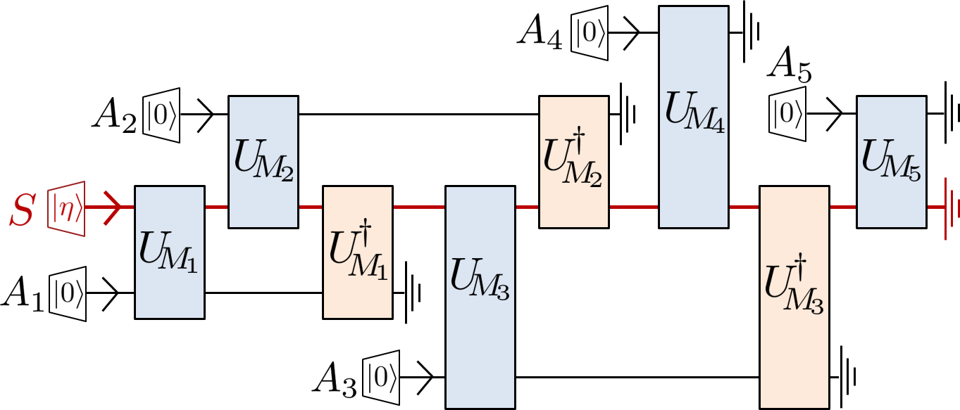
Figure 1: Five friends $A_{1},\dots,A_{5}$ perform the five measurements from a 5-cycle noncontextuality no-go theorem on a system $S$, while a superobserver Wigner undoes the first three of these measurements at particular times in between.

The exact sequence of operations is shown in the unitary circuit representation of the protocol in Fig. 1. Specifically, $M_{1}$ is the first measurement on $S$, followed by $M_{2}$, after which the superobserver undoes the first measurement by applying the unitary $U_{M_{1}}^{\dagger}$. Then $M_{3}$ is performed, followed by the undoing $U_{M_{2}}^{\dagger}$, followed by $M_{4}$, followed by the undoing $U_{M_{3}}^{\dagger}$, followed by $M_{5}$.

From Absoluteness of Observed Events, each agent $A_{i}$ observes an absolute outcome, denoted $a_{i}$, during their measurement $M_{i}$. We label the $\ket{v_{i}}\bra{v_{i}}$ outcome by $a_{i}=1$ and the other by $a_{i}=0$.

No-go theorem.—Measurements $M_{1}$ and $M_{2}$ are done immediately in sequence without any processes occurring in between, so the joint outcome $(a_{1},a_{2})$ can be directly observed (up until the time when $U_{M_{2}}^{\dagger}$ is performed). The Born rule predicts that

$$p(a_{1}=1,a_{2}=1)=0,$$ (8)

just as in Eq. 1a, the correlation for the $(1,2)$ pair of measurements in the 5-cycle noncontextuality scenario. Moreover, this Born rule prediction—and those that follow—can be made without appealing to the projection postulate, as we explain later.

Measurements $M_{2}$ and $M_{3}$ are not done immediately in sequence; rather, the unitary $U_{M_{1}}^{\dagger}$ is applied in between them. Nevertheless, the joint outcome $(a_{2},a_{3})$ is still directly observable (up until $U_{M_{2}}^{\dagger}$ is performed). The Born rule predicts that

$$p(a_{2}=0,a_{3}=0)=0,$$ (9)

just as in Eq. 1b, the correlation for the $(2,3)$ pair of measurements in the 5-cycle noncontextuality scenario. This is the case because the unitary $U_{M_{1}}^{\dagger}$ commutes with the $M_{3}$ measurement (as shown explicitly in Appendix V), and so it does not affect the Born rule prediction for $p(a_{2},a_{3})$.

Similarly, the Born rule predicts that

$$p(a_{3}=1,a_{4}=1)=0,$$ (10)

$$p(a_{4}=0,a_{5}=0)=0,$$ (11)

where both refer to joint outcomes that can be directly observed, and the only process happening between each pair of measurements is a unitary that commutes with those measurements (and so cannot affect their statistics). Eqs. 10 and 11 are analogous to Eqs. 1c and 1d, respectively, in the 5-cycle noncontextuality scenario.

However, the same argument cannot be applied to the joint outcome $(a_{1},a_{5})$, since it necessarily cannot be observed by any observer, even in principle. This is because the outcome $a_{1}$ is erased (by the unitary $U_{M_{1}}^{\dagger}$) prior to the outcome $a_{5}$ being generated. Consequently, even though the process $U:=U_{M_{3}}^{\dagger}U_{M_{4}}U_{M_{2}}^{\dagger}U_{M_{3}}U_{M_{1}}^{\dagger}U_{M_{2}}$, which is done between $M_{1}$ and $M_{5}$, commutes with $M_{5}$, the assertion that it does not affect the correlation between $M_{1}$ and $M_{5}$ is not guaranteed by the correctness of operational quantum theory (in particular, it does not follow from our assumption of Possibilistic Born Rule). Different interpretations of quantum theory may make different predictions for unobservable correlations, while still being consistent with operational quantum theory, as was highlighted already in, e.g., Ref. [2].

Therefore, to complete the argument, we require an assumption that the commutation relation $U_{M_{5}}UU_{M_{1}}=UU_{M_{5}}U_{M_{1}}$ implies $p_{U_{M_{5}}UU_{M_{1}}}(a_{1},a_{5})=p_{UU_{M_{5}}U_{M_{1}}}(a_{1},a_{5})$, where the former denotes the joint distribution when $U$ is performed between $M_{1}$ and $M_{5}$, and the latter denotes the joint distribution when $U$ is performed after $M_{5}$. Let us call this assumption Commutation Irrelevance. More generally, this assumption states that any unitary process performed between two measurements does not affect the correlations between their outcomes, provided that the unitary commutes with at least one of the two measurements—even if the outcomes of the two measurements are not jointly observable to any observer.

In the latter case, where $U$ is carried out after $M_{5}$, the correlation $p(a_{1},a_{5})$ is observable, and so is constrained by operational quantum theory to be $p_{UU_{M_{5}}U_{M_{1}}}(a_{1}=1,a_{5}=0)=0$. Consequently, assuming Commutation Irrelevance, the unobservable correlations for the actual experiment (where $U$ is done between $M_{1}$ and $M_{5}$) are constrained in the same way:

$$p(a_{1}=1,a_{5}=0)\neq 0.$$ (12)

This is analogous to Eq. 2 in the 5-cycle noncontextuality scenario.

Eqs. 8, 9, 10 and 11 imply that the actually observed outcomes must satisfy

$$a_{1}=1\Rightarrow a_{2}=0\Rightarrow a_{3}=1\Rightarrow a_{4}=0\Rightarrow a_{5}=1.$$ (13)

However, Eq. 12 tells us that the event $(a_{1}=1,a_{5}=0)$ occurs in some runs of the protocol.

Thus, we have a contradiction and consequently a no-go theorem against the conjunction of our assumptions: Universality of Unitarity, Absoluteness of Observed Events, Possibilistic Born Rule and Commutation Irrelevance.

In the Supplemental Material we extend these ideas to an infinite family of EWF paradoxes based on $n$-cycle proofs of the failure of Kochen-Specker noncontextuality for $n\geq 5$. We also introduce a unified description of possibilistic $n$-cycle contextuality models for both even and odd $n$.

How well motivated is Commutation Irrelevance?—No-go results are only as interesting as their underlying assumptions are compelling. Hence, it is necessary to question whether the assumption of Commutation Irrelevance is well-motivated. This is the key assumption beyond the standard assumptions common to EWF arguments, and plays a role analogous to the auxiliary assumptions of Timing Irrelevance or Local Agency in the Frauchiger-Renner and Local Friendliness arguments, respectively.

In fact, the assumption of Commutation Irrelevance is a minor extension of the assumption of Timing Irrelevance [2] required in the Frauchiger-Renner (and the Pusey-Masanes [31, 54]) arguments. Timing Irrelevance is the assumption that the correlations obtained in two quantum circuits whose only difference is the timing of the measurements must be identical (even if the difference in timings matters for the question of whether or not the correlations in question are in principle observable). Timing Irrelevance is a special case of Commutation Irrelevance, since the identity channel (representing the action of waiting) commutes with any operation.

Both Timing Irrelevance and Commutation Irrelevance can be motivated by the assumption that quantum theory is complete in the sense that there is no deeper theory or deeper set of facts (like hidden variables) that determine what measurement outcomes occur. This assumption is endorsed by researchers sympathetic to the Copenhagen school of thought. On the other hand, as argued in Ref. [2], for interpretations that violate Completeness, or researchers who are less certain that quantum theory is the deepest possible description of nature, Timing Irrelevance and Commutation Irrelevance may not be compelling assumptions.

One explicit example of an interpretation that violates Commutation Irrelevance is Bohmian mechanics. This follows from the fact that Bohmian mechanics violates even the weaker assumption of Timing Irrelevance, as discussed in Ref. [2]. One can also see Bohmian mechanics’s violation of Commutation Irrelevance in the scenario discussed here by noticing that Bohmian mechanics reproduces quantum predictions for observable correlations. For our scenario (where $U$ is done between $M_{1}$ and $M_{5}$), Bohmian mechanics reproduces the observable predictions that $a_{1}=1\Rightarrow a_{2}=0\Rightarrow a_{3}=1\Rightarrow a_{4}=0\Rightarrow a_{5}=1$. Hence, $p_{U_{M_{5}}UU_{M_{1}}}(a_{1}=1,a_{5}=0)=0$ holds. However, for the case where $U$ is done after $M_{5}$, so that the outcomes of $M_{1}$ and $M_{5}$ can be jointly observed, Bohmian mechanics reproduces the quantum prediction for this correlation, namely, that $p_{UU_{M_{5}}U_{M_{1}}}(a_{1}=1,a_{5}=0)\neq 0$. So in Bohmian mechanics, $p_{U_{M_{5}}UU_{M_{1}}}(a_{1}=1,a_{5}=0)\neq p_{UU_{M_{5}}U_{M_{1}}}(a_{1}=1,a_{5}=0)$.

Why one can (but should not) justify Commutation Irrelevance using noncontextuality.—A natural temptation is to justify Commutation Irrelevance by appealing to generalized noncontextuality [53]. Specialized to quantum theory, generalized noncontextuality is the assumption that two operational processes that have the same quantum representation are modeled as identical stochastic processes in an ontological model. This assumption has been given much motivation in the literature [53, 55, 56], particularly by appealing to a version of Leibniz’s principle [57] of the identity of indiscernible.

To do so, consider again the process $U=U_{M_{3}}^{\dagger}U_{M_{4}}U_{M_{2}}^{\dagger}U_{M_{3}}U_{M_{1}}^{\dagger}U_{M_{2}}$ that is done between $M_{1}$ and $M_{5}$, and recall that $U$ commutes with $M_{5}$. Consequently, the measurement $M_{5}$ is operationally equivalent to the effective measurement obtained by first applying $U$ to one’s system and then measuring $M_{5}$ (where in both cases we are considering $M_{5}$ as a terminal measurement). In a noncontextual model, then, the response functions associated with these two measurements must be identical. As such, the correlations between $M_{1}$ and $M_{5}$ cannot depend on whether or not $U$ is done in between them.

However, if one includes noncontextuality among one’s assumptions in an EWF no-go theorem, then one’s theorem will have no new foundational implications—rather, it will just become a worse proof of the failure of generalized noncontextuality. This is because in addition to the usual assumptions required in noncontextuality no-go theorems (chiefly, the assumption of tomographic completeness [53, 58]), one also requires the baggage of superobservers.

As an aside, if one were content to assume noncontextuality, one could construct a no-go theorem that is considerably simpler—one which does not appeal to any commutation arguments, and where the only operational equivalences required are of the form $UU^{\dagger}=\mathbb{1}$. Namely, one could merely consider an experiment wherein all five measurements ($M_{1}$ through $M_{5}$) are done in sequence, but with each measurement reversed by a superobserver in between. Then, because $M_{i}$ followed by $M_{i}^{\dagger}$ is operationally equivalent to the identity channel, generalized noncontextuality implies that the ontological representation of $M_{i}$ followed by $M_{i}^{\dagger}$ is given by the identity channel on the ontic state space. Consequently, all five measurements are performed on exactly the same ontic state, and so the fact that there is no consistent deterministic value assignment to these five measurements gives a contradiction.

Why our argument does not appeal to the projection postulate.—The most obvious textbook quantum prescription for computing the predictions in Eqs. 8, 9, 10, 11 and 12 makes use of the projection postulate, since each such prediction involves two measurements implemented in sequence. However, we emphatically do not wish to appeal to the projection postulate. As argued in Ref. [2, Sec. III] and [22, 9, 47, 29], one should expect inconsistencies in any argument that requires one to treat a given process both unitarily and via the projection postulate, and so EWF arguments are only nontrivial if they ensure that for each given process in the argument, one gives either a unitary description or a projection postulate description.

Consider for example the correlation for $(a_{1},a_{2})$. We do not wish to compute this correlation via $p(a_{1},a_{2})=\Tr[\Pi_{a_{2}}(\Pi_{a_{1}}\rho\Pi_{a_{1}})]$ (where $\Pi_{a_{i}}$ denotes the respective projector) as this equation uses the projection postulate. Because measurement $M_{1}$ and $M_{2}$ are compatible, operational quantum theory gives a prescription for computing probabilities for their joint outcomes that does not involve the projection postulate. In particular, the probability distribution $p(a_{1},a_{2})$ for $M_{1}$ and $M_{2}$ measured in sequence (provided $M_{1}$ is measured in a minimally disturbing manner) can be inferred from the probabilities assigned to a single measurement in the eigenbasis which simultaneously diagonalizes $M_{1}$ and $M_{2}$; namely, the measurement $M=\{\ket{v_{1}}\bra{v_{1}},\ket{v_{2}}\bra{v_{2}},\mathbb{1}-\ket{v_{1}}\bra{v_{1}}-\ket{v_{2}}\bra{v_{2}}\}$. If we imagine a hypothetical experiment where Alice performs this three-outcome measurement, then one can compute the probabilities $p(a_{1},a_{2})$ for the actually performed measurements $M_{1}$ and $M_{2}$ from it.

To be sure, the actual experiment does not involve the implementation of this joint measurement. We are only claiming that the statistics for the joint outcome $(a_{1},a_{2})$ can be computed by considering this hypothetical experiment, and that this computation does not require the projection postulate.

An analogous argument can be made for the correlation $p(a_{2},a_{3})$, but one must additionally note that the undoing operation $U_{M_{1}^{\dagger}}$ that is done between $M_{2}$ and $M_{3}$ cannot affect their outcome statistics, since it commutes with them, as noted earlier. A similar argument applies to $(a_{3},a_{4})$ and $(a_{4},a_{5})$.

For Eq. (12), the correlation $p(a_{1},a_{5})$ is unobservable to anyone, and so it is not constrained by operational quantum theory alone. But given Commutation Irrelevance, this unobservable correlation is equal to the observable correlation $p_{U_{M_{1}}U_{M_{5}}U}(a_{1},a_{5})$ in an experiment where $U$ is carried out after $M_{5}$ rather than before it. Because the latter correlation is observable, it is constrained by the predictions of operational quantum theory, and so we can again appeal to a measurement that jointly simulates $M_{1}$ and $M_{5}$ to compute the Eq. (12) without appealing to the projection postulate.

This establishes how one can obtain Eqs. (8)-(12) without using the projection postulate.

Future directions.—Exactly like the Frauchiger-Renner argument, our EWF no-go theorem is not an experimentally testable argument since not all correlations needed in the argument are observable. Nevertheless, it is a no-go theorem for quantum theory. It remains to be seen whether a device-independent argument of this sort can be constructed. Our results also open the possibility of new EWF scenarios constructed around other Kochen-Specker contextuality proofs. Our work also calls for further investigation into the importance of different forms of nonclassicality in EWF paradoxes.

Acknowledgements.—We thank Ernesto Galvão, Rui Soares Barbosa, Leonardo Santos, Sidiney Montanhano, Vilasini Venkatesh, Nuriya Nurgalieva, Howard Wiseman, and Matthew Leifer for their comments and useful discussions. LW also thanks Matt Pusey and Stefan Weigert for many discussions on the Frauchiger-Renner paradox.

RW acknowledges support from FCT – Fundação para a Ciência e a Tecnologia (Portugal) through PhD Grant SFRH/BD/151199/2021. LW acknowledges support from the United Kingdom Engineering and Physical Sciences Research Council (EPSRC) DTP Studentship (grant number EP/W524657/1). LW also thanks the International Iberian Nanotechnology Laboratory – INL in Braga, Portugal and the Quantum and Linear-Optical Computation (QLOC) group for the kind hospitality. DS was supported by the Foundation for Polish Science (IRAP project, ICTQT, contract no. MAB/2018/5, co-financed by EU within Smart Growth Operational Programme). YY was supported by Perimeter Institute for Theoretical Physics. Research at Perimeter Institute is supported in part by the Government of Canada through the Department of Innovation, Science and Economic Development and by the Province of Ontario through the Ministry of Colleges and Universities. YY was also supported by the Natural Sciences and Engineering Research Council of Canada (Grant No. RGPIN-2017-04383).

Supplemental Material for: Extended Wigner’s friend paradoxes do not require nonlocal correlations

In this supplemental material, we introduce a unified presentation of $n$-cycle arguments for $n$ even and odd, we prove the commutation relations mentioned in the main text, and most importantly, we show that similar extended Wigner’s friend (EWF) paradoxes to those constructed in the main text exist, if instead of considering $A_{1},\dots,A_{5}$ once considers $A_{,}\dots,A_{n}$, for any $n\geq 5$.

I Kochen-Specker contextuality

I.1 General framework

Kochen-Specker contextuality is a specific property of probabilistic data defined over measurement scenarios. We define a measurement scenario, also known as a compatibility scenario, as any triplet $(X,\mathcal{M},O)$ of a set of ideal measurements $X$, a set of maximal contexts $C\in\mathcal{M}$ , with each $C$ corresponding to a set of compatible measurements (i.e., jointly measurable elements from $X$), and a set of labels for possible outcomes $O$ that each measurement can return. We will consider only finite sets of outcomes $O$, but scenarios with infinite outcomes can be properly studied [60].

In the compatibility hypergraph approach [61, Chapter 2] (see also Ref. [62]) we encode the information of maximal contexts $C\in\mathcal{M}$ of a given scenario $(X,\mathcal{M},O)$ in a hypergraph where each node represents an element of $X$ and hyperedges correspond to elements from $\mathcal{M}$, i.e., maximal contexts. In such a graph, hence, edges connect compatible measurements. In Fig. 2 we depict the most studied and simplest non-trivial family of compatibility hypergraphs, known as $n$-cycle compatibility scenarios. Since in this case all hyperedges have only two elements, representing binary contexts, the hypergraphs reduce to graphs. Each such graph defines an infinite family of possible measurement scenarios, depending on the outcome set $O$ of the corresponding measurements.

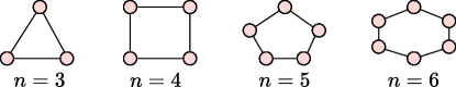
Figure 2: $n$-cycle compatibility hypergraphs. Cycle graphs $C_{n}$ for $n=3,4,5,6$. Each graph defines a compatibility structure that can be associated with measurement scenarios. Graph $C_{4}$ depicts the compatibility structure of the bipartite Bell scenarios leading to the Clauser-Horne-Shimony-Holt (CHSH) inequality [63]. Graph $C_{5}$ depicts the compatibility structure leading to the Klyachko-Can-Binicioğlu-Shumovsky (KCBS) inequality [50].

A behavior over a given finite measurement scenario is defined as a set of probability distributions over the maximal contexts,

$$\left\{p(\cdot|C):O^{C}\to[0,1]\bigr{|}\sum_{s\in O^{C}}p(s|C)=1,C\in\mathcal{M}\right\}.$$ (14)

Each $s\in O^{C}$ is simply a tuple of possible outcomes resulting from jointly measuring a given system with all the ideal measurements in $C\in\mathcal{M}$. A behavior is said to be non-disturbing whenever the marginals over intersections of contexts are equal, i.e., for all $C,C^{\prime}\in\mathcal{M}$ such that $C\cap C^{\prime}\neq\emptyset$ then $\sum_{s\in O^{C};s|_{C\cap C^{\prime}}=t}p(s|C)=\sum_{s^{\prime}\in O^{C^{\prime}};s^{\prime}|_{C\cap C^{\prime}}=t}p(s^{\prime}|C^{\prime})$ for all $t\in O^{C\cap C^{\prime}}$. The condition above becomes mathematically equivalent to the non-signalling condition in case the compatibility structure of the scenario is the one from a Bell scenario. If there exists a single probability distribution $g$ over $X$ that correctly reproduces the behavior by marginals over contexts, i.e.,

$$p(s|C)=\sum_{t\in O^{X};t|_{C}=s}g(t)$$ (15)

for all $C\in\mathcal{M}$ and $s\in O^{C}$, $g$ is said to be a global distribution and the behavior $\{p(s|C)\}_{s\in O^{C},C\in\mathcal{M}}$ is said to be noncontextual. Hence, a behavior is said to be contextual whenever such a global distribution $g$ cannot exist.

The conditions above are theory-independent, i.e. they do not assume that a given behavior can be reached using quantum theory. We say that a behavior $\{p(s|C)\}$ defined with respect to a scenario $(X,\mathcal{M},O)$ has a quantum realization whenever there exists some Hilbert space $\mathcal{H}$ for which each measurement in $M\in X$ corresponds to a projective measurement $\{P^{M}_{i}\}_{i=1}^{|O|}$, and such that there exists some density matrix $\rho$, i.e. a prepared state of some system, such that, letting $s=(o_{1},\dots,o_{n})$ and $C=\{M_{1},\dots,M_{n}\}$ we have $p(s|C)=\text{Tr}(\prod_{i=1}^{n}P_{o_{i}}^{M_{i}}\rho)$.

Let $\{p(s|C)\}$ be any behavior for a given scenario $(X,\mathcal{M},O)$. We define the possibilistic collapse of this behavior as the set $\{\overline{p}(s|C)\}$ defined by the functions $\overline{p}(-|C):O^{C}\to\{0,1\}$ for which

$$\overline{p}(s|C):=\left\{\begin{matrix}1&\text{if }p(s|C)>0\\ 0&\text{if }p(s|C)=0\end{matrix}\right..$$ (16)

We call $\{\overline{p}(s|C)\}$ a possibilistic behavior [64]. We say that a behavior $\{p(s|C)\}$ from a scenario $(X,\mathcal{M},O)$ is logically contextual whenever there exists some $s\in O^{C}$ and some $C\in\mathcal{M}$ such that (i) $p(s|C)>0$, (ii) for $t\in\{u\in O^{X}:u|_{C}=s\}$ there exists some $C^{\prime}\in\mathcal{M}$ such that $p(t|_{C^{\prime}}|C^{\prime})=0$. In words, if there exists some possible joint outcome $s\in O^{C}$ for which all global assignments $t$ consistent with $s$ over $C$, i.e. satisfying $t|_{C}=s$, are impossible when restricted to some other context $C^{\prime}$. Logically contextual behaviors lead to the so-called possibilistic paradoxes as merely the possibility of outcome results lead to paradoxical reasoning when assuming the existence of pre-determined values for all measurements simultaneously. Refs. [51, 49] constructed possibilistic paradoxes for any $n$-cycle scenario where all measurements are dichotomic.

I.2 An $n$-cycle logical contextual model

We present now the generalisation of the above 5-cycle logical contextual model to $n$-cycle logical contextuality scenarios, as shown in Refs. [49, 51]. We provide a similar theory-independent operational description of an experiment consisting of $n$ boxes, which can be either full or empty, as before. Checking whether a box is empty or full is again considered as a measurement. The contexts, in this case the boxes that can be opened together, are the measurements of box $m\bmod n$ and $(m+1)\bmod n$, with the same compatibility structure from Fig. 2. The logically contextual $n$-cycle behaviours for $n$ odd or even are usually discussed in slightly different terms, as we review in Section II. In Section III we show that how to transform the arguments in literature for odd and even $n$ into one single form, that is the one we present next.

The logically contextual behaviour for $n$-cycle scenarios, for any $n\geq 4$, is given by

$$p(0,1|i,i+1)=0\text{ for $1\leq i<n$},$$ (17)

and

$$p(0,1|1,n)>0.$$ (18)

These behaviours can be realized using quantum theory, from the behaviours of Ref. [51], which have a quantum realisation as described in Ref. [51, Eqs. (49)-(55)], once some relabeling of outcomes is introduced, as we describe in detail in Section III. There, we also describe how the 5-cycle behaviour as described above in can be put into this form, when relabeling measurement outcomes.

II Logically contextual $n$-cycle behaviour for odd and even $n$

In this appendix we start by presenting the logically contextual $n$-cycle behaviours from Ref. [51]. As we will see, the quantum realizations for behaviours constructed for $n$ odd or even are slightly different. We will then show in Appendix III that a unified description for these specific behaviours exists, relaxing such apparent asymmetry between behaviors in even and odd scenarios. This unified description is the one we have used in the main text.

An odd $n$-cycle logically contextual model.– We start presenting $n$-cycle logically contextual behaviors, with $n\geq 5$ an odd natural number. The system is prepared such that

$$p(1,1|1,2)=0,$$

$$p(0,0|2,3)=0,$$

$$\hskip 28.45274pt\vdots$$ (19)

$$p(1,1|n-2,n-1)=0,$$

$$p(0,0|n-1,n)=0,$$

and

$$p(0,1|n,1)>0.$$ (20)

If one assumes that the result of finding a box empty or full is predetermined and independent of which boxes are opened (i.e. noncontextuality), then the first equations imply that

$$p(0,1|n,1)=0,$$ (21)

in contradiction with Eq. (20). This model is thus logically contextual, with respect to the definitions provided in the main text, and has a quantum representation for any odd $n\geq 5$ [49, 51].

An even $n$-cycle logically contextual model.–We now construct a logically contextual $n$-cycle behavior, with $n\geq 4$ being an even natural number, following closely Ref. [51]. The behavior is defined such that

$$p(1,0|1,2)=0,$$

$$\hskip 28.45274pt\vdots$$

$$p\left(1,0\Bigr{|}\frac{n}{2}-1,\frac{n}{2}\right)=0,$$

$$p\left(1,1\Bigr{|}\frac{n}{2},\frac{n}{2}+1\right)=0,$$ (22)

$$p\left(0,1\Bigr{|}\frac{n}{2}+1,\frac{n}{2}+2\right)=0,$$

$$\hskip 28.45274pt\vdots$$

$$p(0,1|n-1,n)=0,$$

and

$$p(1,1|n,1)>0.$$ (23)

If one assumes that the result of finding a box empty or full is predetermined and independent of which boxes are opened (i.e. noncontextuality), then Eqs. (22) imply that

$$p(1,1|n,1)=0,$$ (24)

in contradiction with Eq. (23). This behavior is logically contextual and has a quantum realization, for any even $n\geq 4$ [51]. To do so, one can prepare a two-qubit system that satisfies Eqs. (22) and Eq. (23) when choosing appropriate projective measurements [51].

III Turning an odd $n$-cycle paradox into an even $n$-cycle paradox and vice versa

In this appendix we show that by relabeling the outcomes $0\leftrightarrow 1$ of measurements for $n$-cycle scenarios, we can transform the argument for odd $n$-cycle logical contextuality, as described in Section II, in the same form as the argument for even $n$-cycle logical contextuality from Section II, and vice versa. In this way, we can present the logically contextual behaviours for odd and even $n$-cycles as presented in Section II of [51], which are quantum realisable, in a uniform way.

III.1 Relabeling outcomes in odd $n$-cycle logical contextuality

Let $n$ be odd, and let us start from the odd $n$-cycle logical contextuality of Eqs. (19), (20):

$$p(1,1|1,2)=0,$$

$$p(0,0|2,3)=0,$$

$$\hskip 28.45274pt\vdots$$ (25)

$$p(1,1|n-2,n-1)=0,$$

$$p(0,0|n-1,n)=0,$$

and

$$p(0,1|n,1)>0.$$ (26)

Here, as before, $p(\cdot,\cdot|i,j)$ denotes the empirical probability distribution corresponding to the context where measurement $i$ and $j$ are jointly measured.

Let us consider the following relabeling of measurements (recall that $n$ is odd):

$$\begin{split}M_{1}&:\text{relabel},\\ M_{2}&:\text{keep},\\ M_{3}&:\text{relabel},\\ M_{4}&:\text{keep},\\ \vdots\\ M_{n}&:\text{relabel},\end{split}$$ (27)

i.e., relabeling the outcomes of all odd measurements. By ‘relabel’ of a measurement $i$, we mean that we are switching the $0$ and $1$ labels for the outcomes of that measurement $i$, hence making $0\leftrightarrow 1$. By ‘keep’, we mean that no relabeling happens. The behaviour we end up with is the following:

$$p(0,1|i,i+1)=0\text{ for all $1\leq i<n$},$$ (28)

$$p(0,1|1,n)>0.$$ (29)

This model is logically contextual as, assuming non-disturbance (as we do throughout this paper), and the possibility to assign outcome values to all measurements simultaneously Eq. (28) implies that $p(0,1|n,1)=0$ contradicting Eq. (29).

Example: relabeling outcomes in the 5-cycle logically contextual model.– As an illustration of the above relabeling method for odd $n$, we consider the logically contextual 5-cycle behavior as presented in the main text [49]. We thus start from the behavior

$$p(1,1|1,2)=0,$$

$$p(0,0|2,3)=0,$$

$$p(1,1|3,4)=0,$$ (30)

$$p(0,0|4,5)=0,$$

and

$$p(0,1|5,1)>0.$$ (31)

The relabeling we perform as explained in the previous section (where keep means do not relabel the outcomes of that particular measurement) is given by

$$\begin{split}M_{1}&:\text{relabel},\\ M_{2}&:\text{keep},\\ M_{3}&:\text{relabel},\\ M_{4}&:\text{keep},\\ M_{5}&:\text{relabel},\end{split}$$ (32)

such that Eq. (30) becomes

$$p(0,1|1,2)=0,$$

$$p(0,1|2,3)=0,$$

$$p(0,1|3,4)=0,$$ (33)

$$p(0,1|4,5)=0,$$

and Eq. (31)

$$p(0,1|1,5)>0.$$ (34)

We see that this indeed leads to the desired result.

III.2 Relabeling outcomes in even $n$-cycle logical contextuality

For even $n$, we can also reformulate the even $n$-cycle logically contextual behavior of Section I.2 into an argument similar to the behaviour obtained from odd $n$-cycle scenario as in the previous section by relabelling some outcomes. More precisely, let $n$ be even and let us start from the behavior as in Eqs. (22), (23):

$$p(1,0|1,2)=0,$$

$$\hskip 28.45274pt\vdots$$

$$p\left(1,0\Bigr{|}\frac{n}{2}-1,\frac{n}{2}\right)=0,$$

$$p\left(1,1\Bigr{|}\frac{n}{2},\frac{n}{2}+1\right)=0,$$ (35)

$$p\left(0,1\Bigr{|}\frac{n}{2}+1,\frac{n}{2}+2\right)=0,$$

$$\hskip 28.45274pt\vdots$$

$$p(0,1|n-1,n)=0,$$

and

$$p(1,1|n,1)\neq 0.$$ (36)

Let us consider the following relabeling of measurements (recall that $n$ is even now):

$$\begin{split}M_{1}&:\text{relabel},\\ M_{2}&:\text{relabel},\\ M_{3}&:\text{relabel},\\ \vdots\\ M_{\frac{n}{2}}&:\text{relabel},\\ M_{\frac{n}{2}+1}&:\text{keep},\\ M_{\frac{n}{2}+2}&:\text{keep},\\ \vdots\\ M_{n}&:\text{keep},\end{split}$$ (37)

i.e., relabeling the outcomes of the first $\frac{n}{2}$ measurements. The behaviour we then obtain indeed satisfies Eq. (28) and Eq. (29).

III.3 A logically contextual $n$-cycle behavior for even and odd $n$

We can thus conclude that we can write behaviors demonstrating $n$-cycle logical contextuality in a way such that the behavior for odd and even $n$ can be presented in a uniform way:

$$p(0,1|i,i+1)=0\text{ for all $1\leq i<n$},$$ (38)

and

$$p(0,1|1,n)>0.$$ (39)

If one assumes that the result of finding a box empty or full is predetermined and independent of which boxes are opened (i.e., noncontextuality), then a contradiction arises as follows. Let $m_{i}$ be the measurement outcome of opening box $i$. Eq. (39) implies that we can find box 1 empty ($m_{1}=0$) and box $n$ full ($m_{n}=1$). Using $m_{1}=0$ in Eq. (38), we find $m_{2}=0$. Using $m_{2}=0$ again in Eq. (38), we find $m_{3}=0$. This goes on, with using $m_{i}=0$ in Eq. (38) to conclude that $m_{i+1}=0$ for all $1\leq i<n$, so that finally $m_{n}=0$, contradicting our initial post-selection on finding box $n$ full, $m_{n}=1$.

IV Generalization to $n$-cycle extended Wigner’s friend paradoxes

Having described the 5-cycle Wigner’s friend paradox, we now generalize to an $n$-cycle Wigner’s friend argument for $n\geq 5$ a natural number. Note that we use the labeling convention for measurement outcomes introduced in Appendix I.2 and III. (In particular, this labeling is distinct from that used in the main text.)

The experimental set-up for this argument involves $n$ friends $A_{1},A_{2},\ldots,A_{n}$ and a superobserver Wigner. Consider a prepared system $S$ and measurements $M_{1},\ldots,M_{n}$. Measurements $M_{i\mod n},M_{(i+1)\mod n}$ are compatible and thus can be jointly performed on $S$, and satisfy Eq. (17) and Eq. (18). Correlations of this sort on a system $S$ can be realized in quantum theory as shown in Ref. [51]. The $n$ friends $A_{1},\ldots,A_{n}$ perform the measurements $M_{1},\ldots,M_{n}$ sequentially on $S$, and at particular times the superobserver Wigner undoes the first $n-2$ of these measurements. By the Universality of Quantum Theory, agent $A_{i}$ performing measurement $M_{i}$ on $S$ can be modeled as a unitary $U_{M_{i}}$.

More specifically, first agent $A_{1}$ performs measurement $M_{1}$ on $S$, followed by agent $A_{2}$ performing measurement $M_{2}$ on $S$, after which superobserver Wigner undoes the first measurement by applying the unitary $U^{\dagger}_{M_{1}}$. Next, agent $A_{3}$ performs $M_{3}$, followed by Wigner undoing $A_{2}$’s measurement by applying $U^{\dagger}_{M_{2}}$. This continues, with agent $A_{i}$ performing measurement $M_{i}$ on $S$, followed by Wigner undoing $A_{i-1}$’s measurement by applying $U^{\dagger}_{M_{i-1}}$, until agent $A_{n}$ has performed their measurement.

From Absoluteness of Observed Events, each agent $A_{i}$ observes an absolute outcome, denoted $a_{i}$, during their measurement $M_{i}$, with potential outcomes $0,1$.

No-go theorem.—Measurements $M_{1}$ and $M_{2}$ are done immediately in sequence without any processes occurring in between, so the joint outcome $(a_{1},a_{2})$ can be directly observed (up until the time when $U_{M_{2}}^{\dagger}$ is performed). The Born rule predicts that

$$p(a_{1}=0,a_{2}=1)=0,$$ (40)

just as in Eq. 17, the correlation for the $(1,2)$ pair of measurements in the $n$-cycle noncontextuality scenario. Moreover, this Born rule prediction—and those that follow—can be made without appealing to the projection postulate, as explained in the main text.

Measurements $M_{2}$ and $M_{3}$ are not done immediately in sequence; rather, the unitary $U_{M_{1}}^{\dagger}$ is applied in between them. Nevertheless, the joint outcome $(a_{2},a_{3})$ is still directly observable (up until $U_{M_{2}}^{\dagger}$ is performed). The Born rule predicts that

$$p(a_{2}=0,a_{3}=1)=0,$$ (41)

just as in Eq. 17, the correlation for the $(2,3)$ pair of measurements in the $n$-cycle noncontextuality scenario. This is the case because the unitary $U_{M_{1}}^{\dagger}$ commutes with the $M_{3}$ measurement, and so it does not affect the (observable) Born rule prediction for $p(a_{2},a_{3})$.

Similarly, the Born rule predicts that

$$p(a_{i}=0,a_{i+1}=1)=0\text{ for all $1\leq i<n$,}$$ (42)

since this refers only to joint outcomes that can be directly observed, and the only process happening between each pair of measurements is a unitary that commutes with those measurements (and so cannot affect their statistics). Eq. 42 are analogous to Eq. 17 in the $n$-cycle noncontextuality scenario.

However, the same argument cannot be applied to the joint outcome $(a_{1},a_{n})$, since it necessarily cannot be observed by any observer, even in principle. This is because the outcome $a_{1}$ is erased (by the unitary $U_{M_{1}}^{\dagger}$) prior to the outcome $a_{n}$ being generated. Consequently, even though the process $U:=U_{M_{n-2}}^{\dagger}U_{M_{n-1}}U_{M_{n-3}}^{\dagger}U_{M_{n-2}}\ldots U_{M_{1}}^{\dagger}U_{M_{2}}$, which is done between $M_{1}$ and $M_{n}$, commutes with $M_{n}$, the assertion that it does not affect the correlation between $M_{1}$ and $M_{n}$ is not guaranteed by the correctness of operational quantum theory (in particular, it does not follow from our assumption of Possibilistic Born Rule). To complete the argument, we use the assumption of Commutation Irrelevance, just as we did in the main text. Consequently, assuming Commutation Irrelevance, the unobservable correlations for the actual experiment (where $U$ is done between $M_{1}$ and $M_{n}$) are constrained in the same way:

$$p(a_{1}=0,a_{n}=1)>0.$$ (43)

This is analogous to Eq. 18 in the $n$-cycle noncontextuality scenario.

While Eq. 42 implies that the actually observed outcomes must satisfy

$$a_{1}=0\Rightarrow a_{2}=0\Rightarrow\ldots\Rightarrow a_{n}=0,$$ (44)

Eq. 43 tells us that the event $(a_{1}=0,a_{n}=1)$ occurs in some runs of the protocol. Thus, for every $n\geq 5$ we have a contradiction and consequently a no-go theorem against the conjunction of our assumptions: Universality of Unitarity, Absoluteness of Observed Events, Possibilistic Born Rule and Commutation Irrelevance.

V Commutation between unitaries representing measurements

Here, we show that the unitary representations of the measurements $M_{i}$ and $M_{j}$ commute for all of the pairs $(i,j)\in\{(1,2),(2,3),(3,4),(4,5),(1,5)\}$ and that, the unitary representations of the reversals of measurements $M_{i}$ and $M_{j}$ also commute for all of these pairs, as well as the unitary representations of $M_{i}$ and the reversal of $M_{j}$.

Specifically, we take the unitary representing $M_{i}$ to be the following CNOT gate

$$U_{M_{i}}:={\rm CNOT_{SA_{i}}}$$ (45)

$$= (\Pi_{v_{i}})_{\rm S}\otimes\mathbb{1}_{\rm A_{i}}+(\Pi_{v_{i}^{\perp}})_{\rm S}\otimes(\ket{1}\bra{0}+\ket{0}\bra{1})_{\rm A_{i}},$$

where $\Pi_{v_{i}}:=\ket{v_{i}}\bra{v_{i}}$ and $\Pi_{v_{i}^{\perp}}:=\ket{v_{i}^{\perp}}\bra{v_{i}^{\perp}}$. As such, the reversal of the measurement, which is represented by $U_{M_{i}}^{\dagger}$ is the same as the gate CNOT${}_{SA_{i}}$ defined above (Eq. (7)).

Similarly,

$$U_{M_{j}}:={\rm CNOT_{SA_{j}}}$$ (46)

$$= (\Pi_{v_{j}})_{\rm S}\otimes\mathbb{1}_{\rm A_{j}}+(\Pi_{v_{j}^{\perp}})_{\rm S}\otimes(\ket{1}\bra{0}+\ket{0}\bra{1})_{\rm A_{j}},$$

where $\Pi_{v_{j}}:=\ket{v_{j}}\bra{v_{j}}$ and $\Pi_{v_{j}^{\perp}}:=\ket{v_{j}^{\perp}}\bra{v_{j}^{\perp}}$.

Then,

$$(U_{M_{i}}\otimes\mathbb{1}_{A_{j}})(U_{M_{j}}\otimes\mathbb{1}_{A_{i}})$$ (47)

$$= (\Pi_{v_{i}}\Pi_{v_{j}})_{\rm S}\otimes\mathbb{1}_{A_{i}}\otimes\mathbb{1}_{A_{j}}$$

$$+ (\Pi_{v_{i}}\Pi_{v_{j}^{\perp}})_{\rm S}\otimes\mathbb{1}_{A_{i}}\otimes(\ket{1}\bra{0}+\ket{0}\bra{1})_{\rm A_{j}}$$

$$+ (\Pi_{v_{i}^{\perp}}\Pi_{v_{j}})_{\rm S}\otimes(\ket{1}\bra{0}+\ket{0}\bra{1})_{\rm A_{i}}\otimes\mathbb{1}_{A_{j}}$$

$$+ (\Pi_{v_{i}^{\perp}}\Pi_{v_{j}^{\perp}})_{\rm S}\otimes(\ket{1}\bra{0}+\ket{0}\bra{1})_{\rm A_{i}}\otimes(\ket{1}\bra{0}+\ket{0}\bra{1})_{\rm A_{j}}.$$

and

$$(U_{M_{j}}\otimes\mathbb{1}_{A_{i}})(U_{M_{i}}\otimes\mathbb{1}_{A_{j}})$$ (48)

$$= (\Pi_{v_{j}}\Pi_{v_{i}})_{\rm S}\otimes\mathbb{1}_{A_{i}}\otimes\mathbb{1}_{A_{j}}$$

$$+ (\Pi_{v_{j}^{\perp}}\Pi_{v_{i}})_{\rm S}\otimes\mathbb{1}_{A_{i}}\otimes(\ket{1}\bra{0}+\ket{0}\bra{1})_{\rm A_{j}}$$

$$+ (\Pi_{v_{j}}\Pi_{v_{i}^{\perp}})_{\rm S}\otimes(\ket{1}\bra{0}+\ket{0}\bra{1})_{\rm A_{i}}\otimes\mathbb{1}_{A_{j}}$$

$$+ (\Pi_{v_{j}^{\perp}})_{\rm S}\otimes(\ket{1}\bra{0}+\ket{0}\bra{1})_{\rm A_{i}}\otimes(\ket{1}\bra{0}+\ket{0}\bra{1})_{\rm A_{j}}.$$

Since by definition,

$$[\Pi_{v_{i}},\Pi_{v_{j}}]=[\Pi_{v_{i}},\Pi_{v_{j}^{\perp}}]=[\Pi_{v_{i}^{\perp}},\Pi_{v_{j}}]=[\Pi_{v_{i}^{\perp}},\Pi_{v_{j}^{\perp}}],$$ (49)

we have

$$[U_{M_{i}}\otimes\mathbb{1}_{A_{j}},U_{M_{j}}\otimes\mathbb{1}_{A_{i}}]=0.$$ (50)

References

- Wigner [1995] E. P. Wigner, Remarks on the mind-body question, in Philosophical Reflections and Syntheses, edited by J. Mehra (Springer Berlin Heidelberg, Berlin, Heidelberg, 1995) pp. 247–260.
- Schmid et al. [2023a] D. Schmid, Y. Yīng, and M. Leifer, A review and analysis of six extended Wigner’s friend arguments (2023a), arXiv:2308.16220 [quant-ph] .
- Brukner [2017] Č. Brukner, On the quantum measurement problem, Quantum [Un] Speakables II: Half a Century of Bell’s Theorem , 95 (2017).
- Frauchiger and Renner [2018] D. Frauchiger and R. Renner, Quantum theory cannot consistently describe the use of itself, Nature communications 9, 3711 (2018).
- Bong et al. [2020] K.-W. Bong, A. Utreras-Alarcón, F. Ghafari, Y.-C. Liang, N. Tischler, E. G. Cavalcanti, G. J. Pryde, and H. M. Wiseman, A strong no-go theorem on the Wigner’s friend paradox, Nature Physics 16, 1199 (2020).
- Nurgalieva and del Rio [2019] N. Nurgalieva and L. del Rio, Inadequacy of modal logic in quantum settings, Electronic Proceedings in Theoretical Computer Science 287, 267 (2019).
- Sudbery [2019] A. Sudbery, The Hidden Assumptions of Frauchiger and Renner, International Journal of Quantum Foundations 5, 98 (2019).
- Vilasini et al. [2019] V. Vilasini, N. Nurgalieva, and L. del Rio, Multi-agent paradoxes beyond quantum theory, New Journal of Physics 21, 113028 (2019).
- Sudbery [2017] A. Sudbery, Single-world theory of the extended Wigner’s friend experiment, Foundations of Physics 47, 658 (2017).
- Relaño [2018] A. Relaño, Decoherence allows quantum theory to describe the use of itself, arXiv: 1810.07065 [quant-ph] (2018).
- Relaño [2020] A. Relaño, Decoherence framework for Wigner’s-friend experiments, Phys. Rev. A 101, 032107 (2020).
- Kastner [2020] R. Kastner, Unitary-only quantum theory cannot consistently describe the use of itself: On the Frauchiger–Renner paradox, Foundations of Physics 50, 441 (2020).
- Żukowski and Markiewicz [2021] M. Żukowski and M. Markiewicz, Physics and Metaphysics of Wigner’s Friends: Even Performed Premeasurements Have No Results, Phys. Rev. Lett. 126, 130402 (2021).
- Gambini et al. [2019] R. Gambini, L. P. García-Pintos, and J. Pullin, Single-world consistent interpretation of quantum mechanics from fundamental time and length uncertainties, Phys. Rev. A 100, 012113 (2019).
- Di Biagio and Rovelli [2021] A. Di Biagio and C. Rovelli, Stable facts, relative facts, Foundations of Physics 51, 30 (2021).
- Aaronson [2018] S. Aaronson, It’s hard to think when someone hadamards your brain, Blog Shtetl Optimized (2018).
- Healey [2018] R. Healey, Quantum theory and the limits of objectivity, Foundations of Physics 48, 1568 (2018).
- Araújo [2018] M. Araújo, The flaw in Frauchiger and Renner’s argument, More Quantum (2018).
- Drezet [2018] A. Drezet, About Wigner Friend’s and Hardy’s paradox in a Bohmian approach: a comment of ‘Quantum theory cannot’ consistently describe the use of itself’, arXiv: 1810.10917 [quant-ph] (2018).
- Fortin and Lombardi [2019] S. Fortin and O. Lombardi, Wigner and his many friends: A new no-go result?, arXiv: 1904.07412 [quant-ph] (2019).
- Losada et al. [2019] M. Losada, R. Laura, and O. Lombardi, Frauchiger-Renner argument and quantum histories, Phys. Rev. A 100, 052114 (2019).
- Baumann et al. [2016] V. Baumann, A. Hansen, and S. Wolf, The measurement problem is the measurement problem is the measurement problem, arXiv: 1611.01111 [quant-ph] (2016).
- Vilasini and Woods [2022] V. Vilasini and M. P. Woods, A general framework for consistent logical reasoning in wigner’s friend scenarios: subjective perspectives of agents within a single quantum circuit, arXiv: 2209.09281 [quant-ph] (2022).
- Brukner [2018] Č. Brukner, A no-go theorem for observer-independent facts, Entropy 20, 350 (2018).
- Haddara and Cavalcanti [2022] M. Haddara and E. G. Cavalcanti, A possibilistic no-go theorem on the wigner’s friend paradox, arXiv: 2205.12223 [quant-ph] (2022).
- Cavalcanti and Wiseman [2021] E. G. Cavalcanti and H. M. Wiseman, Implications of Local Friendliness violation for quantum causality, Entropy 23, 925 (2021).
- Wiseman et al. [2023] H. M. Wiseman, E. G. Cavalcanti, and E. G. Rieffel, A ”thoughtful” Local Friendliness no-go theorem: a prospective experiment with new assumptions to suit, Quantum 7, 1112 (2023).
- Yīng et al. [2023] Y. Yīng, M. M. Ansanelli, A. D. Biagio, E. Wolfe, and E. G. Cavalcanti, Relating wigner’s friend scenarios to nonclassical causal compatibility, monogamy relations, and fine tuning (2023), arXiv:2309.12987 [quant-ph] .
- Leegwater [2022] G. Leegwater, When Greenberger, Horne and Zeilinger meet Wigner’s Friend, Foundations of Physics 52, 68 (2022).
- Ormrod and Barrett [2022] N. Ormrod and J. Barrett, A no-go theorem for absolute observed events without inequalities or modal logic, arXiv: 2209.03940 [quant-ph] (2022).
- Pusey [2017] M. Pusey, Is QBism 80% complete, or 20%?, YouTube video (2017).
- Ormrod et al. [2023] N. Ormrod, V. Vilasini, and J. Barrett, Which theories have a measurement problem?, arXiv: 2303.03353 [quant-ph] (2023).
- Montanhano [2023] S. B. Montanhano, Contextuality in multi-agent paradoxes, arXiv: 2305.07792 [quant-ph] (2023).
- Hardy [1993] L. Hardy, Nonlocality for two particles without inequalities for almost all entangled states, Phys. Rev. Lett. 71, 1665 (1993).
- Utreras-Alarcon [2022] A. Utreras-Alarcon, On Extended Wigner’s Friends Scenarios, Ph.D. thesis, Griffith University (2022).
- Note [1] We use the standard term ‘nonlocal’ here for expedience, despite the term’s inherent bias [41].
- Bell [1964] J. S. Bell, On the Einstein Podolsky Rosen paradox, Physics Physique Fizika 1, 195 (1964).
- Bell [1976] J. S. Bell, The Theory of Local Beables, Epistemological Letters 9, 11 (1976).
- Wood and Spekkens [2015] C. J. Wood and R. W. Spekkens, The lesson of causal discovery algorithms for quantum correlations: causal explanations of bell-inequality violations require fine-tuning, New Journal of Physics 17, 033002 (2015).
- Cavalcanti and Lal [2014] E. G. Cavalcanti and R. Lal, On modifications of Reichenbach’s principle of common cause in light of Bell’s theorem, Journal of Physics A: Mathematical and Theoretical 47, 424018 (2014).
- Wolfe et al. [2020] E. Wolfe, D. Schmid, A. B. Sainz, R. Kunjwal, and R. W. Spekkens, Quantifying Bell: the Resource Theory of Nonclassicality of Common-Cause Boxes, Quantum 4, 280 (2020).
- Henson et al. [2014] J. Henson, R. Lal, and M. F. Pusey, Theory-independent limits on correlations from generalized bayesian networks, New Journal of Physics 16, 113043 (2014).
- Guérin et al. [2021] P. A. Guérin, V. Baumann, F. D. Santo, and Č. Brukner, A no-go theorem for the persistent reality of Wigner’s friend’s perception, Communications Physics 4, 93 (2021).
- Gao [2019] S. Gao, Quantum theory is incompatible with relativity: A new proof beyond Bell’s theorem and a test of unitary quantum theories, PhilSci Archive: 16155 (2019).
- Nurgalieva [2023] N. Nurgalieva, Multi-agent paradoxes in physical theories, Phd thesis, ETH Zurich (2023).
- Szangolies [2023] J. Szangolies, The Quantum Rashomon Effect: A Strengthened Frauchiger-Renner Argument (2023), arXiv:2011.12716 [quant-ph] .
- Lazarovici and Hubert [2019] D. Lazarovici and M. Hubert, How Quantum Mechanics can consistently describe the use of itself, Scientific Reports 9, 470 (2019).
- Walleghem et al. [2023] L. Walleghem, R. S. Barbosa, M. Pusey, and S. Weigert, Contextuality and Wigner’s friends: refining the FR paradox, (In preparation) (2023).
- Cabello et al. [2013] A. Cabello, P. Badzia¸g, M. Terra Cunha, and M. Bourennane, Simple Hardy-Like Proof of Quantum Contextuality, Phys. Rev. Lett. 111, 180404 (2013).
- Klyachko et al. [2008] A. A. Klyachko, M. A. Can, S. Binicioğlu, and A. S. Shumovsky, Simple test for hidden variables in spin-1 systems, Phys. Rev. Lett. 101, 020403 (2008).
- Santos and Amaral [2021] L. Santos and B. Amaral, Conditions for logical contextuality and nonlocality, Phys. Rev. A 104, 022201 (2021).
- Budroni et al. [2022] C. Budroni, A. Cabello, O. Gühne, M. Kleinmann, and J.-A. Larsson, Kochen-Specker contextuality, Rev. Mod. Phys. 94, 045007 (2022).
- Spekkens [2005] R. W. Spekkens, Contextuality for preparations, transformations, and unsharp measurements, Phys. Rev. A 71, 052108 (2005).
- Leifer [2020] M. Leifer, What are Copenhagenish interpretations and should they be perspectival?, YouTube video (2020).
- Schmid et al. [2021] D. Schmid, J. H. Selby, E. Wolfe, R. Kunjwal, and R. W. Spekkens, Characterization of noncontextuality in the framework of generalized probabilistic theories, PRX Quantum 2, 010331 (2021).
- Schmid [2021] D. Schmid, Guiding our interpretation of quantum theory by principles of causation and inference, PhD thesis, University of Waterloo (2021).
- Spekkens [2019] R. W. Spekkens, The ontological identity of empirical indiscernibles: Leibniz’s methodological principle and its significance in the work of einstein (2019), arXiv:1909.04628 [physics.hist-ph] .
- Schmid et al. [2023b] D. Schmid, J. H. Selby, and R. W. Spekkens, Addressing some common objections to generalized noncontextuality (2023b), arXiv:2302.07282 [quant-ph] .
- Note [2] A context is maximal if there exists no other set of compatible measurements such that .
- Barbosa et al. [2022] R. S. Barbosa, T. Douce, P.-E. Emeriau, E. Kashefi, and S. Mansfield, Continuous-variable nonlocality and contextuality, Communications in Mathematical Physics 391, 1047 (2022).
- Amaral and Cunha [2018] B. Amaral and M. T. Cunha, On graph approaches to contextuality and their role in quantum theory (Springer, 2018).
- Amaral [2014] B. Amaral, The Exclusivity principle and the set o quantum distributions, Ph.D. thesis, Universidade Federal de Minas Gerais (2014).
- Clauser et al. [1969] J. F. Clauser, M. A. Horne, A. Shimony, and R. A. Holt, Proposed experiment to test local hidden-variable theories, Phys. Rev. Lett. 23, 880 (1969).
- Abramsky and Brandenburger [2011] S. Abramsky and A. Brandenburger, The sheaf-theoretic structure of non-locality and contextuality, New Journal of Physics 13, 113036 (2011).